A Probabilistic Model for Maximum Rainfall Frequency Analysis

Abstract

As determining the probability of the exceedance of maximum precipitation over a specified duration is critical to hydrotechnical design, particularly in the context of climate change, a model was developed to perform a frequency analysis of maximum precipitation of a specified duration. The PMAXΤP model (Precipitation MAXimum Time (duration) Probability) harbors a pair of computational modules fulfilling different roles: (i) statistical analysis of precipitation series, and (ii) estimation of maximum precipitation for a specified duration and its probability of exceedance. The input data consist of homogeneous 30-element series of precipitation values for 16 different durations: 5, 10, 15, 30, 45, 60, 90, 120, 180, 360, 720, 1080, 1440, 2160, 2880, and 4320 min, obtained through Annual Maximum Precipitation (AMP) and Peaks-Over-Threshold (POT) approaches. The statistical analysis of the precipitation series includes: (i) detecting outliers using the Grubbs-Beck test; (ii) checking for the random variable’s independence using the Wald-Wolfowitz test and the Anderson serial correlation coefficient test; (iii) checking the random variable’s stationarity using nonparametric tests, e.g., the Kruskal-Wallis test and Spearman rank correlation coefficient test for trends of mean and variance; (iv) identifying the trend of the random variables using correlation and regression analysis, including an evaluation of the form of the trend function; and (v) checking for the internal correlation of the random variables using the Anderson autocorrelation coefficient test. To estimate maximum precipitations of a specified duration and with a specified probability of exceedance, three-parameter theoretical probability distributions were used: a shifted gamma distribution (Pearson type III), a log-normal distribution, a Weibull distribution (Fisher-Tippett type III), a log-gamma distribution, as well as a two-parameter Gumbel distribution. The best distribution was selected by: (i) maximum likelihood estimation of parameters; (ii) tests of the hypothesis of goodness of fit of the theoretical probability distribution function with the empirical distribution using Pearson’s χ² test; (iii) selection of the best-fitting function within each type according to the criterion of minimum Kolmogorov distance; (iv) selection of the most credible probability distribution function from the set of various types of best-fitting functions according to the Akaike information criterion; and (v) verification of the most credible function using single-dimensional tests of goodness of fit: the Kolmogorov-Smirnov test, the Anderson-Darling test, the Liao-Shimokawa test, and Kuiper’s test. The PMAXTP model was tested on data from two meteorological stations in northern Poland (Chojnice and Bialystok) drawn from a digital database of high-resolution precipitation records for the period of 1986 to 2015, available for 100 stations in Poland (i.e., the Polish Atlas of Rainfall Intensities (PANDa)). Values of maximum precipitation with a specified probability of exceedance obtained from the PMAXTP model were compared with values obtained from the probabilistic Bogdanowicz-Stachý model. The comparative analysis was based on the standard error of fit, graphs of the density function for the probability of exceedance, and estimated quantile errors. The errors of fit were lower for the PMAXTP compared to the Bogdanowicz-Stachý model. For both stations, the smallest errors were obtained for the quantiles determined on the basis of maximum precipitation POT using PMAXTP.

1. Introduction

A frequency analysis of values of maximum precipitation of a specified duration and probability of exceedance is an essential part of engineering [1]. Given the significant impact of maximum precipitation on various spheres of human activity (e.g., the economy, agriculture, industry, and the environment), such an analysis is widely applied, particularly in the context of observed climate change [2,3].

A widely used tool in the statistical description of rare meteorological (climatic) events is the extreme value theorem (EVT). Two probability distributions are used when employing the EVT: the generalized extreme value distribution (GEV) and the generalized Pareto distribution (GPD) [4,5]. Encompassing three families of distributions (Gumbel (G), Fréchet (F), and Weibull (WE)), the GEV distribution offers the advantage of high accuracy of fit to observed precipitation data [6]. Commonly used methods for the estimation of the unknown parameters of theoretical probability distributions include: maximum likelihood, L-moments, and the Bayesian method [7,8,9]. Ragulina and Reitan [10] proposed a Bayesian hierarchical model approach to the selection of a GEV distribution, where Bayesian inference was applied both to parameter estimation and model selection. For most locations in Japan investigated by Yuan et al. [11], a log-Pearson type 3 distribution (LGA) proved to be the best-fitting theoretical probability distribution for annual maximum hourly precipitation data. Młyński et al. [12] found that among the G, GA, WE, log-normal (LN), and GEV distributions, the latter best described annual maximum daily precipitation in Poland’s upper Vistula basin.

An assumption of the EVT is that the random variables subjected to analysis show stationarity, i.e., the statistical properties of the mechanism generating these variables remain unchanged over time. Such conditions are rarely encountered in nature, and extreme events are increasingly of a nonstationary nature. In the case of maximum precipitation, its natural variation is overlaid by changes in climate and human intervention in land use (e.g., reduction in soil drainage). In this situation, time series of maximum precipitation values exhibit non-stationarity in the form of long-term trends and/or periodic fluctuations. In recent years, it has become increasingly common to analyze the frequency of nonstationary phenomena using the theory of nonstationary extreme value (NSEV). Katz et al. [13] extended the traditional approach to a frequency analysis to deal with nonstationary cases, where it is assumed that there is a constant probability of the occurrence of an extreme event with values that vary with time. Likewise, Adlouni et al. [14] developed a method for estimating a GEV distribution under nonstationary conditions. Parameters of the distribution were estimated by the maximum likelihood method (MLM), and the covariance of the observed variables was included in the parameters of the probability distribution.

Another approach, used in engineering practice for estimating values of maximum precipitation with a specified duration and probability of exceedance, is regionalization. In Poland, Bogdanowicz and Stachý [15,16] used a clustering procedure for a series of annual maximum precipitation values to distinguish three precipitation regions. In these regions, annual maximum values were described using a WE extreme value distribution. Satisfying the assumptions of independence, stationarity, and identity of probability distribution, Shahzadi et al. [17] used a regional analysis of flooding frequency and a Monte Carlo method to divide the territory of Pakistan into three homogeneous subregions. The estimation of parameters followed the L-moments method, while quantile estimation was carried out using GA, GEV, GPA, generalized normal (GNO), and generalized logistic (GLO) distributions.

Quantiles of an extreme value distribution are usually estimated directly from a random sample of annual maximum precipitation (AMP) values. In view of the shortness of the time series, alternative solutions were used, thereby enabling statistical inference to be carried out based on a broader set of information than the annual maxima. Examples include analyses of seasonal maxima and models of annual maxima with different seasonal variances. In these models, the probabilistic description is usually based on mixed distributions. Earlier research on mixed distributions assumed the same probability density function for the distinguished seasons (homogeneous mixed distributions). An example of this approach is the two-population general extreme value distribution (TPGEV), based on the assumption of GEV-GEV distributions [18], gamma-gamma distributions (GA-GA), and log-normal-log-normal distributions (LN-LN) [19,20]. However, hydrometeorological variables are composed of different types of probability density functions.

Numerous studies on non-homogeneous mixed distributions have led to an improvement of the characteristics of the analyzed variables through the use of two-component models, such as the mixed gamma-Gumbel distribution (GA-G) [21] or the two-component generalized extreme value distribution (TCGEV) composed of a GEV and a Gumbel (G) distribution [22]. A GA-GP mixed distribution, incorporating a gamma distribution [23] and generalized Pareto distribution (GP), is commonly used. It serves mainly to model meteorological situations featuring both dry and wet periods. Another approach to the frequency analysis of maximum precipitation is the determination of the relationship between the intensity of precipitation and duration, and between duration and frequency of occurrence. For the modeling of two-dimensional dependences, the use of copula functions is recommended as a method of estimation of a two-dimensional distribution function [24,25]. In recent years, analyses have been made of a multidimensional dependence structure of extreme precipitation event variables using vine copula functions. The method involves the step-by-step mixing of two-dimensional copulas, which leads to a simplification of the estimation of multidimensional distribution functions [26].

Although there have been many attempts at using models for nonstationary series of extreme events [27,28,29,30,31,32,33,34], engineering practice shows that the assumption of the stationarity of time series is still widely adopted.

The purpose of this paper is to present the PMAXTP model for a frequency analysis of maximum precipitation with a specified duration and probability of exceedance, together with the results of testing the model against data from two meteorological stations located in northern Poland: Chojnice and Białystok. Values of maximum precipitation with a specified duration and probability of exceedance were estimated for two time series: (i) a 30-year series of annual maximum precipitation (AMP) values from the period 1986–2015 and (ii) a 30-element series of maximum precipitation values from the period 1986–2015 obtained by means of peaks-over-threshold (POT) analysis. The 30 highest values from the obtained set were used for further analyses. Computations were performed for 16 different durations: 5, 10, 15, 30, 45, 60, 90, 120, 180, 360, 720, 1080, 1440, 2160, 2880, and 4320 min. The results given by the PMAXTP model were compared with those obtained with the probabilistic Bogdanowicz-Stachý model of maximum precipitation [15,16], which is in common use in Polish engineering practice.

2. Problem Formulation and Methodology

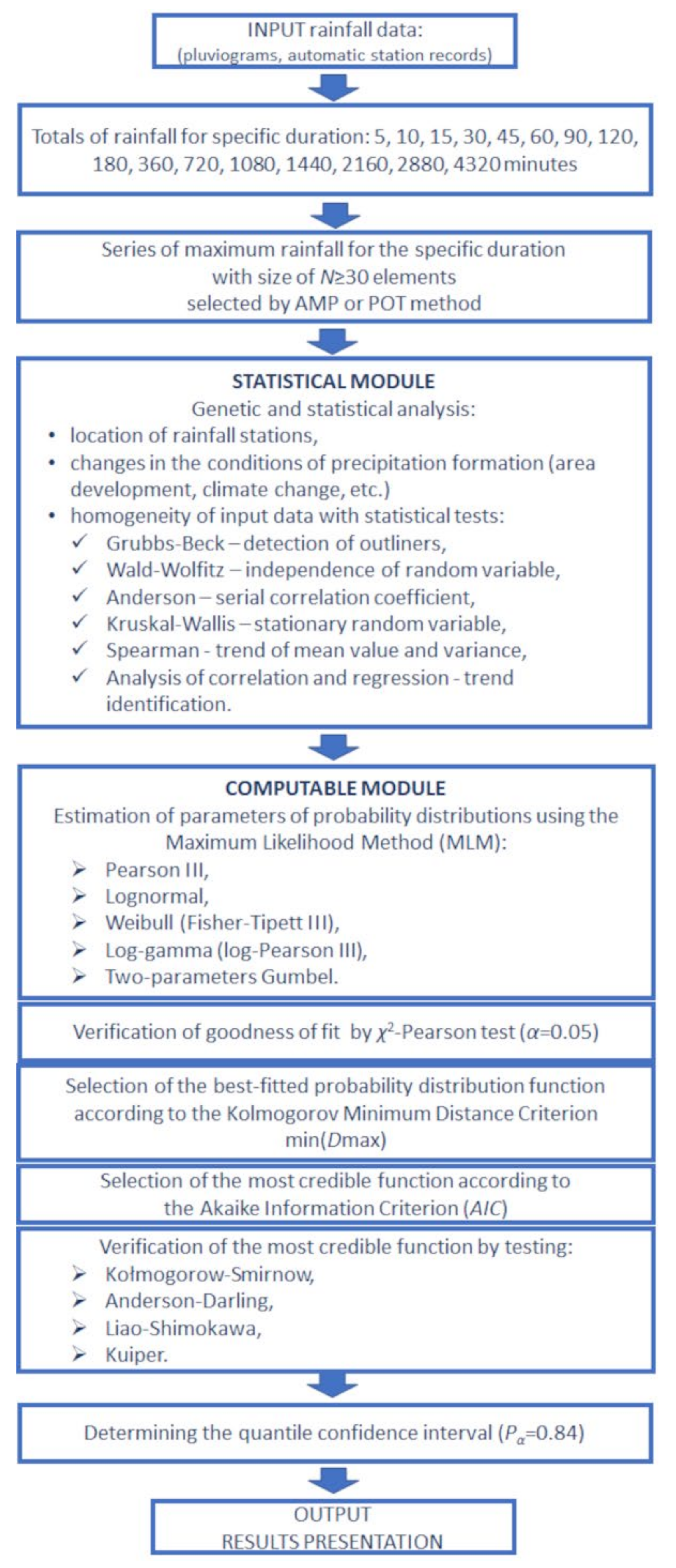
The PMAXTP model for a frequency analysis of maximum precipitation with a specified duration and probability of exceedance was developed with the use of the method of alternative events (MAE), which serves to compute annual maximum flows with a specified probability of exceedance [35]. The overall scheme of the PMAXTP model is shown in Figure 1. The model contains two computational modules, one that performs a statistical analysis of series of precipitation data, and another that estimates maximum precipitation with a given duration and probability of exceedance. The latter includes an estimation of parameters of the distributions by the maximum likelihood method, verification of goodness of fit by Pearson’s χ² test, selection of the best-fitting probability distribution function within each distribution type according to the criterion of minimum Kolmogorov distance, selection of the most credible function according to the Akaike information criterion (AIC), and determination of the quantile confidence interval with regard to the randomness of the series of observations. The results returned by the PMAXTP model are values of maximum precipitation with a specified duration τ (min) ∈ {5, 10, 15, 30, 45, 60, 90, 120, 180, 360, 720, 1080, 1440, 2160, 2880, 4320} and a given probability of exceedance p (%) ∈ {99.9, 99.5, 99, 98.5, 98, 95, 90, 80, 70, 60, 50, 40, 30, 20, 10, 5, 3, 2, 1, 0.5, 0.3, 0.2, 0.1, 0.05, 0.03, 0.02, 0.01}.

An analysis of the homogeneity of the random variables of series of maximum precipitation with different durations was performed by genetic (physical) methods and by statistical methods [35,36]. The identification of the trend of the analyzed random variables and evaluation of the form of the trend function were carried out by correlation and regression analysis, where the dependent variable is the maximum precipitation selected by the AMP or POT method, and the independent variable is the time (τ). The correlation was analyzed using the nonparametric Spearman rank correlation test [37] and the parametric Pearson linear correlation coefficient test [38]. In regression analysis, the global Fisher-Snedecor F-test [39] tests three equivalent null hypotheses: the significance of the slope, the significance of the coefficient of determination, and the significance of the linear relationship between the analyzed variables. Verification is performed for the null hypothesis that the independent variable (time τ) has no effect on the analyzed dependent variable, which here is the maximum precipitation $(P_{\tau }^{\mathrm{AMP}}$ and $P_{\tau }^{\mathrm{POT}})$. An evaluation of the form of the trend function is performed using scatter plots of the analyzed random variables with respect to time (τ). These provide a visual assessment and an evaluation of the form of the trend function: linear, power, exponential, etc.

The internal correlation of the analyzed random variable was checked using the Anderson autocorrelation coefficient test [40]. This analysis identifies the occurrence of periodic fluctuations and their effect on the variation of the analyzed variables. The results are presented numerically and graphically for a specified lag, with an indication of the autocorrelation coefficients and an evaluation of white noise (standard error) for the confidence level assumed (α).

The computation of the maximum precipitation with a specified probability of exceedance is performed using probabilistic models of the properties of the random variables $P_{\tau }^{\mathrm{AMP}}$ and $P_{\tau }^{\mathrm{POT}}$. An analysis of the properties of random maximum precipitations served as the basis for the acceptance of potential probability distribution models: e.g., G, GA, LN, log-gamma (LGA), and WE. The first four models are three-parameter distributions with the following parameters: α (α > 0), λ (λ > 0) or μ (μ > 0), and ε (ε ≤ x ≤ + ∞), representing, respectively, the parameters of scale, shape, and position, i.e., the lower (left-hand) limit of the probability distribution (see details in Appendix A).

The PMAXTP model assumes that each type of distribution is represented by a family of functions f_i(x), shifted with respect to each other, each of which has a certain fixed lower limit (ε_i) satisfying $0\le {\epsilon }_i<\underset{1\le j\le n}{\min }\left(x_j\right)$, where $n$ is the size of the random sample. The value of ε_i may take values ranging from 0 up to the minimum value of the variable (X) in the random sample $\left(x_1,x_2, \cdots , x_n\right)$. Hence, the lower limit (ε_i) of the ith specific function in the family of a selected type of distributions is the discriminant of that function within the family, and is not subject to estimation. In the G distribution, described by Equations (A9) and (A10) in Appendix A, only two parameters appear: the scale α and the shape μ.

The parameters of probability density functions were estimated by the MLM using dedicated software [41]. The procedure was as follows:

(i)

Estimation of parameters of four types of functions belonging to the probability distribution families GA, WE, LGA, and LN for a fixed value and range of variation of the distribution lower limit ε_i for the ith function belonging to the family of the selected probability distribution. In the case of the G distribution, the parameters are estimated for a single function; there is no distribution lower limit (ε).

(ii)

Obtainment of i sets of estimated values of parameters for each selected probability distribution function by the solution of systems of equations according to explicit formulas, or the determination of a set of parameter values using Brent’s or Newton’s numerical methods [42].

(iii)

Check of the goodness of fit of the selected theoretical distribution with the empirical distribution using Pearson’s χ² test [43] at a significance level α = 0.05.

(iv)

Formation of a set of noncontradictory probability distribution functions from all probability distribution functions for which the hypothesis of goodness of fit was not rejected. Sets of noncontradictory functions are formed separately for each selected probability distribution function type: GA, WE, LGA, and LN.

(v)

Selection of the best-fitting function within each distribution type. For each theoretical distribution type used, there may exist many noncontradictory functions with different lower limit values ε_i. A single function is selected for each distribution type (GA, WE, LGA, LN) according to the criterion of minimum Kolmogorov distance, min(D_max) [35,44]. The probability distribution function for which, within a given distribution type, the Kolmogorov distance D_max attains its minimum value is called the best-fitting function in the sense of the Kolmogorov distance criterion. These single functions, identified for each of the distribution types used, form the set of best-fitting functions.

(vi)

Selection of the most credible probability distribution function from the set of best-fitting functions of particular types (GA, WE, LGA, LN, G), performed by computing the value of the Akaike information criterion (AIC) [45] for each of those functions. The most credible function is taken to be the function with the smallest AIC value.

(vii)

Verification of the most credible distribution of maximum precipitation values, $P_{\tau }^{\mathrm{AMP}}$ and $P_{\tau }^{\mathrm{POT}}$, was based on nonparametric tests used to analyze the goodness-of-fit of a theoretical mathematical model to an empirical model. The verification of the distributions was concentrated on their tail part. The tails of the distributions are significant in terms of the occurrence of extreme values of the random variable, that is, values with a very low probability of exceedance. Thus, to evaluate the goodness-of-fit of the distributions, the following single-dimensional statistical tests were used: the Kolmogorov-Smirnov test (D_K-S) [46,47], the Anderson-Darling test (D_A-D) [48], the Liao-Shimokawa test (D_L-S) [49], and Kuiper’s test (D_K) [50]. (For details, see Appendix B.) The D_K-S test may be used for the verification of large deviations of a theoretical cumulative probability distribution from the empirical distribution. The D_A-D test is sensitive to deviations in the tail part, while the D_L-S test represents a weighted mean distance between the theoretical and empirical probability distributions in the whole range of the analyzed random variable, and is regarded as the most suitable for verification of the Gumbel and Weibull distributions [49]. The D_K test was used to verify the goodness-of-fit of the distribution in its central part, as well as in the lower and upper parts of the tail of the distribution.

(viii)

Selection of a probabilistic model, performed by comparing the estimated quantile errors resulting from the randomness of the sample of maximum precipitations with a specified duration τ selected by the AMP and POT methods $(P_{\tau }^{\mathrm{AMP}}$ and $P_{\tau }^{\mathrm{POT}})$.

3. Study Area and Data

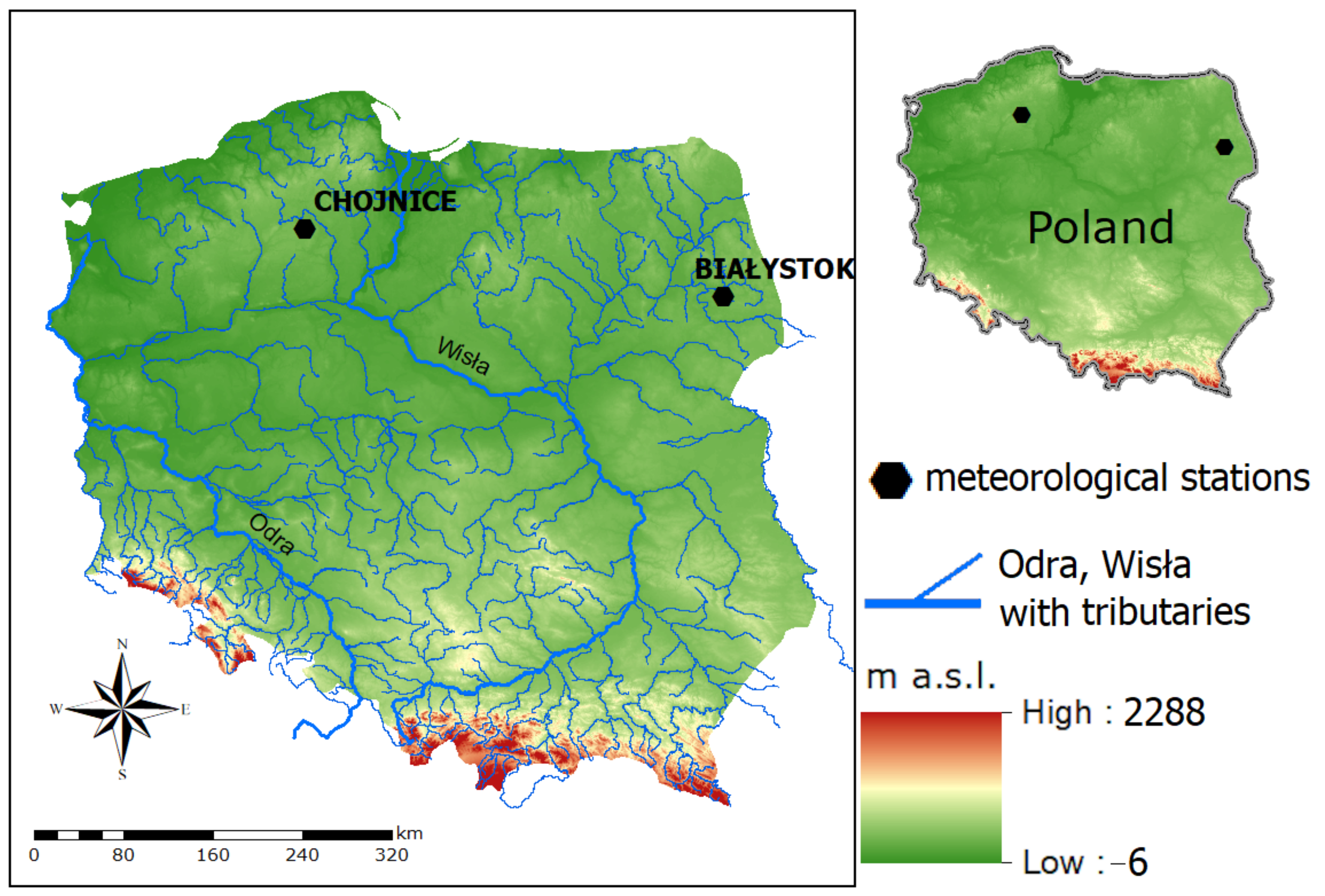
The PMAXTP model was tested on data from two meteorological stations located in Poland: Chojnice and Bialystok (Figure 2, black hexagons). The choice of stations was based on the availability of long series of historical data and current meteorological observations.

Data were drawn from the Rain-Brain database, created under the Development and Implementation of a Polish Atlas of Rainfall Intensities (PANDa) project [51] carried out in 2016 and 2017 by Poland’s Institute of Meteorology and Water Management—National Research Institute (IMGW—PIB). Under the PANDa project, a series of depths of precipitation having specific durations were subjected to qualitative assessment, including a comparison of digital records with analog data (from Hellmann rain gauges), and information was drawn from a system of ground-based radars operating in the measurement and observation network of the IMGW—PIB. The observations were verified with respect to the occurrence of meteorological configurations which might cause rainfall of a given quantity in specified pressure conditions, characteristic of the analyzed region.

The study was based on the 30 highest precipitation depth values for 16 specified durations, τ = {5, 10, 15, 30, 45, 60, 90, 120, 180, 360, 720, 1080, 1440, 2160, 2880, 4320} (minutes) for the two precipitation stations mentioned above.

Two methods were used to select maximum precipitation values: AMP [1,2,52] and POT [53]. Under the AMP method, a single maximum precipitation value was selected for the year, independent of its duration. A defect of the AMP method is that it fails to take into account all the high precipitation depth values occurring in a given year. In the POT method, it is possible to take into account all high precipitation depth values in a given year, i.e., the method selects these values that exceed a threshold determined a priori. The analyses were based on events with values not less than $P_{\min ,\tau }^{\mathrm{POT}}$ = 3.5τ^0.275 [51]. Thus, threshold values $P_{\tau }^{\mathrm{MAX}}$ (mm) were set for precipitation with specified durations (τ), as given in

Table 1. Minimum quantity of precipitation $P_{\min ,\tau }^{\mathrm{POT}}$ (mm) taken as a threshold in the POT method.

τ (min)	5	10	15	30	45	60	90	120	180	360	720	1080	1440	2160	2880	4320
$P_{\min ,\tau }^{\mathrm{POT}}$ (mm)	5.4	6.6	7.4	8.9	10.0	10.8	12.1	13.1	14.6	17.7	21.4	23.9	25.9	28.9	31.3	35.0

[51]. The subsequent analyses used 30-element series of maximum precipitation data, selected by both methods.

4. Results and Discussion

4.1. Results of Analysis of Homogeneity for the PMAXTP Model

An analysis was made of the genetic, time, and measurement homogeneity of the precipitation series from the stations in Chojnice and Bialystok. Based on a visual assessment of the measurement series and information contained in IMGW—PIB reports (Meteorological Yearbooks and Precipitation Yearbooks Report [51]), no significant factors were found that might have an impact on the genetic homogeneity of the series of maximum precipitation values observed in the years 1986–2015.

An analysis was made of the statistical properties of the series of precipitation measurements from Chojnice and Bialystok using nonparametric significance tests [35,36]. The results are presented in Table 2, Table 3, Table 4, Table 5 and Table 6. Table 2 and Table 3 contain the results of outlier detection using the Grubbs-Beck test [54,55], checking for the independence of the analyzed random variable using the Wald-Wolfowitz test (Test of Series) and Anderson serial autocorrelation coefficient test [40,55,56], and checking the stationarity of the analyzed random variable using the Kruskal-Wallis test and Spearman rank correlation coefficient test for the trends of mean and variance [57,58]. The final column of Table 2 and Table 3 indicates genetically and statistically homogeneous series of maximum precipitation data selected by the AMP and POT methods.

In the case of $P_{\tau }^{\mathrm{AMP}},$ the Grubbs-Beck test detected outliers for precipitation with the duration τ = 360 and τ = 720 min, at both the Chojnice station (Table 2) and the Bialystok station (Table 3). In Table 2 and Table 3, for a positive test result (+), the number of the outlier in the chronological sequence and the quantity of precipitation are also given. For the $P_{\tau }^{\mathrm{POT}}$ series at Chojnice (Table 2), outliers were detected for τ $\in$ {15, 30} and τ $\in$ {120, …, 4320} min, while at Bialystok (Table 3), outliers were detected for τ $\in$ {5, …, 15}, τ $\in$ {60, …, 360} and τ $\in$ {2160, …, 4320} min. Based on the theorem developed by Neyman and Scott [59] stating that the families of LN, G, and WE distributions—these being the distributions assumed as potential models describing the maximum precipitation values—are entirely susceptible to the occurrence of outliers in a random sample, it was concluded that the occurrence of the detected outliers should be considered entirely natural, and such elements were not removed from the measurement series.

Table 2. Results of nonhomogeneity analysis of AMP and POT precipitation series from Chojnice meteorological station; (−)/(+) denotes, respectively, negative and positive test results; √—denotes homogenous series.

τ (min)	Grubbs-Beck Test ±Outliers (mm)		Test of Series		Kruskal-Wallis Test		Spearman Rank Correlation Test				Homogeneity of Precipitation $P_{\tau }^{\mathrm{MAX}}$
							for Trend of Mean		for Trend of Variance
	AMP	POT	AMP	POT	AMP	POT	AMP	POT	AMP	POT	AMP	POT
5	(−)	(−)	(−)	(−)	(−)	(−)	(−)	(−)	(−)	(−)	√	√
10	(−)	(−)	(−)	(−)	(−)	(−)	(−)	(−)	(−)	(−)
15	(−)	(+) [5] = 24.5	(−)	(−)	(+)	(−)	(+)	(−)	(+)	(−)		√
30	(−)	(+) [4] = 33.7	(−)	(−)	(+)	(−)	(+)	(−)	(+)	(−)		√
45	(−)	(−)	(−)	(−)	(+)	(−)	(+)	(−)	(+)	(+)
60	(−)	(−)	(−)	(−)	(+)	(−)	(+)	(−)	(−)	(+)
90	(−)	(−)	(−)	(−)	(+)	(−)	(+)	(−)	(−)	(−)		√
120	(−)	(+) [19] = 42.9	(−)	(−)	(+)	(−)	(+)	(−)	(−)	(−)		√
180	(−)	(+) [19] = 48.4	(−)	(−)	(+)	(−)	(+)	(−)	(+)	(−)		√
360	(+) [25] = 60.3	(+) [24] = 60.3	(−)	(−)	(+)	(−)	(+)	(−)	(+)	(−)		√
720	(+) [4] = 11.8 [25] = 67.7	(+) [24] = 67.6	(−)	(−)	(−)	(−)	(−)	(−)	(−)	(−)	√	√
1080	(+) [4] = 11.8	(+) [24] = 71.9	(−)	(−)	(−)	(−)	(−)	(−)	(−)	(−)	√	√
1440	(−)	(+) [25] = 71.9	(−)	(−)	(−)	(−)	(−)	(−)	(−)	(−)	√	√
2160	(−)	(+) [20] = 80.5	(−)	(−)	(−)	(−)	(−)	(−)	(−)	(−)	√	√
2880	(−)	(+) [22] = 87.2	(−)	(−)	(−)	(−)	(−)	(−)	(−)	(−)	√	√
4320	(−)	(+) [21] = 87.9	(−)	(−)	(−)	(−)	(−)	(−)	(−)	(−)	√	√

Table 2. Results of nonhomogeneity analysis of AMP and POT precipitation series from Chojnice meteorological station; (−)/(+) denotes, respectively, negative and positive test results; √—denotes homogenous series.

τ (min)	Grubbs-Beck Test ±Outliers (mm)		Test of Series		Kruskal-Wallis Test		Spearman Rank Correlation Test				Homogeneity of Precipitation $P_{\tau }^{\mathrm{MAX}}$
							for Trend of Mean		for Trend of Variance
	AMP	POT	AMP	POT	AMP	POT	AMP	POT	AMP	POT	AMP	POT
5	(−)	(−)	(−)	(−)	(−)	(−)	(−)	(−)	(−)	(−)	√	√
10	(−)	(−)	(−)	(−)	(−)	(−)	(−)	(−)	(−)	(−)
15	(−)	(+) [5] = 24.5	(−)	(−)	(+)	(−)	(+)	(−)	(+)	(−)		√
30	(−)	(+) [4] = 33.7	(−)	(−)	(+)	(−)	(+)	(−)	(+)	(−)		√
45	(−)	(−)	(−)	(−)	(+)	(−)	(+)	(−)	(+)	(+)
60	(−)	(−)	(−)	(−)	(+)	(−)	(+)	(−)	(−)	(+)
90	(−)	(−)	(−)	(−)	(+)	(−)	(+)	(−)	(−)	(−)		√
120	(−)	(+) [19] = 42.9	(−)	(−)	(+)	(−)	(+)	(−)	(−)	(−)		√
180	(−)	(+) [19] = 48.4	(−)	(−)	(+)	(−)	(+)	(−)	(+)	(−)		√
360	(+) [25] = 60.3	(+) [24] = 60.3	(−)	(−)	(+)	(−)	(+)	(−)	(+)	(−)		√
720	(+) [4] = 11.8 [25] = 67.7	(+) [24] = 67.6	(−)	(−)	(−)	(−)	(−)	(−)	(−)	(−)	√	√
1080	(+) [4] = 11.8	(+) [24] = 71.9	(−)	(−)	(−)	(−)	(−)	(−)	(−)	(−)	√	√
1440	(−)	(+) [25] = 71.9	(−)	(−)	(−)	(−)	(−)	(−)	(−)	(−)	√	√
2160	(−)	(+) [20] = 80.5	(−)	(−)	(−)	(−)	(−)	(−)	(−)	(−)	√	√
2880	(−)	(+) [22] = 87.2	(−)	(−)	(−)	(−)	(−)	(−)	(−)	(−)	√	√
4320	(−)	(+) [21] = 87.9	(−)	(−)	(−)	(−)	(−)	(−)	(−)	(−)	√	√

Table 3. Results of nonhomogeneity analysis of AMP and POT precipitation series from Bialystok meteorological station; (−)/(+) denotes, respectively, negative and positive test results; √—denotes homogenous series.

τ (min)	Grubbs-Beck Test ±Outliers (mm)		Test of Series		Kruskal-Wallis Test		Spearman Rank Correlation Test				Homogeneity of Precipitation $P_{\tau }^{\mathrm{MAX}}$
							for Trend of Mean		for Trend of Variance
	AMP	POT	AMP	POT	AMP	POT	AMP	POT	AMP	POT	AMP	POT
5	(−)	(+) [15] = 15.5	(−)	(−)	(+)	(−)	(+)	(−)	(−)	(−)		√
10	(−)	(+) [15] = 22.3	(−)	(−)	(+)	(−)	(+)	(−)	(−)	(−)		√
15	(−)	(+) [17] = 24.6	(−)	(−)	(+)	(+)	(+)	(−)	(−)	(+)
30	(−)	(−)	(−)	(−)	(+)	(+)	(+)	(−)	(−)	(+)
45	(−)	(−)	(−)	(−)	(+)	(−)	(+)	(−)	(−)	(−)		√
60	(−)	(−)	(−)	(−)	(+)	(−)	(+)	(−)	(−)	(−)		√
90	(−)	(+) [22] = 42.0	(−)	(−)	(+)	(−)	(+)	(−)	(−)	(−)		√
120	(−)	(+) [23] = 47.7	(−)	(−)	(+)	(−)	(+)	(−)	(−)	(+)
180	(−)	(+) [23] = 52.2	(−)	(−)	(+)	(−)	(+)	(−)	(−)	(−)		√
360	(+) [4] = 10.89 [25] = 67.70	(+) [23] = 67.7	(−)	(−)	(+)	(+)	(+)	(+)	(−)	(−)
720	(+) [25] = 73.90	(+) [21] = 73.9	(−)	(−)	(+)	(−)	(+)	(−)	(−)	(−)		√
1080	(−)	(+) [20] = 79.6	(−)	(−)	(+)	(−)	(+)	(−)	(−)	(−)		√
1440	(−)	(+) [23] = 84.50	(−)	(−)	(+)	(+)	(+)	(+)	(−)	(−)
2160	(−)	(+) [21] = 101.30	(−)	(−)	(+)	(−)	(+)	(−)	(−)	(−)		√
2880	(−)	(+) [20] = 106.20	(−)	(−)	(+)	(−)	(+)	(−)	(−)	(−)		√
4320	(−)	(−)	(−)	(−)	(+)	(−)	(+)	(−)	(−)	(−)		√

Table 3. Results of nonhomogeneity analysis of AMP and POT precipitation series from Bialystok meteorological station; (−)/(+) denotes, respectively, negative and positive test results; √—denotes homogenous series.

τ (min)	Grubbs-Beck Test ±Outliers (mm)		Test of Series		Kruskal-Wallis Test		Spearman Rank Correlation Test				Homogeneity of Precipitation $P_{\tau }^{\mathrm{MAX}}$
							for Trend of Mean		for Trend of Variance
	AMP	POT	AMP	POT	AMP	POT	AMP	POT	AMP	POT	AMP	POT
5	(−)	(+) [15] = 15.5	(−)	(−)	(+)	(−)	(+)	(−)	(−)	(−)		√
10	(−)	(+) [15] = 22.3	(−)	(−)	(+)	(−)	(+)	(−)	(−)	(−)		√
15	(−)	(+) [17] = 24.6	(−)	(−)	(+)	(+)	(+)	(−)	(−)	(+)
30	(−)	(−)	(−)	(−)	(+)	(+)	(+)	(−)	(−)	(+)
45	(−)	(−)	(−)	(−)	(+)	(−)	(+)	(−)	(−)	(−)		√
60	(−)	(−)	(−)	(−)	(+)	(−)	(+)	(−)	(−)	(−)		√
90	(−)	(+) [22] = 42.0	(−)	(−)	(+)	(−)	(+)	(−)	(−)	(−)		√
120	(−)	(+) [23] = 47.7	(−)	(−)	(+)	(−)	(+)	(−)	(−)	(+)
180	(−)	(+) [23] = 52.2	(−)	(−)	(+)	(−)	(+)	(−)	(−)	(−)		√
360	(+) [4] = 10.89 [25] = 67.70	(+) [23] = 67.7	(−)	(−)	(+)	(+)	(+)	(+)	(−)	(−)
720	(+) [25] = 73.90	(+) [21] = 73.9	(−)	(−)	(+)	(−)	(+)	(−)	(−)	(−)		√
1080	(−)	(+) [20] = 79.6	(−)	(−)	(+)	(−)	(+)	(−)	(−)	(−)		√
1440	(−)	(+) [23] = 84.50	(−)	(−)	(+)	(+)	(+)	(+)	(−)	(−)
2160	(−)	(+) [21] = 101.30	(−)	(−)	(+)	(−)	(+)	(−)	(−)	(−)		√
2880	(−)	(+) [20] = 106.20	(−)	(−)	(+)	(−)	(+)	(−)	(−)	(−)		√
4320	(−)	(−)	(−)	(−)	(+)	(−)	(+)	(−)	(−)	(−)		√

For all observed values of maximum precipitation $P_{\tau }^{\mathrm{AMP}}$ and $P_{\tau }^{\mathrm{POT}}$ (Table 2 and Table 3), the Wald-Wolfowitz test (Test of Series) and the Anderson serial correlation coefficient test showed that the analyzed measurement series were random and formed a simple sample, i.e., the random variables were independent variables. The significance level α = 0.05 used in the test took account of the size of the random sample, n = 30. For series of length greater than 30, a lower value may be taken as the test significance level (e.g., α = 0.01). For the detection of outliers with the Grubbs-Beck test, the higher value α = 0.10 was used, on the assumption that series of measurements of meteorological phenomena may be characterized by greater anthropogenic impact.

The stationarity of the measurement series was checked using the Kruskal-Wallis test and Spearman rank correlation test for the trends of the mean and variance. According to the Kruskal-Wallis test, in the $P_{\tau }^{\mathrm{AMP}}$ series from both Chojnice and Bialystok, jumps in the mean were detected, with the exception of the observations for τ = 5 and τ $\in$ {720, …, 4320} min at Chojnice. In the case of the $P_{\tau }^{\mathrm{POT}}$ precipitation values, most of the observations were stationary, with the exception of τ = 5 at Chojnice and τ $\in$ {15, 30} and τ = 1440 min at Bialystok.

The Spearman’s rank correlation test for the trends of mean and variance revealed nonstationarity mainly for the $P_{\tau }^{\mathrm{AMP}}$ precipitation values. In the case of $P_{\tau }^{\mathrm{POT}}$, nonstationary observations were the exception. For example, in the observations from Chojnice for τ = 10 min and τ $\in$ {45, 60} min, a trend was detected in the mean and variance, respectively, while for the Bialystok data, such trends were detected, respectively, for τ $\in$ {360, 1440} and τ = 120 min.

The results of correlation testing and the identification of the trend of maximum precipitation for the AMP and POT series are given in Table 4, Table 5 and Table 6. The identification of the trend of the analyzed random variables was performed using the nonparametric Spearman rank correlation test [37] and the parametric Pearson linear correlation coefficient test [38]. An analysis was made of the correlation between the studied random variables ($P_{\mathsf{\tau }}^{\mathrm{AMP}}$ and $P_{\mathsf{\tau }}^{\mathrm{POT}}$) and the time variable τ (Table 4). Positive and negative values indicate upward and downward trends, respectively. Spearman’s coefficient also indicates the strength of the trend. The closer the values are to 1.0, the stronger is the relationship between the analyzed random variable and the time variable τ. Pearson’s coefficient indicates proportionality, that is, linear dependence between variables, while Spearman’s coefficient indicates any monotonic relationship, even if nonlinear. Figures shown in bold type in Table 4 indicate significant correlations, with the probability p ≤ 0.05. Strong dependences between the observed maximum precipitation values and the independent variable τ were recorded in the case of $P_{\mathsf{\tau }}^{\mathrm{AMP}}$ at both Chojnice and Bialystok.

Table 4. Correlations between the maximum precipitation variables and time τ for the Chojnice and Bialystok stations. Bold values of Spearman’s rank correlation and Pearson’s linear correlation coefficients are significant at p < 0.05 for n = 30, where n is the size of the sample.

τ (min)	5	10	15	30	45	60	90	120	180	360	720	1080	1440	2160	2880	4320
Nonparametric Spearman rank correlation coefficient test for CHOJNICE station
$P_{\tau }^{\mathrm{AMP}}$	0.277	0.309	0.396	0.481	0.452	0.472	0.439	0.495	0.516	0.458	0.198	0.100	0.136	0.112	0.206	0.220
$P_{\tau }^{\mathrm{POT}}$	0.175	−0.449	−0.181	−0.270	−0.019	−0.169	−0.129	−0.046	−0.319	0.036	−0.201	−0.203	−0.226	−0.326	−0.285	−0.340
Parametric Pearson linear correlation coefficient test for CHOJNICE station
$P_{\tau }^{\mathrm{AMP}}$	0.267	0.297	0.290	0.292	0.303	0.335	0.388	0.434	0.425	0.387	0.299	0.186	0.159	0.101	0.189	0.210
$P_{\tau }^{\mathrm{POT}}$	0.209	−0.299	−0.255	−0.331	−0.124	−0.235	−0.142	−0.068	−0.222	0.090	0.046	−0.045	−0.114	−0.205	−0.145	−0.193
Nonparametric Spearman rank correlation coefficient test for BIAŁYSTOK station
$P_{\tau }^{\mathrm{AMP}}$	0.584	0.552	0.553	0.524	0.471	0.477	0.482	0.458	0.482	0.454	0.470	0.415	0.458	0.433	0.417	0.366
$P_{\tau }^{\mathrm{POT}}$	0.181	0.007	0.222	0.227	0.042	0.056	0.137	0.271	0.194	0.434	0.315	0.236	0.407	0.251	0.067	0.353
Parametric Pearson linear correlation coefficient test for BIAŁYSTOK station
$P_{\tau }^{\mathrm{AMP}}$	0.448	0.490	0.489	0.427	0.399	0.396	0.428	0.411	0.466	0.468	0.486	0.457	0.456	0.451	0.434	0.423
$P_{\tau }^{\mathrm{POT}}$	0.131	0.054	0.174	0.115	0.018	0.006	0.102	0.168	0.195	0.375	0.368	0.304	0.371	0.228	0.129	0.364

Table 4. Correlations between the maximum precipitation variables and time τ for the Chojnice and Bialystok stations. Bold values of Spearman’s rank correlation and Pearson’s linear correlation coefficients are significant at p < 0.05 for n = 30, where n is the size of the sample.

τ (min)	5	10	15	30	45	60	90	120	180	360	720	1080	1440	2160	2880	4320
Nonparametric Spearman rank correlation coefficient test for CHOJNICE station
$P_{\tau }^{\mathrm{AMP}}$	0.277	0.309	0.396	0.481	0.452	0.472	0.439	0.495	0.516	0.458	0.198	0.100	0.136	0.112	0.206	0.220
$P_{\tau }^{\mathrm{POT}}$	0.175	−0.449	−0.181	−0.270	−0.019	−0.169	−0.129	−0.046	−0.319	0.036	−0.201	−0.203	−0.226	−0.326	−0.285	−0.340
Parametric Pearson linear correlation coefficient test for CHOJNICE station
$P_{\tau }^{\mathrm{AMP}}$	0.267	0.297	0.290	0.292	0.303	0.335	0.388	0.434	0.425	0.387	0.299	0.186	0.159	0.101	0.189	0.210
$P_{\tau }^{\mathrm{POT}}$	0.209	−0.299	−0.255	−0.331	−0.124	−0.235	−0.142	−0.068	−0.222	0.090	0.046	−0.045	−0.114	−0.205	−0.145	−0.193
Nonparametric Spearman rank correlation coefficient test for BIAŁYSTOK station
$P_{\tau }^{\mathrm{AMP}}$	0.584	0.552	0.553	0.524	0.471	0.477	0.482	0.458	0.482	0.454	0.470	0.415	0.458	0.433	0.417	0.366
$P_{\tau }^{\mathrm{POT}}$	0.181	0.007	0.222	0.227	0.042	0.056	0.137	0.271	0.194	0.434	0.315	0.236	0.407	0.251	0.067	0.353
Parametric Pearson linear correlation coefficient test for BIAŁYSTOK station
$P_{\tau }^{\mathrm{AMP}}$	0.448	0.490	0.489	0.427	0.399	0.396	0.428	0.411	0.466	0.468	0.486	0.457	0.456	0.451	0.434	0.423
$P_{\tau }^{\mathrm{POT}}$	0.131	0.054	0.174	0.115	0.018	0.006	0.102	0.168	0.195	0.375	0.368	0.304	0.371	0.228	0.129	0.364

The form of the trend function was assessed using regression analysis (Table 5 and Table 6), where the dependent variable is the maximum precipitation and the independent variable is the time τ. Table 5 and Table 6 give the results of the regression analysis, including the following indicators: Pearson’s correlation coefficient r, the coefficient of determination r², the Fisher-Snedecor global F-test [60], the test probability p resulting from the latter test, the size of the random sample n, and the standard error of estimation S(E). Statistically significant regression coefficients for the analyzed variables are identified according to the criterion for statistical significance adopted in the model, with α = 0.05. This means that the regression coefficients are significant for a test probability p ≤ 0.05.

The global F-test tests three equivalent null hypotheses: H₀: β₁ = 0 (significance of the slope); H₀: r² = 0 (significance of the coefficient of determination); and H₀: y = β₁x+ β₀ (significance of the linear relationship between the analyzed variables), where β₁ is the slope; β₀ is a free term; and x and y denote the independent and dependent variables, respectively. Verification is made of the null hypothesis that the independent variable x (in Table 5 and Table 6, the independent variable is time, τ) does not influence the analyzed dependent variable y (in Table 5 and Table 6, the dependent variables are $P_5^{\mathrm{AMP}}$, …, $P_{4320}^{\mathrm{AMP}}$ and $P_5^{\mathrm{POT}}$, …, $P_{4320}^{\mathrm{POT}}$). If, in the course of verification, the null hypothesis is rejected, the regression coefficient is assessed as significant, meaning that τ has a significant influence on the analyzed dependent variable. Examples of random variables with no trend and showing a trend are given in Table 5 and Table 6, respectively, for observations from Chojnice and Bialystok.

Table 5. Results of simple regression analysis for the Chojnice station, where the dependent variables are $P_{\tau }^{\mathrm{AMP}}$ and $P_{\tau }^{\mathrm{POT}}$, and the independent variable is time (τ), for n = 30, where r is Pearson’s correlation coefficient; r² is the coefficient of determination; F(1,n) is the Fisher-Snedecor test; S(E) is the standard error of estimation; and p (p-value) is the value of the test probability. Bold type indicates significance of regression parameters, namely the existence (for p ≤ 0.05) of a significant linear trend coefficient.

τ	$P_{\tau }^{\mathrm{AMP}}$—CHOJNICE					$P_{\tau }^{\mathrm{POT}}$—CHOJNICE
	r	r2	F(1,n = 28)	S(E)	p	r	r2	F(1,n = 28)	S(E)	p
5	0.266	0.071	2.142	2.278	0.154	0.208	0.043	1.274	1.374	0.268
10	0.297	0.088	2.718	3.780	0.110	0.299	0.089	2.751	2.641	0.108
15	0.296	0.087	2.691	4.872	0.112	0.255	0.065	1.949	3.754	0.173
30	0.292	0.085	2.609	6.916	0.117	0.331	0.109	3.447	5.396	0.073
45	0.302	0.092	2.824	7.244	0.103	0.124	0.015	0.440	5.757	0.512
60	0.335	0.112	3.545	7.244	0.070	0.234	0.055	1.634	5.596	0.211
90	0.388	0.151	4.967	7.399	0.034	0.142	0.020	0.577	5.762	0.453
120	0.434	0.188	6.513	7.623	0.016	0.067	0.004	0.128	5.983	0.722
180	0.425	0.181	6.181	8.089	0.019	0.221	0.049	1.447	6.489	0.238
360	0.386	0.149	4.926	9.047	0.034	0.090	0.008	0.229	7.484	0.635
720	0.298	0.089	2.744	9.857	0.108	0.046	0.002	0.059	7.524	0.808
1080	0.185	0.034	0.998	12.241	0.326	0.045	0.002	0.056	9.465	0.813
1440	0.158	0.025	0.726	13.263	0.401	0.113	0.012	0.366	10.337	0.550
2160	0.101	0.010	0.289	15.139	0.594	0.204	0.042	1.226	11.338	0.277
2880	0.188	0.035	1.035	15.589	0.317	0.145	0.021	0.604	11.986	0.443
4320	0.209	0.043	1.287	16.387	0.266	0.193	0.037	1.086	12.190	0.306

Table 5. Results of simple regression analysis for the Chojnice station, where the dependent variables are $P_{\tau }^{\mathrm{AMP}}$ and $P_{\tau }^{\mathrm{POT}}$, and the independent variable is time (τ), for n = 30, where r is Pearson’s correlation coefficient; r² is the coefficient of determination; F(1,n) is the Fisher-Snedecor test; S(E) is the standard error of estimation; and p (p-value) is the value of the test probability. Bold type indicates significance of regression parameters, namely the existence (for p ≤ 0.05) of a significant linear trend coefficient.

τ	$P_{\tau }^{\mathrm{AMP}}$—CHOJNICE					$P_{\tau }^{\mathrm{POT}}$—CHOJNICE
	r	r2	F(1,n = 28)	S(E)	p	r	r2	F(1,n = 28)	S(E)	p
5	0.266	0.071	2.142	2.278	0.154	0.208	0.043	1.274	1.374	0.268
10	0.297	0.088	2.718	3.780	0.110	0.299	0.089	2.751	2.641	0.108
15	0.296	0.087	2.691	4.872	0.112	0.255	0.065	1.949	3.754	0.173
30	0.292	0.085	2.609	6.916	0.117	0.331	0.109	3.447	5.396	0.073
45	0.302	0.092	2.824	7.244	0.103	0.124	0.015	0.440	5.757	0.512
60	0.335	0.112	3.545	7.244	0.070	0.234	0.055	1.634	5.596	0.211
90	0.388	0.151	4.967	7.399	0.034	0.142	0.020	0.577	5.762	0.453
120	0.434	0.188	6.513	7.623	0.016	0.067	0.004	0.128	5.983	0.722
180	0.425	0.181	6.181	8.089	0.019	0.221	0.049	1.447	6.489	0.238
360	0.386	0.149	4.926	9.047	0.034	0.090	0.008	0.229	7.484	0.635
720	0.298	0.089	2.744	9.857	0.108	0.046	0.002	0.059	7.524	0.808
1080	0.185	0.034	0.998	12.241	0.326	0.045	0.002	0.056	9.465	0.813
1440	0.158	0.025	0.726	13.263	0.401	0.113	0.012	0.366	10.337	0.550
2160	0.101	0.010	0.289	15.139	0.594	0.204	0.042	1.226	11.338	0.277
2880	0.188	0.035	1.035	15.589	0.317	0.145	0.021	0.604	11.986	0.443
4320	0.209	0.043	1.287	16.387	0.266	0.193	0.037	1.086	12.190	0.306

Table 6. Results of simple regression analysis for the Bialystok station, where the dependent variables are $P_{\tau }^{\mathrm{AMP}}$ and $P_{\tau }^{\mathrm{POT}}$, and the independent variable is time (τ), for n = 30, where r is Pearson’s correlation coefficient; r² is the coefficient of determination; F(1,n) is the Fisher-Snedecor test; S(E) is the standard error of estimation; and p (p-value) is the value of the test probability. Bold type indicates significance of regression parameters, namely the existence (for p ≤ 0.05) of a significant influence of the variable τ on the analyzed dependent variable.

τ	$P_{\tau }^{\mathrm{AMP}}$—BIALYSTOK					$P_{\tau }^{\mathrm{POT}}$—BIALYSTOK
	r	r2	F(1,n = 28)	S(E)	p	r	r2	F(1,n = 28)	S(E)	p
5	0.489	0.240	8.846	2.407	0.006	0.253	0.064	1.915	1.840	0.177
10	0.4901	0.240	8.879	3.352	0.006	0.083	0.007	0.197	2.979	0.660
15	0.489	0.239	8.826	4.147	0.006	0.197	0.039	1.137	3.454	0.295
30	0.425	0.181	6.232	5.768	0.019	0.061	0.004	0.104	4.854	0.749
45	0.399	0.159	5.309	6.816	0.028	0.106	0.011	0.323	5.407	0.574
60	0.397	0.157	5.248	6.825	0.029	−0.017	0.0003	0.008	5.124	0.928
90	0.427	0.183	6.269	7.513	0.018	0.113	0.012	0.363	5.866	0.551
120	0.409	0.167	5.628	8.285	0.024	0.142	0.020	0.576	6.456	0.454
180	0.465	0.216	7.729	8.195	0.009	0.145	0.021	0.605	6.837	0.443
360	0.466	0.217	7.773	9.875	0.009	0.301	0.091	2.801	8.684	0.105
720	0.487	0.237	8.708	10.828	0.006	0.368	0.135	4.390	10.032	0.045
1080	0.459	0.212	7.513	12.186	0.010	0.376	0.142	4.624	11.615	0.040
1440	0.458	0.210	7.465	13.717	0.011	0.367	0.134	4.350	12.633	0.046
2160	0.454	0.206	7.267	16.796	0.012	0.287	0.083	2.531	15.312	0.123
2880	0.436	0.191	6.600	18.190	0.016	0.193	0.037	1.088	16.566	0.306
4320	0.426	0.182	6.217	21.715	0.018	0.359	0.129	4.152	19.319	0.515

Table 6. Results of simple regression analysis for the Bialystok station, where the dependent variables are $P_{\tau }^{\mathrm{AMP}}$ and $P_{\tau }^{\mathrm{POT}}$, and the independent variable is time (τ), for n = 30, where r is Pearson’s correlation coefficient; r² is the coefficient of determination; F(1,n) is the Fisher-Snedecor test; S(E) is the standard error of estimation; and p (p-value) is the value of the test probability. Bold type indicates significance of regression parameters, namely the existence (for p ≤ 0.05) of a significant influence of the variable τ on the analyzed dependent variable.

τ	$P_{\tau }^{\mathrm{AMP}}$—BIALYSTOK					$P_{\tau }^{\mathrm{POT}}$—BIALYSTOK
	r	r2	F(1,n = 28)	S(E)	p	r	r2	F(1,n = 28)	S(E)	p
5	0.489	0.240	8.846	2.407	0.006	0.253	0.064	1.915	1.840	0.177
10	0.4901	0.240	8.879	3.352	0.006	0.083	0.007	0.197	2.979	0.660
15	0.489	0.239	8.826	4.147	0.006	0.197	0.039	1.137	3.454	0.295
30	0.425	0.181	6.232	5.768	0.019	0.061	0.004	0.104	4.854	0.749
45	0.399	0.159	5.309	6.816	0.028	0.106	0.011	0.323	5.407	0.574
60	0.397	0.157	5.248	6.825	0.029	−0.017	0.0003	0.008	5.124	0.928
90	0.427	0.183	6.269	7.513	0.018	0.113	0.012	0.363	5.866	0.551
120	0.409	0.167	5.628	8.285	0.024	0.142	0.020	0.576	6.456	0.454
180	0.465	0.216	7.729	8.195	0.009	0.145	0.021	0.605	6.837	0.443
360	0.466	0.217	7.773	9.875	0.009	0.301	0.091	2.801	8.684	0.105
720	0.487	0.237	8.708	10.828	0.006	0.368	0.135	4.390	10.032	0.045
1080	0.459	0.212	7.513	12.186	0.010	0.376	0.142	4.624	11.615	0.040
1440	0.458	0.210	7.465	13.717	0.011	0.367	0.134	4.350	12.633	0.046
2160	0.454	0.206	7.267	16.796	0.012	0.287	0.083	2.531	15.312	0.123
2880	0.436	0.191	6.600	18.190	0.016	0.193	0.037	1.088	16.566	0.306
4320	0.426	0.182	6.217	21.715	0.018	0.359	0.129	4.152	19.319	0.515

Values shown in bold type in Table 5 and Table 6 indicate the presence of a significant influence of time τ on the analyzed random variable. In these cases, the estimated regression slope coefficients β₁ are significantly different from zero. At Chojnice, the observations of maximum precipitation showed a trend only in the case of $P_{\mathsf{\tau }}^{\mathrm{AMP}}$ for the durations τ $\in$ {90, …, 360} min. At Bialystok, however, in all of the analyzed observations of maximum precipitation $P_{\mathsf{\tau }}^{\mathrm{AMP}}$ and in three cases of $P_{\mathsf{\tau }}^{\mathrm{POT}}$ (τ $\in$ {720, …, 1440} min), an upward trend was detected. The test probability p determined for the computed regression coefficients was below the assumed significance level α = 0.05.

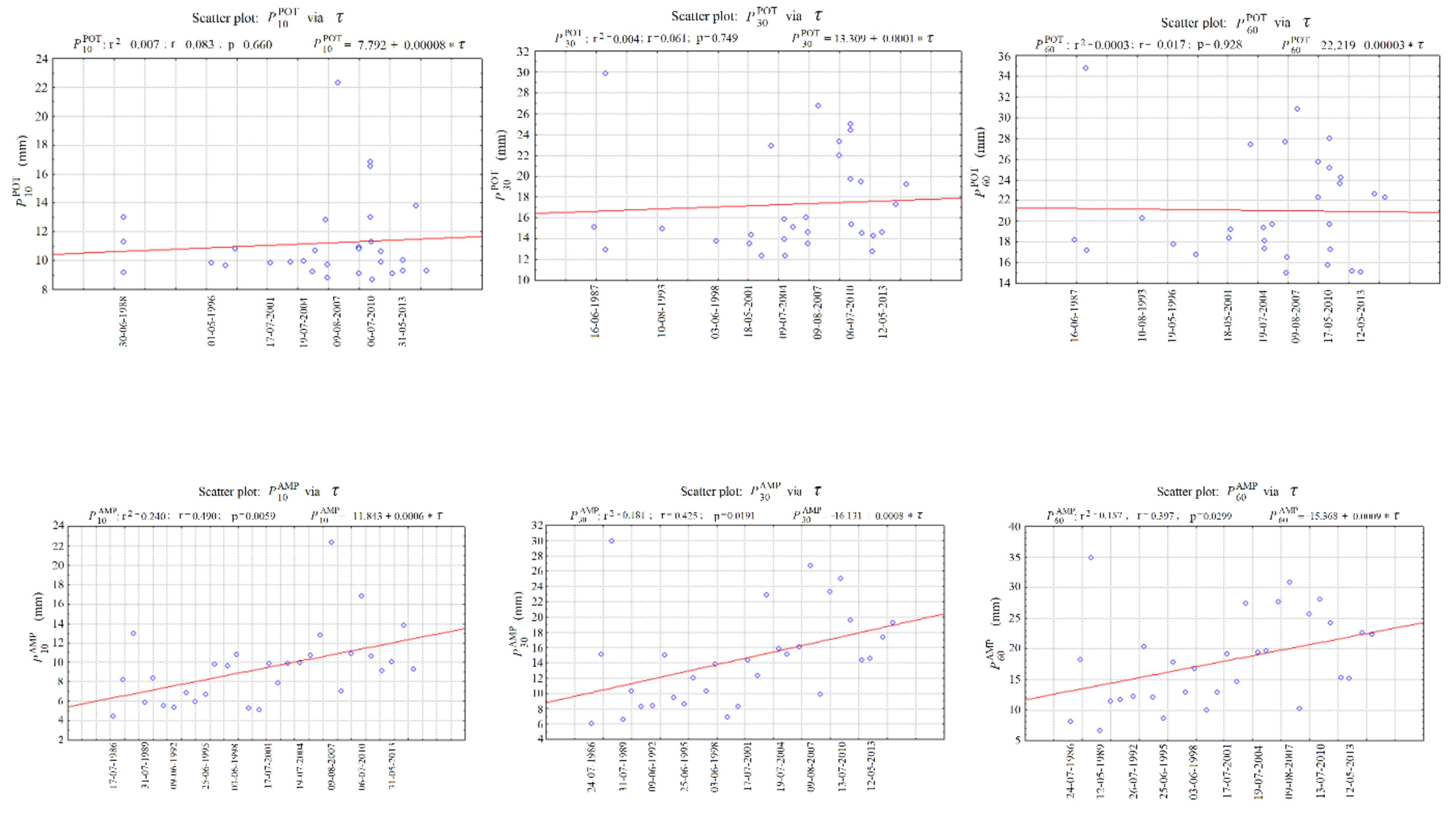
An assessment of the form of the trend function (linear, power, exponential, etc.) was made using scatter plots of the analyzed random variables with respect to time τ (Figure 3). The scatter plots of $P_{10}^{\mathrm{AMP}}$, $P_{30}^{\mathrm{AMP}},$ and $P_{60}^{\mathrm{AMO}}$ showed a clear linear upward trend, while those for the variables $P_{10}^{\mathrm{POT}}$, $P_{30}^{\mathrm{POT}},$ and $P_{60}^{\mathrm{POT}}$ showed, respectively, small upward and downward trends. In this case, the slope β₁ was close to 0, and the test probabilities ($P_{10}^{\mathrm{POT}}$: p = 0.660; $P_{30}^{\mathrm{POT}}$: p = 0.749; $P_{60}^{\mathrm{POT}}$: p = 0.928) were substantially higher than the significance level α = 0.05 used in the analysis. In the annual data, seasonal (monthly or daily) fluctuations were not analyzed. If the analyzed series of values of $P_{\tau }^{\mathrm{AMP}}$ or $P_{\tau }^{\mathrm{POT}}$ contain a trend or periodic fluctuations, they cannot be used as an input in the computational procedures of the PMAXTP method.

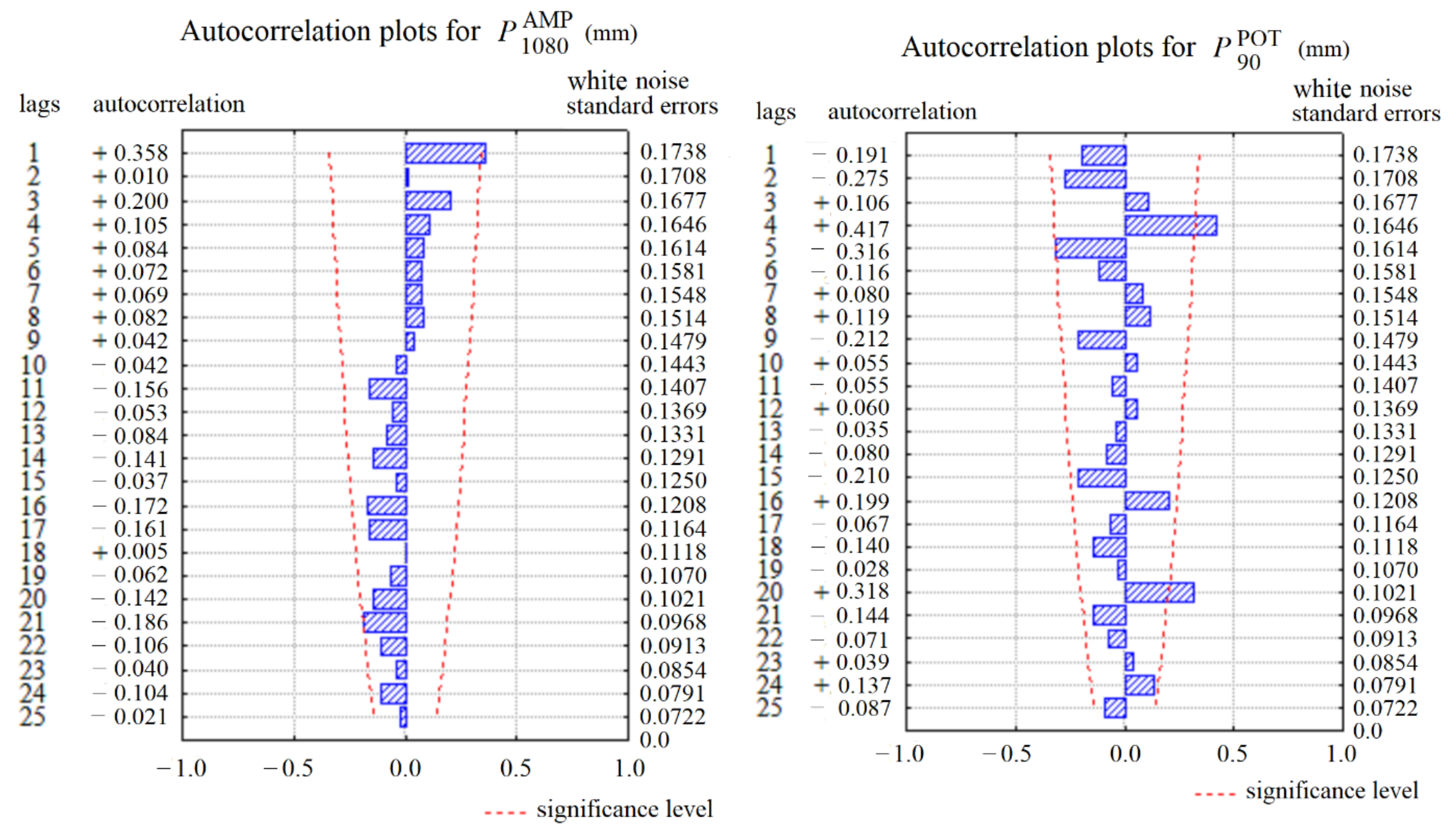
An analysis was made of the internal correlation of the series of random variables $P_{\mathsf{\tau }}^{\mathrm{AMP}}$ and $P_{\mathsf{\tau }}^{\mathrm{POT}}$ using Anderson’s test [40]. An autocorrelation analysis was performed for lags up to 25 (Figure 4). The greatest autocorrelation coefficients were detected for $P_{1080}^{\mathrm{AMP}}$ with lag = 1 (ρ = 0.358) and for $P_{90}^{\mathrm{POT}}$ with lag = 4 (ρ = 0.417). Other autocorrelation values were not large and lay within the confidence interval for the assumed significance level α = 0.05. This is a sufficient condition to conclude a lack of correlation; that is, that the analyzed random variables are independent. An analysis of the autocorrelation plots (Figure 4) also showed an absence of periodic fluctuations.

Nonhomogeneity analysis, performed using genetic and statistical methods, showed that most of the observations of maximum precipitation selected by the POT method satisfied the homogeneity requirements, except for the observations for duration τ = {10, 45, 60} min at Chojnice and τ = {15, 30, 120, 1440} min at Bialystok (Table 2 and Table 3). Most of the maximum precipitation observations selected by the AMP method are nonhomogeneous; exceptions are the $P_{\mathsf{\tau }}^{\mathrm{AMP}}$ observations from Chojnice with duration τ = 5 and τ = {720, …, 4320} min.

4.2. Computation of Maximum Precipitation with Specified Probability of Exceedance Using the PMAXTP Method

Parameters of the probability distributions of the analyzed random variables were estimated for the two adopted methods of selection of maximum precipitations, $P_{\tau }^{\mathrm{AMP}}$ and $P_{\tau }^{\mathrm{POT}}$ (for details, see Section 2). The most credible distribution was selected for the analyzed random variable by minimizing the value of the Akaike information criterion (AIC) [45]. Calculations were performed for three-parameter (α, λ or μ, ε; Equations (A1), (A3), (A5) and (A7) in Appendix A) probability distributions GA, WE, LGA, and LN, and for the two-parameter (α, μ; Equation (A9) in Appendix A) G distribution. Sample results obtained at each stage of the procedure are given in

Table 7. Sample results of the procedure to select probability distributions for maximum precipitation values $P_{\tau }^{\mathrm{AMP}}$ and $P_{\tau }^{\mathrm{POT}}$ for τ = 5 min. GA—gamma distribution; WE—Weibull; LN—log-normal; LGA—log-gamma; G—Gumbel; χ²—Pearson’s χ² goodness-of-fit test; min(D_max)—Kolmogorov’s minimum distance criterion. Bold values represent the most credible distributions according to the Akaike information criterion (AIC).

Precipitation		Probability Distribution
		Type	Parameters				χ2 ${\chi }_{\left({\alpha }_{kr}=0.05\right)}^2$ = 7.815	min(Dmax)	AIC
			α	λ	μ	ε
CHOJNICE	$P_5^{\mathrm{AMP}}$	GA	1.321	3.642	-	0.1	0.831	0.500	138.738
		WE	4.534	1.678	-	2.4	0.569	0.496	139.551
		LN	0.379	-	1.806	0.1	1.090	0.514	139.268
		LGA	0.036	113.463	-	0.1	1.182	0.552	140.164
		G	2.009	-	5.394	-	0.977	0.499	139.215
	$P_5^{\mathrm{POT}}$	GA	0.732	3.356	-	5.2	5.292	0.579	100.323
		WE	2.172	1.481	-	5.7	5.751	0.549	98.064
		LN	0.360	-	1.231	4.0	5.268	0.601	101.625
		LGA	0.048	12.131	-	4.2	5.194	0.603	101.709
		G	1.022	-	7.031	-	6.013	0.667	102.049
BIAŁYSTOK	$P_5^{\mathrm{POT}}$	GA	1.224	1.683	-	5.8	5.293	0.500	103.137
		WE	2.087	1.188	-	5.9	5.751	0.553	102.860
		LN	0.805	-	0.566	0.1	5.269	0.479	103.267
		LGA	0.107	2.967	-	5.6	5.194	0.473	102.737
		G	1.079	-	7.153	-	6.014	0.643	107.837

. The most credible theoretical probability distribution for precipitation $P_5^{\mathrm{AMP}}$ at the Chojnice station was found to be GA, while for $P_5^{\mathrm{POT}},$ it was found to be WE. At the Bialystok station, the most credible theoretical distribution for $P_5^{\mathrm{POT}}$ was determined to be LGA.

Verification of the distributions of maximum precipitation identified as most credible at the meteorological stations in Chojnice and Bialystok was performed by means of nonparametric tests of goodness of fit: D_K−S, D_A−D, D_L−S, and D_K (defined by Equations (A11)–(A14) in Appendix B). For purposes of inference, a significance level of α = 0.05 was arbitrarily selected. This is a consequence of the fact that the value of the significance level of a test is closely related to the size (length) of the random sample on whose basis the parameters of the theoretical distributions are estimated. In the present analysis, the series contained n = 30 elements, which means that the significance level can be taken to be at most α = 0.05. Verification was performed for the most credible theoretical probability distributions, which are shown in

Table 8. Results of tests of fit of the theoretical probability distributions for $P_{\tau }^{\mathrm{AMP}}$ and $P_{\tau }^{\mathrm{POT}}$, where τ = {5, 10, 15, 30, 45, 60, 90, 120, 180, 360, 720, 1080, 1440, 2160, 2880, 4320} (min). D_K−S—Kolmogorov-Smirnov test, D_A−D—Anderson-Darling test, D_L−S—Liao-Shimokawa test, D_K—Kuiper’s test, significance level α = 0.05. The value in bold type indicates rejection of the hypothesis of goodness of fit to the empirical distribution according to the statistic D_A−D at α = 0.05.

τ	CHOJNICE										BIALYSTOK
	AMP	DK−S	DA−D	DL−S	DK	POT	DK−S	DA−D	DL−S	DK	POT	DK−S	DA−D	DL−S	DK
5	GA	0.091	0.332	0.714	0.160	WE	0.100	0.472	0.819	0.195	LGA	0.086	0.323	0.764	0.168
10	-					-					LN	0.084	0.245	0.691	0.158
15	-					WE	0.117	0.268	0.668	0.206	-
30	-					WE	0.108	0.285	0.678	0.185	-
45	-					-					WE	0.078	0.259	0.647	0.155
60	-					-					WE	0.080	0.194	0.621	0.157
90	-					GA	0.150	1.098	1.199	0.278	WE	0.085	0.186	0.607	0.163
120	-					GA	0.062	0.119	0.516	0.123	-
180	-					LGA	0.087	0.155	0.537	0.155	GA	0.103	0.253	0.666	0.195
360	-					LGA	0.071	0.184	0.613	0.133	-
720	GA	0.183	0.749	1.016	0.308	LGA	0.088	0.324	0.771	0.173	WE	0.093	0.265	0.655	0.186
1080	G	0.124	0.485	0.836	0.245	WE	0.105	0.423	0.819	0.189	WE	0.091	0.263	0.677	0.161
1440	G	0.125	0.443	0.825	0.229	WE	0.109	0.286	0.676	0.172	-
2160	G	0.080	0.118	0.514	0.124	GA	0.078	0.257	0.662	0.153	WE	0.071	0.164	0.591	0.136
2880	WE	0.079	0.209	0.650	0.157	GA	0.103	0.470	0.831	0.204	WE	0.087	0.217	0.616	0.166
4320	WE	0.072	0.166	0.575	0.145	GA	0.107	0.401	0.762	0.211	WE	0.107	0.276	0.680	0.192

${\alpha }_{\mathrm{cr}.}$ = 0.05 for: D_K−Scr. = 0.242; D_A−Dcr. = 0.795; D_L−Scr. = 1.505; D_Kcr. = 0.317.

for maximum precipitation with specified duration τ, together with the results obtained in single-dimensional statistical tests and the critical values, respectively for $P_{\tau }^{\mathrm{AMP}}$ and $P_{\tau }^{\mathrm{POT}}$ at the Chojnice station and $P_{\tau }^{\mathrm{POT}}$ at Bialystok. All of the tests failed to reject the null hypothesis on the goodness of fit of the theoretical distribution with the empirical distribution, for the analyzed variables $P_{\tau }^{\mathrm{AMP}}$ and $P_{\tau }^{\mathrm{POT}}$, with the exception of the D_A−D test in relation to the maximum precipitation $P_{90}^{\mathrm{POT}}$ at Chojnice (value shown in bold type in Table 8). The least of the maximum distances between values of the theoretical and empirical cumulative probability distributions, particularly in the tail part, was situated decidedly below the critical value of the D_A−D test defined at a significance level of α = 0.05, which signifies rejection of the hypothesis of the goodness of fit of the theoretical and empirical distributions.

The results obtained from the PMAXTP model for the values of maximum precipitation with a specified probability of exceedance were compared with the results from the Bogdanowicz-Stachý model [1,2]. In the latter model, the procedure for computing the values of maximum precipitation with a specified probability of exceedance p consisted of:

(i)

regionalization of maximum precipitation;

(ii)

estimation of parameters of the probability distribution function depending on the identified region and selected duration.

The procedure of the Bogdanowicz-Stachý model conforms to the recommendations of the World Meteorological Organization [61]. The input data originated from 20 meteorological stations situated in latitudinal strips running along the coast, lake districts, lowland parts, and southern upland parts of Poland. Mountain areas were omitted, due to the absence of stations monitoring precipitation at all altitudes. The maximum quantity of precipitation with a specified duration and specified probability of exceedance was determined using the formula (A16) in Appendix C, taking account of the regionalization of the meteorological stations in Chojnice and Bialystok.

Quantile values determined using the PMAXTP and Bogdanowicz-Stachý models were compared using statistical and graphical measures. According to the regionalization carried out by Bogdanowicz and Stachý, the Chojnice meteorological station belongs to the north-west region for precipitation with durations in the range <5, >60 min, to the central region for durations in the range <60, >720 min, and to the southern/coastal region for durations in the range <720, >4320 min. The Bialystok station, located in the north-east of Poland, belongs to the central region irrespective of the duration of precipitation being considered.

For a comparison of the results given by the two models, i.e., PMAXTP and Bogdanowicz-Stachý, various statistical measures can be used [62]. In our study, we used the standard error of fit S(E), which is shown in

Table 9. Comparison of the PMAXTP and Bogdanowicz-Stachý methods for $P_{\tau }^{\mathrm{AMP}}$ and $P_{\tau }^{\mathrm{POT}}$, where τ = {5, 10, 15, 30, 45, 60, 90, 120, 180, 360, 720, 1080, 1440, 2160, 2880, 4320} (min), using the standard error of fit S(E). The comparison refers to the maximum precipitation values computed for the meteorological station in Chojnice ($P_{\tau }^{\mathrm{AMP}}$ and $P_{\tau }^{\mathrm{POT}}$) and in Bialystok ($P_{\tau }^{\mathrm{POT}}$). Values in bold type are the smallest errors S(E) obtained separately for the Chojnice and Bialystok stations.

τ	CHOJNICE								BIAŁYSTOK
	PMAXTP				B&S				PMAXTP		B&S
	AMP		POT		AMP		POT		POT		POT
	Distrib.	S(E)	Distrib.	S(E)	Distrib.	S(E)	Distrib.	S(E)	Distrib.	S(E)	Distrib.	S(E)
5	GA	0.484	WE	0.263	WE	0.801	WE	1.380	LGA	0.780	WE	2.139
10									LN	0.639	WE	2.613
15			WE	0.742			WE	2.135
30			WE	1.418			WE	2.654
45									WE	0.778	WE	3.037
60									WE	0.737	WE	3.902
90			GA	1.992			WE	4.761	WE	1.133	WE	4.424
120			GA	1.325			WE	5.469
180			LGA	1.558			WE	5.557	GA	1.999	WE	5.209
360			LGA	2.902			WE	6.095
720	GA	4.113	LGA	4.236	WE	7.246	WE	7.713	WE	2.869	WE	5.854
1080	G	3.341	WE	3.287	WE	8.441	WE	7.814	WE	2.610	WE	6.280
1440	G	3.359	WE	2.847	WE	10.430	WE	8.588
2160	G	2.924	GA	2.383	WE	11.139	WE	8.866	WE	3.543	WE	7.704
2880	WE	3.083	GA	2.761	WE	12.845	WE	10.442	WE	3.646	WE	8.593
4320	WE	2.720	GA	2.738	WE	14.218	WE	11.486	WE	4.648	WE	11.634

. The error is given by the following formula [63]:

$$\mathrm{S}\left(E\right) =\sqrt{ \begin{array}{c}{\displaystyle {\displaystyle \sum }_{i=1}^{i=m}}\left(P_{{\tau }_i}^{\mathrm{M}\mathrm{A}\mathrm{X}}-{\widehat{P}}_{{\tau }_i}^{\mathrm{M}\mathrm{A}\mathrm{X}}\right)\\ \overline{ m-l }\end{array}}$$

(1)

where $P_{\tau ,i}^{\mathrm{MAX}}$ is the observed maximum precipitation selected by the AMP or POT method for a specified duration (τ); ${\widehat{P}}_{\tau ,i}^{\mathrm{MAX}}$ is the estimated maximum precipitation from the PMAXTP or Bogdanowicz-Stachý model; m = 30 is the size of the random sample formed from empirical quantiles for m = 30 selected probabilities p $\in$ {96.8, 93.6, 90.3, 87.1, 83.9, 80.7, 77.4, 74.2, 70.9, 67.7, 64.5, 61.3, 58.1, 54.8, 51.6, 48.4, 45.2, 41.9, 38.7, 35.5, 32.3, 29.0, 25.8, 22.6, 19.4, 16.1, 12.9, 9.7, 6.5, 3.2} % and the corresponding theoretical distributions computed using the PMAXTP and Bogdanowicz-Stachý methods. Finally, l is the number of parameters of the theoretical probability distribution according to the density function (Equations (A1), (A3), (A5), (A7) and (A9) in Appendix A).

Computations of the error S(E) were performed separately for specified durations τ of maximum precipitation. The value of the standard error of fit increased with increasing values of τ for both models. The smallest errors were obtained for the quantiles determined from the maximum precipitation values selected using the POT method and the PMAXTP model. An exception was the quantiles determined for the AMP values at the Chojnice station for duration τ equal to 720 and 4320 min. The errors of fit of the theoretical to the empirical distributions in the Bogdanowicz-Stachý model for precipitation values selected by the AMP method were on average 210% greater than those obtained with the PMAXTP model, and for the POT precipitation values, the errors were 300% greater. The most frequently selected most credible theoretical probability distribution for random samples of both AMP and POT maximum precipitation values, and for both the Bialystok and the Chojnice stations, was the WE distribution.

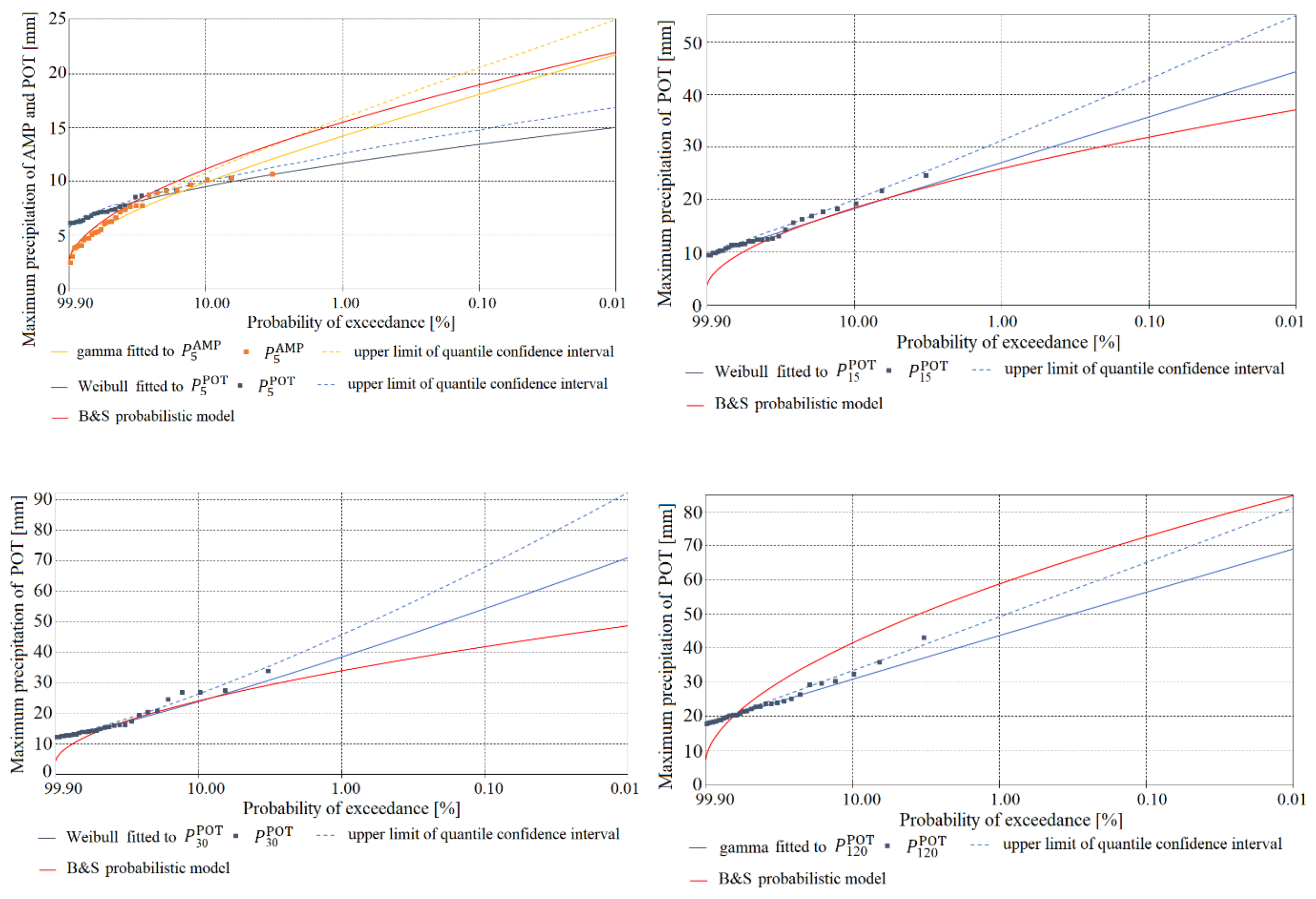
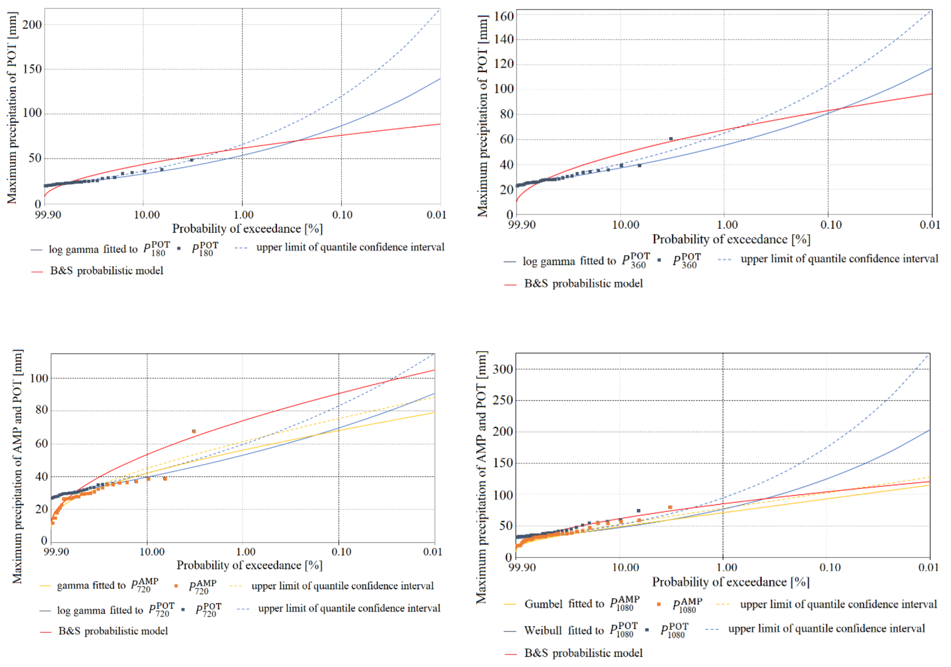
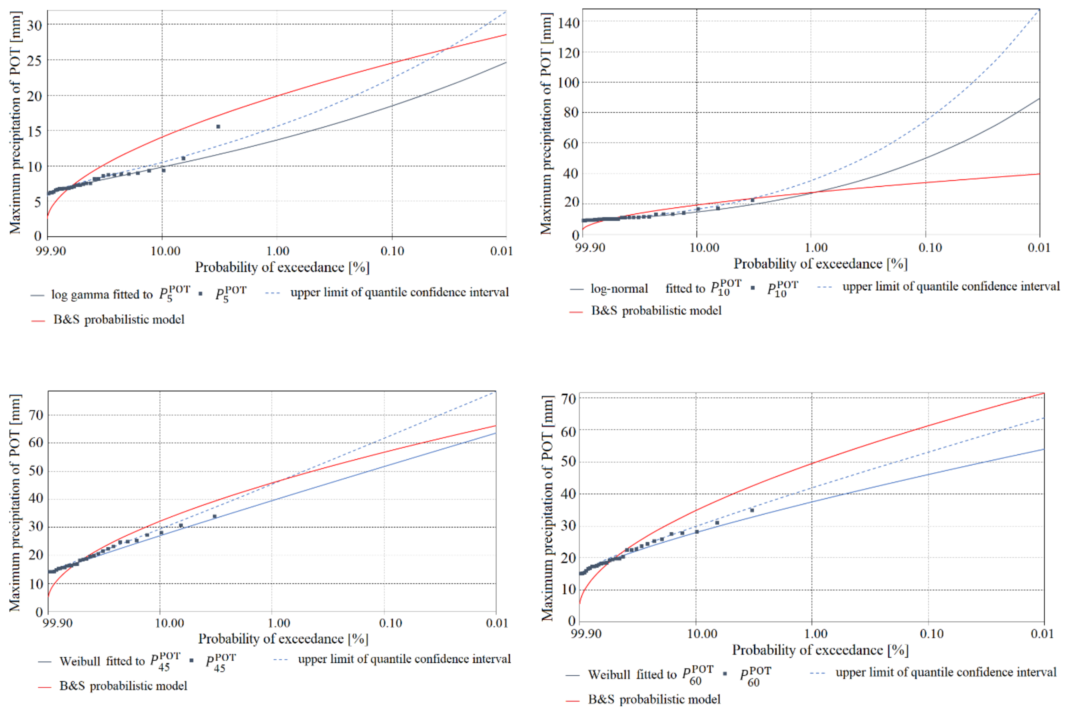
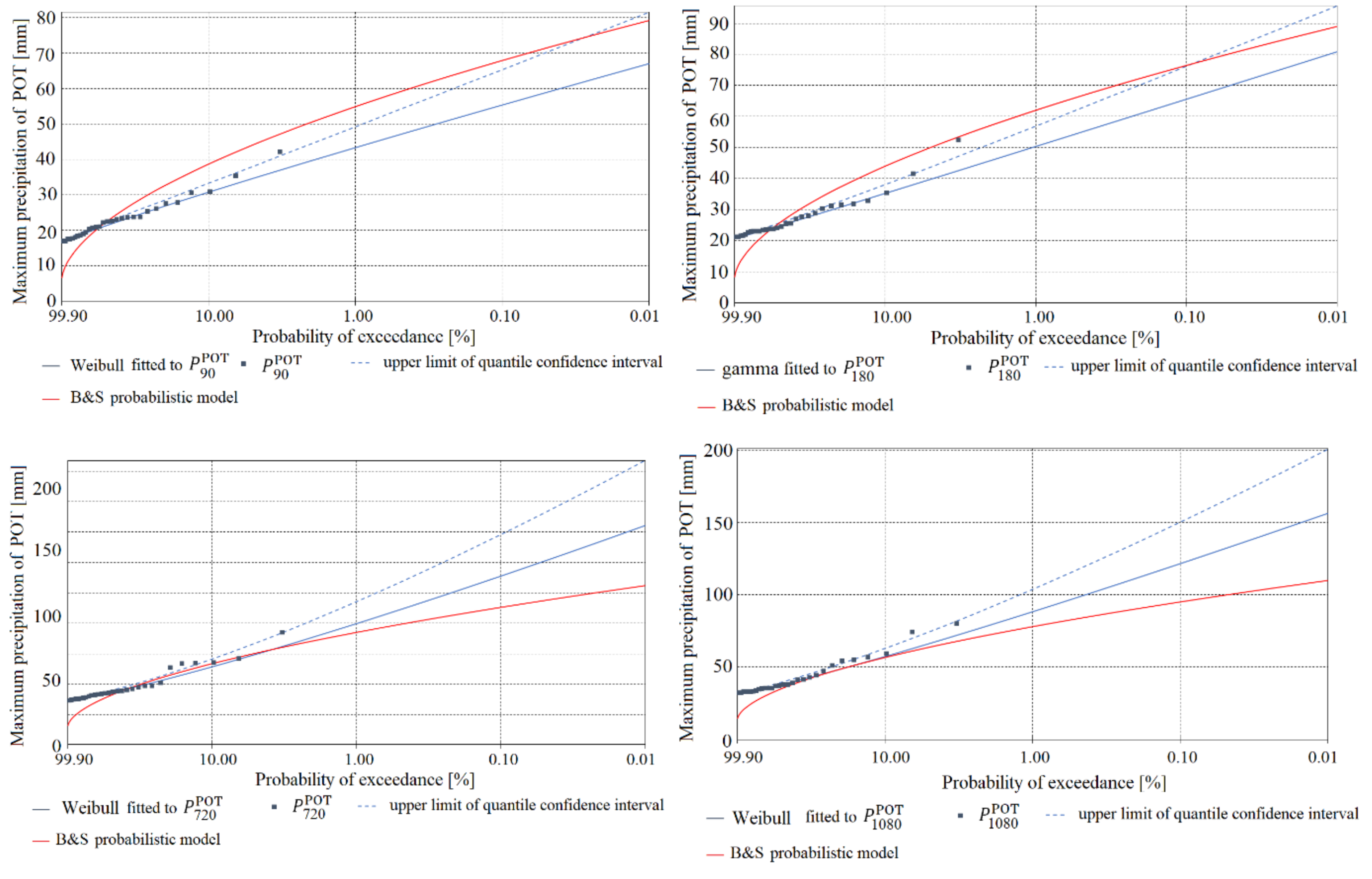
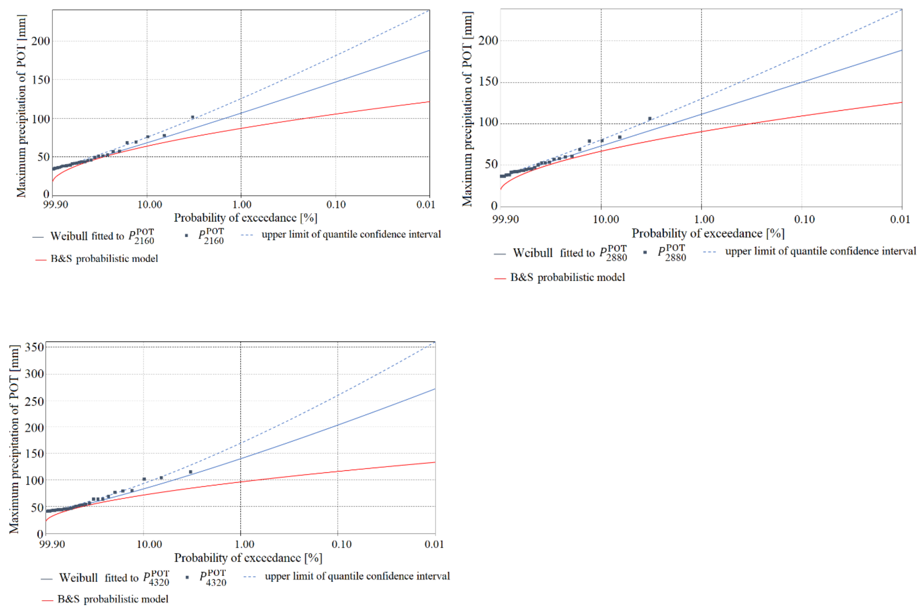
Figure 5, Figure 6, Figure 7, Figure 8, Figure 9 and Figure 10 show a comparison of the functions for the probability of exceedance of maximum precipitations $P_{\tau }^{\mathrm{AMP}}$ or $P_{\tau }^{\mathrm{POT}}$ determined using the models, for Chojnice (Figure 5, Figure 6 and Figure 7) and Bialystok (Figure 8, Figure 9 and Figure 10). The plots contain density functions of probability distributions computed only for homogeneous observations of precipitation selected by the AMP and POT methods, in accordance with the results shown in Table 2, Table 3 and Table 8. The diagrams show comparisons of: (i) the most credible probability functions for maximum precipitation determined by the PMAXTP model for the AMP observation series (orange solid line) and for maximum precipitation selected by the POT method (blue solid line); (ii) upper limits of confidence intervals (orange and blue dotted lines); (iii) observations of AMP and POT maximum precipitation (orange and blue squares); and (iv) the probability function determined using the probabilistic Bogdanowicz-Stachý model (red solid line).

At the Chojnice station, for practically all of the analyzed durations of maximum precipitation, the quantile values from the Bogdanowicz-Stachý model are markedly higher than the observed precipitations and values of corresponding quantiles from the PMAXTP model, in relation to the maximum precipitations selected both by the AMP method (orange squares and solid line) and by the POT method (blue squares and solid line). The differences between the quantiles are particularly visible in the central region and in the region of the upper tails of the probability distributions. Similar maximum quantile values were obtained for precipitation with duration τ = {15, 30, 180, 1080} min. At Chojnice, the AMP values were described by the models GA and WE, while for description of the POT maximum precipitation values, the WE distribution was selected for short durations τ, and GA and LGA for medium and long durations.

At the Bialystok station, in the case of maximum precipitations with duration τ = {5, 45, 60, 90, 180} min (Figure 8 and Figure 9), the quantile values determined using the Bogdanowicz-Stachý model (red solid line) are markedly higher than the corresponding quantiles obtained using the PMAXTP model for the maximum precipitations determined by the POT method (blue squares and solid line). Differences between quantiles are particularly visible in the central region and in the region of the upper tails of the probability distributions. The closest results for quantiles of POT maximum precipitations calculated using the PMAXTP method and from the Bogdanowicz-Stachý model were obtained for precipitation with duration τ = {720, 1080} min (Figure 9). For maximum precipitation with such durations, the most credible theoretical distribution was WE, while for short durations, τ = {5, 10} min, the respective distributions were LGA and GA. For maximum precipitation selected by the POT method with duration τ = {2160, …, 4320} min, the Bogdanowicz-Stachý model returned markedly lower quantile values than the PMAXTP method.

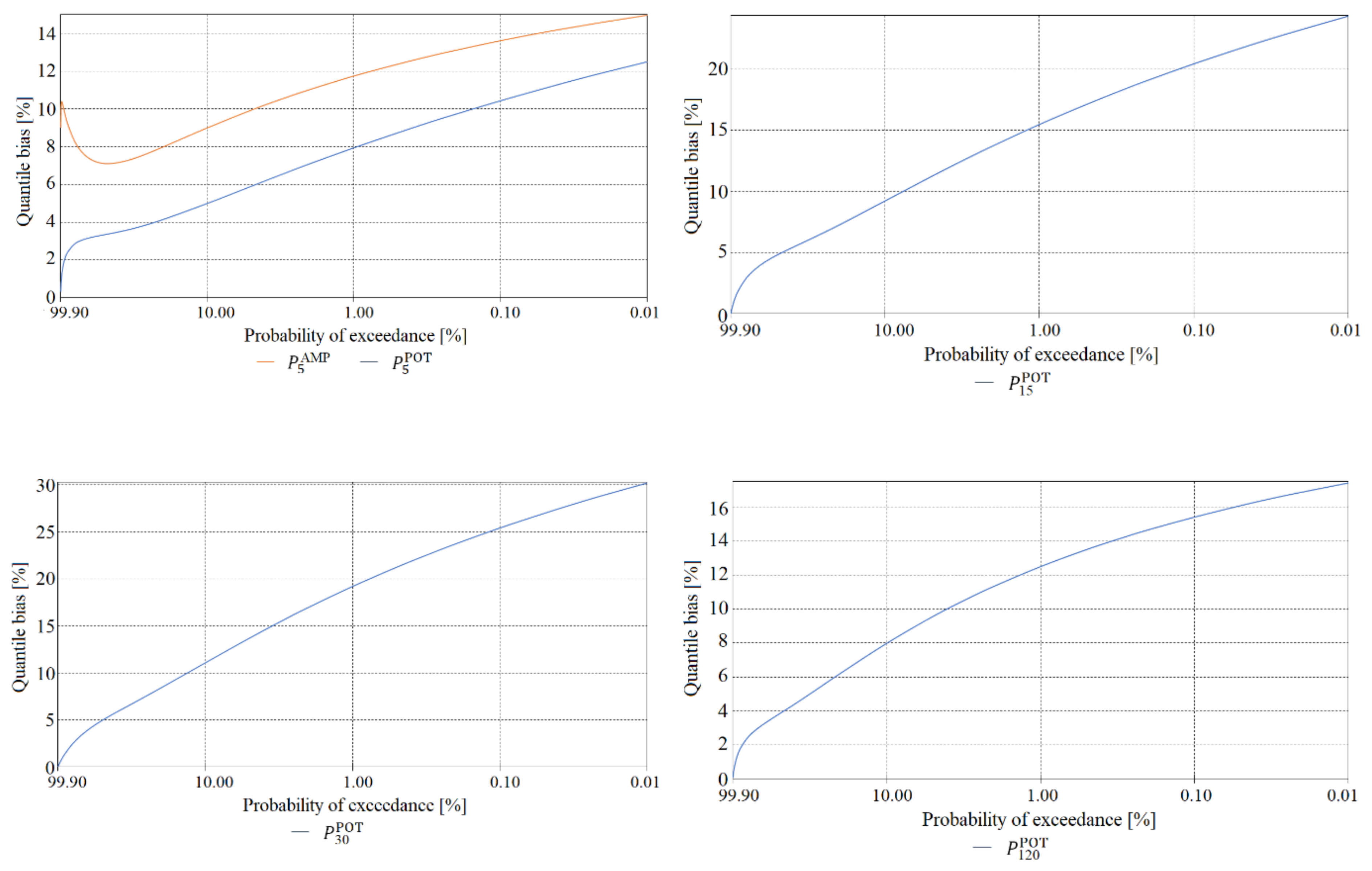
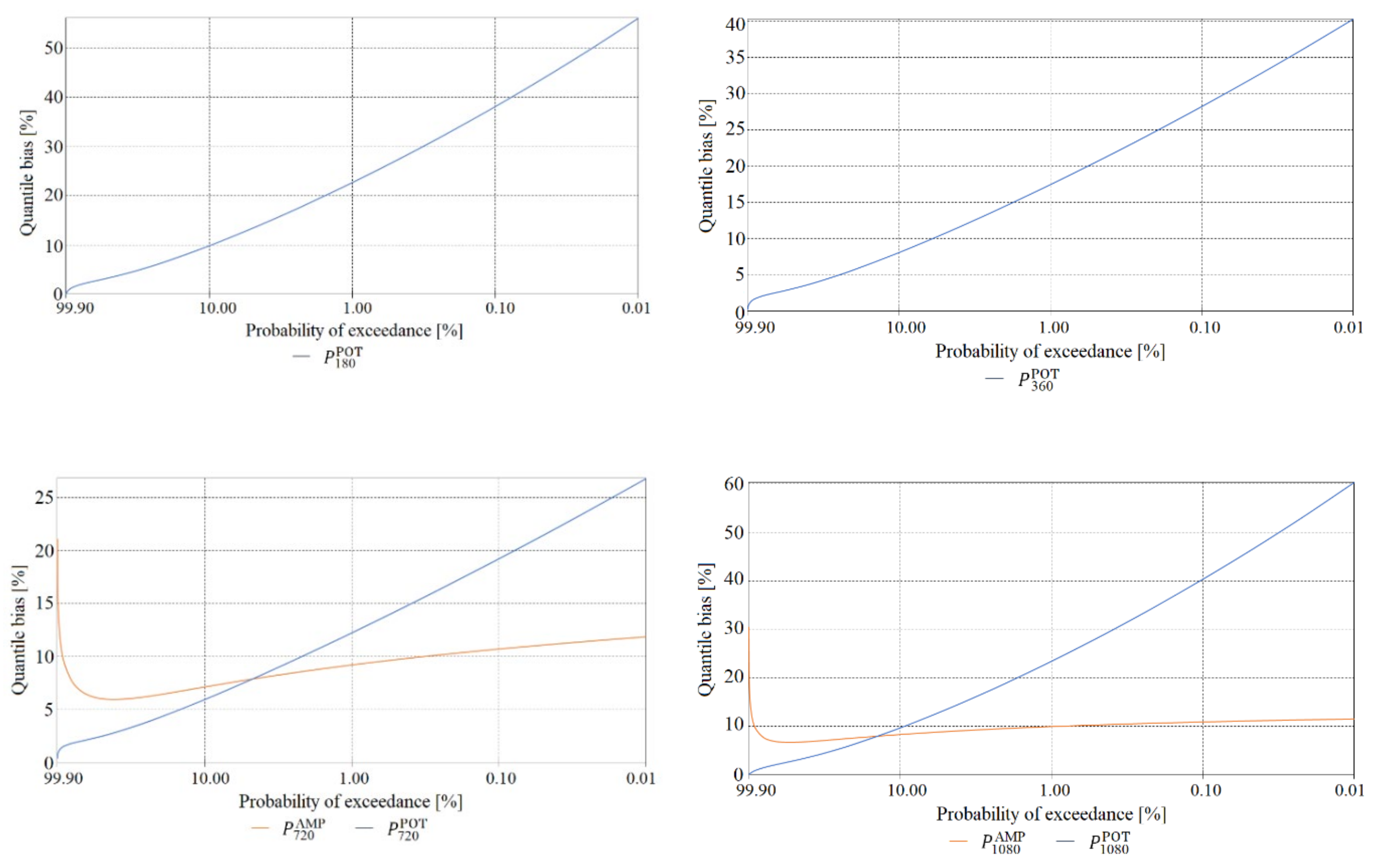
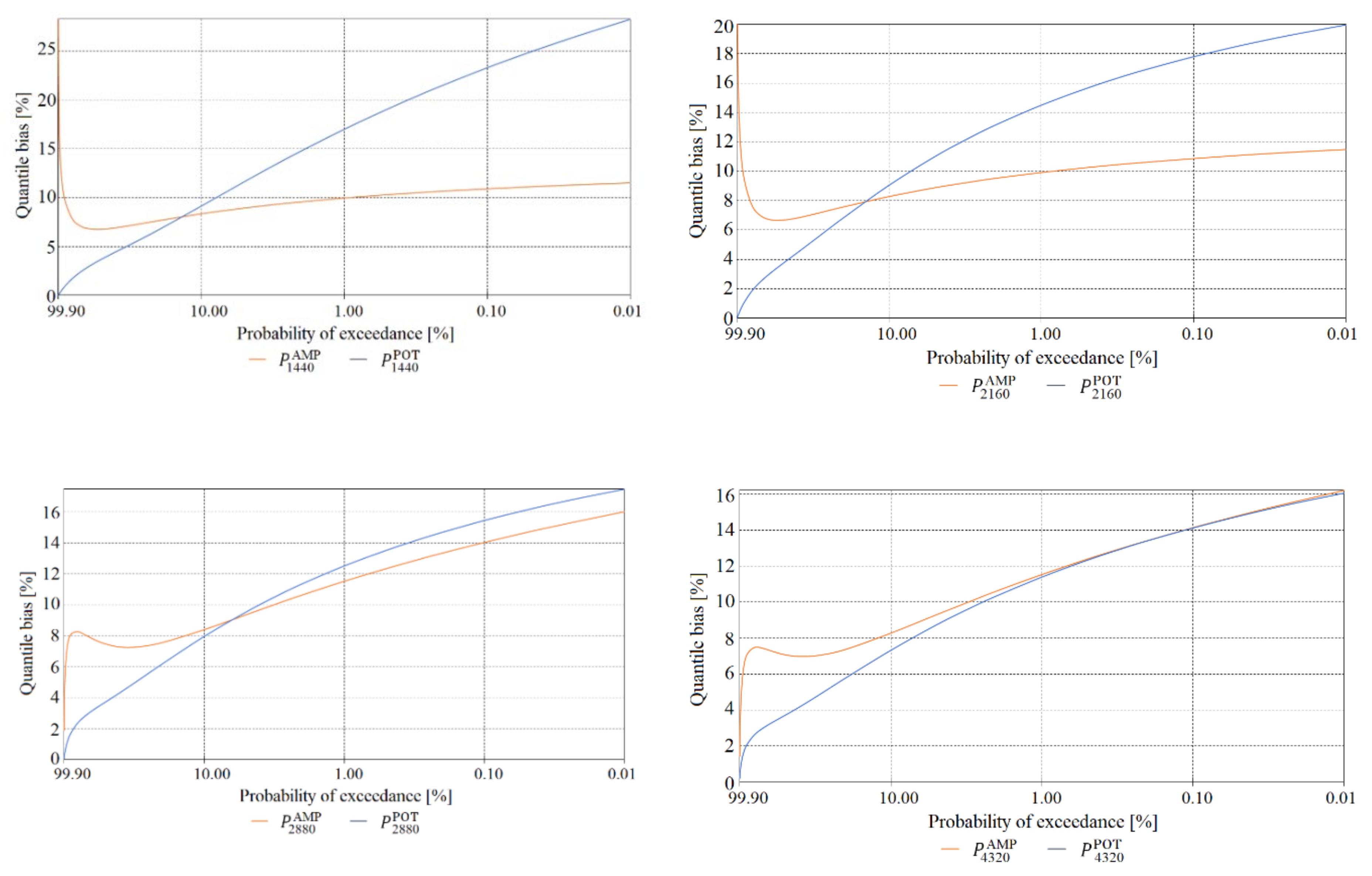
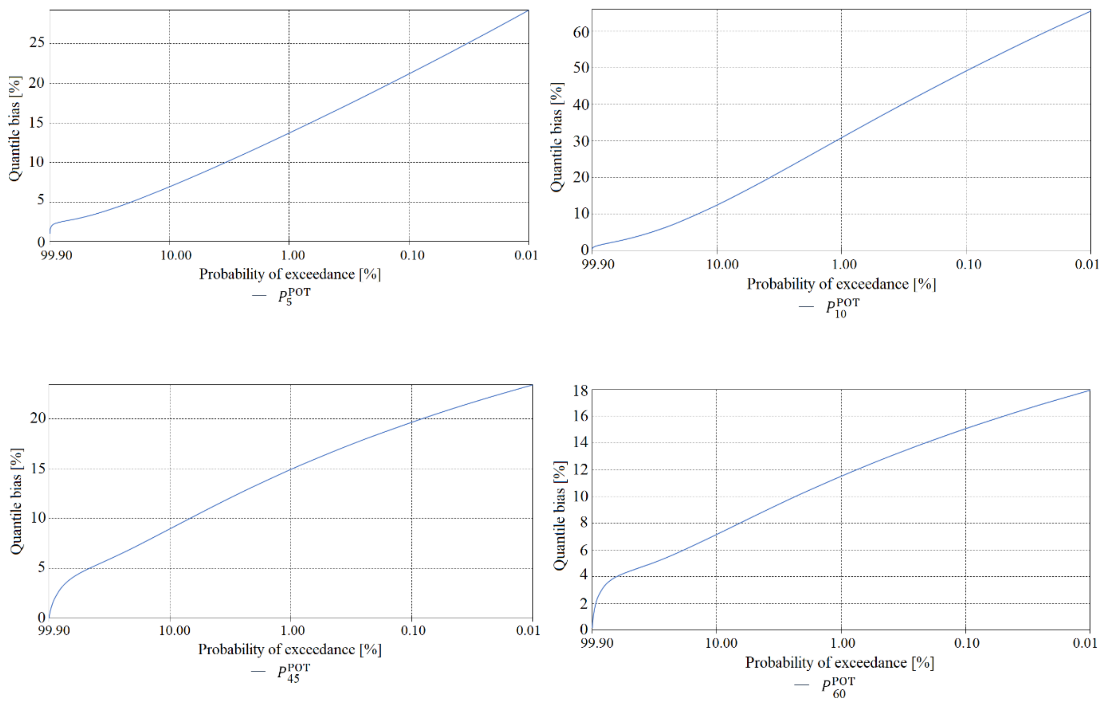
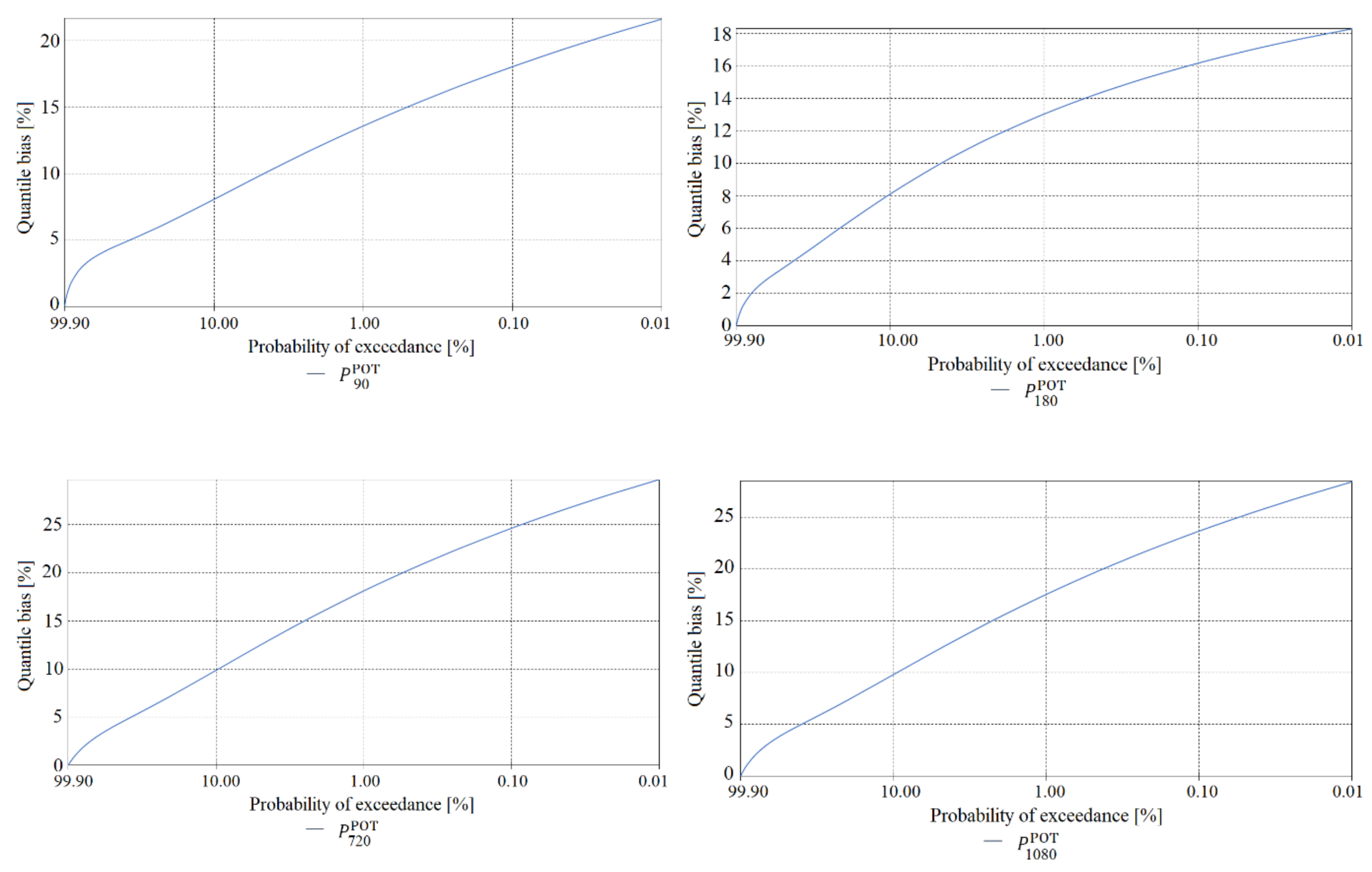
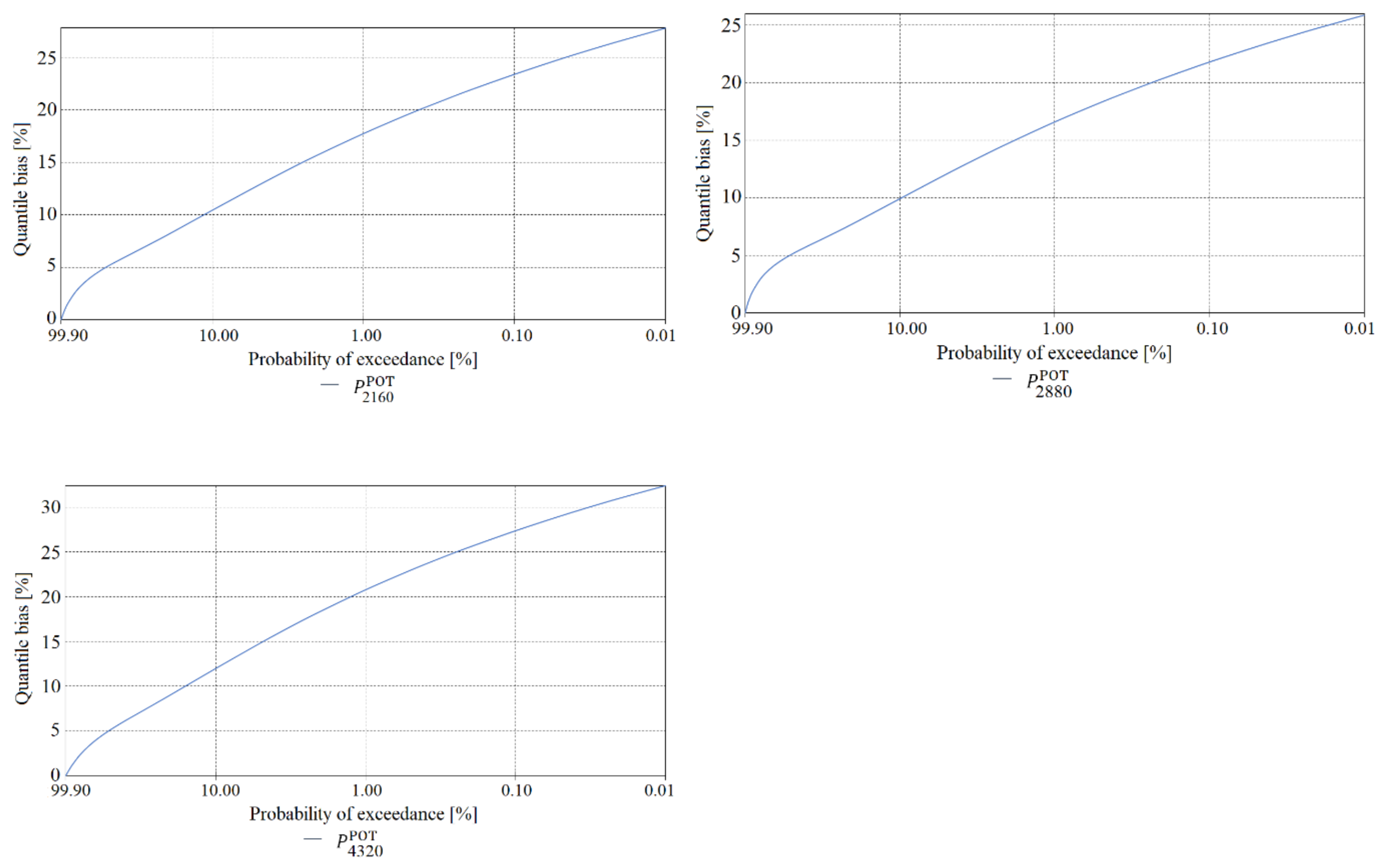
The final element of the verification of maximum precipitation values was a comparison of the estimated quantile error resulting from the randomness of the sample of maximum precipitations computed using the PMAXTP model for the random variables $P_{\tau }^{\mathrm{AMP}}$ and $P_{\tau }^{\mathrm{POT}}$ at the meteorological station in Chojnice (Figure 11, Figure 12 and Figure 13) and for $P_{\tau }^{\mathrm{POT}}$ at the meteorological station in Bialystok (Figure 14, Figure 15 and Figure 16).

The largest errors for values of maximum precipitation with high probabilities, such as 99.0 and 99.9, at the Chojnice station were observed for maximum precipitations selected using the AMP method (Figure 11 for τ = 5, Figure 12 for τ = {720, 1080}, Figure 13 for τ = {1440, …, 2160} min)—markedly higher errors for the AMP series than for the POT series at Chojnice. The largest errors for values of maximum precipitation with low probabilities, such as 0.01 and 0.001, were recorded for the Chojnice station (Figure 12 for τ = {720, 1080} and Figure 13 for τ = {1440, …, 2160} min) for POT precipitations (markedly higher errors for the POT series than for the AMP series at Chojnice). The smallest differences in the quantile error in the entire range of theoretical occurrence of maximum precipitation were observed at Chojnice (Figure 13 for τ = {2880, 4320} min).

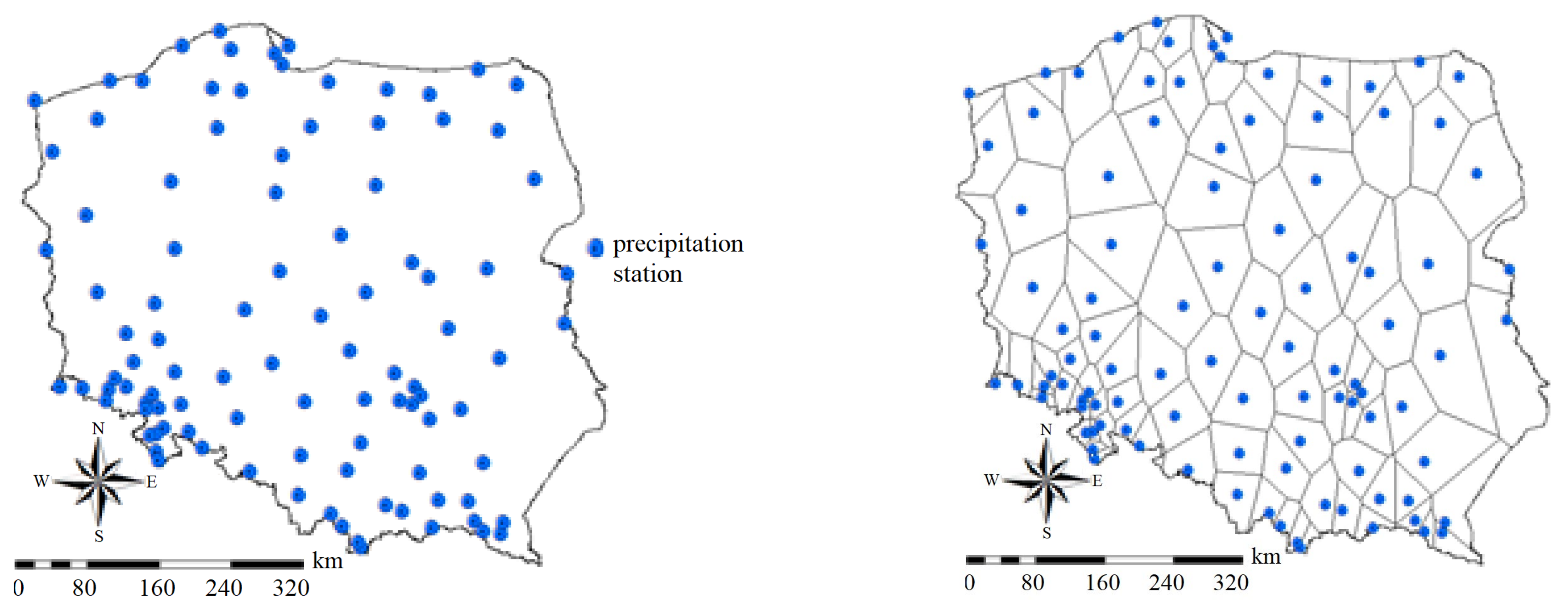
Calculations were made for 100 total rainfall measuring sites in Poland (Figure 17). Calculated characteristics of maximum rainfall totals, i.e., quantile values for p(%) ∈ {99.9, 99.5, 99, 98.5, 98, 95, 90, 80, 70, 60, 50, 40, 30, 20, 10, 5, 3, 2, 1, 0.5, 0.3, 0.2, 0.1, 0.05, 0.03, 0.02, 0.01} of a specified duration, τ(min) ∈ {5, 10, 15, 30, 45, 60, 90, 120, 180, 360, 720, 1080, 1440, 2160, 2880, 4320}, upper limits of the confidence interval and quantile errors were interpolated by the Thiessen Polygons (TP) method, which allowed for the assignment of certain areas for which measuring sites are representative as well as for the proportional division and distribution of sites within Poland. Higher resolution calculations can be achieved using Gaussian geostatistical simulation models [64] that accept any simple kriging model [65] or residual kriging model [66].

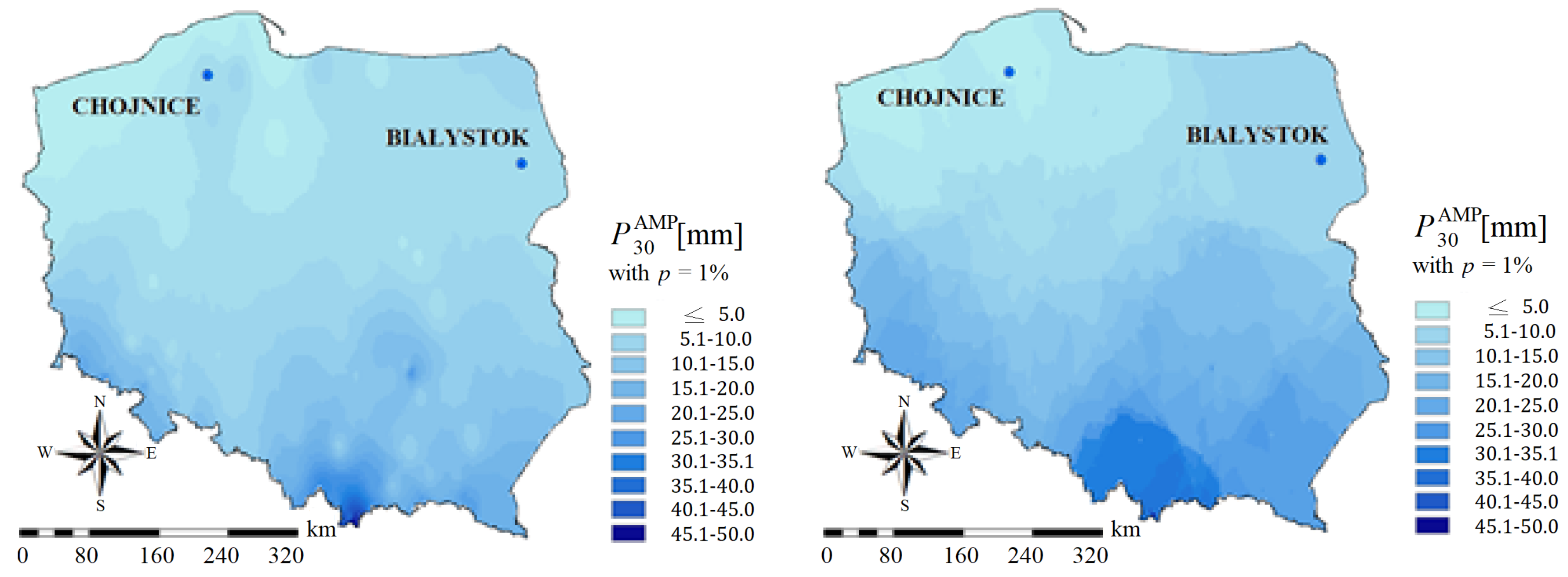
Interpolation also can be performed using the Inverse Distance Weighted (IDW) method, which uses a linearly weighted set of sampling points to determine mesh node values by using reverse weighted distance values. The weight is a function of the inverse distance, and the interpolated surface should be a variable surface depending on the position of the point [67]. An example of interpolating the maximum precipitation value $P_{\tau }^{\mathrm{AMP}}$ with a duration of τ = 30 min with a probability p = 1% calculated using the IDW method is shown in Figure 18 (left part).

The IDW is a deterministic interpolation method because it is directly based on surrounding measured values. Another example is the set of geostatistical methods, such as the Kriging methods (right part of Figure 18), which include autocorrelation, which represents the statistical relationship between the measured points, thus providing a certain measure of reliability or accuracy of the forecast. The Kriging method is most suitable when one knows that there is spatial distance correlation or directional deviation in the data being analyzed.

5. Conclusions

This paper described the PMAXTP model for a frequency analysis of maximum precipitation with a specified duration. It consists of two modules: statistical and computational. The first step selects values of maximum precipitation of a specified duration, which is conducted using two different methods: Annual Maximum Precipitation (AMP) and Peaks-Over-Threshold (POT). The advantage of the POT method is that it selects a larger number of observations of precipitation with the highest values in a given year, which leads to a better estimation of the characteristics of maximum precipitation with a specified duration and probability of exceedance. This is a significant issue in the design of drainage structures, particularly when they are at high risk of damage. The statistical module enables an analysis of the homogeneity of the series of measurements of maximum precipitation that serve as the input to the computational module, in which the mathematical models used for parameter estimation require a simple random sample, that is, one that satisfies the assumptions of independence and stationarity.

The computational module enables the selection of the best (the most credible) theoretical probability distribution by means of: (i) estimation of the parameters of four types of distributions belonging to the families gamma (GA), Weibull (WE), log-gamma (LGA), log-normal (LN), and Gumbel function (G); (ii) test of the hypothesis of goodness of fit of the theoretical probability distribution function with the empirical distribution using Pearson’s χ² test; (iii) selection of the best-fitting function in each distribution type according to the criterion of minimum Kolmogorov distance; (iv) selection of the most credible distribution function from the set of best-fitting functions of various types; and (v) verification of the most credible distributions of precipitations $P_{\tau }^{\mathrm{AMP}}$ and $P_{\tau }^{\mathrm{POT}}$ using the single-dimensional tests D_K−S, D_A−D, D_L−S, and D_K.

The PMAXTP model was tested on data from two meteorological stations in Poland (Chojnice and Bialystok) representing two regions characterized by different spatial variability of maximum precipitation. The results were compared with those given by the Bogdanowicz-Stachý model—which to date has frequently been used in engineering practice in Poland—based on estimated values of the quantile error resulting from the randomness of the sample of maximum precipitation values computed for the tested stations.

In general, the errors of fit for the theoretical to the empirical distribution for the PMAXTP model were lower than the errors for the Bogdanowicz-Stachý model. The smallest errors were obtained for the quantiles determined on the basis of maximum precipitation POT using the PMAXTP model for both analyzed stations.

The following detailed conclusions may be drawn from the results:

• Most of the observations of maximum precipitation selected by the POT method satisfied the requirement of homogeneity, with the exception of the observations with durations τ = {10, 45, 60} min at Chojnice and τ = {15, 30, 120, 1440} min at Bialystok.
• Most of the observations selected by the AMP method did not satisfy the requirement of homogeneity, with the exception of the observations with durations τ = 5 min and τ = {720, …, 4320} min at Chojnice.
• Errors of fit of the theoretical to the empirical distributions for the Bogdanowicz-Stachý model were on average 210% higher than the errors for the PMAXTP model in the case of the precipitation $P_{\tau }^{\mathrm{AMP}}$, and 300% higher in the case of $P_{\tau }^{\mathrm{POT}}$.
• The smallest errors were obtained for the quantiles determined on the basis of observations of maximum precipitation $P_{\tau }^{\mathrm{POT}}$ obtained using the PMAXTP model.
• For the meteorological station in Chojnice, practically all of the quantile values determined by the Bogdanowicz-Stachý model were markedly higher than those obtained by the PMAXTP model and the quantiles of the empirical precipitations $P_{\tau }^{\mathrm{AMP}}$ and $P_{\tau }^{\mathrm{POT}}$, while for the station in Bialystok, the Bogdanowicz-Stachý model gave higher quantile values for τ = {5, …, 180} min and markedly lower values for τ = {2160, …, 4320} min.
• The greatest errors for the low quantiles, i.e., the values of maximum precipitation that are exceeded with high probability, were observed for the precipitation values for $P_{\tau }^{\mathrm{AMP}}$, and the greatest errors for high quantiles, i.e., the values of maximum precipitation that are exceeded with low probability, were observed for the precipitation values for $P_{\tau }^{\mathrm{POT}}$.

References

- Salas, J.D.; Obeysekera, J. Revisiting the concepts of return period and risk for nonstationary hydrologic extreme events. J. Hydrol. Eng. 2014, 19, 554–568. [Google Scholar] [CrossRef] [Green Version]
- Derbile, E.K.; Kasei, R.A. Vulnerability of crop production to heavy precipitation in north-eastern Ghana. Int. J. Clim. Chang. Strateg. Manag. 2012, 4, 36–53. [Google Scholar] [CrossRef]
- Tian, Q.; Li, Z.; Sun, X. Frequency analysis of precipitation extremes under a changing climate: A case study in Heihe River basin, China. J. Water Clim. Chang. 2020, 12, 772–786. [Google Scholar] [CrossRef] [Green Version]
- Lazoglou, G.; Anagnostopoulou, C. An Overview of Statistical Methods for Studying the Extreme Rainfalls in Mediterranean. Proceedings 2017, 1, 4132. [Google Scholar] [CrossRef] [Green Version]
- Acero, F.J.; Parey, S.; Garcia, J.A.; Dacunha-Castelle, D. Return Level Estimation of Extreme Rainfall over the Iberian Peninsula: Comparison of Methods. Water 2018, 10, 179. [Google Scholar] [CrossRef] [Green Version]
- Jenkinson, A.F. The frequency distribution of the annual maximum (or minimum) of meteorological elements. Q. J. R. Meteorol. Soc. 1955, 81, 158–171. [Google Scholar] [CrossRef]
- Lee, S.H.; Maeng, S.J. Frequency analysis of extreme rainfall using L-moment. Irrig. Drain. 2003, 52, 219–230. [Google Scholar] [CrossRef]
- Ahmed, A.O.M.; Al-Kutubi, H.S.; Ibrahim, N.A. Comparison of the Bayesian and maximum likelihood estimation for Weibull Distribution. J. Math. Stat. 2010, 6, 100–104. [Google Scholar] [CrossRef]
- Teimouri, M.; Nadarajah, S. Comparison of Estimation methods for the Weibull distribution. Stat. J. Theor. Appl. Stat. 2011, 47, 93–109. [Google Scholar] [CrossRef]
- Ragulina, G.; Reitan, T. Generalized extreme value shape parameter and its nature for extreme precipitation using long time series and the Bayesian approach. Hydrol. Sci. J. 2017, 62, 863–879. [Google Scholar] [CrossRef]
- Yuan, J.; Emura, K.; Farnham, C.; Alam, M.A. Frequency analysis of annual maximum hourly precipitation and determination of best fit probability distribution for regions in Japan. Urban Clim. 2018, 24, 276–286. [Google Scholar] [CrossRef]
- Młyński, D.; Wałęga, A.; Petroselli, A.; Tauro, F.; Cebulska, M. Estimating Maximum Daily Precipitation in the Upper Vistula Basin, Poland. Atmosphere 2019, 10, 43. [Google Scholar] [CrossRef] [Green Version]
- Katz, R.W.; Parlang, M.B. Naveau, Statistics of extremes in hydrology. Adv. Water Resour. 2002, 25, 1287–1304. [Google Scholar] [CrossRef] [Green Version]
- Adlouni, S.E.; Ouarda, T.B.M.J.; Zhang, X.; Roy, R.; Bobée, B. Generalized maximum likelihood estimators for the nonstationary generalized extreme value model. Water Resour. Res. 2005, 43, 6–13. [Google Scholar] [CrossRef]
- Bogdanowicz, E.; Stachý, J. Maksymalne Opady Deszczu w Polsce—Charakterystyki Projektowe (Maximum Rainfalls in Poland—Design Values); Instytut Meteorologii i Gospodarki Wodnej: Warszawa, Poland, 1998; Volume 23, pp. 55–75. [Google Scholar]
- Bogdanowicz, E.; Stachý, J. Maximum Rainfall in Poland—A Design Approach. In Proceedings of the Symposium on the Extremes of the Extremes: Extraordinary Floods, Reykjavik, Iceland, July 2000; pp. 15–18. Available online: https://www.researchgate.net/publication/295420771_Maximum_rainfall_in_Poland_-_A_design_approach (accessed on 22 September 2021).
- Shahzadi, A.; Akhter, A.S.; Saf, B. Regional Frequency Analysis of Annual Maximum Rainfall in Monsoon Region of Pakistan using L-moment. Pak. J. Stat. Oper. Res. 2015, 9, 111–136. [Google Scholar] [CrossRef] [Green Version]
- Raynal-Villasenor, J.A. Maximum likelihood parameter estimators for the two populations GEV distributions. IJRRAS 2012, 11, 350–357. [Google Scholar]
- Alila, Y.; Mtiraoui, A. Implications of heterogeneous flood-frequency distributions on traditional stream-discharge prediction techniques. Hydrol. Process. 2002, 16, 1065–1084. [Google Scholar] [CrossRef]
- Evin, G.; Merleau, J.; Perreault, L. Two-component mixture of normal, gamma and Gumbel distributions for Hydrological applications. Water Resour. Res. 2011, 47, W08525. [Google Scholar] [CrossRef]
- Shin, J.Y.; Lee, T.; Ouarda, T.B. Heterogeneous Mixture Distributions for Modeling Multisource Extreme Rainfalls. J. Hydrometeorol. 2015, 16, 2639–2656. [Google Scholar] [CrossRef]
- Rulfová, Z.; Buishand, A.; Roth, M.; Kyselý, J. A two-component generalized extreme value distribution for precipitation frequency analysis. J. Hydrol. 2016, 534, 659–668. [Google Scholar] [CrossRef]
- Kleiber, W.; Katz, R.W.; Rajagopalan, B. Daily spatiotemporal precipitation simulation using latent and transformed Gaussian Processes. Water Resour. Res. 2012, 48, W01523. [Google Scholar] [CrossRef] [Green Version]
- Evin, G.; Favre, A.-C. A new rainfall model based on the Neyman-Scott process using cubic copulas. Water Resour. Res. 2008, 44. [Google Scholar] [CrossRef] [Green Version]
- Gyasi-Agyei, Y. Copula-based daily rainfall disaggregation model. Water Resour. Res. 2011, 47, W07535. [Google Scholar] [CrossRef]
- Vernieuwe, H.; Vandenberghe, S.; De Baets, B.; Verhoest, N.E.C. A continuous rainfall model based on vine copulas. Hydrol. Earth Syst. Sci. 2015, 19, 2685–2699. [Google Scholar] [CrossRef] [Green Version]
- Strupczewski, W.G.; Singh, V.P.; Feluch, W. Non-stationary approach to at-site flood frequency modelling. Part I. Maximum likelihood estimation. J. Hydrol. 2001, 248, 123–142. [Google Scholar] [CrossRef]
- Strupczewski, W.G.; Singh, V.P.; Mitosek, H.T. Non-stationary approach to at-site flood frequency modelling. Part III. Flood analysis of Polish rivers. J. Hydrol. 2001, 248, 152–167. [Google Scholar] [CrossRef]
- Villarini, G.; Smith, J.A.; Napolitano, F. Nonstationary modelling of a long record of rainfall and temperature over Rome. Adv. Water Resour. 2010, 33, 1256–1267. [Google Scholar] [CrossRef]
- Lopez, J.; Frances, F. Non-stationary flood frequency analysis in continental Spanish rivers, using climate and reservoir indices as external covariates. Hydrol. Earth Syst. Sci. 2013, 17, 3189–3203. [Google Scholar] [CrossRef] [Green Version]
- Cheng, L.; AghaKouchak, A.; Gilleland, E.; Katz, R.W. Nonstationary extreme value analysis in a changing climate. Clim. Chang. 2014, 127, 353–369. [Google Scholar] [CrossRef]
- Zhang, D.; Yan, D.; Wang, Y.C.; Lu, F.; Liu, S. GAMLSS—based nonstationary modeling of extreme precipitation in Beijing-Tianjin-Hebei region of China. Nat. Hazards 2015, 77, 1037–1053. [Google Scholar] [CrossRef]
- Debele, S.E.; Strupczewski, W.G.; Bogdanowicz, E. A comparison of three approaches to non-stationary flood frequency analysis. Acta Geophys. 2017, 65, 863–883. [Google Scholar] [CrossRef]
- Serinaldi, F.; Kilsby, C.G. Stationarity is undead: Uncertainty dominates the distribution of extremes. Adv. Water Resour. 2015, 77, 17–36. [Google Scholar] [CrossRef] [Green Version]
- Ozga-Zielinska, M.; Ozga-Zielinski, B.; Brzezinski, J. Guidelines for Flood Frequency Analysis—Long Measurement Series of River Discharge; Institute of Meteorology and Water Management (IMGW-PIB): Warszawa, Poland, 2005; Volume 44, Available online: https://serc.carleton.edu/hydromodules/steps/168500.html (accessed on 22 September 2021).
- Ozga-Zieliński, B. Metody analizy niejednorodności ciągów pomiarowych zjawisk hydrologicznych (Methods of nonhomogeneity analysis of measurement series of hydrological phenomena). Wiadomości Instututu Meteorologii Gospodarki Wodnej 1999, 22, 13–32. [Google Scholar]
- Spearman, C. The proof and measurement of association between two thigs. Am. J. Psychol. 1904, 1, 45–58. [Google Scholar] [CrossRef]
- Pearson, F.R.S.K. On the inheritance of mental disease. Ann. Hum. Genet. 1931, 4, 362–380. [Google Scholar] [CrossRef]
- Box, G.E.P. Non-normality and tests on variances. Biometrika 1953, 40, 318–335. [Google Scholar] [CrossRef]
- Anderson, R.L. Distribution of the serial correlation coefficient. Ann. Math. Statist. 1941, 8, 1–13. [Google Scholar] [CrossRef]
- Ciupak, M.; Ozga-Zielinski, B.; Brzezinski, J. FFA and PFA Software, Version 1.1. Eng, Available Free of Charge on Demand from authors by email [email protected] or [email protected]; Institute of Meteorology and Water Management: Warsaw, Poland, 2019.
- Chapra, S.; Canale, R. Numerical Methods for Engineers, 5th ed.; McGraw-Hill Science/Engineering/Math: New York, NY, USA, 2006; p. 960. [Google Scholar]
- Neyman, J. Contributions to the Theory of the χ2 Test. Berkeley Symposium on Mathematical Statistics and Probability; University of California Press: Berkeley, CA, USA, 1949; pp. 239–273. [Google Scholar]
- Pratt, I.W.; Gibbons, I.D. Concepts of Nonparametric Theory; Springer: New York, NY, USA, 1981. [Google Scholar] [CrossRef]
- Akaike, H. A new look at the statistical model identification. IEEE Trans. Autom. Control 1974, 19, 716–722. [Google Scholar] [CrossRef]
- Genest, C.; Rémillard, B.; Beaudoin, D. Godness-of-fit tests for copulas: A review and power study. Insur. Math. Econ. 2009, 44, 199–213. [Google Scholar] [CrossRef]
- Homaei, F.; Najafzadeh, M. A reliability—Based probabilistic evaluation of the wave-induced scour depth around marine structure piles. Ocean Eng. 2020, 196, 106818. [Google Scholar] [CrossRef]
- Anderson, T.W.; Darling, D.A. A Test of Goodness of Fit. J. Am. Stat. Assoc. 1954, 49, 765–769. [Google Scholar] [CrossRef]
- Liao, M.; Shimokawa, T. A new goodness-of-fit test for Type—I extreme value and 2-parameter Weibull distributions with estimated parameters. J. Stat. Comput. Simul. 1999, 64, 23–48. [Google Scholar] [CrossRef]
- Koziol, J.A. A weighted Kuiper statistic for goodness of fit. Stat. Neerl. 2008, 50, 394–403. [Google Scholar] [CrossRef]
- Institute of Meteorology and Water Management (IMGW-PIB). Internal Report from Completion Parts I and II of PANDa Project; Institute of Meteorology and Water Management (IMGW-PIB): Gdynia, Poland, 2017; Volume I. (In Polish) [Google Scholar]
- Nguyen, T.-H.; Outayek, S.E.; Lim, S.H.; Nguyen, V.-T.-V. A systematic approach to selecting the best probability models for annual maximum rainfalls—A case study using data in Ontario (Canada). J. Hydrol. 2017, 553, 49–58. [Google Scholar] [CrossRef]
- Burszta-Adamiak, E.; Licznar, P.; Zaleski, J. Criteria for identifying maximum rainfalls determined by the peaks-over-threshold (POT) method under the Polish Atlas of Rainfalls Intensities (PANDa) project. Meteorol. Hydrol. Water Manag. Res. Oper. Appl. 2019, 7, 3–13. [Google Scholar] [CrossRef]
- Grubbs, F.E.; Beck, G. Extension of Sample Size and Percentage Points for Significance Tests of Outlying Observations. Technometrics 1972, 14, 847–854. [Google Scholar] [CrossRef]
- US Department of the Interior, Geological Survey. Guidelines for Determining Flood Flow Frequency—Bulletin 17B of the Hydrology Subcommittee; Revised September 1981; Editorial Corrections March 1982; Interagency Advisory Committee on Water Data, US Department of the Interior, Geological Survey: Reston, VA, USA, 1982.
- Pilon, P.J.; Condie, R.; Harvey, K.D. Consolidated Frequency Analysis Package CFA User Manual for Version 1—DEC PRO Series; Water Resources Branch, Inland Waters Directorate Environment Canada: Ottawa, ON, Canada, 1985. [Google Scholar]
- Dahmen, E.R.; Hall, M.J. Screening of Hydrological Data: Tests for Stationarity and Relative Consistency; No. 49; International Livestock Research Institute (ILRI) Publication: Wageningen, The Netherlands, 1990. [Google Scholar]
- Sneyers, R. On the Statistical Analysis of Series of Observations; TN No.143; WMO No. 415; World Meteorological Organization (WMO): Geneva, Switzerland, 1990. [Google Scholar]
- Neyman, J.; Scott, E. Outlier Proneness of Phenomena and of Related Distributions, Optimizing Methods in Statistics; Academic Press: New York, NY, USA; London, UK, 1971. [Google Scholar]
- Phillips, P.C.B. True Characteristic Function of F Distribution. Biometrika 1982, 69, 261–264. [Google Scholar] [CrossRef]
- World Meteorological Organization (WMO). Guide to Hydrological Practices, 6th ed.; WMO No. 168; WMO: Geneva, Switzerland, 2009; Volume II. [Google Scholar]
- Barzkar, A.; Najafzadeh, M.; Homaei, F. Evaluation of Drought Events in Various Climatic Conditions using Data-Driven Models and A Reliability-Based Probabilistic Model. Nat. Hazards 2021, 1–22. [Google Scholar] [CrossRef]
- Kite, G.W. Frequency and Risk Analysis in Hydrology; Water Resources Publications: Littleton, CO, USA, 2019; p. 187. [Google Scholar]
- Dietrich, C.R.; Newsam, G.N. A Fast and Exact Method for Multidimensional Gaussian Stochastic Simulations. Water Resour. Res. 1993, 29, 2861–2869. [Google Scholar] [CrossRef]
- Oliver, M.A.; Webster, R. Kriging: A Method of Interpolation for Geographical Information Systems. Int. J. Geogr. Inf. Syst. 1990, 4, 313–332. [Google Scholar] [CrossRef]
- Ustrnul, Z.; Czekierda, D. Construction of the air temperature maps for Poland using GIS. Archiwum Fotogrametrii Kartografii Teledetekcji 2003, 13, 243–254. [Google Scholar]
- Watson, D.F.; Philip, G.M. A Refinement of Inverse Distance Weighted Interpolation. Geoprocessing 1985, 2, 315–327. [Google Scholar]
- Gupta, R.D.; Kundu, D. Exponentiated exponential family; an alternative to gamma and Weibull. Biom. J. 2001, 43, 117–130. [Google Scholar] [CrossRef]
- Bailey, D.H.; Borwein, J.M.; Calkin, N.J.; Girgensohn, R.; Luke, D.R.; Moll, V.H. Experimental Mathematics in Action; A K Peters: Wellesley, MA, USA, 2007. [Google Scholar]
- Hogg, R.V.; Craig, A.T. Introduction to Mathematical Statistics; Macmillan Publishing Co.: New York, NY, USA, 1978. [Google Scholar]
- Willemse, W.J.; Kaas, R. Rational reconstruction of frailty-based mortality models by a generalisation of Gompertz’law of mortality. Insur. Math. Econ. 2007, 40, 468. [Google Scholar] [CrossRef]
Figure 1.
Overall scheme of the PMAXTP model.
Figure 2.
Location of the Chojnice and Bialystok meteorological stations in Poland.
Figure 3.
Scatter plots of dependent random variables observed at the Bialystok station: , , and , , with respect to the independent variable time (τ), with indication of the simple regression equation, coefficient of determination (r2), linear correlation coefficient (r), and test probability (p) compared with the assumed significance level α < 0.05.
Figure 4.
Autocorrelation function of random variables observed at Bialystok: ,
, and
for lags of up to 25 elements in a series, with indication of autocorrelation coefficients, calculated white noise (standard error), and confidence level α.
Figure 5.
Plots of functions of probability of exceedance for the random variables and/or , where τ = {5, 15, 30, 120} min, for the most credible probability distributions, with indicated upper limits of quantile confidence intervals according to the PMAXTP method, compared with the model of Bogdanowicz and Stachý, for the Chojnice meteorological station.
Figure 6.
Plots of functions of probability of exceedance for the random variables and/or , where τ = {180, 360, 720, 1080} min, for the most credible probability distributions, with indication of upper limits of quantile confidence intervals according to the PMAXTP method, compared with the model of Bogdanowicz and Stachý, for the Chojnice meteorological station.
Figure 7.
Plots of functions of probability of exceedance for the random variables and , where τ = {1440, 2160, 2880, 4320} min, for the most credible probability distributions, with indication of upper limits of quantile confidence intervals according to the PMAXTP method, compared with the model of Bogdanowicz and Stachý, for the Chojnice meteorological station.
Figure 8.
Plots of functions of probability of exceedance for the random variables where τ = {5, 10, 45, 60} min, for the most credible probability distributions, with indication of upper limits of quantile confidence intervals according to the PMAXTP method, compared with the model of Bogdanowicz and Stachý, for the Bialystok meteorological station.
Figure 9.
Plots of functions of probability of exceedance for the random variables where τ = {90, 180, 720, 1080} min, for the most credible probability distributions, with indication of upper limits of quantile confidence intervals according to the PMAXTP method, compared with the model of Bogdanowicz and Stachý, for the Bialystok meteorological station.
Figure 10.
Plots of functions of probability of exceedance for the random variables where τ = {2160, 2880, 4320} min, for the most credible probability distributions, with indication of upper limits of quantile confidence intervals according to the PMAXTP method, compared with the model of Bogdanowicz and Stachý, for the Bialystok meteorological station.
Figure 11.
Comparison of estimated values of quantile error resulting from the randomness of the sample of maximum precipitations computed using the PMAXTP model for the random variables and with durations τ = {5, 15, 30, 120} min, for the Chojnice meteorological station.
Figure 12.
Comparison of estimated values of quantile error resulting from the randomness of the sample of maximum precipitations computed using the PMAXTP method for the random variables and with durations τ = {180, 360, 720, 1080} min, for the Chojnice meteorological station.
Figure 13.
Comparison of estimated values of quantile error resulting from the randomness of the sample of maximum precipitations computed using the PMAXTP method for the random variables and with durations τ = {1440, 2160, 2880, 4320} min, for the Chojnice meteorological station.
Figure 14.
Comparison of estimated values of quantile error resulting from the randomness of the sample of maximum precipitations computed using the PMAXTP model for the random variable with durations τ = {5, 10, 45, 60} min, for the Bialystok meteorological station.
Figure 15.
Comparison of estimated values of quantile error resulting from the randomness of the sample of maximum precipitations computed using the PMAXTP model for the random variable with durations τ = {90, 180, 720, 1080} min, for the Bialystok meteorological station.
Figure 16.
Comparison of estimated values of quantile error resulting from the randomness of the sample of maximum precipitations computed using the PMAXTP model for the random variable with durations τ = {2160, 2880, 4320} min, for the Bialystok meteorological station.
Figure 17.
Thiessen Polygons based on precipitation measurement sites in Poland.
Figure 18.
Interpolation of maximum precipitations computed using the PMAXTP model for the random variable with durations τ = 30 min with probability of exceedance p = 1% using IDW method (left part) and kriging method (right part) for the Bialystok and Chojnice meteorological stations.