
The Slope Association Type as a Comparative Index for the Evaluation of Environmental Risks


Leibniz Centre for Agricultural Landscape Research (ZALF), Eberswalder Str. 84, 15374 Müncheberg, Germany
*
Author to whom correspondence should be addressed.
Water 2021, 13(23), 3333; https://0-doi-org.brum.beds.ac.uk/10.3390/w13233333
Submission received: 24 September 2021
/
Revised: 4 November 2021
/
Accepted: 19 November 2021
/
Published: 24 November 2021
(This article belongs to the Special Issue Effect of Soil Erosion on the Water Environment)
Abstract
:The topography is one of the determining site characteristics, of which the slope inclination is significant for natural science aspects, including the estimation of water erosion risk and as a criterion for agricultural subsidies. The slopes within an area vary greatly and occupy very different proportions of the area. Algorithms that take this heterogeneity into account were developed in the 1970s with the medium-scale agricultural site mapping (MMK). It also contains the slope association types (SAT, in German: “Hangneigungsflächentyp”), which classifies different slopes and summarizes them as one value per reference area. The SAT can be used across various scales and different targets. Applicability is given to soil and water conservation tasks, administrative tasks as field selection or agricultural subsidies, and over a wide range of scales from small catchments areas to whole landscape analyses. Thus, one value on an area basis characterizes an important topographic factor.
1. Introduction
The landscape is diverse, and specific site characteristics determine its usage. Information on this must be aggregated, categorized, and classified from the individual contents in order to provide overviews for a wide variety of actors or purposes. The European Soil Data Center (ESDAC) provides and keeps up-to-date individual maps for the member states (EU27 + GB) as well as overview maps for topography and for soil and its hazards [1,2]. Thus, the administrations responsible for the implementation and monitoring of the Common Agricultural Policy (CAP), as well as the scientific community, have access to important basic data. The CAP contains instruments to realize and specifically improve basic requirements for the protection of soils and the environment according to the Sustainable Development Goals (SDGs). Agricultural subsidies, as direct agricultural payments in the CAP, are therefore linked to compliance with environmental standards [3].
Evaluation schemes from before digital data processing already attempted to summarize point data into aggregated, area-based values. As early as the 1960s/1970s, in the course of increasing the size of plots and farms in agriculture in East Germany, mapping units have been created that allow summary assessments of site characteristics. Area types were defined according to a uniform procedure for medium-scale maps (1:25,000) [4]. Relief parameters as curvature and inclination have a direct relation to the runoff process [5]. Concave curvatures concentrate runoff, are wetter, and have sedimentation potentials in depressions or sinks. Convex areas as peaks and bulges spread the runoff and are tendential drier. Relief also has a significant influence on soil development by repeated removal, sedimentation, or loose material cover of the upper soil horizon [6,7]. In order to capture these regulating functions of relief, including its influence on the course of landscape genesis, relief features must be determined and delineated [8]. The slope inclination is characterized in the form of slope inclinations, “slope angle classes” (SAC) [9]. The SAC’s were then also used as units to derive site suitability in the medium-scale agricultural site mapping (MMK). That included, for example, the use of machinery for tillage, maintenance, and harvesting [10]. In the 1960s, technological limitations were even greater hurdles for work on slopes. Beets should be safe to grow up and to be harvested at slopes to a maximum of 12%, potatoes up to 15%, and cereals up to 25% with the technology of that time [11]. Similar limit values were also motivated in preventive pollution control, especially to avoid soil and nutrient losses by water erosion or runoff. Thus, different classification schemes have been developed. In the German soil appraisal (Bodenschätzung), “slope discounts” were included for the soil bonitur or yield index, using classes of the slope inclination in order to take into account lower soil quality and work difficulties [12]. In Austria, inclination stages from “Gefällstufenkarten” have been used to record the terrain in spatial structure elements [13]. Reference has already been made to the possibilities of using complex digital terrain models and linking them with orthophotos and soil and terrain properties. Since very expensive, this procedure was not implemented at that time.
In East Germany (GDR, 1949–1990), a slope inclination map (scale: 1:10,000) was elaborated for agriculturally used land to supplement the site survey’s soil appraisal. With templates (inclinometer, see also [14], pp. 379–380), the individual slope inclination groups were drawn in different colors with colored pencils on ordnance survey maps. Planimetry was used to determine the area. Kasch and Flegel (1975) pointed out there are large differences in the arrangement and distribution of slopes depending on the relief form, e.g., domed ground and end moraine in the northern lowlands compared to the foothills of the middle mountain range [15]. Similarly, characteristic values were then developed for geochores in the form of the slope association types (SAT). From these, risks of water erosion and runoff, or the suitability for land use or meliorative measures could be derived [4]. The introduced classes of slope inclination by Diemann (1980) of 4%, 9%, 14%, and 23% were then also used in the MMK, with additional consideration of the area fractions of the respective slope inclinations [16] (Table 1). As already mentioned, recommendations for cultivation and use of technology were based on this. However, ecologically oriented assessments were also made possible, which aimed at assessing the risk of erosion or the necessity of melioration. This required the coupling with other area association types as substrate, hydromorphy or stoniness [17,18,19].
In the CSSR (today Czech Republic and Slovakia), a mapping and evaluation system similar to the MMK was developed for the agricultural sites [20]. Among other things, it contains the parameters slope and exposure. These categories are included in the farmland classification (in Czech: bonitovaná půdně ekologická jednotka), which considers all Czech sites [21]. In addition, in Poland, slope was classified into five groups to characterize water erosion risk in combination with soil erodibility [22].
In summary, the slope is a significant factor of the natural environment and is considered worldwide in models both individually and in interaction with other parameters [23]. With digital data processing and, in particular, the introduction of GIS, the derivation of the slope inclination has become much easier [24]. While analog maps were initially processed digitally (grid cell sizes of 25–100 m), the relief analysis experienced a leap into a new dimension with the introduction of laser technology and orthophotography [25]. The calculation of the slope inclinations and their classification into SAC or groups has been greatly simplified and automated. Now, the slope association types (SAT) can be derived within a wide variety of reference contours (field block (A field block, also named as parcel, is a contiguous agricultural area with permanent external agricultural borders, which is cultivated by one or more farmers and is cultivated with one or more types of crops or completely or partially set aside. Different site conditions can occur in them), field, natural area, administrative unit, catchment area…). Thus, a comprehensible basis for assessing the threat of potential inputs by water erosion into other ecosystems is available. It can be made even more detailed by combining it with other criteria. The matrix for deriving the SAT is universal. The class boundaries of the slope groups (SAC’s) can be changed, depending on administrative, technological, or scientific-based adapted classifications. For example, from protecting wet areas from the entry of pesticide residues, the responsible authorities (plant protection service of the LELF in Brandenburg) requested that stricter criteria have to be used in the catchment area around ponds worthy of protection. The resulting adapted classifications are then associated with restrictions on the use of pesticides and fertilizers unless other environmental requirements (distance requirements [26]) already exist (Table 2).
The FAO suggests slope, relief intensity, slope shape, and exposure, among others, to determine landform and relief [27]. In Germany, a similar procedure is used to characterize complex relief forms (slope, exposure, curvature) [14]. However, there are no algorithms comparable to the SAT that reflect the heterogeneity of the slope inclination in one value. Previously developed algorithms leave it at grid-based classification [13,21,22] or slope description [14,27]. The following paper describes the methodology and application of the SAT to support a wide range of tasks in the agricultural, environmental and geoscientific fields and gives an outlook for further development.
2. Materials and Methods
The algorithm for determining the SAT aggregates slope inclination data obtained from the digital elevation model (DEM) or from slope maps. The DEM1 or DEM10 (raster-width 1 or 10 m) of the state of Brandenburg [28,29], the digital field block cadastre (LPIS, boundary of field blocks1 [30]), the digital map of the natural spatial structure of the FRG [31] and the administrative boundaries from ATKIS (Authorative Topographic-Cartographic Information System (ATKIS®)) were pre-processed using ArcMap (ArcGIS Desktop 10.6.1, respectively, ArcGisPro 2.7 [24]) to apply the algorithm of SAT (Table 1) for the reference units, boundaries of field blocks, counties (NUTS3—small regions for specific diagnoses in the nomenclature of territorial units for statistics in the EU [32]) or natural area, respectively, and to analyze them.
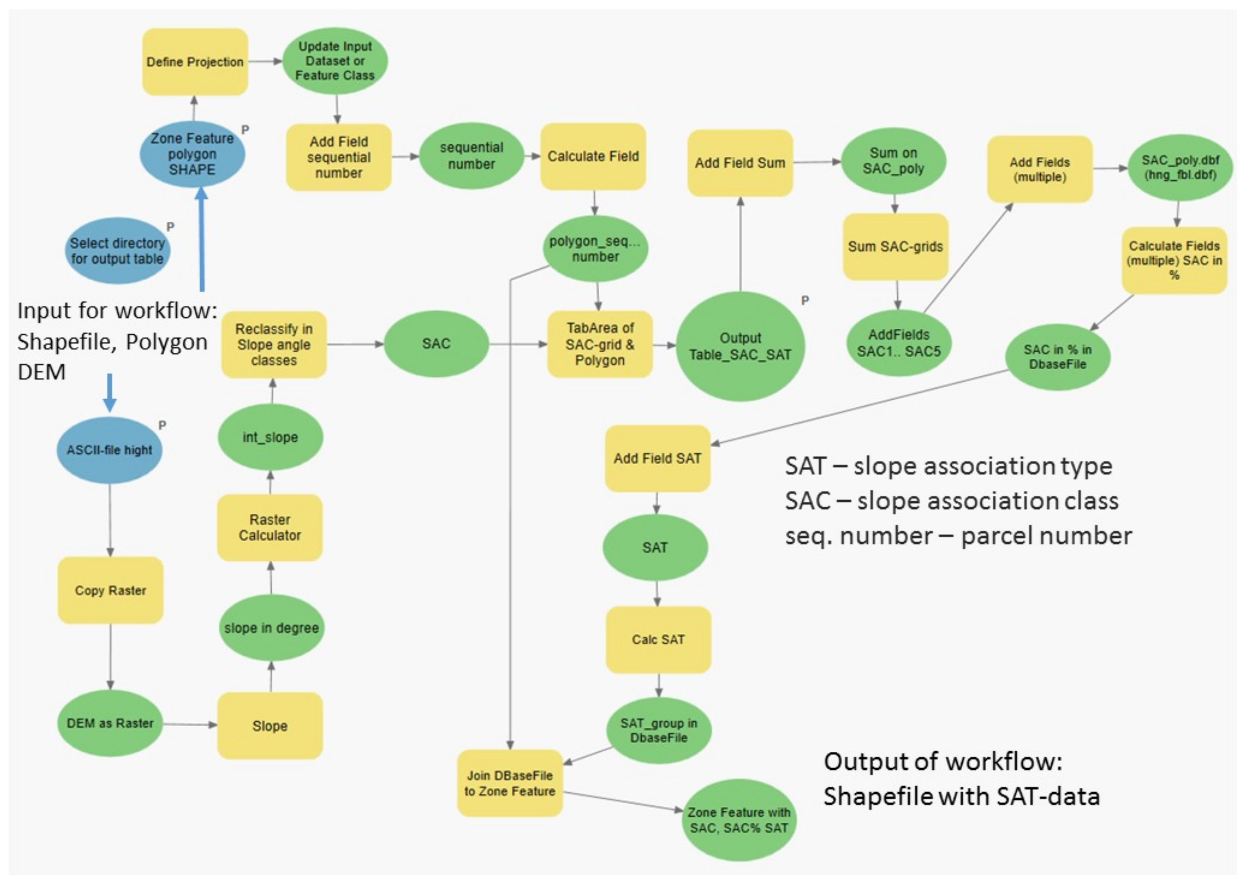
Using the geoprocessing tools of ArcGisPro 2.7, a workflow for deriving the SAT per reference area unit was elaborated in the model builder (Figure 1). The following main processing steps were implemented:
- Calculation of the slope’s inclination of the raster (DEM1 or DEM10);
- Reclassification of slope inclinations into SACs;
- Calculation of SAC’s units per reference area;
- Join resulting SAC units (SAC1–5 as area sum and area portion, SAT01–11 or numbered from 1 to 6, see Table 1) to the respective reference area (initial polygons);
- Thus, the combining assessment can be displayed on the map. With the identifier, the individual values from the table can be queried, or the table itself can be further processed for evaluation.
The algorithm developed with MMK to determine the SAT (Table 1) is also used in the present agricultural site survey [25,27].
The history of its development led to various verbal descriptions of the shorter form (Table 1 and Table 2) and longer form as well as to the more precise information required due to the use of GIS (Table 2), which are included in the following tables and legends of the figures.
The boundaries of the administrative units (NUTS3, county), the field blocks, and natural areas are available digitally. The boundaries of the catchment areas around wetlands, on the other hand, were calculated from the DEM. Previously, the information contained in ATKIS and in the field block cadastre on small standing waters and wetlands had to be merged since the LPIS partly contains more up-to-date data. For this purpose, all surface waters from ATKIS and the wetlands from field block cadastre were combined with “Merge” and their origin coded (ATKIS or LPIS). For all non-linear bodies of water, their catchment areas were then calculated. Within these catchment boundaries, the SATs were calculated according to Table 2 with the regulations by the Plant Protection Service and Figure 1. Thus, an SAT and the respective individual values of the areas and area shares of the slope angle classes (SAC) could be shown in the database for each catchment area of all water bodies in the regarded landscape unit (small lakes, ponds, wetland biotopes).
3. Results
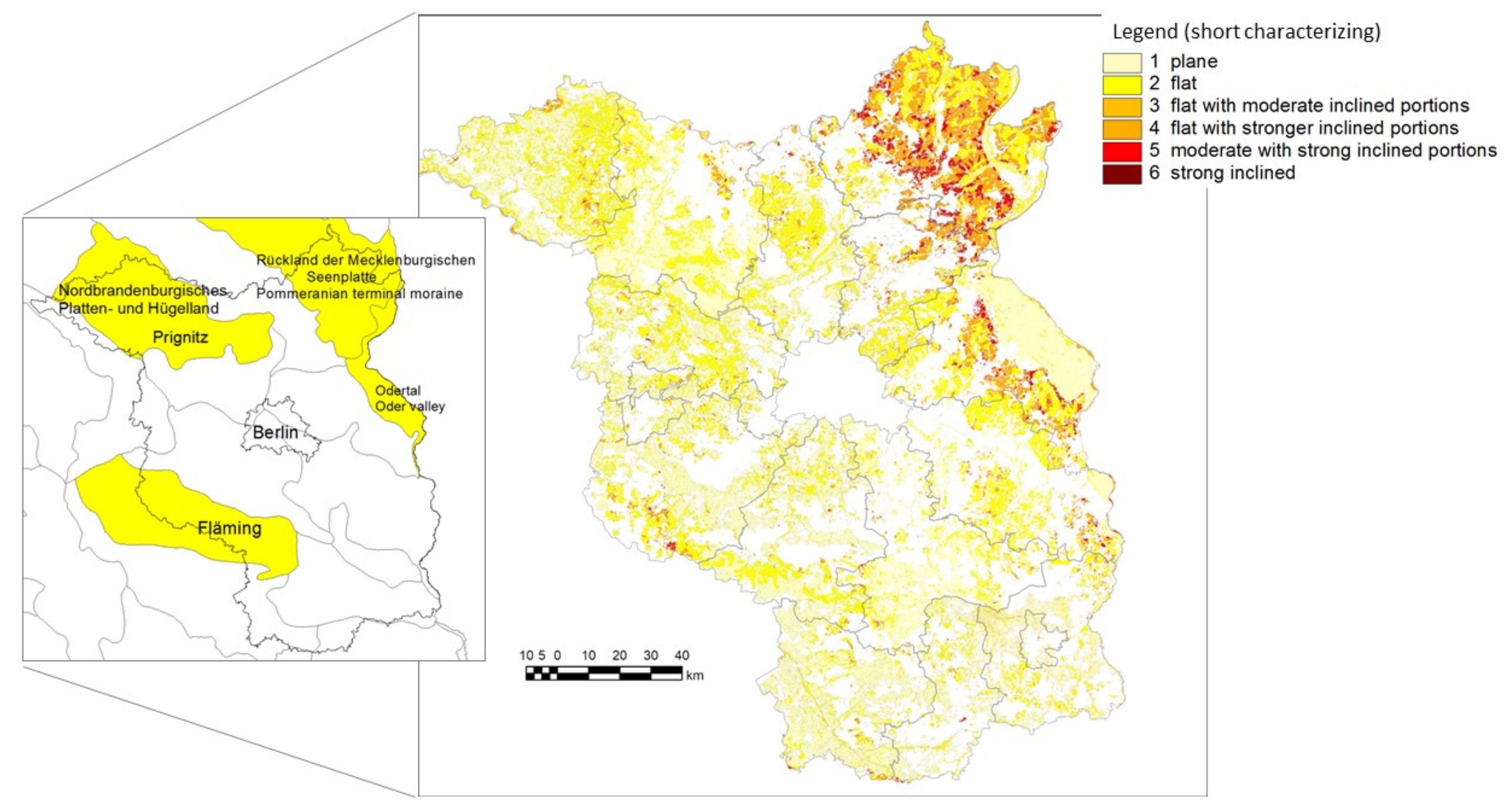
In the erosion risk maps of the EU, Brandenburg is shown as less vulnerable to erosion due to the lower relief energy [34]. The National Atlas of the Federal Republic of Germany also shows only low water erosion risks due to the scale, as the value range also includes mountainous regions [35]. However, the results of the DEM analysis also show larger areas with steeper slopes. The erosion problems of Brandenburg originate from the last and second-last glaciations, which left a variety of small-scale surface forms. The steeper slopes are mainly located in the domed-shaped ground moraine and terminal moraines in the Northeast of Brandenburg and the slopes of the Oder Valley in the east (Figure 2). More gentle, but longer slopes can be found in the heights of the Fläming in the southwest.
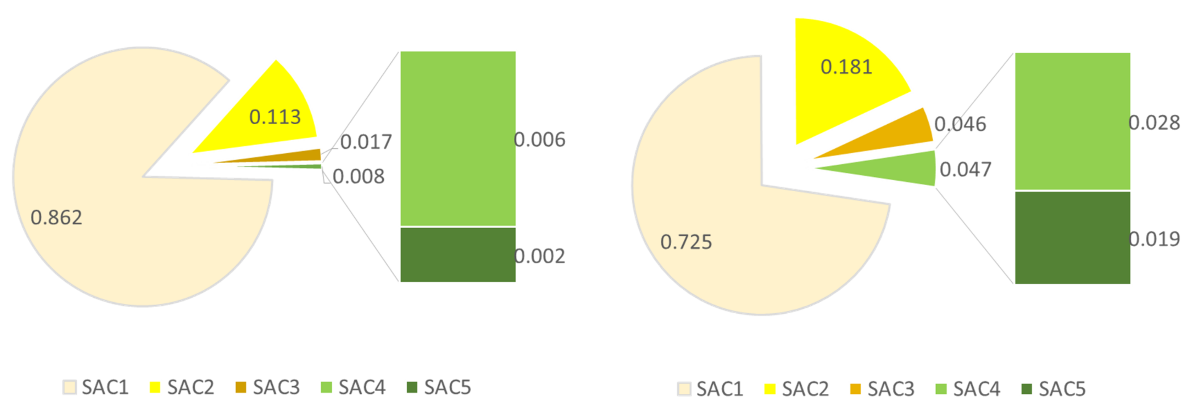
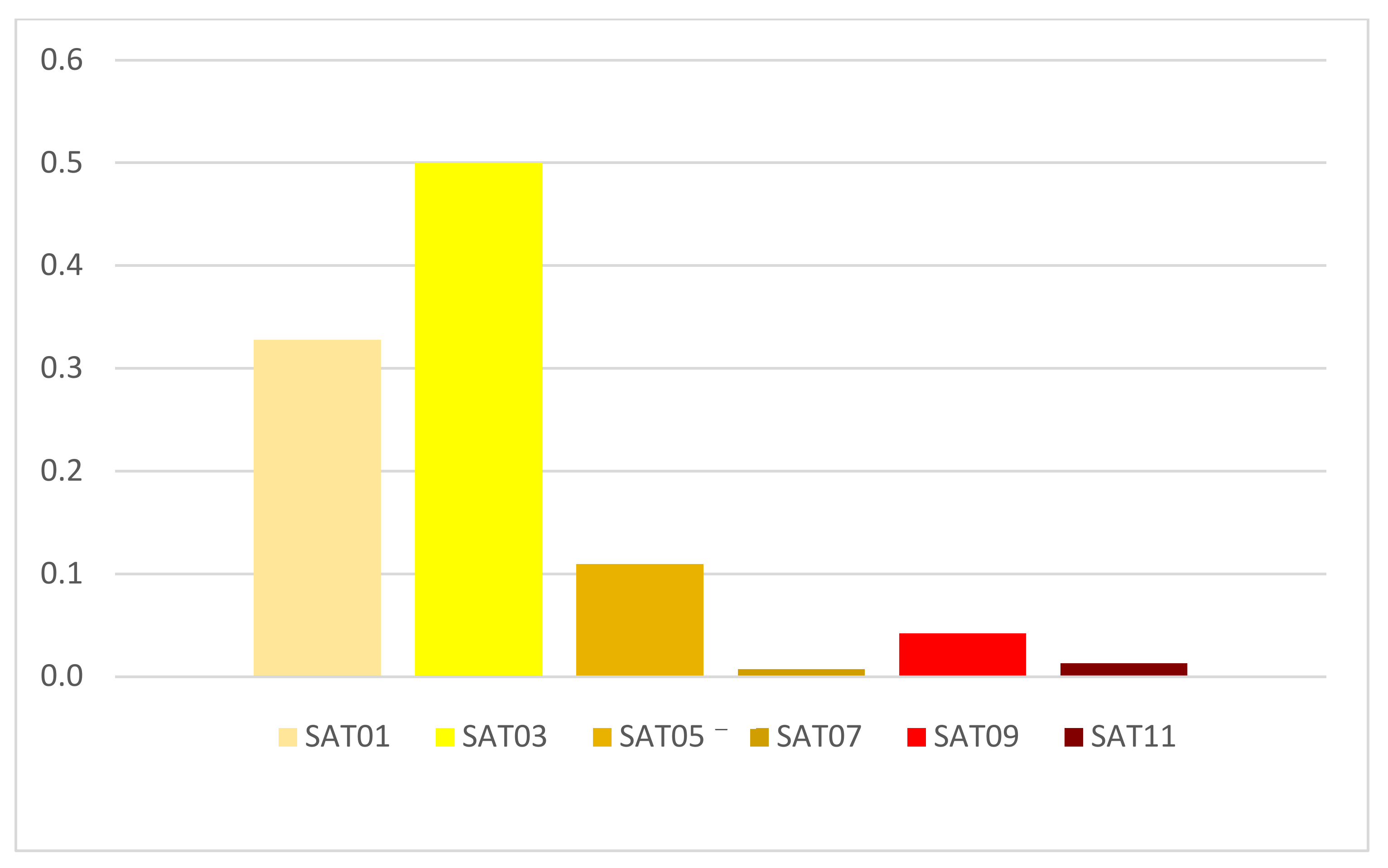
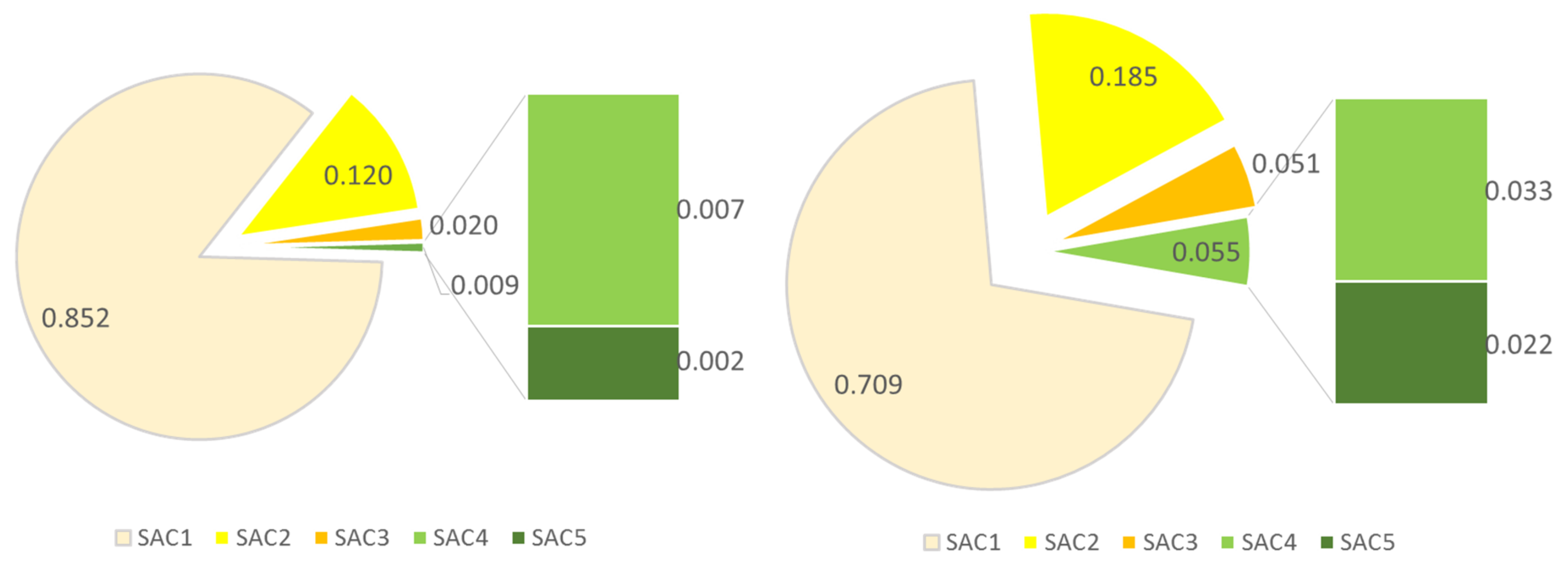
The suitability of the sloped surfaces for agricultural production is also reflected in the proportions of land use within the rural counties (Figure 3). The high proportion of forest in Brandenburg can be attributed to two factors: sandy soils with low fertility and steep slopes making management complicated. The affected area becomes clear when the percentages of each SAC are compared once to the total area of a county and once to the agriculturally used land area only. The share of agricultural land in Brandenburg varies greatly between the counties, with a minimum of about one-third (Barnim, Oberspreewald-Lausitz, Spree-Neiße) and a maximum of two-thirds (Prignitz). At the county level, SAC_5 is, on average, an order of magnitude larger. These higher proportions are correlated to land use as forest mainly there, whereas agriculture traditionally uses the more level sites (Table 3, Figure 4). Therefore, the shares of SAC_1 of agriculturally used land (Table 3, left part) are significantly larger than the shares of SAC_1 related to the total areas of the counties. The same is evident largely in the proportion of SAC of field blocks related to natural areas. The fertile plains are particularly heavily used for agriculture (Oder Valley, Table 4, Figure 5). Figure 4 compares the proportions of all six SATs of the field blocks in Brandenburg. This supports the statements made above.
The worldwide same reasons for the selection of agricultural land can be seen here at the federal state level: flat, fertile areas are used more intensively, before, due to the pressure of use, agriculture is increasingly carried out in unfavorable areas (see the work of [36,37], pp. 20–24 in the work of [38], and p. 224 in the work of [39]).
The example of selected field blocks in Brandenburg shows that smaller field blocks, in particular, have higher SAC (Table 5). Since field blocks are separated by natural and infrastructure boundaries (bodies of water, roads, paths), the field blocks with slopes are more often found in these classes. Since Brandenburg, as mentioned at the beginning, has relatively few sloping areas compared to the rest of Germany, large field blocks with primarily steep slopes are rare. In addition, this is also due to the fact that the heterogeneous topographical conditions are more averaged when referring to a larger area. Therefore, the SAT algorithm considers already higher SAC of proportions ≤5% (Table 1 and Table 2). The example data shown in Table 5 can also be categorized according to class boundaries of the area size, allowing determinations of rankings and orders for evaluations of environmental aspects as well as of the suitability for agricultural production of specific crops [40]. The comparison of the SAT of all field blocks in Brandenburg (Figure 4) shows again the predominant topography in Brandenburg: plane to flat with moderate inclined portions (SAT01–SAT05).
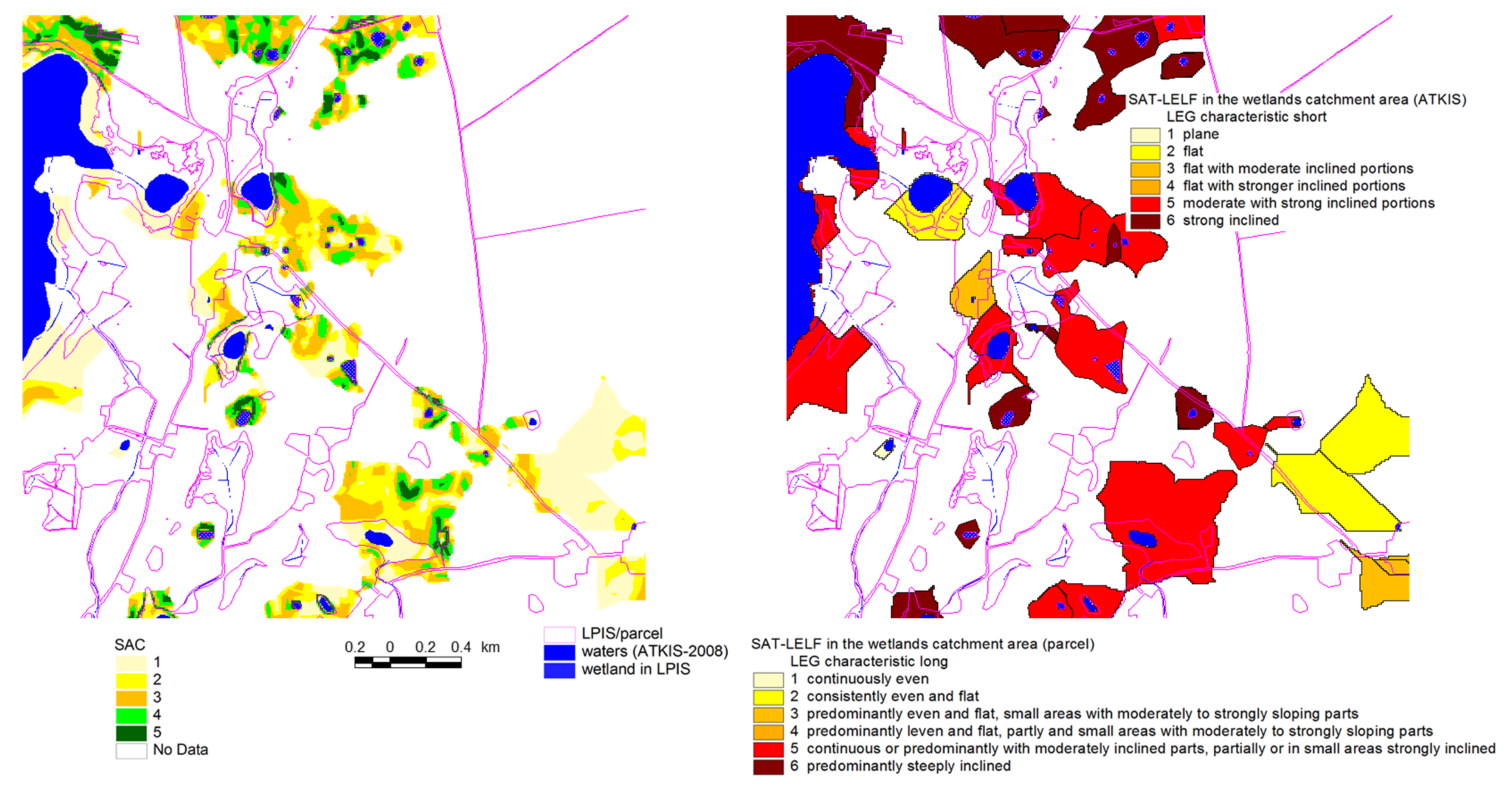
The protection of small water bodies and wetlands in agricultural used areas requires special precautions and restrictions. Fertilization and pest management have to take into account to prevent impacts to and damages of sensitive ecosystems [41]. In the case of possible matter transports by water erosion or runoff into small water bodies, it is necessary to identify all catchment areas and the contribution of slope angles inside them. Figure 6 shows an example in which the SAC (slope angle classes, on the left) and the resulting SAT (slope association type, on the right) were estimated using the algorithm of Table 2. Accordingly, the management can take into account the environmental concerns. This information is available for the farmers, administrations, and the general public on the Internet [42].
4. Discussion
Landscapes in northeastern Germany are characterized by a small-scale change of basic features. Nevertheless, the agricultural areas there are managed more or less uniformly. This results in the necessity of an integrative analysis within these management units. The SAT is a combining indicator to assess the topographic conditions within a regarded area unit, which is easy to apply and adapt. This allows conclusions about the influences of topography on environmental or technological limitations from a scientific point of view by summarizing without discretization. The SAT can thus serve as an indicator to justify environmental requirements in CAP or, as such, be used to justify direct payments. Further developments for the use of the SAT algorithms for cross-compliance rules instead of the assessment of erosion risk based on the erodibility of soil, slope inclination as well as rain erosivity currently used in Germany could be tested by combinations with curvature and exposure. An algorithm for estimating water erosion risk already exists by combining the SAT with the classified substrate association types (SFT) [17]. However, SFT’s does not exist for the entire Germany. They are also difficult to obtain from digital data on soil properties, compared to slope angles, which can be derived from the DEM easily. The soil properties in this form are not yet available nationwide on a high-resolution scale.
Besides the estimations of the SAT with a specific reference to an area, also integrative, whole-area analyses with the moving window method are possible [40]. With this method, the relief is reproduced, e.g., in reference radii of different widths, but with a categorizing result. The concerns still expressed by Thiere [43] that this approach is not free of subjectivity can be avoided by using GIS and automated procedures. Further, typing and classification have a cognitive effect. The SAT is suitable for many objectives, as soil and water protection, environmental protection or conservation, and promotion of biodiversity. So, the SAT can be helpful for decision support systems in environmental protection in general.
5. Conclusions
The SAT offers an alternative to expensive model calculations for initial assessments of local conditions for management decisions to derive suitability of regarded area units. Intended targets can include scientific, agro-technological, or environmental justified classes for the slopes. The final calculation includes SAT and the shares of the defined SAC for each area unit. Thus, there is ultimately one aggregated value for a variety of possible slopes within the area. This basic information on soil and water protection can be implemented with little effort and is traceable at any time. In combination with the association type of the substrate properties (SFT), basic site properties can be derived with little expenditure of time. If more precise assessments of material transport are necessary, the use of erosion models is essential.
Author Contributions
Conceptualization, methodology, software, validation, investigation, D.D. and L.V.; resources, D.D. and L.V.; writing—original draft preparation, D.D. and L.V.; writing—review and editing, D.D., T.K., and R.F.; visualization, D.D. and L.V.; project administration, D.D.; funding acquisition, D.D. All authors have read and agreed to the published version of the manuscript.
Funding
D.D., L.V., and R.F. were supported by the German Federal Ministry of Food and Agriculture (BMEL) and the Ministry for Science, Research and Culture of the State of Brandenburg (MWFK); T.K. was supported by the German Agency for Renewable Resources (FNR, 2220NR049B).
Institutional Review Board Statement
Not applicable.
Informed Consent Statement
Informed consent was obtained from all subjects involved in the study.
Data Availability Statement
Publicly available datasets were analyzed in this study. This data can be found in the references.
Acknowledgments
We thank the LGB and the Ministry of Agriculture, Environment and Climate Protection (MLUK) for providing DEM and InVeKoS-data, Horst H. Gerke (ZALF), and three unnamed reviewers for their helpful comments.
Conflicts of Interest
The authors declare no conflict of interest.
References
- European Soil Data Centre. European Soil Database Maps. Available online: https://esdac.jrc.ec.europa.eu/resource-type/european-soil-database-maps (accessed on 14 October 2021).
- Panagos, P.; Borrelli, P.; Meusburger, K. A New European Slope Length and Steepness Factor (LS-Factor) for Modeling Soil Erosion by Water. Geosciences 2015, 5, 117–126. [Google Scholar] [CrossRef] [Green Version]
- E.C. The Common Agricultural Policy at a Glance. Available online: https://ec.europa.eu/info/food-farming-fisheries/key-policies/common-agricultural-policy/cap-glance_en (accessed on 25 October 2021).
- Haase, G.; Hubrich, H.; Schlüter, H.; Mannsfeld, K.; Kugler, H.; Richter, H.; Barsch, H.; Kopp, D.; Schwanecke, W. Kennzeichnung und Kartierung von Naturraumtypen im mittleren Maßstabsbereich. Leipzig; Institut für Geographie und Geoökologie der AdW der DDR: Leipzig, Germany, 1982; p. 152. [Google Scholar]
- Gündra, H.; Assmann, A.; Jäger, S. Geomorphometrische Parameter mit hydrologischer Relevanz und die Qualität der zugrunde liegenden Digitalen Höhenmodelle. Hydrol. Wasserbewirtsch. 2000, 44, 114–121. [Google Scholar]
- Chifflard, P. Der Einfluss des Reliefs, der Hangsedimente und der Bodenvorfeuchte auf die Abflussbildung im Mittelgebirge—Experimentelle Prozess-Studien im Sauerland; Im Selbstverlag: Bochum, Germany, 2006; Volume Heft 76. [Google Scholar]
- Deumlich, D.; Schmidt, R.; Sommer, M. A multiscale soil–landform relationship in the glacial-drift area based on digital terrain analysis and soil attributes. J. Plant. Nutr. Soil Sci. 2010, 173, 843–851. [Google Scholar] [CrossRef]
- Kugler, H. Naturraumtypen des Ballungsraumes Leipzig Einschließlich Eines 1. Entwurfs zur Kennzeichnung des Reliefs im Rahmen der NK100; Martin-Luther-Univ: Halle, Germany, 1979; Manuscript 79/15. [Google Scholar]
- TGL. Aufnahme landwirtschaftlicher Standorte Georelief. In TGL 24300/03; TGL: Berlin, Germany, 1985; p. 6. [Google Scholar]
- Estler, M.; Pfahler, K. Einfluß der Hangneigung auf den Wert Landwirtschaftlicher Grundstücke; Bayerisches Staatsministerium für Ernährung, Landwirtschaft und Forsten: München, Germany, 1985; Volume Heft 8, p. 163. [Google Scholar]
- Ullrich, G.; Stengler, K.H. Arbeitssicherheit beim Einsatz von Traktoren und Landmaschinen im Hängigen Gelände; Verl. Tribuene: Berlin, Germany, 1971. [Google Scholar]
- Rothkegel, W. Landwirtschaftliche Schätzungslehre; Eugen Ulmer: Stuttgart, Germany, 1952. [Google Scholar]
- Greif, F. Raumstruktur-Inventar für das Österreichische Bundesgebiet. Eine Methodik zur Quantifizierung von Höhenlage, Hangneigung und Exposition; Agrarwirtschaftliches Institut des Bundesministeriums für Land- und Forstwirtschaft: Wien, Austria, 1980. [Google Scholar]
- ad-hoc-AG-Boden. Bodenkundliche Kartieranleitung. KA5; Schweizerbart’sche Verlagsbuchhandlung Stuttgart: Stuttgart, Germany, 2006; p. 468. [Google Scholar]
- Kasch, W.; Flegel, R. Landwirtschaftliche Bedeutung, Erfassung und Kennzeichnung der Reliefverhältnisse. Feldwirtschaft 1975, 1, 4. [Google Scholar]
- Diemann, R. Reliefsystematik auf der Grundlage der MMK. In Arch. Acker-u. Pflanzenbau u. Bodenkd; Akademie Verlag: Berlin, Germany, 1980; pp. 469–474. [Google Scholar]
- Schmidt, R.; Diemann, R.; Thiere, J.; Bickenbach, J.; Strohbach, B.; Succow, M.; Wünsche, M. Erläuterungen zur Mittelmaßstäbigen Landwirtschaftlichen Standortkartierun (MMK); Akademie Verlag: Eberswalde, Germany, 1981; p. 78. [Google Scholar]
- Reiher, W.; Grafe, B. Informationssystem Bodenführung ISBO—Anwenderhandbuch; Informationssystem Bodenführung: Markkleeberg, Germany, 1989; p. 95. [Google Scholar]
- Lieberoth, I.; Dunkelgod, P.; Gunia, W.; Thiere, J. Auswertungsrichtlinie MMK (Stand 1983); Akademieverlag: Berlin, Germany, 1983; p. 55. [Google Scholar]
- Klečka M. a kol. Bonitace čs. Zemědělských půd a Směry Jejich Využití. 1. díl, Vymezení a Mapování Bonitovaných Půdně–Ekologických Jednotek ČSSR. Uživatelská Příručka pro Užívání Map BPEJ; Federální Ministerstvo Zemědělství a Výživy: Praha-Bratislava, Slovakia, 1984; p. 131. [Google Scholar]
- Vitejte v eKatalogu BPE, JVÚMOP. Available online: https://bpej.vumop.cz/ (accessed on 25 October 2021).
- Koćmit, A.; Niedźwiecki, E.; Zabłocki, Z. Gleboznawstwo z Elementami Geologii; Wydawnictwo Akademii Rolniczej: Szczecin, Poland, 1990. [Google Scholar]
- Borrelli, P.; Alewell, C.; Alvarez, P.; Anache, J.A.A.; Baartman, J.; Ballabio, C.; Bezak, N.; Biddoccu, M.; Cerdà, A.; Chalise, D.; et al. Soil erosion modelling: A global review and statistical analysis. Sci. Total Environ. 2021, 780, 146494. [Google Scholar] [CrossRef] [PubMed]
- ESRI. ArcGIS Desktop: Release 10; Environmental Systems Research Institute: Redlands, CA, USA, 2011. [Google Scholar]
- Deumlich, D.; Dannowski, R.; Völker, L. Historische und aktuelle Geoinformation—Grundlage in der Agrarlandschaftsforschung. ZFV Z. Geodäsie Geoinf. Landmanag. 2014, 139, 329–341. [Google Scholar] [CrossRef]
- BfJ. Verordnung über die Anwendung von Düngemitteln, Bodenhilfsstoffen, Kultursubstraten und Pflanzenhilfsmitteln Nach den Grundsätzen der Guten Fachlichen Praxis Beim Düngen. 2017. Available online: https://www.gesetze-im-internet.de/d_v_2017/BJNR130510017.html (accessed on 14 October 2021).
- FAO. Guidelines for Soil Description; FAO: Rome, Italy, 2006. [Google Scholar]
- LGB. Digitales Geländemodell (DGM). Available online: https://geobroker.geobasis-bb.de/gbss.php?MODE=GetProductInformation&PRODUCTID=488a2b53-564f-43eb-88ec-0d87bb43ed20 (accessed on 14 October 2021).
- Katzur, L.; Schönitz, A.; Wedel, H. Digitale Höhen für jeden Quadratmeter Brandenburgs; Vermessung Brandenburg, MdI Brandenburg: Potsdam, Germany, 2013; p. 8. [Google Scholar]
- InVeKoS-DZ. Digitales Feldblock Kataster; Landesvermessung und Geobasisinformation Brandenburg (LGB): Potsdam, Germany, 2020. [Google Scholar]
- Meynen, E.; Schmithüsen, J. Handbuch der naturräumlichen Gliederung Deutschlands/unter Mitwirkung des Zentralausschusses für Deutsche Landeskunde, 1953–1962; Bundesanst für Landeskunde u. Raumforschung: Bad Godesberg, Germany, 1962; p. 608S. [Google Scholar]
- EUROSTAT. NUTS—Nomenclature of Territorial Units for Statistics. Available online: https://ec.europa.eu/eurostat/web/nuts/background (accessed on 14 October 2021).
- ESRI. What Is ModelBuilder? ESRI: West Redlands, CA, USA; Available online: https://pro.arcgis.com/de/pro-app/latest/help/analysis/geoprocessing/modelbuilder/what-is-modelbuilder-.htm (accessed on 20 November 2021).
- Panagos, P.; Pasquale, B.; Jean, P.; Cristiano, B.; Emanuele, L.; Katrin, M.; Luca, M.; Christine, A. The new assessment of soil loss by water erosion in Europe. Environ. Sci. Policy 2015, 54, 438–447. [Google Scholar] [CrossRef]
- Fohrer, N.; Mollenhauer, K.S.; Thomas, B. Nationalatlas Bundesrepublik Deutschland; Liedtke, H.M., Roland, S., Karl, H., Eds.; Spektrum Akad. Verl.: Heidelberg/Berlin, Germany, 2003; Volume 2, p. 173. [Google Scholar]
- Nitsch, H.; Osterburg, B.; Roggendorf, W. Landwirtschaftliche Flächennutzung im Wandel–Folgen für Natur und Landschaft; NABU-Bundesverband & Deutscher Verband für Landschaftspflege (DVL) e.V.: Berlin, Germany, 2009; p. 39. [Google Scholar]
- Küster, H. Geschichte der Landschaft in Mitteleuropa: Von der Eiszeit bis zur Gegenwart; Beck: München, Germany, 1996. [Google Scholar]
- Krenzlin, A. Dorf, Feld und Wirtschaft im Gebiet der großen Täler und Platten östlich der Elbe: Eine Siedlungsgeographische Untersuchung; Verl. d. Amtes f. Landeskunde: Remagen, Germany, 1952; p. 144. [Google Scholar]
- Bork, H.R.; Bork, H.; Dalchow, C.; Faust, B.; Piorr, H.-P.; Schatz, T. Landschaftsentwicklung in Mitteleuropa; Klett-Perthes: Gotha, Germany; Stuttgart, Germany, 1998. [Google Scholar]
- Deumlich, D.; Kiesel, J.; Thiere, J.; Reuter, H.-I.; Völker, L.; Funk, R. Application of the SIte COmparison Method (SICOM) to assess the potential erosion risk—A basis for the evaluation of spatial equivalence of agri-environmental measures. Catena 2006, 68, 141–152. [Google Scholar] [CrossRef]
- Ministerium für Landwirtschaft. Mluk. Cross Compliance 2021; Umwelt und Klimaschutz des Landes Brandenburg: Potsdam, Germany, 2020; p. 115. [Google Scholar]
- MLUK. Digitales Feldblockkataster GIS InVeKoS. Available online: https://maps.brandenburg.de/WebOffice/?project=DFBK_www_CORE (accessed on 15 November 2021).
- Thiere, J. Zu einigen Problemen der Entwicklung und Systematik landwirtschaftlich genutzter Böden. Wiss. Zschr. Humboldt-Univ. Berlin Math.-Nat. R. 1972, XXl, 288–296. [Google Scholar]
Figure 1.
Flow chart to calculate slope association types (SAT) with the ModelBuilder of ArcGISPro 2.7 [33].
Figure 1.
Flow chart to calculate slope association types (SAT) with the ModelBuilder of ArcGISPro 2.7 [33].

Figure 2.
Slope association type of parcels in Brandenburg based on DEM1 with NUTS3 borderlines; © GeoBasis-DE/LGB (2020), https://www.govdata.de/dl-de/by-2-0 (accessed on 14 October 2021).
Figure 2.
Slope association type of parcels in Brandenburg based on DEM1 with NUTS3 borderlines; © GeoBasis-DE/LGB (2020), https://www.govdata.de/dl-de/by-2-0 (accessed on 14 October 2021).

Figure 3.
Distribution of slope angle classes of all parcels (left) and counties (right).

Figure 4.
Slope association type—portion of parcels (n~92,000) in Brandenburg, same color scheme as in Table 2.
Figure 4.
Slope association type—portion of parcels (n~92,000) in Brandenburg, same color scheme as in Table 2.

Figure 5.
Distribution of slope angle classes of all parcels (left) and natural areas (right).

Figure 6.
Slope angle classes (SAC) and slope association types (SAT) in the catchments of water bodies inside field blocks, based on the work of [28], same color scheme as in Table 2.


Table 1.
Original slope association types of the medium-scale agricultural site mapping [17], p. 15.
Table 1.
Original slope association types of the medium-scale agricultural site mapping [17], p. 15.
| Original Criterion to Estimate the Slope Association Type (SAT) | |||||||
|---|---|---|---|---|---|---|---|
| Slope Association Type | Summarized Slope Angle Classes (SSAC I–V) | ||||||
| Slope Angle Classes (SAC 0–8) | |||||||
| Symbol | No. | Description | I | II | III | IV | V |
| 0 | 1 | 2/3 | 4/5 | 6–8 | |||
| <4% | 4–9% | 9–14% | 14–23% | >23% | |||
| 01 | 0 | Plane | ≥95 | ≤5 | 0 | ||
| 03 | 1 | Flat | ≥60–80 | ≤40 | ≤5 | 0 | |
| 05 | 2 | Flat with moderate inclined portions | ≥80 | ≤20 | ≤5 | 0 | |
| 07 | 3 | Flat with strong inclined portions | ≥80 | ≤20 | ≤5 | ||
| 09 | 4 | Moderate with strong inclined portions | ≥40–60 | ≥20–40 | ≤20 | ≤5 | |
| 11 | 5 | Strong inclined | ≥40–60 | ≥40–60 | |||
Table 2.
Criterion to estimate the slope association type (specified [25]) adopted from Schmidt et al., 1981 [17].
| Slope Association Type (SAT) | Combined Slope Angle Classes (SAC) 1 Slope Angle Criterion 2,3 | |||||
|---|---|---|---|---|---|---|
| 1 | 2 | 3 | 4 | 5 | ||
| Symbol 4 Nr/SAT | Description | ≤4% 2 ≤2%3 | 4%–≤9% 2%–≤4% | 9%–≤14% 4%–≤8% | 14%–≤23% 8%–≤13% | >23% >13% |
| 1/01 | Plane | ≥95 | ≤5 | 0 | ||
| 2/03 | Flat | ≥60 | ≤40 | 0 | ||
| 3/05 | Flat with moderate inclined portions | ≥80 | ≤20 | ≤5 | 0 | |
| 4/07 | Flat with stronger inclined portions | ≥80 | ≤20 | ≤5 | ||
| 5/09 | Moderate with strong inclined portions | ≥70 | <30 | |||
| 6/11 | Strong inclined | <70 | ≥30 | |||
Table 3.
Shares of SAC in relation to the area of agricultural used land LPIS (AF) and to the total area of the county.
Table 3.
Shares of SAC in relation to the area of agricultural used land LPIS (AF) and to the total area of the county.
| Area Share of LPIS | Area Share of County Area | ||||||||||
|---|---|---|---|---|---|---|---|---|---|---|---|
| County Name | SAC1 | SAC2 | SAC3 | SAC4 | SAC5 | Share of AF | SAC1 | SAC2 | SAC3 | SAC4 | SAC5 |
| Barnim | 0.749 | 0.195 | 0.038 | 0.015 | 0.004 | 0.330 | 0.611 | 0.236 | 0.074 | 0.049 | 0.030 |
| Dahme-Spreewald | 0.910 | 0.076 | 0.009 | 0.003 | 0.001 | 0.353 | 0.744 | 0.173 | 0.045 | 0.025 | 0.013 |
| Elbe-Elster | 0.943 | 0.046 | 0.006 | 0.003 | 0.002 | 0.484 | 0.802 | 0.140 | 0.028 | 0.017 | 0.013 |
| Havelland and Potsdam | 0.915 | 0.075 | 0.007 | 0.002 | 0.001 | 0.506 | 0.761 | 0.158 | 0.040 | 0.025 | 0.015 |
| Märkisch-Oderland | 0.811 | 0.147 | 0.029 | 0.010 | 0.003 | 0.581 | 0.678 | 0.193 | 0.058 | 0.038 | 0.033 |
| Oberhavel | 0.877 | 0.104 | 0.012 | 0.005 | 0.002 | 0.394 | 0.731 | 0.177 | 0.046 | 0.029 | 0.016 |
| Oder-Spree and Frankfurt/O. | 0.805 | 0.167 | 0.020 | 0.006 | 0.002 | 0.346 | 0.679 | 0.204 | 0.056 | 0.036 | 0.024 |
| Oberspreewald-Lausitz | 0.932 | 0.058 | 0.006 | 0.003 | 0.001 | 0.300 | 0.759 | 0.160 | 0.034 | 0.024 | 0.023 |
| Ostprignitz | 0.903 | 0.085 | 0.008 | 0.003 | 0.001 | 0.512 | 0.784 | 0.152 | 0.033 | 0.019 | 0.012 |
| Prignitz | 0.904 | 0.082 | 0.008 | 0.004 | 0.003 | 0.646 | 0.802 | 0.143 | 0.028 | 0.016 | 0.011 |
| Potsdam-Mittelmark and Brandenburg | 0.891 | 0.097 | 0.009 | 0.002 | 0.000 | 0.396 | 0.732 | 0.189 | 0.042 | 0.023 | 0.014 |
| Spree-Neiße and Cottbus | 0.920 | 0.068 | 0.007 | 0.003 | 0.002 | 0.319 | 0.751 | 0.160 | 0.036 | 0.025 | 0.028 |
| Teltow-Fläming | 0.925 | 0.067 | 0.005 | 0.002 | 0.001 | 0.431 | 0.764 | 0.165 | 0.037 | 0.021 | 0.013 |
| Uckermark | 0.585 | 0.313 | 0.074 | 0.025 | 0.004 | 0.575 | 0.558 | 0.289 | 0.086 | 0.045 | 0.022 |
Table 4.
Area portion of SAC in LPIS and natural areas; AF-agricultural used area: area portion relative to the natural area [31,35].
| Natural Area | Aggregated on LPIS (Parcel Sum) | AF Rel. | Aggregated on Natural Area [31] | ||||||||||
|---|---|---|---|---|---|---|---|---|---|---|---|---|---|
| SAC1 | SAC2 | SAC3 | SAC4 | SAC5 | km2 | (LPIS) | SAC1 | SAC2 | SAC3 | SAC4 | SAC5 | km2 | |
| Sächsisches Hügelland (einschl. Leipziger Land) | 0.618 | 0.320 | 0.051 | 0.010 | 0.001 | 7.07 | 0.443 | 0.489 | 0.320 | 0.090 | 0.051 | 0.050 | 15.96 |
| Rückland der Mecklenburgischen Seenplatte | 0.557 | 0.333 | 0.080 | 0.026 | 0.004 | 1659.09 | 0.649 | 0.526 | 0.308 | 0.094 | 0.049 | 0.022 | 2555.74 |
| Mecklenburgische Seenplatte | 0.714 | 0.225 | 0.044 | 0.014 | 0.003 | 373.38 | 0.202 | 0.598 | 0.247 | 0.080 | 0.050 | 0.025 | 1849.31 |
| Südwestliches Vorland der Mecklenburgischen Seenplatte | 0.937 | 0.050 | 0.008 | 0.004 | 0.001 | 0.39 | 0.358 | 0.593 | 0.184 | 0.106 | 0.083 | 0.034 | 1.08 |
| Nordbrandenburgisches Platten-und Hügelland | 0.894 | 0.094 | 0.008 | 0.003 | 0.001 | 2342.95 | 0.572 | 0.790 | 0.155 | 0.029 | 0.016 | 0.010 | 4096.68 |
| Luchland | 0.930 | 0.060 | 0.006 | 0.003 | 0.001 | 1211.66 | 0.571 | 0.805 | 0.131 | 0.031 | 0.020 | 0.012 | 2121.71 |
| Ostbrandenburgische Platte | 0.746 | 0.207 | 0.033 | 0.011 | 0.003 | 1204.92 | 0.480 | 0.622 | 0.238 | 0.066 | 0.042 | 0.032 | 2508.42 |
| Odertal (Oder valley) | 0.918 | 0.056 | 0.013 | 0.008 | 0.005 | 720.37 | 0.655 | 0.805 | 0.111 | 0.032 | 0.025 | 0.027 | 1099.06 |
| Mittelbrandenburgische Platten und Niederungen | 0.922 | 0.069 | 0.007 | 0.002 | 0.001 | 1547.29 | 0.430 | 0.770 | 0.153 | 0.038 | 0.024 | 0.015 | 3598.37 |
| Ostbrandenburgisches Heide-und Seengebiet | 0.838 | 0.136 | 0.018 | 0.006 | 0.002 | 1007.88 | 0.266 | 0.683 | 0.203 | 0.058 | 0.035 | 0.022 | 3784.48 |
| Spreewald | 0.955 | 0.036 | 0.005 | 0.003 | 0.001 | 411.02 | 0.447 | 0.817 | 0.117 | 0.029 | 0.020 | 0.017 | 918.64 |
| Lausitzer Becken und Heideland | 0.930 | 0.062 | 0.005 | 0.002 | 0.001 | 982.85 | 0.355 | 0.764 | 0.162 | 0.032 | 0.021 | 0.021 | 2768.81 |
| Fläming | 0.882 | 0.106 | 0.009 | 0.002 | 0.000 | 1007.88 | 0.427 | 0.715 | 0.211 | 0.042 | 0.021 | 0.011 | 2358.70 |
| Elbtalniederung | 0.919 | 0.062 | 0.009 | 0.005 | 0.005 | 457.15 | 0.445 | 0.787 | 0.140 | 0.036 | 0.023 | 0.014 | 1026.56 |
| Elbe-Mulde-Tiefland | 0.947 | 0.042 | 0.005 | 0.003 | 0.002 | 621.48 | 0.595 | 0.828 | 0.117 | 0.025 | 0.017 | 0.013 | 1045.13 |
| Oberlausitzer Heideland | 0.919 | 0.057 | 0.012 | 0.008 | 0.004 | 65.46 | 0.178 | 0.748 | 0.164 | 0.034 | 0.025 | 0.028 | 367.57 |
Table 5.
Example of data sets of estimated slope association types; parcel is anonymized.
| GIS-ID | SAC1 | SAC2 | SAC3 | SAC4 | SAC5 | sum | SAC1_rel | SAC2_rel | SAC3_rel | SAC4_rel | SAC5_rel | SAT | Area |
|---|---|---|---|---|---|---|---|---|---|---|---|---|---|
| No. | m2 | % | ha | ||||||||||
| 4069 | 341,644 | 128,424 | 106,752 | 152,844 | 138,196 | 867,860 | 39.37 | 14.80 | 12.30 | 17.61 | 15.92 | 6 | 86.8 |
| 1798 | 324,216 | 383,368 | 95,000 | 11,252 | 56 | 813,892 | 39.84 | 47.10 | 11.67 | 1.38 | 0.01 | 3 | 81.4 |
| 5410 | 239,832 | 256,768 | 99,728 | 26,924 | 948 | 624,200 | 38.42 | 41.14 | 15.98 | 4.31 | 0.15 | 5 | 62.4 |
| 4345 | 229,672 | 223,772 | 89,856 | 41,980 | 5740 | 591,020 | 38.86 | 37.86 | 15.20 | 7.10 | 0.97 | 5 | 59.1 |
| 4139 | 350,444 | 82,296 | 47,248 | 26,980 | 1600 | 508,568 | 68.91 | 16.18 | 9.29 | 5.31 | 0.31 | 4 | 50.9 |
| 4520 | 195,612 | 257,496 | 48,488 | 6488 | 24 | 508,108 | 38.50 | 50.68 | 9.54 | 1.28 | 0.00 | 3 | 50.8 |
| 2992 | 213,056 | 241,080 | 43,160 | 11,264 | 68 | 508,628 | 41.89 | 47.40 | 8.49 | 2.21 | 0.01 | 3 | 50.9 |
| 5247 | 230,720 | 122,000 | 72,528 | 54,356 | 7992 | 487,596 | 47.32 | 25.02 | 14.87 | 11.15 | 1.64 | 5 | 48.8 |
| 4782 | 183,368 | 171,640 | 56,432 | 22,984 | 3500 | 437,924 | 41.87 | 39.19 | 12.89 | 5.25 | 0.80 | 4 | 43.8 |
| 500 | 221,056 | 121,364 | 46,264 | 31,736 | 10,776 | 431,196 | 51.27 | 28.15 | 10.73 | 7.36 | 2.50 | 5 | 43.1 |
| 1950 | 399,064 | 27,672 | 1728 | 388 | 96 | 428,948 | 93.03 | 6.45 | 0.40 | 0.09 | 0.02 | 2 | 42.9 |
| 2938 | 414,236 | 7964 | 1688 | 1280 | 708 | 425,876 | 97.27 | 1.87 | 0.40 | 0.30 | 0.17 | 1 | 42.6 |
| 3850 | 314,416 | 105,744 | 4340 | 468 | 696 | 425,664 | 73.86 | 24.84 | 1.02 | 0.11 | 0.16 | 2 | 42.6 |
| 4824 | 421,672 | 3712 | 132 | 16 | 8 | 425,540 | 99.09 | 0.87 | 0.03 | 0.00 | 0.00 | 1 | 42.6 |
| 728 | 36,236 | 100,296 | 47,544 | 6820 | 20 | 190,916 | 18.98 | 52.53 | 24.90 | 3.57 | 0.01 | 5 | 19.1 |
| 4343 | 36,744 | 48,060 | 30,164 | 40,336 | 12,112 | 167,416 | 21.95 | 28.71 | 18.02 | 24.09 | 7.23 | 6 | 16.7 |
| 2272 | 6836 | 24,872 | 42,140 | 64,120 | 28,012 | 165,980 | 4.12 | 14.98 | 25.39 | 38.63 | 16.88 | 6 | 16.6 |
| 2483 | 36,304 | 80,816 | 24,740 | 6920 | 92 | 148,872 | 24.39 | 54.29 | 16.62 | 4.65 | 0.06 | 5 | 14.9 |
| 1667 | 17,448 | 34,124 | 33,612 | 38,436 | 23,872 | 147,492 | 11.83 | 23.14 | 22.79 | 26.06 | 16.19 | 6 | 14.7 |
| 2379 | 31,800 | 20,868 | 8824 | 12,624 | 5328 | 79,444 | 40.03 | 26.27 | 11.11 | 15.89 | 6.71 | 5 | 7.9 |
| 4788 | 34,800 | 17,976 | 7108 | 2492 | 640 | 63,016 | 55.22 | 28.53 | 11.28 | 3.95 | 1.02 | 3 | 6.3 |
| 2130 | 62,172 | 2136 | 124 | 0 | 0 | 64,432 | 96.49 | 3.32 | 0.19 | 0.00 | 0.00 | 1 | 6.4 |
Publisher’s Note: MDPI stays neutral with regard to jurisdictional claims in published maps and institutional affiliations. |
© 2021 by the authors. Licensee MDPI, Basel, Switzerland. This article is an open access article distributed under the terms and conditions of the Creative Commons Attribution (CC BY) license (https://creativecommons.org/licenses/by/4.0/).
Share and Cite
MDPI and ACS Style
Deumlich, D.; Völker, L.; Funk, R.; Koch, T. The Slope Association Type as a Comparative Index for the Evaluation of Environmental Risks. Water 2021, 13, 3333. https://0-doi-org.brum.beds.ac.uk/10.3390/w13233333
AMA Style
Deumlich D, Völker L, Funk R, Koch T. The Slope Association Type as a Comparative Index for the Evaluation of Environmental Risks. Water. 2021; 13(23):3333. https://0-doi-org.brum.beds.ac.uk/10.3390/w13233333
Chicago/Turabian StyleDeumlich, Detlef, Lidia Völker, Roger Funk, and Tobias Koch. 2021. "The Slope Association Type as a Comparative Index for the Evaluation of Environmental Risks" Water 13, no. 23: 3333. https://0-doi-org.brum.beds.ac.uk/10.3390/w13233333
Note that from the first issue of 2016, this journal uses article numbers instead of page numbers. See further details here.