Article

Diatoms from the Spring Ecosystems Selected for the Long-Term Monitoring of Climate-Change Effects in the Berchtesgaden National Park (Germany)

1
MUSE—Museo delle Scienze, Research & Collections Department (Limnology & Phycology), Corso del Lavoro e della Scienza 3, 38123 Trento, Italy
2
Department of Biological, Geological and Environmental Sciences—BiGeA, Alma Mater Studiorum University of Bologna, Via Irnerio 42, 40126 Bologna, Italy
3
Institute of Hydrobiology of NAS of Ukraine, Geroiv Stalingrada 12, 04210 Kyiv, Ukraine
4
Emilia-Romagna Region, Geological, Seismic & Soil Survey, Viale della Fiera, 8, 40127 Bologna, Italy
5
Klima-Zentrum, Bayerisches Landesamt für Umwelt, Hans-Högn-Straße 12, 95030 Hof/Saale, Germany
6
Department of Evolution and Ecology, Eberhard-Karls-Universität Tübingen, Auf der Morgenstelle 28E, 72076 Tübingen, Germany
7
Botany Department, Faculty of Science, Ain Shams University, Abbassia Square, Cairo 11566, Egypt
*
Author to whom correspondence should be addressed.
Submission received: 31 December 2021 / Revised: 23 January 2022 / Accepted: 24 January 2022 / Published: 27 January 2022

Abstract

:
We studied diatoms from the fifteen springs selected in the Berchtesgaden National Park on behalf of the Bavarian State Ministry for the Environment to be sentinel environments of climate-change effects. For three of these springs, diatom data based on samples taken in 1997 were also available. A total of 162 species belonging to 49 genera were found sampling three microhabitat types (lithic materials, bryophytes, surface sediments). The cumulative percentage of all species included in a threat category including endangered species was 43%, confirming previous findings for comparable environments of the Alps. We could find a statistically significant positive association between the Meinzer variability index for discharge and the cumulative relative abundance of aerial diatom species. This study thus highlighted once again the relevance of discharge (and associated water-level) variability as an environmental determinant of diatom assemblages in spring ecosystems. Increased nitrate concentrations in some springs, likely due to diffuse airborne pollution and, locally, to impacts such as forest management, game, and cattle, led to a relevant occurrence of eutraphentic diatom species. Our results show a segregation of the older data in non-parametric diatom-based ordinations, suggesting a strong potential for the use of spring diatoms in studies aiming at tracking the effects of climate and environmental change.

1. Introduction

Diatoms are a group of unicellular microalgae characterised by a silica frustule—with a structure often compared to a pillbox—that encloses the cell. Diatoms are very diverse and numerous microorganisms, with an estimated 100,000 species and infraspecies, and at least 30,000 currently extant taxa [1]. Ecologically, diatoms are common in fresh, brackish, and salty waters, and also in all terrestrial habitats where some moisture is at least sporadically available. Diatoms have a major role among the primary producers in the biosphere—about one-fifth of the net oxygen available in the atmosphere is consistently produced by diatoms (abundant also in the plankton of the oceans) [2]. Many diatom species have been documented to have very specific environmental preferences, and consequently, diatom ecology has been rigorously investigated [3].
A notable diatom-taxa richness is typically found in oligotrophic freshwater systems (e.g., [4]). Notwithstanding the special role of these systems for biodiversity conservation, revealed, for instance, by high numbers of rare and endangered Red-List taxa [5,6] and the relevant occurrence of endemic diatom taxa in the most isolated ones [7], diatoms in oligotrophic aquatic environments have been less-intensively studied than those in more impacted fresh waters [8]. However, oligotrophic aquatic habitats, such as headwaters, if in-depth studied, may provide important evidence for the identification of pristine/reference sites to inform conservation and restoration efforts. The aforementioned reasons have sometimes resulted in the inclusion of such aquatic systems in nature preserves. In spite of that, these kinds of habitats are becoming increasingly rare due to direct and indirect human impacts.
Headwater streams should be key elements in the building of protected-area networks, are characterised by close terrestrial-aquatic linkage, are very sensitive to natural or anthropogenic disturbance of the surrounding lands, are critical habitat for rare and endangered freshwater species, and in addition, they can play a significant role in the protection of riverine species during critical and specific periods of the year [9].
Springs, which are the source of many headwater streams, are probably the most representative oligotrophic aquatic habitats. They have unique qualities, such as a high degree of environmental organisation (differentiated conditions as regards e.g., ecomorphology, lithology, isolation, shading, the permanence of flow, current velocity, etc.) that provides a high heterogeneity, a multiple ecotone nature (groundwater—surface water, aquatic—terrestrial, spring mouth—running water system), a pronounced microhabitat-mosaic structure, and the opportunity to be a kind of shelter for the most sensitive species in densely populated and highly exploited areas [5].
Diatoms are excellent indicators for many reasons, the main ones being the high species diversity in almost any aquatic habitat and the distinct and thus informative ecological preferences of many species. Diatoms can, thus be successfully used as indicators in spring habitats with manifold applications [10]:
-
Value for nature conservation. Cantonati et al. [11] highlighted the potential of Diatom Red Lists [6,12] which allow a characterisation of the ecological integrity and of the diatom diversity of inland water ecosystems (also of practical importance to designate the most relevant habitats for conservation purposes), including a clear assessment of the threat status of the habitat. Furthermore, they offer ample possibilities to track the effects of stressors and of environmental change. The cumulative proportion of diatom species belonging to threat categories is a good indicator of spring-habitat ecological integrity as it consistently decreases with changes such as the increase in groundwater nitrates or spring-morphology alteration [5,11]. By comparison with an extensive stream-diatom database, we could recently show [13] that, in densely populated and exploited areas, springs are the last high integrity refugium for Red-List and sensitive (oligotraphentic) diatom species (Least-Impaired Habitat Relicts concept—LIHRe, [5]).
-
Water quality, including factors and parameters that are particularly relevant in springs (e.g., nitrates, often used as proxies of aquifer contamination in spring studies).
-
Contamination by metals and trace elements. Cantonati et al. [14] showed peculiar valve deformities of the widespread species Achnanthidium minutissimum (Kütz.) Czarn. could be used as indicators of copper, zinc, and antimony natural or anthropogenic contamination.
-
Spring classification. Spring types can be straightforwardly identified using diatoms [10] as many species respond with high sensitivity to the main parameters used in most spring classifications (current velocity, mineral content, substrata, light conditions, etc.).
-
Flow variability. Diatoms live not only in the wetted perimeter of springs, but also in microhabitats that are only periodically (discharge fluctuations) or intermittently (spray zones) provided with water. Thus, the composition of diatom assemblages can provide information on hydroperiod and flow variability and persistence (e.g., [10]), which is very useful in particular in explorative hydrogeological studies.
-
Springs-dependent species. Though no diatom species found exclusively in springs have been identified, there are species that occur mainly in the spring-fed headwaters of carbonate streams [15], and can thus even be used as indicators of “spring conditions” as opposed to “stream conditions”.
-
Geological substratum. The distribution of some diatom species is influenced by the geological substratum of the aquifer feeding the spring. Achnanthidium dolomiticum Cantonati et Lange-Bert. [16], for instance, is found in springs (and other aquatic habitats) with drainage basins formed by rocks that confer to the water above-average magnesium values as in the case of dolomites and ophiolites.
Due to their key ecological functions, springs play an important role in terms of climate-change effects on water balance and biodiversity. The Berchtesgaden National Park recognized many years ago the need for research to document the effects of climate change on its spring ecosystems. Data surveys on spring locations have been available for the area for more than 25 years, and this long-term monitoring is now of great importance for assessing the effects of climate change on ecosystems. The Bavarian State Ministry for the Environment financed and supported a project (2018–2020) on springs in the two Bavarian National Parks as sentinels of climate change [17]. Diatoms have been shown to have great potential as sensitive indicators of environmental change in mountains (namely Alpine) and subarctic regions (e.g., [18,19]). Diatoms from spring ecosystems have regularly been used for this purpose in the south-eastern (Adamello-Brenta Nature Park) and, more sporadically [20], in the north-eastern (Berchtesgaden National Park) Alps [21].
Assuming diatom assemblages in springs to be an excellent indicator component of the biota to reveal and track the effects of environmental change, the present contribution aims at providing solid and detailed background information on the diatom communities of the springs of the Berchtesgaden National Park selected for the above-mentioned initiative. As far as the limited available data allow it, we will also try to compare these data with others we gathered more than 20 years ago [20].

2. Materials and Methods
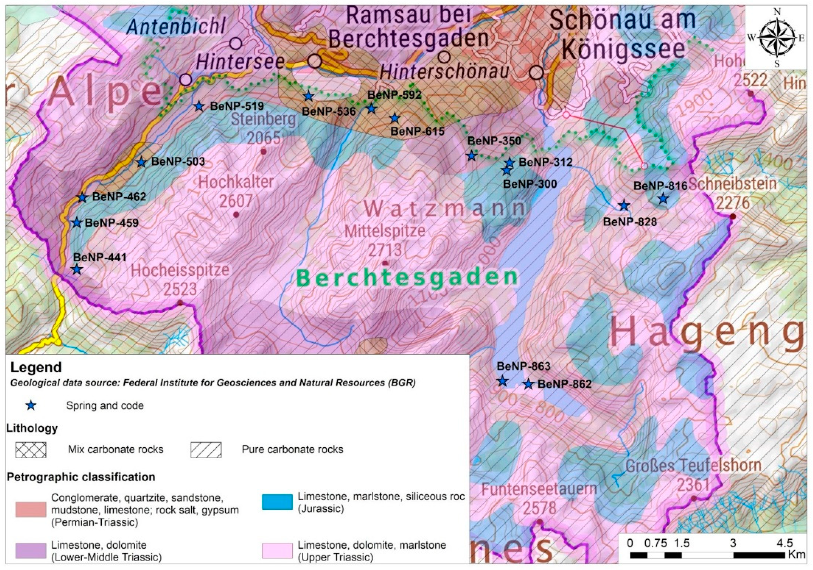
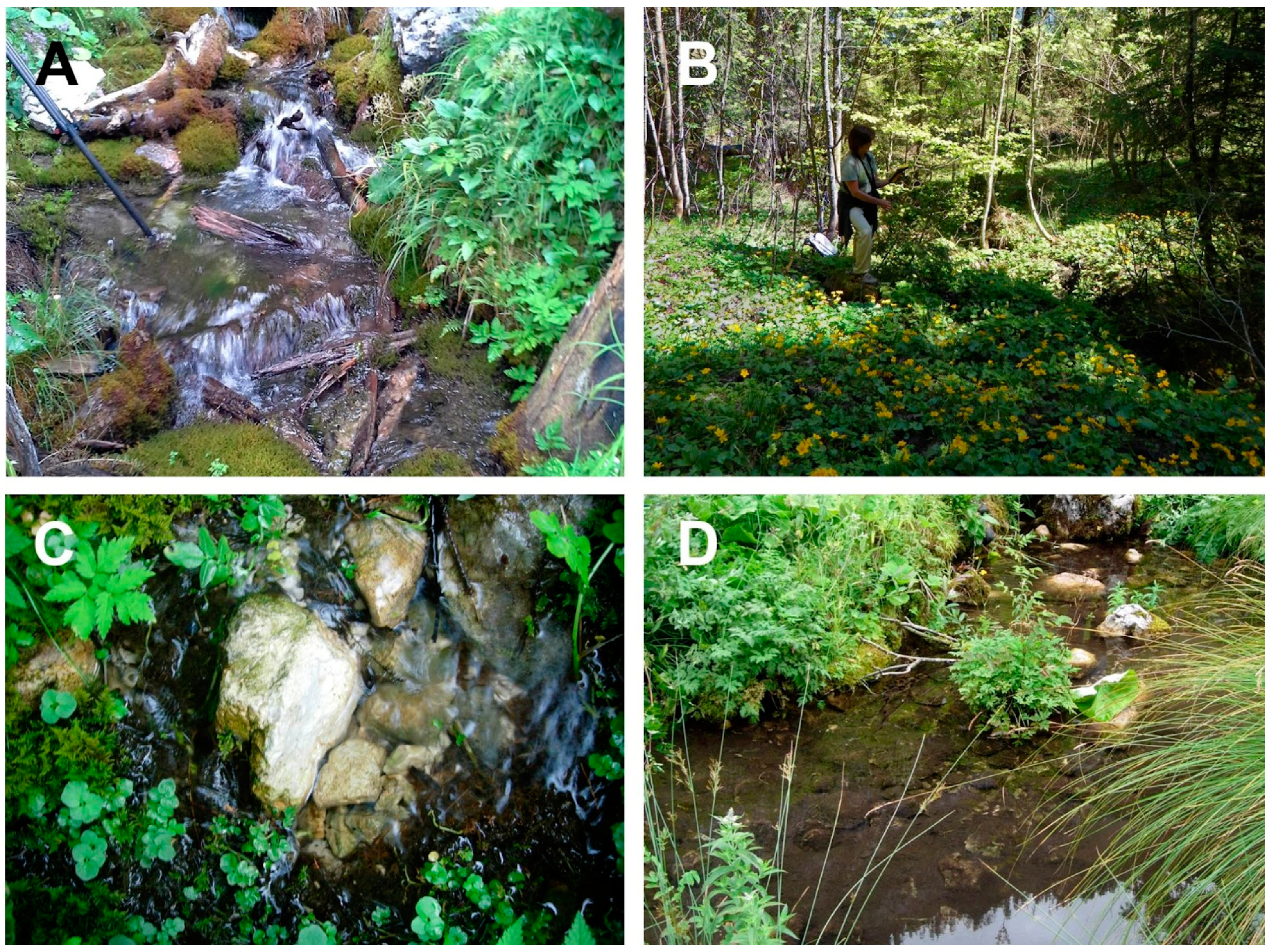
2.1. Study Area

The study area is located in the Berchtesgaden National Park (BeNP), which is the only German National Park in the Alps. Highly productive aquifers are present, characterised by large outcrops of Triassic and Jurassic limestones and dolomites with a thickness of more than 2000 m. The plateaus in the area, which are formed by carbonate rocks, show typical karst phenomena. Permian-Triassic fissured aquifers are also present in the northern part of the Park (Figure 1).

2.2. Field Work & Sampling

The fieldwork/sampling campaign in the BeNP was carried out on 3–7 July 2018. The following parameters were measured: discharge, water temperature, conductivity, pH, dissolved O2, percentage O2, and hydrochemistry (main ions and algal nutrients).
The 33 samples come from different substrata (stones, bryophytes + green filamentous algae, and surface sediment) taken in four kinds of springs. As concerns the rheocrenic type: 2 samples of epiphyton, 3 of epilithon, 3 of epipelon; for the helocrenic type: 1 of epiphyton; with reference to the rheo-limnocrenic type: 2 of epiphyton, 2 of epilithon, 2 of epipelon; finally, for the rheo-helocrenic type: 4 + 1 of epiphyton (4 bryophytes + 1 sample of green filamentous algae), 6 of epilithon, 2 of epipelon.
For three springs (BeNP-312, BeNP-350, BeNP-459), our data could be compared with those based on diatom samples taken on 24–25 June 1997 in the frame of the Spring-Habitat Sampling Workshop (Quellwoche) organised in that year.

2.3. Geology and Hydrogeology

Lithological and geological data used for this work were derived from the Geological Map of Germany 1:1,000,000 and from the 1:5 million International Geological Map of Europe and adjacent areas, developed by the Federal Institute for Geosciences and Natural Resources (BGR) under the umbrella of the Commission of the Geological Map of the World.
A ‘lithology’ variable was defined to express the main composition subdivisions present in the area studied and their influence on the hydrochemistry of the springs studied (details in Table 1).
The springs were classified on the basis of discharge variability using the Meinzer [22] variability index (Rv). This index is a function of the maximum (QM), minimum (Qm), and mean (Qmed) discharge in a hydrological year: Rv = ((QM − Qm)/Qmed)*100). Values of Rv < 25% indicate springs with constant discharge, whereas Rv between 25% and 100% classify a spring as sub-variable. Higher values (Rv > 100%) identify springs with variable discharge. This index was also implemented for temperature and conductivity data.

2.4. Hydrochemistry

Water samples were collected using polyethylene (PE) bottles cleaned with ultra-pure HNO3 (Ultrapure grade, Romil, Cambridge, UK), and rinsed with ultra-pure water (Purelab Ultra Analytic, Elga Lab Water, High Wycombe, UK). Samples for major ions and nutrients were kept chilled (ca. 4 °C) in fridge bags until analysis. Hydrochemical analyses followed standard methodology [23]. Ca2+, Mg2+, Na+, K+, NH4+, Cl, NO3, SO42−, Br, F were analysed by ion chromatography (ICS 1500 Dionex Corp., Sunnyvale, CA, USA), and nutrients (N-NO2, N-NH4+, P-PO43−, TP, TN, Si) by standard absorption spectrometry (details in [10]).

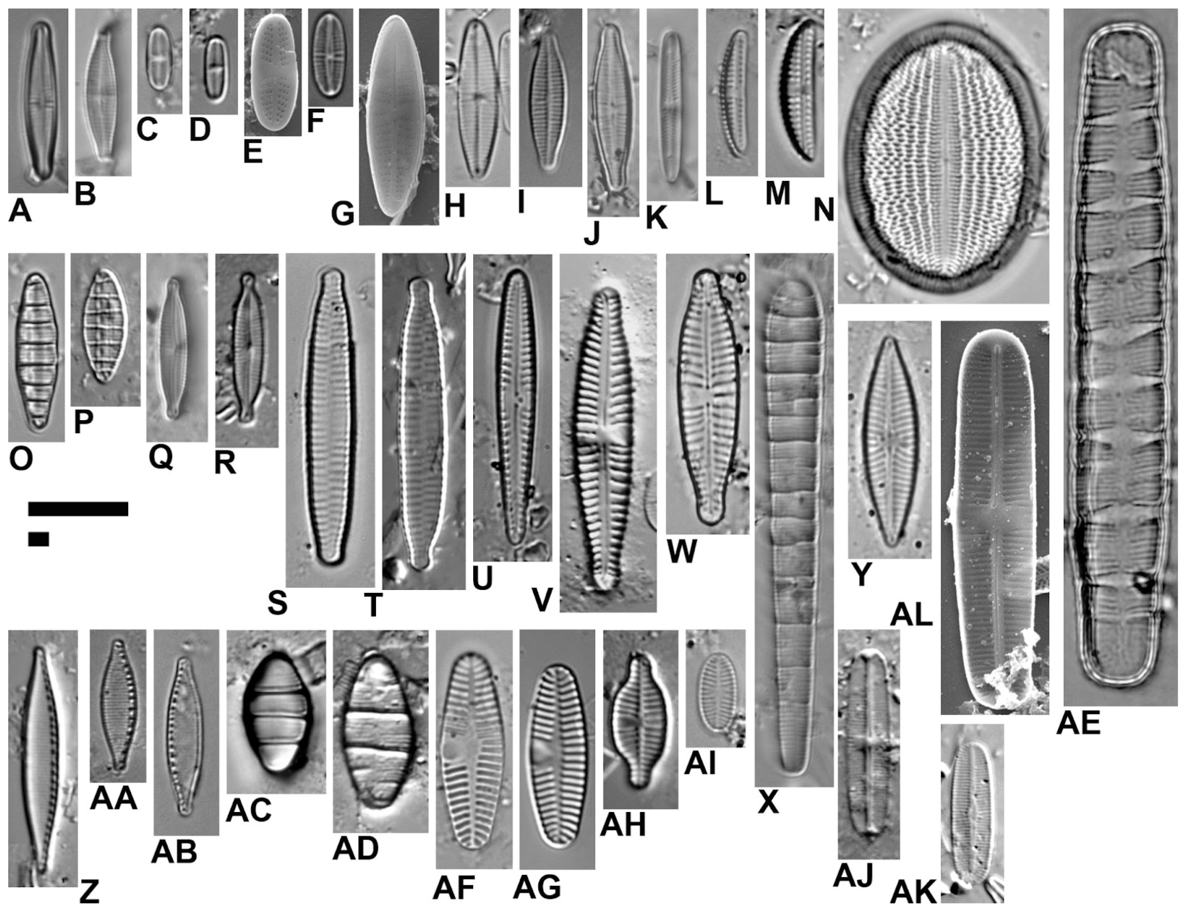
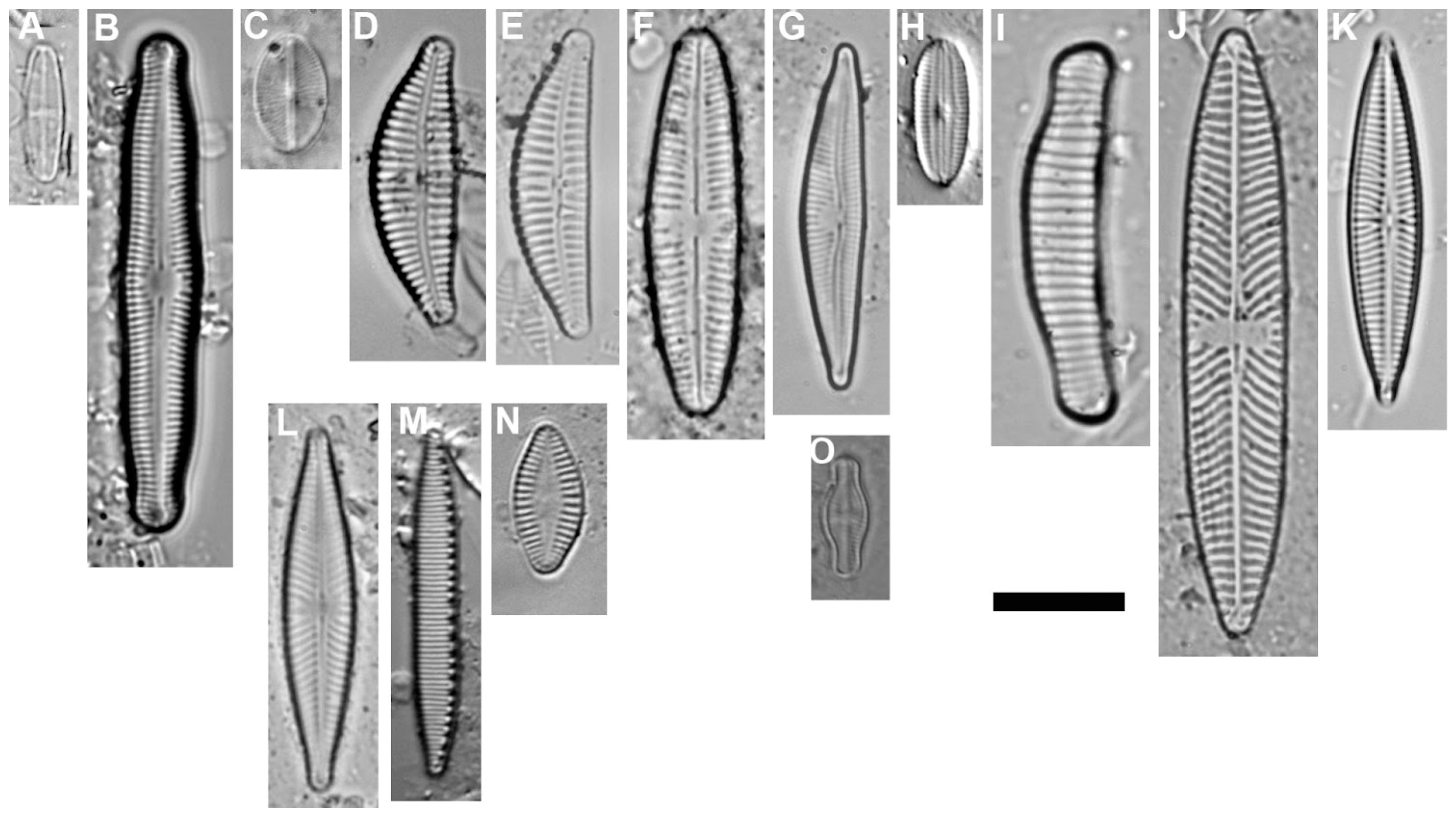
2.5. Diatom Sampling, Identification, and Quantification

Diatom assemblages were sampled and treated following Cantonati et al. [10], with specific designation of the spring-head area (= eucrenal), choice of substrata, and sample preparation. Epilithic diatoms were collected by brushing ten stones. The epibryon (= diatoms living on mosses) was collected from the most frequent and abundant bryophytes in each sample location. Epipelic diatoms (= on surface sediment, upper few mm) were sampled using a large bore syringe. The collected materials, including the bryophytes, were cut into small pieces and were digested using hydrogen peroxide [10]. The cleaned material was mounted in Naphrax (refractive index of 1.74). For each sample, three cover-slips were prepared on one permanent slide, and a pooled total of 400 valves were counted. All slides were then scanned for taxa with low relative abundances for several hours. All samples (original samples, suspensions of digested material, and permanent mounts) have been catalogued and deposited in the collections of the MUSE—Museo delle Scienze (Trento) (access codes: cLIM007 DIAT 3469-3512) along with information about the abundance of the species found and the main environmental variables.
Counting was conducted with a Zeiss Axioskop 2 at ×1000 magnification (Zeiss, Oberkochen, Germany). The most updated taxonomy and nomenclature was applied, and identification reference works were as in Cantonati et al. [10]. Also the following were consulted: Cantonati et al. [24], AlgaeBase [25], DiatomBase [26], Diatoms of North America [27], the Freshwater Diatom Flora of Britain and Ireland [28]. To confirm identifications and document taxa with poorly-observed ultrastructure, several taxa were examined with SEM (Zeiss-EVO40XVP, Carl Zeiss SMT Ltd., Cambridge, UK) at the MUSE—Museo delle Scienze (Trento) at high vacuum on gold-coated stubs.

2.6. Bryophytes

Within the springhead, the bryophyte species submerged or closest to the water were collected from three spots, with the main goal to study the epiphytic diatoms (diatom epibryon). Species nomenclature follows Hodgetts et al. [29]. For all bryophyte species collected in this study, a threat status was assigned according to current [30] and previous Red List data [31]. The habitat preferences of the species were obtained from the dataset BRYOATT [32].

2.7. Data Processing and Statistical Analyses

A threat status (used also as a measure of rarity) was assigned to all diatom species, according to current [6] and previous Red List data [12]. Hofmann et al. [6] provide further ecological attributes (trophic and mineralization preferences, aerial species) used in this study. Preferences of the individual taxa with respect to moisture, trophic state, nitrate content, and pH were obtained from Van Dam et al. [33] and Rott et al. [34].
Shannon-Wiener diversity [35] was calculated using a base-2 logarithm. Canonical Correspondence Analysis (CCA) was carried out with the R [36] package vegan [37]. CCA was selected over other ordination techniques, after evaluation of the length of the gradient. Model selection was performed with the orddistep function of vegan, with an automatic, stepwise model with constrained ordination. The significance of the CCA model was tested with an ANOVA-like permutation test (999 permutations). Ordination of samples was performed using the Nonmetric Multidimensional Scaling (NMDS) and the Bray-Curtis dissimilarity index. The NMDS was performed using all the available diatom samples (1997 and 2018 using all the substrates) in order to inspect if any segregation was present in the community data. In addition, we tested possible differences among factors using a permutational multivariate analysis of variance using distance matrices (a.k.a. Adonis in the vegan package).

3. Results

3.1. Morphological, Physical, and Chemical Characterization of the Springs Studied

The 15 springs considered for this work (Table 1) were: Sommerbichel—source area N Herrenroint, top source (point a) (Watzmann-Nord) (BeNP-300) and headwaters N Herrenroint, lower helocrene (point d) (Watzmann-Nord) (BeNP-312); Schapbach source (Watzmann-North) (BeNP-350); source between Mittereisalm and Hirschbichl (Klaustal-Hintersee) (BeNP-441); Engertalm, rheocrene 1 and Klauswandl (Klaustal-Hintersee) (BeNP-459) and source on the right bank of Klausbach (Klaustal-Hintersee) (BeNP-462); Schwarzbrunnen, western source (Klaustal-Hintersee) (BeNP-503); Klausbach, source flowing from N oh Hintersee (Klaustal-Hintersee) (BeNP-519); Eckau, source in the Eckaugraben (Klaustal-Hintersee) (BeNP-536); rheocrene near Bartler, Wimbachklamm S-exit (Wimbach) (BeNP-592); Koppenwand, source area exposure NW, rheocrene (Wimbach) (BeNP-615); western spring NE Bärenwand (Königssee-Ost) Königsbach-Alm (BeNP-816), source to the left of BGL 826, SO Holzstube (Königssee-Ost) (BeNP-828); Salet-Alm, source between the Obersee and Königssee outflow (Königssee West-Steinernes Meer) (BeNP-862); limnocrene with drain below Sagereckwand (Königssee West-Steinernes Meer) (BeNP-863).
The springs studied are located at medium to low elevations (from c. 600 to c. 1600 m a.s.l.), and were assigned to ecomorphological types as follows: 4 rheocrenes (BeNP-350, BeNP-459, BeNP-503, BeNP-592; Figure 2A); 1 helocrene (BeNP-312; Figure 2B); 8 rheo-helocrenes (BeNP-300, BeNP-441, BeNP-462, BeNP-519, BeNP-536, BeNP-615, BeNP-816, BeNP-828; Figure 2C); 2 rheo-limnocrenes (BeNP-862, BeNP-863; Figure 2D).
Conductivity (average values ranging from 152 to 377 μS cm−1) and pH (average values ranging from 7.65 to 8.39) were consistent with the carbonate substratum. Sulphate values were medium to low (mostly 1–4 mg L−1). Low chloride values suggested an absence of contamination for most of the sites. Nitrates (average values ranging from 1.35 to 7.14 mg L−1) were mostly compatible with an oligotrophic status but still somewhat increased in several sites (Table 1).
Table 2 provides a comparison of the main physical and chemical factors and parameters for the three springs studied in the Berchtesgaden National Park for which also older (1997) diatom data were available. Also, basic key parameters for the tracking of climate change, such as water temperature, discharge, and conductivity show recent (2018) values which are remarkably similar to those measured in 1997.

3.2. Bryophytes (Sampled to Study Epiphytic Diatoms)

The most common moss was Palustriella commutata (Hedw.) Ochyra (Table 3), a eurasiatic species normally found in mineral-rich springs on carbonate substrata, under relatively mild climatic conditions. It is regarded as the only character species of the association Cratoneuretum commutati Aichinger to which most of the springs studied here probably belong. Associated species can be Bryum pseudotriquetrum (Hedw.) G.Gaertn. et al., which was usually found in sunlit habitats as those recorded in BeNP-300 and BeNP-816. Cratoneuron filicinum (Hedw.) Spruce, Palustriella falcata (Brid.) Hedenäs and P. decipiens (De Not.) Ochyra are again species commonly found associated with Palustriella commutata. The phytocoenon of Cratoneuron filicinum (Hedw.) Spruce is a mostly colline crenic vegetation, sometimes occurring at anthropogenically disturbed sites. The dominant moss is relatively common at lower elevations, and it seems to be characteristic of somewhat eutrophic waters. Palustriella falcata, is a circumboreal species that can colonise irrigated calcareous rocks, springs, and fens often at a higher altitude than P. commutata. Rhizomnium punctatum (Hedw.) T.J. Kop. can be common on the mountains of Central Europe, where it colonises montane springs in shaded situations.

3.3. Diatom Species Found in the Different Spring Types and on the Different Substrata

In some samples the diatoms’ amounts were very low, making them incompatible with quantitative or semi-quantitative, and sometimes even with qualitative analysis. During preliminary observations of the permanent mounts, on the sample from Schwarzbrunnen, westliche Quelle (Klaustal-Hintersee) (BGL_503) and Klausbach, source flowing from N upstream Hintersee (Klaustal-Hintersee) (BGL_519), the diatoms were found to be virtually absent. Therefore, these samples could not be considered.
A total of 162 diatom species belonging to 49 genera was found in the three habitat types (epiphytic, epilithic, epipelic) of the Berchtesgaden National Park springs sampled in 2018. The findings on the different substratum types were as follows:—bryophytes: 110 species (39 genera);—stones: 95 species (36 genera);—surface sediment: 90 species (37 genera) (Table 4).
In the following, the most abundant and frequent species (relative abundance 10% and more) are presented for each spring type. The rheocrenic springs were colonised mostly by the following species: Achnanthidium jackii Rabenh., A. minutissimum, A. pfisteri Lange-Bert., A. pyrenaicum (Hust.) Kobayasi, A. rostropyrenaicum Jüttner & Cox, Amphora micra Levkov, Nitzschia fonticola Grunow, Odontidium mesodon (Ehrenb.) Ralfs, Planothidium lanceolatum (Bréb. ex Kütz.) Lange-Bert., P. reichardtii Lange-Bert. et Werum & Lange-Bert. (Figure 3). The most abundant species in helocrenic springs were A. minutissimum and Navicula cryptotenella Lange-Bert. whilst the most abundant species rheo-limnocrenic springs were: A. minutissimum, Denticula tenuis Kütz., and Rossithidium petersenii (Hust.) Round et Bukhtiyarova. The species most abundant in the most common spring type of the present study, i.e., rheohelocrenes, were as follows: Achnanthidium lineare W. Smith, A. minutissimum, A. pfisteri, A. pyrenaicum, A. rostropyrenaicum, A. sublineare Van de Vijver, Jarlman & Ector, Amphora micra, A. pediculus (Kütz.) Grunow, Cocconeis lineata Ehrenb., Denticula tenuis, Encyonopsis krammeri E.Reichardt, Fragilaria vaucheriae (Kütz.) J.B.Petersen, Gomphonema elegantissimum E.Reichardt et Lange-Bert., G. micropus Kütz., Meridion circulare (Gréville) C. Agardh, Nitzschia perminuta (Grunow) H. Perag., Odontidium mesodon, O. neomaximum Jüttner et al., Planothidium lanceolatum, Psammothidium grischunum (Wuthrich) Bukhtiyarova et Round.

3.4. Red-List Species

Red List [6] status was available for 83% (134 out of 162) of the taxa. The distribution of these species in the threat categories was found to be as follows: 7% “2” (=strongly threatened), 9% “3” (=threatened), 14% “G” (=threat of unknown extent), 2% “R” (=extremely rare), 6% “V” (=declining), 12% “D” (=data insufficient), 50% “*” (=not threatened). Several characteristic, rare, and Red-List species are shown in Figure 4.
The nine species classified as “2” were: Achnanthidium dolomiticum, Cymbella affinis Kütz, C. tridentina Lange-Bert., Cantonati et A.Scalfi, Cymbopleura austriaca (Grunow) Krammer, Eunotia arcubus Nörpel et Lange-Bert., Navicula dealpina Lange-Bert., N. wildii Lange-Bert., Sellaphora schadei (Krasske) C.E.Wetzel, Ector, Van de Vijver, Compère et D.G.Mann, S. stroemii (Hust.) D.G.Mann.
The 11 species classified as “3” were: Caloneis tenuis (W.Greg.) Krammer [39], Cavinula jaernefeltii (Hust.) D.G. Mann et Stickle, Cymbella vulgata Krammer [40], Cymbopleura subaequalis (Grunow) Krammer, Delicata delicatula (Kütz.) Krammer, Diploneis petersenii Hust., Navicula subalpina E.Reichardt, Nitzschia alpina Hust., Platessa montana (Krasske) Lange-Bert., Rossithidium petersenii, Stauroforma exiguiformis (Lange-Bert.) Flower, Jones et Round.
Of the 15 species with data insufficient, the following can be classified to be oligotraphentic (and thus sensitive) (“Do”) on the basis of experience and literature: Amphora micra, Cymbopleura korana Krammer, Humidophila paracontenta (Lange-Bert. et Werum) Lowe, Kociolek, Johansen, Van de Vijver, Lange-Bert. et Kopalová. Of the 35 species not present in the current Red List [6], the following can be assigned to threat categories as follows on the basis of experience and literature: Achnanthidium rostropyrenaicum (G), A. sublineare (R), Cymbella diminuta (Grunow) Krammer (3), Encyonopsis fonticola (Hust.) Krammer (3), Geissleria gereckei Cantonati & Lange-Bert. (2) [41], Gomphonema sarcophagus W.Greg (R), Odontidium neomaximum (3), Reimeria capitata (Cleve-Euler) Levkov et Ector (R), R. fontinalis Levkov et Ector (R), R. ovata (Hust.) Levkov et Ector (R), Sellaphora gologonica Lai, Ector et C.E.Wetzel (G) [42], S. labernardierei A.Beauger, C.E.Wetzel et Ector (G). In this way, the cumulative percentage of all species included in a threat category including endangered species (2,3,G,R,V,Do) becomes 43%.

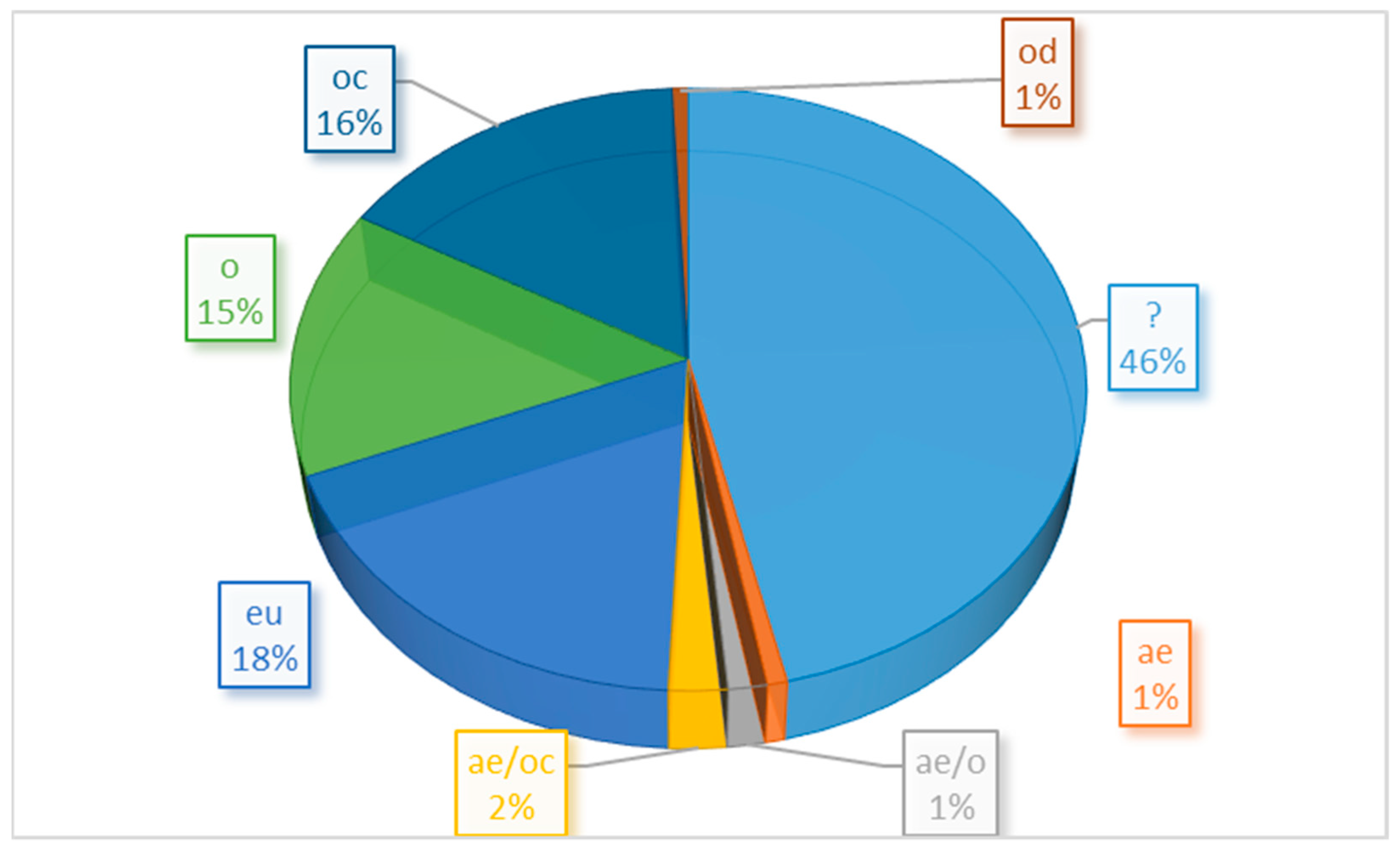
3.5. Ecological Preferences of the Species Found

From the total list of species revealed for fifteen springs of the Berchtesgaden National Park by the sampling campaign in 2018, 138 species (85%) had ecological preferences listed in [6] (Table 3). The indicators distributed among the ecological groups, as shown in Figure 5, included 18% of eutraphentic species and 4% of aerial species.
We also grouped the species list with a focus on moisture preferences (M), as reported in Van Dam et al. [33]. However, these data were available for a limited (about 30%) number of species. Of these, 17% usually can be found on wet and moist or temporarily dry places (group 4), 4% can be observed nearly exclusively outside water bodies (group 5), 46% mainly exist in water bodies, also rather regularly on wet and moist places (group 3), 23% can be observed mainly in water bodies, sometimes on wet places (group 2), and, finally, 10% can be found never, or only very rarely, outside water bodies (group 1) (Figure 6).
Van Dam et al. [33] Trophic state (T) values (not shown) were available for 36% of the diatom species we found. Of these, 26% were eutraphentic, 17% mesotraphentic, 15% oligotraphentic, 14% oligo-mesotraphentic, 14% oligo- to eutraphentic (hypereutraphentic), 12% meso-eutaphentic, and 2% hypereutraphentic. Thus, as can be noted by prevailing indicator taxa of the trophic state, some of the springs studied are obviously affected by some eutrophication impact.

3.6. Relations with Environmental Factors

We could find a statistically significant positive association (r Pearson = 0.733; df = 6, P = 0.038, Figure 7) between the Meinzer variability index for discharge (MVID) and the cumulative relative abundance (sum of percentages) of aerial diatom species (Van Dam et al. [33] moisture categories 4&5 + aerial species “ae” listed in [6]). Even though the relationship was based on a limited number of data, the trend was clear.
The canonical correspondence analysis (CCA) performed between the community data matrix and the environmental factors as constrained variables were not significant, even after deleting the least important variables. The final model, which included water conductivity and magnesium concentration as finally selected variables, was not significant (F = 0.916, P = 0.655).

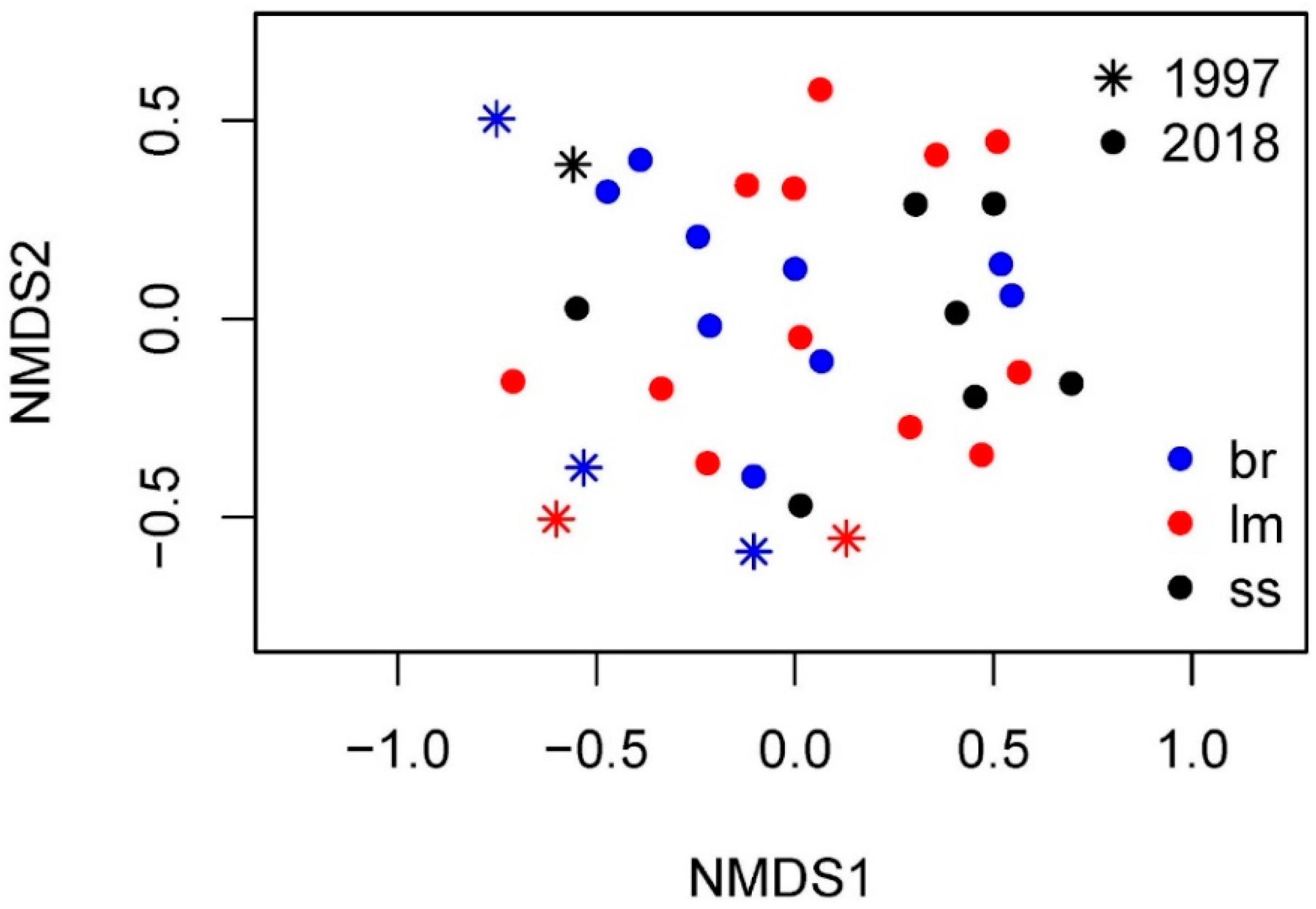
3.7. Comparison with the Data of 1997–1998

Nonmetric Multidimensional Scaling ordination showed that the 1997 samples were partially segregated from those collected in 2018 (asterisks in Figure 8 were all on the left side of the plot). The analysis of variance using Bray Curtis distance matrix and years (1997, 2018), showed that this difference was significant for the factor year (F = 2.109, P = 0.032, Table 4) but not for substrates. This was visually clear also by inspecting the points’ distribution in the NMDS (Figure 8), since bryophyte (br), lithic material (lm), and surface sediment (ss) dots were mixed.
The box and whisker plots in Figure 9, comparing diatom Shannon-Wiener diversity on the three substrata studied, confirm what was seen in the results of the Nonmetric Multidimensional Scaling ordination (Figure 8) and confirmed by the analysis of variance using Bray Curtis distance matrix (Table 5), i.e., that differences were significant for the factor year but not for substrata. In spite of this, the box plots hint at higher diversity in the epibryon diatom assemblages. The higher diversity of the surface sediment could be an artefact: the method that we used indeed does not allow us to distinguish cells living at the time of sampling from dead and empty frustules that typically accumulate in the deposition zones where surface sediment is found (Figure 9).

4. Discussion

This study confirmed the relevance of discharge (and associated water-level) variability as an environmental determinant of diatom assemblages in spring ecosystems. In particular, we could demonstrate a statistically significant relationship (positive association) between discharge variability (Meinzer variability index for discharge) and the cumulative percentage of aerial diatom species. We found 21% of species belonging to categories 4+5 of the Van Dam et al. [33] moisture index, which is in perfect agreement of 20–25% of such species reported for springs of the Alps by Cantonati et al. [10]. Besides well-known aerial species, we found other diatoms typical of freshwater environments with fluctuating discharge and water levels, such as Achnanthidium dolomiticum [10,16], Denticula tenuis [43], Eunotia arcubus [10], Geissleria gereckei [44], Meridion circulare [10], Planothidium frequentissimum (Lange-Bert.) Lange-Bert. [10].
Hydrology, and in particular discharge and its variability, has recently been pointed out as an environmental factor of overwhelming importance in structuring diatom assemblages, e.g., in the Mediterranean [45] and Neotropical [46] streams. Cantonati et al. [11] found higher than expected proportions of diatom species in threat categories of the Red List in the Van Dam et al. [33] moisture categories 4+5, which include most aerial species and attributed this to the fact that diatoms from subaerial habitats (soils, etc.) were less studied and surveyed than those from frankly aquatic environments.
In spring habitats, Taxböck et al. [47] found that discharge was an important variable influencing diatom specie richness along elevational gradients and that higher flow rates tended to lead to higher similarities among diatom communities developing on different substrata (= in different microhabitats within a spring). Cantonati et al. [48] noted that the relevance of discharge variability sometimes tends to be underestimated in spring investigations because permanent, stable springs are often selected for this type of study.
Considering that two of the most important possible effects of climate change are warming and reduction of precipitations, discharge is also a key variable in the few studies using spring ecosystems and their biota as sentinels of environmental change [21]. Though in our study data collected more than twenty years ago were limited to three springs only, our results still show a segregation of the older data in non-parametric diatom-based ordinations, suggesting a strong potential for the use of spring diatoms in studies aiming at tracking the effects of climate and environmental change.
Finally, our study confirmed important, meanwhile well-known features [e.g., 10] of diatom assemblages in Alpine spring ecotones:
-
a relevant occurrence of eutraphentic diatom species and reduction in taxa number and diversity in some springs (compare [20]), resulting from increased nitrate concentrations, likely due to diffuse airborne pollution or local impacts such as forest management, game, and cattle;
-
an important occurrence of species included in threat categories of the diatom Red List ([6,12]) in springs on carbonate substrata (40–50%, [10,11]);
-
a higher species richness on bryophytes (compare [10]), suggesting this substratum to be best suitable for studies focussing on biodiversity inventories (whilst stones should be preferred to investigate relationships between diatom assemblages and hydrochemistry).

Author Contributions

Conceptualization, M.C. and R.G.; Data curation, M.C., O.B., D.S., N.A., S.S., D.B., K.L. and A.A.S.; Formal analysis, D.S.; Funding acquisition, M.C., K.L. and R.G.; Investigation, M.C., R.G. and A.A.S.; Methodology, M.C., D.B., K.L. and R.G.; Project administration, M.C., K.L. and R.G.; Resources, M.C., S.S. and R.G.; Supervision, M.C.; Validation, M.C., N.A., S.S., R.G. and A.A.S.; Visualization, M.C., O.B., D.S., N.A. and D.B.; Writing—original draft, M.C., O.B., S.S. and A.A.S.; Writing—review & editing, M.C., O.B., D.S. and R.G. All authors have read and agreed to the published version of the manuscript.

Funding

This study was carried out in the frame of the Project “Springs in the Bavarian National Parks as indicators of climate change—QuellNPB; TKP01KPB-70869 and TKP01KPB-71382“ financed and supported by the Bavarian State Ministry for the Environment and Consumer Protection.

Data Availability Statement

Data are available upon request from the Authors and from the Berchtesgaden National Park Administration.

Acknowledgments

We are grateful to the Bavarian State Ministry for the Environment and Consumer Protection and the Nationalpark Berchtesgaden for support, to Gabriele Leonhardt for indispensable assistance during field work, and to Claire Pfalzner-Gibbon (Berchtesgaden National Park), and Elmar Pröll (Kalkalpen National Park, Austria) for making available the results of comprehensive hydrochemical analysis.

Conflicts of Interest

The authors declare no conflict of interest.

References

  1. Mann, D.G.; Vanormelingen, P. An Inordinate Fondness? The Number, Distributions, and Origins of Diatom Species. J. Eukaryot. Microbiol. 2013, 60, 414–420. [Google Scholar] [CrossRef] [PubMed] [Green Version]
  2. Mann, D.G. The species concept in diatoms. Phycological. Reviews 18. Phycologia 1999, 38, 437–495. [Google Scholar] [CrossRef] [Green Version]
  3. Smol, J.P.; Stoermer, E.F. The Diatoms: Applications for the Environmental and Earth Sciences, 2nd ed.; Cambridge University Press: Cambridge, UK, 2010; pp. 1–667. [Google Scholar]
  4. Lange-Bertalot, H.; Metzeltin, D. Indicators of Oligotrophy. 2. In Iconogr. Diatomol; Lange-Bertalot, H., Ed.; Koeltz Scientific Books: Königstein, Germany, 1996; pp. 1–390. [Google Scholar]
  5. Cantonati, M.; Füreder, L.; Gerecke, R.; Jüttner, I.; Cox, E.J. Crenic habitats, hotspots for freshwater biodiversity conservation: Toward an understanding of their ecology. Freshw. Sci. 2012, 31, 463–480. [Google Scholar] [CrossRef]
  6. Hofmann, G.; Lange-Bertalot, H.; Werum, M.; Klee, R.; unter Mitarbeit von König, C.; Kusber, W.-H.; Metzeltin, D.; Reichardt, E. Rote Liste und Gesamtartenliste der limnischen Kieselalgen (Bacillariophyta) Deutschlands. In Rote Liste Gefährdeter Tiere, Pflanzen und Pilze Deutschlands; Metzing, D., Hofbauer, N., Ludwig, G., Matzke Hajek, G., Eds.; Band 7; Naturschutz und Biologische Vielfalt 70; Landwirtschaftsverlag: Münster, Germany, 2018; pp. 601–708. [Google Scholar]
  7. Moser, G.; Lange-Bertalot, H.; Metzeltin, D. Insel der Endemiten Geobotanisches Phänomen Neukaledonien (Island of endemics New Caledonia—A geobotanical phenomenon); Bibliotheca Diatomologica 38; J. Cramer: Berlin/Stuttgart, Germany, 1998; pp. 1–464. [Google Scholar]
  8. Kociolek, J.P.; Stoermer, E.F. Oligotrophy: The forgotten end of an ecological spectrum. Proceedings of the 20th International Diatom Symposium (Dubrovnik, Croatia). Acta Bot. Croat. 2009, 68, 465–472. [Google Scholar]
  9. Lowe, W.H.; Likens, G.E. Moving headwater streams to the head of the class. BioScience 2005, 55, 196–197. [Google Scholar] [CrossRef] [Green Version]
  10. Cantonati, M.; Angeli, N.; Bertuzzi, E.; Spitale, D.; Lange-Bertalot, H. Diatoms in springs of the Alps: Spring types, environmental determinants, and substratum. Freshw. Sci. 2012, 31, 499–524. [Google Scholar] [CrossRef]
  11. Cantonati, M.; Hofmann, G.; Spitale, D.; Werum, M.; Lange-Bertalot, H. Diatom Red Lists: Important tools to assess and preserve biodiversity and habitats in the face of direct impacts and environmental change. Biodivers. Conserv. 2021, in press. [Google Scholar] [CrossRef]
  12. Lange-Bertalot, H. Rote Liste der Limnischen Kieselalgen (Bacillariophyceae) Deutschlands; 28. Schriftenreihe für Vegetationskunde; Bundesamt fuür Naturschutz: Bonn, Germany, 1996; pp. 633–677.
  13. Taxböck, L.; Linder, H.P.; Cantonati, M. To what extent are Swiss springs refugial habitats for sensitive and endangered diatom taxa? Water 2017, 9, 967. [Google Scholar] [CrossRef] [Green Version]
  14. Cantonati, M.; Virtanen, L.; Angeli, N.; Wojtal, A.; Gabrieli, J.; Falasco, E.; Lavoie, I.; Morin, S.; Marchetto, A.; Fortin, C.; et al. Achnanthidium minutissimum (Bacillariophyta) valve deformities as indicators of metal enrichment in diverse widely-distributed freshwater habitats. Sci. Total Environ. 2014, 475, 201–215. [Google Scholar] [CrossRef]
  15. Cantonati, M.; Lange-Bertalot, H.; Scalfi, A.; Angeli, N. Cymbella tridentina sp. nov. (Bacillariophyta), a crenophilous diatom from carbonate springs of the Alps. J. N. Am. Benthol. Soc. 2010, 29, 775–788. [Google Scholar] [CrossRef]
  16. Cantonati, M.; Lange-Bertalot, H. Achnanthidium dolomiticum sp. nov. (Bacillariophyta) from oligotrophic mountain springs and lakes fed by dolomite aquifers. J. Phycol. 2006, 42, 1184–1188. [Google Scholar] [CrossRef]
  17. Lichtenwöhrer, K.; Leonhardt, G.; Seifert, L.; Hotzy, R.; Schubert, E.; Gerecke, R.; Cantonati, M.; Lotz, A. Erfassung von Klimawandelfolgen an Quellen in Bayern. Leitfaden für eine langfristige Beobachtung von Quellen zur Erfassung von Klimawandelfolgen in Bayern. Nationalpark Berchtesgaden und Nationalpark Bayerischer Wald. Auf Vorgabe des Bayerischen Umweltministeriums. Entwurf zur praktischen Evaluierung und wissenschaftlichen Kommentierung. Bayern, Germany. 2020, pp. 1–71. Available online: https://www.nationalpark-bayerischer-wald.bayern.de/forschung/projekte/doc/leitfaden_quellbeobachtung.pdf (accessed on 7 November 2021).
  18. Lotter, A.F.; Pienitz, R.; Schmidt, R. Diatoms as indicators of environmental change in subarctic and alpine regions. In The Diatoms: Applications for the Environmental and Earth Sciences, 2nd ed.; Smol, J.P., Stoermer, E.F., Eds.; Cambridge University Press: Cambridge, UK, 2010; pp. 231–248. [Google Scholar] [CrossRef]
  19. Bahls, L.; Pierce, J.; Apfelbeck, R.; Olsen, L. Encyonema droseraphilum sp. nov. (Bacillariophyta) and other rare diatoms from undisturbed floating-mat fens in the northern Rocky Mountains, USA. Phytotaxa 2013, 127, 32–48. [Google Scholar] [CrossRef] [Green Version]
  20. Cantonati, M.; Lange-Bertalot, H. Diatom biodiversity of springs in the Berchtesgaden National Park (North-Eastern Alps, Germany), with the ecological and morphological characterization of two species new to science. Diatom Res. 2010, 25, 251–280. [Google Scholar] [CrossRef]
  21. Gerecke, R.; Cantonati, M.; Spitale, D.; Stur, E.; Wiedenbrug, S. The challenges of long-term ecological research in springs in the northern and southern Alps: Indicator groups, habitat diversity, and medium term change. J. Limnol. 2011, 70 (Suppl. 1), 168–187. [Google Scholar] [CrossRef]
  22. Meinzer, O.E. Outline of Ground-Water Hydrology; Water Supply Paper; Department of the Interior, U.S. Geological Survey. Washington Government Printing Office: Washington, DC, USA, 1923; p. 494.
  23. Standard Methods for the Examination of Water and Wastewater, 20th ed.; APHA, AWWA & WEF, American Public Health Association: Washington, DC, USA, 2000; pp. 1–541.
  24. Cantonati, M.; Kelly, M.G.; Lange-Bertalot, H. (Eds.) Freshwater Benthic Diatoms of Central Europe: Over 800 Common Species Used in Ecological Assessment; Koeltz Botanical Books: Schmitten-Oberreifenberg, Germany, 2017; pp. 1–942. [Google Scholar]
  25. Guiry, M.D.; Guiry, G.M. AlgaeBase. World-Wide Electronic Publication, National University of Ireland, Galway. Available online: https://www.algaebase.org (accessed on 29 December 2021).
  26. Kociolek, J.P.; Balasubramanian, K.; Blanco, S.; Coste, M.; Ector, L.; Liu, Y.; Kulikovskiy, M.; Lundholm, N.; Ludwig, T.; Potapova, M.; et al. DiatomBase. 2021. Available online: http://www.diatombase.org (accessed on 29 December 2021).
  27. Spaulding, S.A.; Bishop, I.W.; Edlund, M.B.; Lee, S.; Furey, P.; Jovanovska, E.; Potapova, M. Diatoms of North America. 2020. Available online: https://diatoms.org (accessed on 30 December 2021).
  28. Jüttner, I.; Carter, C.; Chudaev, D.; Cox, E.J.; Ector, L.; Jones, V.; Kelly, M.G.; Kennedy, B.; Mann, D.G.; Turner, J.A.; et al. Freshwater Diatom Flora of Britain and Ireland. Amgueddfa Cymru–National Museum Wales. 2021. Available online: https://naturalhistory.museumwales.ac.uk/diatoms (accessed on 30 December 2021).
  29. Hodgetts, N.G.; Hodgetts, N.G.; Soderstrom, L.; Blockeel, T.L.; Caspari, S.; Ignatov, M.S.; Konstantinova, N.A.; Lockhart, N.; Papp, B.; Schrock, C.; et al. An annotated checklist of bryophytes of Europe, Macaronesia and Cyprus. J. Bryol. 2020, 42, 1–116. [Google Scholar] [CrossRef]
  30. Caspari, S.; Dürhammer, O.; Sauer, M.; Schmidt, C. Rote Liste und Gesamtartenliste der Moose (Anthocerotophyta, Marchantiophyta und Bryophyta) Deutschlands. In Rote Liste gefährdeter Tiere, Pflanzen und Pilze Deutschlands; Band 7: Pflanzen; Metzing, D., Hofbauer, N., Ludwig, G., Matzke-Hajek, G., Eds.; Münster (Landwirtschaftsverlag): Münster, Germany, 2018; Volume 70, pp. 361–489. [Google Scholar]
  31. Ludwig, G.; Düll, R.; Philippi, G.; Ahrens, M.; Caspari, S.; Koperski, M.; Lütt, S.; Schulz, F.; Schwab, G. Rote Liste der Moose (Anthocerophyta et Bryophyta) Deutschlands. In Rote Listen gefährdeter Pflanzen Deutschlands; Ludwig, G., Schnittler, M., Eds.; 28. Schriftenreihe für Vegetationskunde; Bundesamt fuür Naturschutz: Bonn, Germany, 1996; pp. 189–306. [Google Scholar]
  32. Hill, M.O.; Preston, C.D.; Bosanquet, S.D.S.; Roy, D.B. BRYOATT: Attributes of British and Irish Mosses, Liverworts and Hornworts; Software (updated 2017); Centre for Ecology and Hydrology: Lancaster, UK, 2007. [Google Scholar]
  33. Van Dam, H.; Mertens, A.; Sinkeldam, J. A coded checklist and ecological indicator values of freshwater diatoms from the Netherlands. Neth. J. Aquat. Ecol. 1994, 28, 117–133. [Google Scholar]
  34. Rott, E.; Pipp, E.; Pfister, P.; Van Dam, H.; Ortler, K.; Binder, N.; Pall, K. Indikationslisten für Aufwuchsalgen in österreichischen Fliessgewässern. Teil 2: Trophieindikation (Sowie Geochemische Präferenzen, Taxonomische und Toxikologische Anmerkungen). Wasserwirtschaftskataster, Bundesministerium f. Land-u; Forstwirtschaft: Vienna, Austria, 1999; pp. 1–248. [Google Scholar]
  35. Shannon, C.E. A mathematical theory of communication. Bell Syst. Tech. J. 1948, 27, 37–42. [Google Scholar] [CrossRef] [Green Version]
  36. R Core Team. R: A Language and Environment for Statistical Computing; R Foundation for Statistical Computing: Vienna, Austria, 2018; Available online: https://www.R-project.org (accessed on 7 March 2003).
  37. Oksanen, J.; Guillaume Blanchet, F.; Friendly, M.; Kindt, R.; Legendre, P.; McGlinn, D.; Minchin, P.R.; O’Hara, R.B.; Simpson, G.L.; Solymos, P.; et al. Vegan, R Package Version 2.5–6; Community Ecology Package; R Foundation for Statistical Computing: Vienna, Austria, 2019. [Google Scholar]
  38. Ellenberg, H.; Weber, H.E.; Düll, R.; Wirth, V.; Werner, W.; Paulißen, D. Zeigerwerte von Pflanzen in Mitteleuropa. Scr. Geobot. 1991, 18, 1–248. [Google Scholar]
  39. Krammer, K.; Lange-Bertalot, H. Bacillariophyceae. 1. Teil: Naviculaceae. In Süsswasserflora von Mitteleuropa, Band 2/1; Ettl, H., Gerloff, J., Heynig, H., Mollenhauer, D., Eds.; Gustav Fisher Verlag: Jena, Germany, 1986; pp. 1–876. [Google Scholar]
  40. Krammer, K. Cymbella. In Diatoms of Europe; Lange-Bertalot, H., Ed.; J. Cramer: Berlin/Stuttgart, Germany, 2002; Volume 3, pp. 1–584. [Google Scholar]
  41. Cantonati, M.; Spitale, D. The role of environmental variables in structuring epiphytic and epilithic diatom assemblages in springs and streams of the Dolomiti Bellunesi National Park (south-eastern Alps). Fundam. Appl. Limnol. Arch. Hydrobiol. 2009, 1742, 117–133. [Google Scholar] [CrossRef]
  42. Lai, G.G.; Ector, L.; Lugliè, A.; Sechi, N.; Wetzel, C.E. Sellaphora gologonica sp. nov. (Bacillariophyta, Sellaphoraceae), a new diatom species from a Mediterranean karst spring (Sardinia, Italy). Phytotaxa 2018, 356, 145–157. [Google Scholar] [CrossRef]
  43. Cantonati, M.; Scola, S.; Angeli, N.; Guella, G.; Frassanito, R. Environmental controls of epilithic diatom depth-distribution in an oligotrophic lake characterised by marked water-level fluctuations. Eur. J. Phycol. 2009, 44, 15–29. [Google Scholar] [CrossRef]
  44. Vidaković, D.; Cantonati, M.; Mogna, M.; Jakovljević, O.; Šovran, S.; Lazović, V.; Stojanović, K.; Đorđević, J.; Krizmanić, J. Additional information on the distribution and ecology of the recently described diatom species Geissleria gereckei. Oceanol. Hydrobiol. Stud. 2017, 46, 18–23. [Google Scholar] [CrossRef]
  45. Cantonati, M.; Kelly, M.G.; Demartini, D.; Angeli, N.; Dörflinger, G.; Papatheodoulou, A.; Armanini, D. Overwhelming role of hydrology-related variables and river types in driving diatom species distribution and community assemblage in streams in Cyprus. Ecol. Indic. 2020, 117, 106690. [Google Scholar] [CrossRef]
  46. Rondón, J.C.D.; Aragón, Y.A.A. Factors driving diversity and succession of diatom assemblages in a Neotropical rainforest stream. Ann. Limnol. Int. J. Lim. 2018, 54, 30. [Google Scholar] [CrossRef]
  47. Taxböck, L.; Karger, D.N.; Kessler, M.; Spitale, D.; Cantonati, M. Diatom species richness in Swiss Springs Increases with Habitat Complexity and Elevation. Water 2020, 12, 449. [Google Scholar] [CrossRef] [Green Version]
  48. Cantonati, M.; Segadelli, S.; Spitale, S.; Gabrieli, J.; Gerecke, R.; Angeli, N.; De Nardo, M.T.; Ogata, K.; Wehr, J.D. Geological and hydrochemical prerequisites of unexpectedly high biodiversity in spring ecosystems at the landscape level. Sci. Total Environ. 2020, 740, 140157. [Google Scholar] [CrossRef]
Figure 1. Geological map showing the Berchtesgaden National Park with the location of the springs studied.
Water 14 00381 g001
Figure 2. Examples of springs belonging to the four typologies identified: (A) Rheocrenic spring (BeNP-459), (B) Helocrenic spring (BeNP-312), (C) Rheo-helocrenic spring (BeNP-615), (D) Rheo-limnocrenic spring (BeNP-862).
Water 14 00381 g002
Figure 3. Micrographs of the most frequent and abundant species. (A) Achnanthidium minutissimum, (B) Achnanthidium jackii, (CE) Achnanthidium lineare, (F) Achnanthidium pfisteri, (G,H) Achnanthidium pyrenaicum, (I,J) Achnanthidium rostropyrenaicum, (K) Achnanthidium sublineare, (L) Amphora micra, (M) Amphora pediculus, (N) Cocconeis lineata, (O,P) Denticula tenuis, (Q,R) Encyonopsis krammeri, (S,T) Fragilaria pectinalis, (U) Gomphonema elegantissimum, (V,W) Gomphonema micropus, (X) Meridion circulare, (Y) Navicula cryptotenella, (Z)—(AA) Nitzschia fonticola, (AB) Nitzschia perminuta, (AC,AD) Odontidium mesodon, (AE) Odontidium neomaximum, (AF,AG) Planothidium lanceolatum, (AH) Planothidium reichardtii, (AI) Psammothidium grischunum, (AJ,AL) Rossithidium petersenii. (E,G,AL) = SEM; (D,I,P,R,T,V,Z,AD,AG,AH,AJ,AK) = Nomarski (DIC); all the other bright fields. Scale bars: long (LM) 10 µm; short (SEM) 1 µm.
Water 14 00381 g003
Figure 4. Micrographs of characteristic, rare, and Red-List species. (A) Achnanthidium dolomiticum, (B) Caloneis tenuis, (C) Cavinula jaernefeltii, (D) Cymbella affinis, (E) Cymbella tridentina, (F) Cymbopleura subaequalis, (G) Delicata delicatula, (H) Diploneis petersenii, (I) Eunotia arcubus, (J) Navicula dealpina, (K) Navicula subalpina, (L) Navicula wildii, (M) Nitzschia alpina, (N) Platessa montana, (O) Sellaphora sp. aff. schadei. (B,H,M) = Nomarski (DIC); all the other bright field. Scale bar 10 µm.
Water 14 00381 g004
Figure 5. Diatoms of 15 spring habitats in the Berchtesgaden National Park, ecology according to Hofmann et al. [6]: ae—aerial, o—oligotraphentic, oc—oligotraphentic carbonate, od—oligotraphentic distrophic, eu—eutraphentic to tolerant, hal—halophilic, ?—unknown.
Water 14 00381 g005
Figure 6. Moisture (M) groups of diatoms (according to [33]) from spring ecosystems in the Berchtesgaden National Park (Moisture preferences: 1—almost never occurring outside water bodies, 2—mainly occurring in water bodies, sometimes on wet places, 3—mainly occurring in water bodies, also rather regularly on wet and moist places, 4—mainly occurring on wet and moist or temporarily dry places, 5—nearly exclusively occurring outside water bodies).
Water 14 00381 g006
Figure 7. Scatterplot diagram of the positive association between the Meinzer variability index for discharge (MVID) and the cumulative relative abundance (sum of percentages) of aerial diatom species (Van Dam et al. [33] moisture categories 4&5 + aerial species “ae” listed in [6]).
Water 14 00381 g007
Figure 8. Ordination of samples using Nonmetric Multidimensional Scaling of all the samples. br = bryophytes (epiphytic), lm = lithic material (epilithic), ss = surface sediments (epipelic).
Water 14 00381 g008
Figure 9. Boxplot of the Shannon-Wiener diversity of diatoms using as groups the substrates (br = bryophytes, lm = lithic material, ss = surface sediments).
Water 14 00381 g009
Table 1. Morphological, physical, and chemical characteristics of the 15 springs studied in the Berchtesgaden National Park. When several data were available, mean (in bold) and minimum/maximum value are provided. Shading: 1: Springs exposed to full light, but with the presence of tall grass, exposition S, SW or W. 2: Tree-canopy cover, shrubs, rock walls, or other objects, max 25%. 3: Cover from trees, shrubs, rock walls or other objects, max 50%. 4: Shaded by trees and shrubs, max 75%, but SE, S, SW, or W exposition. 5: Heavily shaded by trees and shrubs, > 75%. Pure carbonate rocks (PCR): (L)—Limestone, (M)—marlstone, (D)—dolostone, Mix carbonate rocks (MCR): (CC)—clastic conglomerate, (Q)—quartzite, (CM)—clastic mudstone. Disch. = Discharge. MVID = Meinzer Variability Index for Discharge. MVIT = Meinzer Variability Index for Temperature. MVIC = Meinzer Variability Index for Conductivity.
SPRING CODEBeNP-300BeNP-312BeNP-350BeNP-441BeNP-459BeNP-462BeNP-503BeNP-519BeNP-536BeNP-592BeNP-615BeNP-816BeNP-828BeNP-862BeNP-863
Coordinates47°57′73.92″ N47°57′93.04″ N47°58′16.47″ N47°55′71.19″ N47°56′93.39″ N47°57′58.25″ N47°58′42.57″ N47°59′81.83″ N47°59′93.69″ N47°59′52.7″ N47°59′24.89″ N47°56′78.85″ N47°56′66.04″ N47°52′11.97″ N47°52′23.71″ N
12°97′10.68″ E12°97′23.28″ E12°95′78.32″ E12°80′34.1″ E12°80′42.86″ E12°80′68.39″ E12°83′02.67″ E12°85′36.37″ E12°89′60.88″ E12°92′00.8″ E12°92′88.67″ E13°03′07.77″ E13°01′55.53″ E12°97′51.52″ E12°96′52.67″ E
Altitude, m.a.s.l.1250115011701270110096086080090573088015751200604604
Shading, sc. 1–521–23–43–4244–5354–54–513–421
Spring typeRheo-heloHeloRheoRheo-heloRheoRheo-heloRheoRheo-heloRheo-heloRheoRheo-heloRheo-heloRheo-heloRheo-limnoRheo-limno
LithologyPCR (L, M)PCR (L, M)PCR (L, D)PCR (L, D)PCR (L, M)PCR (L, D)MCR (CC, Q, CM)PCR (L, D)MCR (CC, Q, CM)MCR (CC, Q, CM)MCR (CC, Q, CM)PCR(L, M)PCR (L, D)PCR (L, D)PCR (L, D)
Disch., L s−10.13 (0.01/0.70)0.03 (0.00/0.25)12.89 (2.00/25.0)-23.75 (10.00/50.00)-200 (70.00/500.00)0.19 (0.00/0.75)0.32 (0.01/0.75)3.29 (7.50/70.00)1.83 (0.10/5.00)0.38 (0.05/2.00)--3.92 (1.00/10.00)
MVID531833178-168-2153952311900268513--229
Water T, °C6.85 (5.30/9.40)8.02 (5.70/10.30)5.02 (4.80/5.20)-4.23 (4.00/4.50)-4.68 (4.50/4.90)9.4 (6.70/12.70)8.24 (6.90/9.77)5.41 (5.11/5.92)6.98 (6.01/7.72)6.21 (5.50/6.80)--6.47 (5.88/7.86)
MVIT60.0057.008.00-12.00-8.5064.0035.0015.0024.5021.00--31.00
Cond., µS cm−1341 (295/382)333 (324/346)273 (271/276)347164 (143/183)-155 (129/177)309 (276/331)307 (285/326)192 (168/217)336 (320/351)377 (357/404)283260152 (119/168)
MVIC2672-24-31181326913--32
pH7.72 (7.37/8.14)7.91 (7.74/8.31)7.85 (7.74/8.02)7.698.14 (7.97/8.35)-8.19 (8.02/8.37)8.18 (7.82/8.35)7.81 (7.56/8.07)8.2 (7.95/8.54)7.92 (7.71/8.03)7.65 (7.39/7.89)7.667.738.39 (8.07/8.94)
% O2 sat.87.18 (76.90/94.90)85.54 (73.30/96.80)98.52 (93.00/101.90)92100.13 (96.80/104.90)-100.48 (97.00/103.20)97.01 (92.10/101.00)96.95 (92.80/99.50)98.33 (93.20/103.60)98.2 (93.70/101.40)95.14 (92.80/101.30)9363106.72 (99.70/121.00)
Mg2+, mg L−12.46 (1.98/2.89)1.93 (1.62/2.25)4.34 (3.76/5.03)8.134.96 (3.53/7.68)-487 (3.86/6.15)3.53 (2.43/5.06)6.28 (4.98/7.58)3.92 (2.13/6.28)18.37 (15.57/21.35)8.7 (7.87/9.30)3.183.141.15 (0.55/1.66)
Ca2+, mg L−172.15 (60.01/83.49)69.1 (67.34/71.35)53.23 (50.84/55.08)61.5728.46 (22.94/34.03)-26.94 (21.60/32.28)62.18 (55.23/70.31)57.23 (51.41/61.09)35.62 (29.95/47.02)47.1 (43.54/54.10)73.3 (64.11/88.29)63.4756.8730.51 (24.47/34.69)
Na+, mg L−10.39 (0.14/0.63)0.66 (0.22/1.19)0.51 (0.45/0.54)0.2310.1 (0.04/0.14)-0.09 (0.08/0.12)0.65 (0.44/1.06)0.24 (0.17/0.31)0.14 (0.06/0.31)0.23 (0.10/0.32)0.43 (0.19/0.52)0.530.590.11 (0.04/0.20)
K+, mg L−10.15 (0.05/0.34)0.19 (0.00/0.52)0.19 (0.16/0.23)0.080.06 (0.00/0.11)-0.07 (0.00/0.15)0.4 (0.22/0.66)0.16 (0.09/0.29)0.11 (0.04/0.29)0.17 (0.08/0.26)0.38 (0.20/0.48)0.460.120.06 (0.00/0.13)
Cl, mg L−10.33 (0.15/0.58)0.42 (0.35/0.57)0.42 (0.23/0.71)0.330.2 (0.09/0.42)-0.19 (0.07/0.39)0.39 (0.22/0.65)0.4 (0.19/0.90)0.25 (0.09/0.85)0.42 (0.33/0.78)0.24 (0.08/0.39)0.260.261.13 (0.10/0.18)
NO3, mg L−13.65 (1.33/10.14)1.35 (0.68/2.49)3.52 (2.59/6.38)2.292.22 (1.42/4.68)-2.1 (1.60/3.84)7.14 (4.70/10.89)5.38 (3.49/9.38)3.37 (1.43/9.18)5.13 (3.89/11.32)1.29 (0.02/2.49)3.12.601.6 (0.67/3.34)
SO42−, mg L−13.79 (2.56/7.16)3.96 (3.04/6.08)5.14 (3.78/9.09)0.911.24 (0.67/2.62)-1.3 (0.89/2.42)3.87 (2.67/7.59)2.66 (1.31/5.86)1.53 (0.61/3.29)3.11 (2.29/4.36)1.05 (0.01/1.73)2.191.260.71 (0.34/1.11)
Table 2. Comparison of the main physical, and chemical characteristics of the 3 springs studied in the Berchtesgaden National Park for which also older (1997) diatom data were available. Mean (in bold) and minimum/maximum value.
CODEBeNP-312BeNP-350BeNP-459
Year201819972018199720181997
Disch., L s−10.03 (0.00/0.25)0.0113 (2/25)10 (2/20)24 (10/50)25 (10/40)
Water T, °C8.0 (5.7/10.3)7.7 (5.7/10.3)5.0 (4.8/5.2)5 (4.8/5.1)4.2 (4.0/4.5)4.2 (4.1/4.5)
Cond., µS cm−1333 (324/346)332 (324–346)273 (271/276)273 (271–276)164 (143/183)170 (149–183)
pH7.91 (7.74/8.31)7.8 (7.7–7.9)7.85 (7.74/8.02)7.8 (7.7–7.9)8.14 (7.97/8.35)8.14 (7.97–8.35)
Mg2+, mg L−11.9 (1.6/2.2)1.9 (1.6–2.1)4.3 (3.8/5.03)4.4 (3.8–5.0)5.0 (3.53/7.68)4.9 (4.6–5.9)
Ca2+, mg L−169.1 (67.3/71.3)69.0 (67.3–71.4)53.2 (50.8/55.1)53.7 (52.8–55.1)28.5 (22.9/34.0)29 (25.5–34)
Na+, mg L−10.7 (0.2/1.2)0.6 (0.6–0.7)0.5 (0.4/0.5)0.50.1 (0.04/0.14)0.1
K+, mg L−10.19 (0.00/0.52)0.3 (0.1–0.5)0.19 (0.16/0.23)0.20.06 (0.00/0.11)0.1
Cl, mg L−10.4 (0.3/0.6)0.4 (0.4–0.6)0.4 (0.2/0.7)0.4 (0.2–0.7)0.2 (0.1/0.4)0.2 (0.1–0.4)
NO3, mg L−11.35 (0.68/2.49)1.0 (0.8–1.9)3.52 (2.59/6.38)2.8 (2.7–6.4)2.22 (1.42/4.68)2.0 (1.4–4.7)
SO42−, mg L−14.0 (3.0/6.1)3.7 (3.6–4.0)5.1 (3.8/9.1)4.3 (3.9–9.1)1.2 (0.7/2.6)1.2 (1.0–2.6)
Table 3. Bryophyte species sampled to study diatom epiphytes.
Ellenberg ValuesRed ListBe
NP-300
Be
NP-312
Be
NP-350
Be
NP-441
Be
NP-459
Be
NP-462
Be
NP-519
Be
NP-536
Be
NP-592
Be
NP-615
Be
NP-816
Be
NP-828
Be
NP-862
Be
NP-863
tot occ
SpeciesLMRNHM(′18)(′96)
Brachythecium rivulare Schimp.68650** 1 1
Bryum pseudotriquetrum (Hedw.) G.Gaertn. et al.89630***1 1 2
Calliergonella cuspidata (Hedw.) Loeske77741*** 11
Cratoneuron filicinum (Hedw.) Spruce68752** 11 2
Palustriella commutata (Hedw.) Ochyra69820V3 1 111 11111 9
Palustriella decipiens (De Not.) Ochyra7962033 1 1
Palustriella falcata (Brid.) Hedenäs89620GD 1 1 2
Plagiomnium medium (Bruch & Schimp.) T.J.Kop.67530*3 11
Rhizomnium punctatum (Hedw.) T.J. Kop. 58541**1 1 2
Ellenberg’s values [38] for codes: L (light): 0—Plant in darkness; 1—plant in deep shade; 2—between 1 and 3; 3—shade plant, mostly less than 5%, relative illumination, seldom more than 30% illumination when trees are in full leaf; 4—between 3 and 5; 5—semi-shade plant, rarely in full light, but generally with more than 10% relative illumination when trees are in leaf; 6—between 5 and 7; 7—plant generally in well-lit places, but also occurring in partial shade; 8—light-loving plant rarely found where relative illumination in summer is less than 40%; 9—plant in full light, found mostly in full sun. M (moisture): 1—indicator of extreme dryness, restricted to situations that often dry out for some time; 2—between 1 and 3; 1 –; 3—dry-site indicator, more often found on dry substrata than on moist places; 4—on well-drained terrestrial substrata; 5—on moderately moist soils; 6—on moist soils; 7—on constantly moist or damp, but not permanently waterlogged substrata; 8—between 7 and 9; 9—in waterlogged sites, either in streams and flushes; 10—in pools and by streams that may intermittently lack water; 11—on surface of still water; 12—normally submerged. R (reaction): 1—indicator of extreme acidity, never found on weakly acid or basic substrata; 2—between 1 and 3; 3—on acid substrata, often on base-poor mineral soils or in acid flushes; 4—between 3 and 5; 5—on moderately acid soils; 6—on basic soil; 7—on strongly basic substrata, sometimes on siliceous rocks or soil; 8—between 7 and 9; 9—on substrata with free calcium carbonate, mainly chalk and limestone. N (nitrogen): 1—indicator of extremely infertile sites, almost all are calcifuges; 2—indicator of infertile sites, these include calcifuges; 3—indicator of moderately infertile sites, N= 3 species, like N = 2 species, include a range of calcifuges; 4—between 3 and 5, these plants are found in the lowlands, but include calcifuges; 5—indicator of moderately fertile sites, these are almost without exception lowland species with a few calcifuges; 6—between 5 and 7, these are mostly plants of eutrophic lowlands; 7—plant often found in richly fertile places. HM (heavy metal tolerance): 0—species that are absent from substrates with moderate or high concentrations of heavy metals (87% of the flora); 1—species that are recorded on the substrates with moderate or high concentrations of heavy metals but only rarely. They are much more frequent elsewhere and may have occurred on rocks or soil that were locally lacking high metal content; 2—species that are occasional or frequent on substrates with moderate or high concentrations of heavy metals, and within particular regions may be restricted to such sites, but do not occur as dominants over large areas, they are much more frequent in other habitats; 3—species that are frequent and often abundant on substrates with moderate or high concentrations of heavy metals, sometimes occurring as dominants over large areas, but are also frequent in other habitats; 4—species that are much more frequent on substrates with moderate or high concentrations of heavy metals than on unpolluted substrates, but are sometimes present on non-polluted sites; 5—species that are confined to substrates with moderate of high concentrations of heavy metals. Red List (’18)—the species categories according to [30,31] and Red List (’96)—according to [12]: 0—presumed extinct, 1—threatened with extinction, 2—strongly threatened, 3—threatened, G—threat of unknown extent, R—extremely rare, V—declining, D—data insufficient, *—not threatened, **—surely not threatened.
Table 4. Diatom taxa list grouped into microhabitat/substrate type: bryophytes (br, epiphytic), lithic material (lm, epilithic), surface sediments (ss, epipelic), and with diatom Red List and ecological-groups information [6].
Species ListRL
(′18)
RL
(′96)
brlmssEc
Achnanthidium affine (Grunow) Czarn. **+--?
A. atomoides Monnier, Lange-Bert. et Ector *--+-?
A. dolomiticum Cantonati et Lange-Bert. 2-+++?
A. jackii Rabenh.DD+++?
A. lineare W.Smith G-++eu
A. minutissimum (Kütz.) Czarn.***+++++++++?
A. pfisteri Lange-Bert. D-++++?
A. pyrenaicum (Hust.) Kobayasi ***++++?
A. rostropyrenaicum Jüttner et Cox (G) ++--
A. sublineare Van de Vijver, Jarlman et Ector (R) -++--
Adlafia bryophila (J.B.Petersen) Lange-Bert. *V+++?
A. minuscula (Grunow) Lange-Bert. **++++?
Amphipleura pellucida (Kütz.) Kütz.**+++?
Amphora copulata (Kütz.) Schoeman et Archibald ***--+?
A. eximia J.R. Carter RR+++o
A. inariensis Krammer *3-+-o
A. indistincta Levkov *-+++?
A. micra Levkov Do ++--
A. pediculus (Kütz.) Grunow ***+++?
A. pellucida W.Greg. +++-
Brachysira neoexilis Lange-Bert. **+-+o
Caloneis constans E.Reichardt R-+--oc
C. fontinalis (Grunow) Lange-Bert. et E.Reichardt*-++++?
C. lancettula (Schulz-Danzing) Lange-Bert. et Witkowski *++-eu
C. langebertalotioides E.Reichardt G-+--oc
C. schumanniana (Grunow) Cleve -+-o
C. tenuis (W.Greg.) Krammer 3G+--o
Cavinula jaernefeltii (Hust.) D.G. Mann et Stickle 33--+?
Cocconeis euglypta Ehrenb. ***+++?
C. lineata Ehrenb. ***+++?
C. pseudolineata (Geitler) Lange-Bert. *D+++?
Cymbella affinis Kütz.2+++?
C. tridentina Lange-Bert., Cantonati et A.Scalfi 2--+-oc
C. vulgata Krammer 3-+--?
Cymbopleura austriaca (Grunow) Krammer2V+--ae/oc
Cymbella diminuta (Grunow) Krammer(3) +--o
C. korana Krammer Do---+oc
C. naviculiformis (Auersw. ex Heib.) Krammer **--+?
C. subaequalis (Grunow) Krammer 3+--o
Cyclotella sp. (Kütz.) Bréb. +---
Delicata delicatula (Kütz.) Krammer 3G--+oc
D. minuta Krammer G-++-ae/oc
Denticula tenuis Kütz.**+++++++o
Diploneis krammeri Lange-Bert. et E.Reichardt V+++oc
D. oculata (Bréb.) Cleve **+++?
D. petersenii Hust.33-+-o
D. separanda Lange-Bert. D+++oc
D. tirolensis Lange-Bert. D-+--oc
Diploneis sp. (Ehrenb.) Cleve +---
Ellerbeckia arenaria (Moore ex Ralfs) Crawford ***--+?
Encyonema alpinum (Grunow) D.G.Mann D.G.MannGG++-ae/oc
E. auerswaldii Rabenh.D--+-?
E. lange-bertalotii Krammer *-++++?
E. minutum (Hilse) D.G. Mann **++++?
E. silesiacum (Bleisch) D.G. Mann *--+?
E. sublangebertalotii Lange-Bert. & Cantonati G-+++oc
E. ventricosum (Agardh) Grunow *++-?
Encyonopsis cesatii (Rabenh.) Krammer V+++o
E. falaisensis (Grunow) Krammer GG+--o
E. fonticola (Hust.) Krammer (3) ++--
E. hibernica Kennedy, Buckley et Allott +---
E. krammeri E.Reichardt G-+++oc
E. minuta Krammer et E.Reichardt D-+++?
E. subminuta Krammer et E.Reichardt G-+-+o
Encyonopsis sp. Krammer +---
Eucocconeis laevis (Østrup) Lange-Bert. V*++++o
Eunotia arcubus Nörpel et Lange-Bert. 22++-oc
E. bilunaris (Ehrenb.) Schaarschm.***+--?
E. glacialispinosa Cantonati et Lange-Bert. G-+--o
Fallacia lenzii (Hust.) Lange-Bert. *3+--?
F. subhamulata (Grunow) D.G.Mann D.G.Mann**--+eu
Fragilaria gracilis Østrup **--+?
F. vaucheriae (Kütz.) J.B.Petersen***-++eu
Geissleria gereckei Cantonati & Lange-Bert. (2) -+--
Gomphonema angustum C. Agardh GV+++++oc
G. elegantissimum E.Reichardt et Lange-Bert. *-+++-oc
G. hebridense W.Greg.VV-+-?
G. innocens E.Reichardt *--++?
G. longiceps Ehrenb. D+--?
G. minutum (C.Agardh) C.Agardh ***-+-eu
G. micropus Kütz.*++-+?
G. pala E.Reichardt G-+--o
G. parvulum (Kütz.) Kütz.***+--?
G. sarcophagus W.Greg.(R) +--?
G. subclavatum (Grunow) M. Schmidt *+--?
G. utae Lange-Bertalot et E.Reichardt *D+--?
Gyrosigma acuminatum (Kütz.) Rabenh.*--+eu
G. attenuatum (Kütz.) Rabenh.**-+-?
Humidophila contenta (Grunow) Lowe, Kociolek, Johansen,
Van de Vijver, Lange-Bert. et Kopalová
D++-ae
H. paracontenta (Lange-Bert. & Werum) Lowe, Kociolek,
Johansen, Van de Vijver, Lange-Bert. et Kopalová
Do--++ae/o
H. perpusilla (Grunow) R.L.Lowe, Kociolek, J.R.Johans., Van de Vijver, Lange-Bert. et Kopalová***++-ae/o
Karayevia clevei (Grunow) Bukht. **+++eu
Lindavia radiosa (Grunow) De Toni et Forti -++?
Luticola frequentissima Levkov, Metzeltin et A.Pavlov D0+--?
Meridion circulare (Gréville) C. Agardh ***+++?
Navicula antonii Lange-Bert. ***++++eu
N. sp. aff. metareichardtiana Lange-Bert. et Kusber +-+-
N. cataracta-rheni Lange-Bert. GR+++oc
N. cryptocephela Kütz.***+++++eu
N. cryptotenella Lange-Bert. *-++++++++?
N. dealpina Lange-Bert. 2V++-oc
N. lanceolata (C.Agardh) Ehrenb. ***-++eu
N. leistikowii Lange-Bert. GG+++oc
N. radiosa Kütz.***+--?
N. recens (Lange-Bert.) Lange-Bert. **+--eu
N. subalpina E.Reichardt 3V-+-oc
N. upsaliensis (Grunow) Perag. *R--+eu
N. wildii Lange-Bert. 23+--oc
N. wygaschii Lange-Bert. G---+oc
Naviculadicta sp. Lange-Bert. +---
Neidiomorpha binodiformis (Krammer) Cantonati, Lange-Bert. et N.Angeli GG-+-oc
Neidium cuneatiforme Levkov R+ --+-
Nitzschia acidoclinata Lange-Bert. V*+-+?
N. alpina Hust.3G--+o
N. dissipata (Kütz.) Grunow ***+++++eu
N. fonticola Grunow ***+++++eu
N. linearis (C. Agardh) W. Smith***+-+eu
N. cf. palea (Kütz.) W.Smith***--+eu
N. perminuta (Grunow) H.Perag. **+-+?
N. puriformis Hlúbiková & Ector D+--eu
N. sigmoidea (Nitzsch) W. Smith ***-++eu
N. sublinearis Hust.**+-+?
N. tenuis W.Smith **--+?
Odontidium mesodon (Ehrenb.) Ralfs **++++++?
O. neomaximum Jüttner, D.M.Williams, Levkov, E.Falasco,
M.Battegazzore, Cantonati, Van de Vijver, C.Angele et Ector
(3) ++--
Pinnularia viridiformis Krammer DG+--o
Pinnularia sp. “small” 18 str/10 µm -+--
Placoneis paraelginensis Lange-Bert. D-+--?
P. undulata(Østrup) Lange-Bert. *-++-?
Planothidium dubium (Grunow) Round et Bukht. **-+++eu
P. frequentissimum (Lange-Bert.) Lange-Bert. ***+++eu
P. lanceolatum (Bréb. ex Kütz.) Lange-Bert. ***+++++++++?
P. reichardtii Lange-Bert. et Werum D-+++++?
Platessa montana (Krasske) Lange-Bert.33-+-o
Psammothidium sp. Bukht. et Round +---
P. bioretii (Germain) Bukht. et Round *V-++?
P. grischunum (Wuthrich) Bukht. et Round V-++++?
Pseudostaurosira parasitica (W.Smith) E.Morales ***--+eu
P. robusta (Fusey) D.M. Williams et Round G*+--?
Reimeria capitata (Cleve-Euler) Levkov & Ector (R) -+--
R. fontinalis Levkov et Ector (R) +++-
R. ovata (Hust.) Levkov et Ector (R) -+--
R. sinuata (W.Greg.) Kociolek et Stoermer *-+-?
Rossithidium petersenii (Hust.) Round et Bukht.3 ++++-o
Sellaphora bacillum (Ehrenb.) D.G. Mann*V+--eu
S. gologonica Lai, Ector et C.E.Wetzel (G) +++-
S. nigri (De Not.) C.E.Wetzel et Ector -++-
S. pseudopupula (Krasske) Lange-Bert. GG++-od
S. pupula (Kütz.) Mereschk. D**-++eu
S. aff. schadei (Krasske) C.E.Wetzel, Ector, Van de Vijver,
Compère et D.G.Mann
22+--o
S. seminulum (Grunow) D.G.Mann ***+++?
S. stroemii (Hust.) D.G.Mann23-++oc
S. cf. labernardierei A.Beauger, C.E.Wetzel et Ector (G) --+-
S. aff. circumborealis (Lange-Bert.) C.E.Wetzel, Ector,
Van de Vijver, Compère et D.G.Mann
-+--
Stauroforma exiguiformis (Lange-Bert.) Flower, Jones et Round3 +--?
Stauroneis separanda Lange-Bertalot et Werum V---+oc
S. smithii Grunow R+-+eu
Staurosira venter (Ehrenb.) Grunow ***+++?
S. leptostauron (Ehrenb.) Kulikovskiy et Genkal --+?
S. leptostauron var. dubia (Grunow) M.B.Edlund +--?
Staurosirella neopinnata E.A.Morales, C.E.Wetzel, Haworth et Ector D +++-
Surirella angusta Kütz.**--+eu
For less than 50% of sampling sites—“+”, 50% and more of sampling sites—“++”, 80% and more of sampling sites—“+++”. RL (′18)—Red List of diatoms for Germany [6], and RL (′96)—previous version of Red list for Germany [12]. Red List categories [6,12]: 0—presumed extinct, 1—threatened with extinction, 2—strongly threatened, 3—threatened, G—threat of unknown extent, R—extremely rare, V—declining, D—data insufficient, Do—D “oligotraphentic”, *—not threatened, **—surely not threatened, ♦—not evaluated. Threat categories in round brackets were assigned on the basis of expert judgement. Ec—Ecology according to Hofmann et al. [6]: ae = aerial, o = oligotraphentic, oc = oligotraphentic carbonate, od = oligotraphentic distrophic, eu = eutraphentic to tolerant, ? = unknown.
Table 5. Analysis of variance using Bray Curtis distance matrix and years (1997, 2018) + substrates (epiphytic, epilithic, epipelic) as dependent factors.
DfSSMSFR2P
Year10.5860.5862.1090.0610.032
Substratum20.6110.3061.10.0640.351
Residuals308.3370.2780.874
Total339.5341
Publisher’s Note: MDPI stays neutral with regard to jurisdictional claims in published maps and institutional affiliations.

