Water Dynamics in an Infiltration Trench in an Urban Centre in Brazil: Monitoring and Modelling

Abstract

Infiltration trenches are compensatory techniques that consist of a reservoir filled with granular material. Their function is to store and infiltrate runoff water generated by rainfall. The objective of this work was to evaluate the hydraulic performance and model the water dynamics of an infiltration trench installed in the city of Recife, Pernambuco, Brazil. For each event, the response time of the infiltration system, the percentage of the infiltrated volume and the dynamics of water storage processes were analyzed as a function of rainfall events. The Puls method was used to model the events. The monitoring data demonstrated that the infiltration trench had a positive performance, infiltrating a large part of the drained volume, even with system overflows. The analyzed events presented an average emptying time of 6 days. The infiltration trench achieved its objective of decreasing the volume drained on the surface. The application of the Puls method in simulations of the monitored events showed satisfactory results in the statistical criteria coefficient of determination, deviation ratio and coefficient of residual mass, obtaining efficient adjustments, apart from a few exceptions. This study allowed us to prove the positive contribution of the trench to the water budget.

1. Introduction

As the population increases in urban centres, impervious surfaces expand through the construction of new buildings. This expansion, combined with poor urban planning and lack of control over land use and occupation, alters the balance of hydrological cycle components, such as runoff, infiltration and natural aquifer recharge [1,2]. Other hydrological consequences of waterproofing encompass increased runoff volume and velocity (i.e., flood risk). Thus, rainwater infiltration and retention techniques, such as rain gardens [2,3], infiltration trenches [4], infiltration basins [5,6] and permeable pavements [7,8,9] have emerged as means of reducing effective precipitation and assisting in water source control [10]. These alternative techniques include the comprehension of adverse urbanization effects, aiming to act on the causes of hydrological impacts. They operate in the processes of storage, detention, retention, interception, evapotranspiration and rainwater infiltration [11]. Stormwater detention, storage and infiltration techniques have been proposed as mechanisms to preserve natural runoff, reducing downstream flows, maximizing runoff control at the source and preventing adverse effects on the city and its population. Fletcher et al. [12] corroborate this statement by presenting a change of approach to urban drainage problems in recent years. These structures can exhibit infiltration capacity decrease throughout their useful life (clogging) and may require high-cost maintenance. Even with all the problems that these compensatory techniques can generate, their environmental and economic benefits are more significant [13,14]. In countries like Germany and Australia, compensatory techniques are disseminated to public agencies due to their sustainability aspects [15]. China has announced a program that will cost up to $1.5 trillion to build and implement green structures in several cities by 2030 [16]. In South America, although many large cities are affected by floods, there are few studies on compensatory techniques [17].

According to Fletcher et al. [12], several concepts emerged independently according to different experiences in the management of rainwater through the development of ecotechnologies over the world. Low Impact Development in the United States and Low Impact Development Urban Design in New Zealand seeks to re-establish the hydrological balance of pre-occupation through local or specific solutions integrated into a functional hydrological landscape. Best Management Practices aim to establish a repertoire of structural and non-structural practices with the objective of controlling rain pollution and sediments. Water Sensitive Urban Design minimizes the hydrological impacts of urbanization on the environment, in the context of urban planning on a basin scale, with urban drainage being a sectorial instrument, focused on flood control, river/rain management and water quality. Sustainable Urban Drainage Systems establish a sequence of practices and technologies to act together, seeking more sustainable solutions. More recently, the ideas of Green Infrastructure have appeared in contrast to grey infrastructures, and Blue and Green Infrastructure networks for urban planning in cities are quite widespread [18]. More broadly, other approaches, such as “Nature-Based Solution” and “Sponge City” in China [19,20], are reported to have the same purpose as those cited in the text above.

Despite the growing number of studies on the applicability of these techniques, the lack of public policies encouraging their implementation is one of the factors that has resulted in their moderate use in Brazil [21]. Some studies on compensatory techniques have been carried out in Brazil, mainly by the Water Resources Group and by the Soil Physics Group of the Nuclear Energy Department at the Federal University of Pernambuco, including rain gardens [2], infiltration basins [5], permeable pavements [8] and infiltration trenches [4]. An infiltration trench is a source control structure, based primarily on the rainwater infiltration process. It is capable of temporarily retaining water, promoting water table recharge and increasing water availability in the soil [22]. An infiltration trench reduces flow volume and delays urban hydrograph peaks when installed in urban lots [23]. These techniques depend on local conditions, mainly the soil type in which they are inserted [24]. Specifically, in the city of Recife, where rainfall events are frequent from May to July, the infiltration system must be designed to withstand successive precipitation events. The literature recommends several time intervals between emptying these structures, but the most common is between 48–72 h [25,26].

The continuous and integrated monitoring of variables related to rainwater storage and infiltration dynamics, combined with detailed precipitation monitoring, enables the measuring of the real contribution of compensatory techniques to managed recharge in urban soils, as in Recife. Mathematical models are relevant to evaluate the efficiency of these structures. It is important to execute simulations that can predict infiltration system behaviour during events, as this can favour a good installation plan, anticipating future results [27]. Numerical models can largely contribute to supporting laboratory projects, compensatory techniques installation and in situ monitoring [28,29]. Therefore, this work is part of an ongoing study investigating an infiltration trench that aims to monitor and analyze the hydraulic behaviour of the system. It takes into account data relating to antecedent precipitation to define initial soil conditions, accumulated rainfall, the water column level inside the trench and its emptying time represented by the recession movement, that is, the infiltration process at the interface between the structure and the soil. The combination of experimental data and numerical modelling will help to better understand infiltration trenches and their impact on the water budget and thus to optimize their use as stormwater management tools.

2. Materials and Methods

2.1. Study Area

The infiltration trench of this study is located in the city of Recife, Pernambuco State-Brazil, more precisely in the Department of Nuclear Energy at the Federal University of Pernambuco (Figure 1). According to the Köppen climate classification, the region has a humid tropical climate, type As’. The highest precipitation periods are from May to July [30]. Silva and Araújo [31] estimated the typical rainfall intensity in Recife at 164.45 mm h⁻¹, for a return period of 10 years and a duration of 5 min. The total rainfall in 2017, the year studied, was 2149.20 mm, with a maximum of 487 mm in June and a minimum of 14.8 mm in November. These data were collected at Recife station (Várzea), code 30, which is close to the study area [32]. In this study, we considered the common value for the precipitation measurement accuracy, i.e., 0.2 mm.

The characterization of the natural soil was made using soil samples collected up to a depth of 1.50 m, based on NBR 7181 (1984) and Embrapa textural classification [33]. The data for the textural classification of the soil in the infiltration trench is shown in

Table 1. Textural classification of the natural soil where the infiltration trench was implanted. (Source: [34]).

Layers (m)	Clay (%)	Silt (%)	Sand (%)	Textural Classification
0.2–0.3	11.72	13.27	74.58	Loam Sand
0.3–0.4	14.07	22.69	63.24	Sandy Loam
0.4–0.5	23.45	29.31	47.24	Loam
0.6–0.7	17.59	20.98	61.43	Sandy Loam
1.1–1.2	23.45	19.93	56.62	Sandy Clay Loam
1.3–1.4	21.11	12.90	65.99	Sandy Clay Loam
1.4–1.5	26.97	21.10	51.93	Sandy Clay Loam

.

2.2. Infiltration Trench Monitoring and Analysis

The infiltration trench was built in 2014 and was designed to collect stormwater runoff over an area of 250 m², encompassing runoff over building roofs and a garden. The structure sizing was performed by envelope curves, which is a method that uses the maximum water height to determine the storage volume. A return period (Tr) of 5 years was considered and inserted in the precipitation equation developed for the city of Recife [4].

The trench construction was carried out through the following activities: opening the trench (manual excavation), covering the open space with a geotextile to ensure fine materials retention, filling the structure with gravel, with a porosity of 33%, and then inserting a plastic tarp at the top of the structure to control the entry of water into the system. An inlet box with a triangular spillway was also built to direct and calculate the water flow entering the infiltration structure. The infiltration trench in this study has the following dimensions: 1.5 m deep, 3 m long and 1.5 m wide. The trench inlet box is 0.3 m deep, 1.3 m long and 0.5 m wide, as shown in Figure 2 and Figure 3.

One piezometer was installed inside the trench and another in the inlet box. Both elements were set to measure the water level in the structure. Automatic level sensors were installed inside the piezometers to measure the water column height every minute. The relationship between precipitation and water level in the system provided the basis for the hydraulic analysis. The water level drop analysis (recession), which is related to the system emptying time, enabled the infiltration function evaluation. The recession curve ends when the hydrograph rises again due to the occurrence of new precipitation or an unjustified variation in the curve. Thus, the behaviour of the recession curve is altered as a factor of precipitation and according to the variation of water storage in the soil. At the same time, the ability of the system to respond to precipitation events took into account previous moisture conditions in natural soil.

An automatic rain gauge with minute-by-minute readings was installed close to the structure. The monitoring happened during the rainy season, from April to August 2017. This year registered high pluviometric indexes, with floods spread throughout the Metropolitan Region of Recife. Thus, knowing the infiltration trench behaviour in this period is essential to evaluate its hydraulic performance regarding these events.

For the initial conditions of soil moisture, precipitation occurred up to five days before the analyzed events were considered [35]. This is because initial soil conditions can considerably affect the direction, volume and speed of water flow movement. The antecedent moisture conditions were classified as: (I) dry soil conditions, with a rainy season less than 12.6 mm; (II) medium conditions, with a rainy season between 12.6 and 28.0 mm; and (III) wet soil conditions, with a rainy season greater than 28.0 mm. This study analyses the five days before the selected events to classify the initial soil moisture. For analysis of the infiltration trench, some events were highlighted. For each event, the response time of the infiltration system, the antecedent precipitation to determine the initial soil conditions (I, II or III), the accumulated rainfall, the maximum height, the time of ascension and recession were characterized.

2.3. Infiltration Trench Modelling

Modelling was performed through the Puls method, which uses the continuity equation (Equation (1)), based on flow input and output data, associated with the variation of the trench storage volume [29,36].

$$Q_i-Q_o=\frac{dV}{dt},$$

(1)

where Q_i is the input flow (m³/s); Q_o is the outflow (m³/s), that is, the infiltration flow; V is the water volume stored in the system (m³); and t is the time (s).

The Puls method has already been used in studies developed by Kou et al. [37], to design an infiltration trench; by Ohnuma et al. [23], to model an infiltration trench; by Lucas et al. [27] and Tecedor et al. [29], to model a large-scale infiltration trench system at the University of São Paulo; in addition to Ferreira et al. [38], who used the Puls method to simulate the behaviour of a bioretention device.

The variation of the stored volume in the structure is obtained through the integration of Equation (1). The result of Equation (1) integration is presented in Equation (2) [27,29,39].

$${{\displaystyle \int }}_{V_t}^{V_{t+1}}dV={{\displaystyle \int }}_t^{t+1}{Q}_i\left(t\right)\times dt-{{\displaystyle \int }}_t^{t+1}{Q}_o\left(t\right)\times dt$$

(2)

Equation (2) can be rewritten through the finite differences method and structured to determine flow and stored volume for the proposed time interval. Equation (3) isolates the variables on the left side of the equation [27,29,39].

$$\frac{2\times V_{t+1}}{\Delta t}+Q_{o_{t+1}}=Q_{i_t}+Q_{i_{t+1}}-Q_{o_t}+\frac{2\times V_t}{\Delta t}$$

(3)

Equation (4) calculates the water inlet in the infiltration trench, whose structure is a 90° triangular spillway, as shown in Figure 4.

$$Q_i=1.4·h_s{}^{5/2}$$

(4)

where h_s is the water layer height in the inlet box of the spillway.

To obtain the outflow, that is, the infiltration flow from the trench, Equations (5)–(7) were used to calculate water flows from the walls and the base of the infiltration structure.

$$Q_w=2\times h\times k_w\times \left(L+C\right)$$

(5)

$$Q_b=k_b\times L\times C$$

(6)

$$Q_t=Q_w+Q_b$$

(7)

where Q_w is the wall flow (m³/s), Q_b is the base flow (m³/s), Q_t is the total flow (m³/s), h is the water depth within the trench (m), k_p is the infiltration capacity of the wall (m/s), k_b is the infiltration capacity of the base (m/s), L is the width (m), and C is the length (m).

Equation (8) calculates the stored volume in the infiltration trench during the analyzed events.

$$V=h·L·C·\eta$$

(8)

where V is the stored volume (m³), and η is the porosity of the infiltration trench fill material.

Adjustment tools enabled comparisons between the observed water level data in the infiltration trench and the level calculated by the Puls method. Thus, from the initial data of the infiltration capacity of the system, the process determined an optimal value of k for the wall (k_w) and the base (k_b). Simulations were also carried out where the k value of the wall (k_w) and the base (k_b) were the same, so the problem was restricted to a single variable k. The Excel solver tool determined a better adjustment of the data and performed a sensitivity analysis.

2.4. Simulated Rainfall Events and Sensitivity Analysis

Simulations were carried out for the entire monitoring period, with a water level monitored at the scale of the day. Simulations were also carried out with highlighted events from the monitoring period, with a measure of the water level at the hourly scale. Event 1, from 23 April to 25 April 2017, was used to perform model sensitivity analysis. Events 2, 3 and 4 were used for simulations. Those periods were respectively from 29 April to 2 May 2017, from 2 May to 5 May 2017 and from 27 May to 5 June 2017.

The sensitivity of the system infiltration capacity parameter was verified. Simulations were performed with data from 23 April to 25 April 2017, the k_w and k_b indicators ranged from −30%, −20%, −10%, 10%, 20% and 30% of the reference parameter obtained by the inverse modelling (i.e., fitting).

The following statistical criteria were used to analyze the efficiency of the model, i.e., the quality of the fits: the coefficient of determination (R²), the deviation ratio (DR), and the coefficient of residual mass (CRM). The formulas for R², DR and CRM are presented, respectively, in Equations (9)–(11), and their optimal values are 1, 1 and 0, respectively.

$$R^2=1-\frac{{{\displaystyle \sum }}_{i=1}^N{\left(y_i-x_i\right)}^2}{{{\displaystyle \sum }}_{i=1}^N{\left(x_i-\overline{x}\right)}^2}$$

(9)

$$DR=\frac{{{\displaystyle \sum }}_{i=1}^N{\left(x_i-\overline{x}\right)}^2}{{{\displaystyle \sum }}_{i=1}^N{\left(y_i-\overline{x}\right)}^2}$$

(10)

$$CRM=\frac{{{\displaystyle \sum }}_{i=1}^N{x}_i-{{\displaystyle \sum }}_{i=1}^N{y}_1}{{{\displaystyle \sum }}_{i=1}^N{x}_i}$$

(11)

where y_i are the values calculated by the model, x_i are field observed data, $\overline{x}$ is the observed data average value and N is the number of observations.

3. Results and Discussion

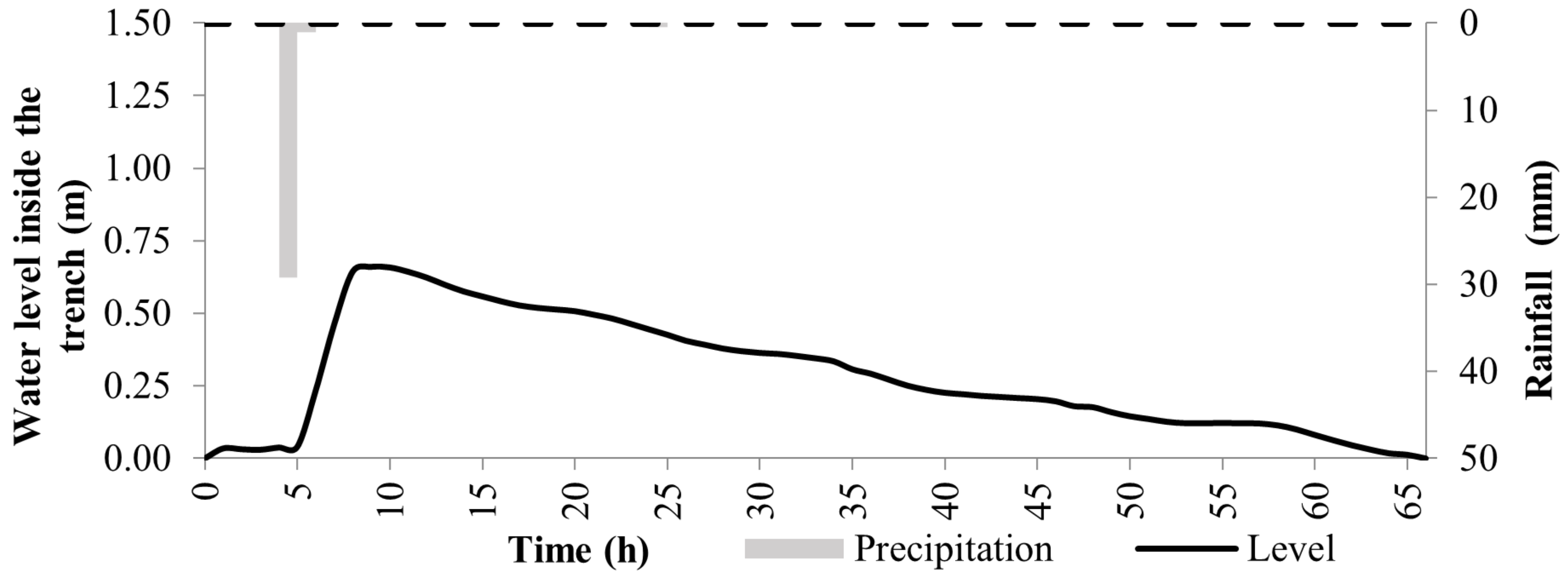
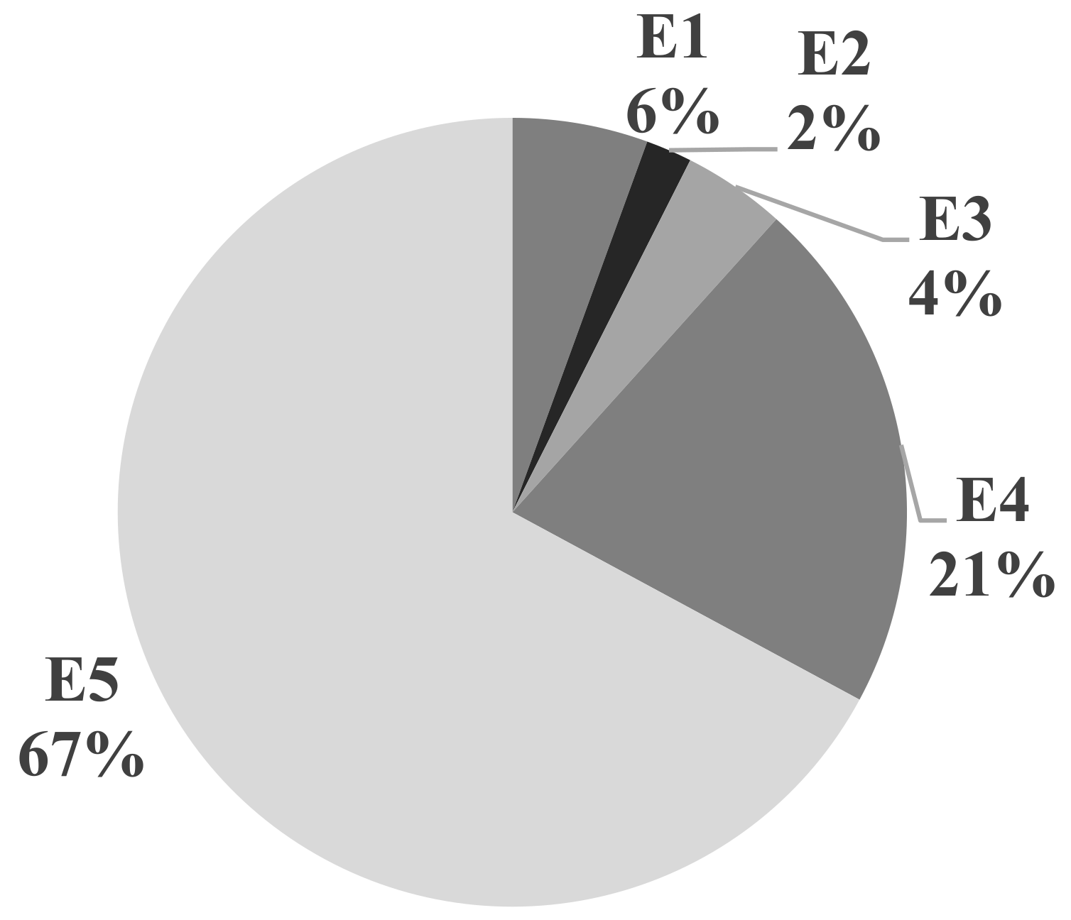
3.1. Infiltration Trench Monitoring and Analysis

Precipitation and water level data within the infiltration trench are shown in Figure 5. The continuous line represents the water level in the infiltration trench, and the dashed line represents the maximum depth (1.5 m). Water levels above this value express a system spillover. The events were selected through the analysis of recession curves with the observed precipitation.

For analysis of the infiltration trench, five events were highlighted. In each case, the infiltration system response time, the antecedent rainfall used to define initial soil conditions (I, II or III), the accumulated rainfall, the maximum height of the water level, the ascension and the recession time were verified. Figure 6 shows the trench behaviour in event 1 (E1) for the rainy season from 23 April to 25 April. The accumulated rainfall in the last five days before the studied moment was 1.2 mm, characterizing the initial soil condition as dry soil (I). The maximum rainfall of the highlighted event was 30.4 mm. The water level rose 0.66 m in 5 h and took 57 h to drain the volume of 1250.82 L completely. There was no system spillover during this event, and the entire captured volume was infiltrated. The average infiltration flow during the system recession period was 18.95 L/h.

Figure 7 shows the trench behaviour in event 2 (E2) for the rainy period from 29 April to 2 May. In this context, rainfall occurred in several blocks, causing oscillations in the system water level. The accumulated rainfall in the last five days before the event was 2.8 mm, corresponding to the initial condition of dry soil (I). The red circle with the numbers are the water level rise highlights of the event. The water level recession was affected by little rainfall, causing small fluctuations in the water level (See Figure 7, dashed red ellipses). The volume captured by the infiltration trench was 426.49 L. The latter was infiltrated in 46 h and represented an average infiltration flow of approximately 6.88 L/h.

Figure 8 shows the trench behaviour during event 3 (E3) for the rainy period from 2 May to 5 May. The red circle with the numbers are the water level rise highlights of the event. During the period, there were several blocks of rainfall, favouring the entry of water into the infiltration trench. The accumulated rainfall in the last five days before the event was 26.4 mm, corresponding to an initial condition of partially wetted soil (II). Event 3 (E3) was characterized by several moments of rising water level in the trench due to some blocks of precipitation. At first, the water level rose to 0.20 m in 5 h, due to the cumulative rainfall of 8.2 mm. After 2 h without rain, another 21.4 mm precipitation block was observed, and the water level rose to 0.50 m in 3 h. The third moment occurred due to a 15.6 mm precipitation block, which caused the water level to rise to 0.60 m in 8 h. In the fourth analysed moment, the water level of the trench rose to 0.62 m in 5 h due to a 7.4 mm precipitation block. In this event, the recession occurred in 49 h, meeting the recommended duration (72 h). It showed oscillations because of the precipitation that occurred during the process. The infiltration trench stored a volume of 950.55 L, which was thoroughly infiltrated at an average flow of 12.51 L/h.

Figure 9 shows the trench behaviour during event 4 (E4) for the rainy period from 27 May to 5 June 2017. In this event, several blocks of rainfall occurred. The accumulated rainfall in the last five days before the event was 36.6 mm, corresponding to initially wet soils (III). The wet initial condition resulted in slower water infiltration into the system. This occurs in situations where the drainage process is more prolonged, facilitating system leakages. In the first moment of this event, due to accumulated precipitation of 45.6 mm registered at hour 10, the trench level rose to 1.32 m. In the second moment, the water level dropped to 0.65 m in 19 h, even though there was an accumulated rainfall of 21.0 mm. The system recession movement was interrupted by another rainfall block of 34.4 mm in 6 h, causing the water level to rise again to 1.47 m. In an interval of 47 h with little rain, about 8.6 mm, the water level inside the infiltration trench dropped to 0.30 m. There was a 72.2 mm rainfall for 9 h after 90 h (see Figure 9, “5”), interrupting the recession process and raising the water level to 1.53 m, causing the system to overflow. From that moment, the water level inside the infiltration trench decreased to 0.10 m in 127 h. After 95 h, it was observed that the water level is sensitive to variations in the initial soil moisture conditions, with a lower infiltration rate in wet soil conditions.

Figure 10 shows the trench behaviour in event 5 (E5), for the rainy period from 6 June to 3 September. E5 was the longest event to be analyzed, with a series of precipitation blocks registered, making the system overflow several times. The total rainfall in the last five days before the event was 38.8 mm, corresponding to wet initial conditions (III).

The first analyzed moment occurred between 222 and 233 h when the accumulated precipitation was 45.2 mm, and the water level went from 0.60 to 1.46 m. During its decline, the water level reached 0.60 m in 192 h. During the process, the precipitation was 46 mm, distributed throughout the period. This precipitation disturbed the system infiltration process. The second analyzed moment occurred between 424 and 451 h when the water level went from 0.64 m to 1.51 m. At that moment, the system initial overflow happened, due to a 50.8 mm precipitation. The water level dropped to 0.96 m in 82 h and, during that process, rainfall was 21.4 mm. In the third studied moment, the water level in the trench went from 0.96 m to 1.58 m in 32 h, due to a 57 mm rainfall, representing the second overflow of this event. In the fourth moment, there were several overflows, in addition to some moments of level decrease. The total rainfall was 154.6 mm, and the trench water level reached 1.61 m. During this period, the soil was saturated, reducing the water infiltration velocity, and there was heavy rain in relatively short periods, causing several overflows. In the fifth moment, the accumulated rainfall was 29.2 mm in 239 h, and the water level dropped to 0.85 m. The moment was interrupted by another 117.8 mm rainfall block, which caused the trench water level to rise to 1.60 m in 43 h, consequently leading to water overflow. The sixth moment behaved similarly to the fourth, with many fluctuations in the water level and several overflows. The accumulated rainfall for this moment was 146.2 mm in 281 h. As a result, the water level ranged from 1.27 to 1.62 m. The seventh moment presented a water level reading failure. However, the analysis was not affected. The moment showed a recession that lasted 390 h, with accumulated rains of 40.2 mm during the process that prolonged the emptying time. The eighth moment exhibited a recession that lasted 160 h, with 32.4 mm of accumulated rain during the process. The ninth moment, on the other hand, exhibited a 78 h recession, with accumulated rainfall of 14.0 mm during the process. Event 5 (E5) stored 15120.86 L, corresponding to 67% of the infiltrated water volume. This volume was infiltrated at an average flow of 7.35 L/h.

During precipitation events, a decrease in the infiltration capacity of the soil supporting the infiltration trench is observed. When precipitation ceases, the process of recovering the soil’s infiltration capacity begins. In this context, depending on the infiltration trench geometry, the hydrodynamic and structural characteristics of the soil and the temporal dynamics of precipitation, the stored water drainage process can show great variability.

Emerson et al. [40] observed that, in a 5.7 m³ infiltration trench, the maximum emptying time was eight days, or approximately 192 h, during three years of monitoring. There were oscillations in the recession moments of the analyzed events, even without reading the precipitation on the device. These oscillations are observed in events E1, E2 and E3. Griffiths and Clausen [41] also observed this fact. These oscillations are attributed to the remaining water in the soil pores or in the infiltration system itself.

Figure 11 shows the percentage of infiltrated volume for each analyzed event. Event 5 (E5) was the one with the highest infiltration volume and the most prolonged duration, due to precipitations over short periods. Event 2 (E2), on the other hand, had the lowest percentage of infiltration due to the low volume precipitated in the period.

The average trench emptying time for this study was 6 days, the same as observed by Melo et al. [4] for this same structure. Drainage rate values in cm/h for events E1, E2, E3, E4.6, E5.5 and E5.7 are shown in

Table 2. Infiltration rate for each moment of recession of the events and the study’s general average. Rates in cm/h.

E1	E2	E3	E4.6	E5.5	E5.7
1.14	0.52	1.27	1.10	0.32	0.25

. According to Table 2, the highest infiltration rates occurred in events in which the soil condition was I and II, that is, dry soil and average humidity conditions. The lowest infiltration rates were found in E5, where the initial soil condition was III, i.e., wet soil. In addition, the soil infiltration rate in the trench for E2 was 0.52 cm/h, a value that differs from other values found under similar humidity conditions. Melo [42], studying this same structure, presented an average infiltration value of 0.83 cm/h. For these analyzed moments, the infiltration rate was 0.77 cm/h on average, with significant variability between events, as shown in Table 2.

Emerson et al. [40] found a reduction in the system infiltration rate from 10 cm/h to 0.10 cm/h over three years. They observed that the base of the structure had a more significant influence on the infiltration rate decrease due to clogging.

3.2. Sensitivity Analysis of the Model

Figure 12 shows the result of the model sensitivity analysis, performed for the event E1, for the value of the saturated hydraulic conductivity of the infiltration trench base and wall. The maximum level observed in E1 was 0.66 m, and the average infiltration velocity was 0.01 m/h. With the model simulation, the maximum calculated level in the trench was 0.38 m, that is, a difference of 0.28 m in level, from the observed to the calculated. The average infiltration velocity was 0.002 m/h, less than that observed. With the variation of the model infiltration capacity, the obtained results remained close to the values achieved with the optimal k found by the model until the moment of the maximum level. After that moment, there was a variation in the model infiltration velocity from 30%, 20%, 10%, 8%, 17% and 25% to −30%, −20%, −10%, 10%, 20 % and 30%, respectively.

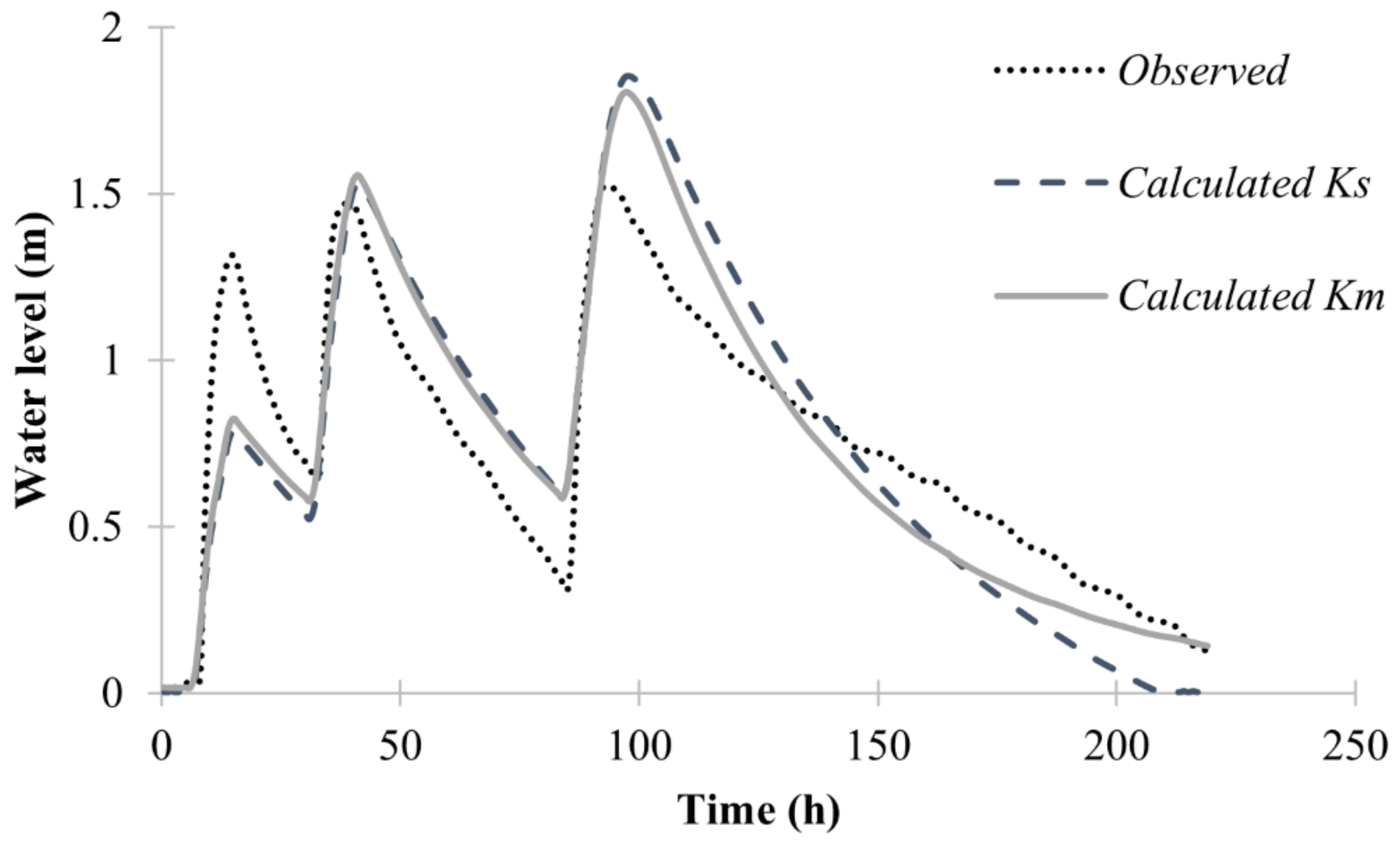
3.3. Modeled Data of the Infiltration Trench

For the analyzed period, the simulation was performed with the Puls method, and calculated data consistency was checked with those observed in the field, the simulations with the unique k for wall and base represented by Ks, Km representing the simulations with different values of k for the wall and base. Figure 13 shows the comparison of the simulated and observed water levels in the infiltration trench. The simulations and observed data show the same behaviour for the period, with increasing and decreasing levels, showing the same trend throughout the analysis. The level curves found by the model are smoother and have smaller magnitudes compared to the observed data. The R² for this analysis was 0.80 for the simulation with Km and 0.68 for the simulation with Ks.

Figure 14 shows the E2 simulation with the Puls method. There is a comparison between the data observed in the field and those calculated by the model. The simulation by Puls obtained a water level peak of 0.22 m, with a difference of 0.02 m from that observed. From the maximum height simulated, the level dropped to 0.05 m in 50 h. The optimization for this event showed an optimal infiltration capacity of 0.0060 m/h and 0.0001 m/h for the walls and the base, respectively. The infiltration capacity for simulation with a single variable was 0.0014 m/h. The R² for this analysis was 0.86 for Km and 0.84 for Ks.

Figure 15 shows the simulation with the Puls model for the event E3. The simulated period was from 2 to 5 May 2017. The simulated event obtained an R² of 0.89, a DR of 1.43 and a CRM of −3.12 × 10⁻¹⁴ for Km and an R² of 0.86, a DR of 1.38 and a CRM of −2.26 × 10⁻⁷ for Ks. The maximum height of the water level was 0.6 m, and it took 28 h to reach that level. The system’s recession time equalled 50 h. The optimal infiltration capacity of the method generated k_b and k_w of 0.0001 m/h and 0.004 m/h, respectively. With the same infiltration capacity for the base and the walls, we obtained an optimum value of 0.0018 m/h. The maximum water level observed for the event was 0.62 m, 0.02 m above the simulated.

Figure 16 shows the simulation with the Puls model for the event E4. The simulated period was from 27 May to 5 June 2017. The simulated data followed the variation of the water levels inside the infiltration trench. In some situations, such as in the first and third peaks of the water level, the observed and calculated data had very different peak values. The last variation of the water level in the simulation occurred after 123 h and reached 0.14 m for the simulation with two variables (Km) and 0 m for the simulation with one variable (Ks). Note that the level data at the second and third peaks were higher than those simulated. The R² of the simulation was 0.84 for Km and 0.82 for Ks.

As seen in Figure 13, Figure 14, Figure 15 and Figure 16, small precipitation volumes can generate discontinuity in the recession curve, causing small increases in the volume stored. However, such a feature may be common in infiltration techniques inserted in tropical climates, where precipitation can be very frequent with short dry periods between rainfall events, mostly during the wet periods. In these situations, the model presents difficulties in representing the observed data. Furthermore, by assuming constant hydraulic conductivity, the model disregards variations in the degree of soil saturation around the infiltration trench.

Table 3. Infiltration capacity values (m/h) in the base (k_b) and in the wall (k_w) of the Km simulation and the infiltration capacity k (m/h) for the Ks simulation.

Simulation	Km		Ks
	kb	kw	k
Event 2	1.26 × 10−4	5.99 × 10−3	1.42 × 10−3
Event 3	1.25 × 10−4	4.09 × 10−3	1.84 × 10−3
Event 4	1.25 × 10−4	4.05 × 10−3	2.63 × 10−3
Complete event	1.27 × 10−4	8.35 × 10−3	4.98 × 10−3
Average values	1.25 × 10−4	5.62 × 10−3	2.72 × 10−3
Standard deviation	1.05 × 10−6	2.03 × 10−3	1.59 × 10−3
Coefficient of variation	8.34 × 10−3	3.62 × 10−1	5.85 × 10−1

presents the infiltration capacity values obtained in each event and for the entire simulated period. In addition, the same table shows the average values, the standard deviation and the coefficient of variation of the exposed data. In Table 3, it can be verified that infiltration capacity (k_b) values show little variation between simulations. The values obtained from the standard deviation and the variation coefficient, respectively, were 1.05 × 10⁻⁶ and 8.34 × 10⁻³. For the wall, the infiltration capacity (k_w) values are the ones that vary the most, with the lowest value found in event E4, and the highest in the simulation of the complete event. The values of standard deviation and the coefficient of variation, respectively, were 2.03 × 10⁻³ and 3.62 × 10⁻¹. The infiltration capacity k, on the other hand, showed a variation greater than k_b and less than k_w, for which the value of the standard deviation between simulations was 1.59 × 10⁻³. The greatest infiltration capacity for this condition was obtained for the simulation of the complete event.

It can be observed in Table 3 that the infiltration capacity of the wall (k_w) is greater than that of the base (k_b). This occurs due to the clogging of the base by sedimentation of fine particles at the bottom of the system. Base clogging occurs naturally, and older structures are more prone to these situations. The studied infiltration trench has been built for 7 years, and naturally the base has a significant degree of clogging. Overall, the contribution of the horizontal flow (on the wall) becomes more important for these structures with time.

Table 4. Coefficient of determination (R²), deviation ratio (DR) and coefficient of residual mass (CRM).

Simulation	Km			Ks
	R2	DR	CRM	R2	DR	CRM
Event 2	0.86	1.86	3.24 × 10−7	0.84	1.45	1.27 × 10−6
Event 3	0.89	1.43	−3.12 × 10−14	0.86	1.38	−2.26 × 10−7
Event 4	0.84	0.69	−1.32 × 10−9	0.82	0.56	−4.23 × 10−9
Complete event	0.80	2.79	5.96 × 10−7	0.68	1.93	4.35 × 10−8
Average	0.85	1.69	2.31 × 10−7	0.80	1.33	2.70 × 10−7

presents a summary of the three statistical parameters of this study. These parameters characterize the quality of the fits obtained with the Puls method.

It is observed that the determination coefficient obtained the greatest adjustment in event E3 of 0.89, while the simulation of the complete event obtained the lowest adjustment of 0.80 for the simulation (Km) with two variables (k_w and k_b). As for the simulation (Ks) with one variable, the highest value of the coefficient of determination was 0.86 in event 3 and the lowest was 0.68 (incomplete event). The deviation ratio describes the ratio between the dispersion of the calculated values and the corresponding theoretical model, with values that deviate from the reference. The residual mass coefficient in event E3 for the simulation with two variables performed better, getting closer to the reference value, while the residual mass coefficient in Ks had the best performance for event E4.

For Barbassa et al. [43], simulations using the Puls method were distant from the observations for water level lower than 0.2 m. This can be explained by the clogging level at the base of the system and by a small hydraulic load that this water level exerts on the soil. However, in event E2 of this study, where the observed data were close to the level mentioned by Barbassa et al. [43], the simulation obtained a good determination coefficient, with the infiltration of the system wall compensating for the low infiltration at the base. The average R² concerning the structure behaviour relative to the water level inside the trench was 0.85 and 0.80, thus obtaining a good fit of the observed data. In studies by Tecedor et al. [29], the average R² found in the system by simulation with the Puls method was 0.71.

In this context, future research may evaluate the use of models based on the Richards equation to simulate the dynamics of the trench water level, as used in [44,45]. In addition, the results presented in this article may be due to a strong influence of the heterogeneity of the subsoil [46], the sensitivity of the hydrodynamic parameters of the soil [47], the evolution over time of the soil trench clogging processes [48], as well as the seasonality of infiltration processes as a function of climatic conditions [49], which can be evaluated in the future.

4. Conclusions

Continuous monitoring of the infiltration trench is essential to understand the functioning of infiltration trenches in order to promote their use as a compensatory technique in urban areas. It is necessary to analyze and quantify infiltration trench performance at several periods, making it possible to assess performance over time. The infiltration trench showed satisfactory results, with high water infiltration rates during the monitoring period, even with system overflows. These overflows were due to the very high rainfall typical of the studied region (tropical climate), with high precipitation events in short periods.

The need for maintenance of this type of structure was observed during this work. The loss of efficiency in the base’s infiltration capacity is caused by the clogging process, where fine particles deposit at the bottom of the system. Clogging at the base of the structure occurs naturally and can be a disadvantage of these compensatory techniques. As the study’s infiltration trench was built in 2014, the decrease in bottom drainage is natural. This fact is observed in this work, where the infiltration capacity of the base is lower than that of the wall. The infiltration trench has a water storage volume of 2227.50 L, which is quite sizeable and allows the storage and infiltration of a large volume of stormwater. The analyzed events presented an average emptying time of 6 days. The system overflowed several times, mainly during the months of higher precipitation rates. The infiltration trench has achieved its goal of decreasing effective precipitation and decreasing the volume of water to collect and route to sewer systems.

We also used the Puls method and confirmed its adequacy for the modelling of such structures. Verifying the adequacy of the Puls method is relevant to the project’s viability analysis of the studied infiltration trench. The R² values ranged from 0.68 to 0.89 and were higher at the scale of the event than at the scale of larger periods (with a collection of several events). In the longer events, different pulses of rain occurred at various times, generating discontinuity in the recession curve, causing small increases in the volume stored. In these situations, the model presents difficulties in representing the observed data. Furthermore, by assuming constant hydraulic conductivity, the model disregards variations in the degree of soil saturation and related impacts on hydraulic conductivity. However, the fits proved very good, apart from a few exceptions. Our results proved relevant for the understanding of the functioning of the studied trench and the quantification of its significant impact on the water budget.

References

1. Hamel, P.; Daly, E.; Fletcher, T.D. Source-control stormwater management for mitigating the impacts of urbanisation on baseflow: A review. J. Hydrol. 2013, 485, 201–211. [Google Scholar] [CrossRef]
2. Melo, T.A.T.; Coutinho, A.P.; Cabral, J.J.S.P.; Antonino, A.C.D.; Cirilo, J.A. Jardim de Chuva: Sistema de Biorretenção Para o Manejo Das Águas Pluviais Urbanas. Ambiente Construído Porto Alegre 2014, 14, 147–165. [Google Scholar] [CrossRef]
3. Li, J.Q.; Xiang, L.L.; Che, W.; Ge, R.L. Design and Hydrologic Estimation Method of Multi-Purpose Rain Garden: Beijing Case Study. In Low Impact Development for Urban Ecosystem and Habitat Protection, Proceedings of the International Low Impact Development Conference 2008, Seattle, WA, USA, 16–19 November 2008; American Society of Civil Engineers: Reston, VA, USA, 2009; Volume 67, pp. 1–10. [Google Scholar]
4. Melo, T.; Coutinho, A.P.; Dos Santos, J.B.F.; Cabral, J.J.D.S.P.; Antonino, A.C.D.; Lassabatere, L. Trincheira de Infiltração Como Técnica Compensatória No Manejo Das Águas Pluviais Urbanas. Ambiente Construído 2016, 16, 53–72. [Google Scholar] [CrossRef] [Green Version]
5. Coutinho, A.P.; Lassabatere, L.; Winiarski, T.; Cabral, J.J.S.P.; Antonino, A.C.D.; Angulo-Jaramillo, R. Vadose Zone Heterogeneity Effect on Unsaturated Water Flow Modeling at Meso-Scale. J. Water Resour. Prot. 2015, 7, 353–368. [Google Scholar] [CrossRef] [Green Version]
6. El-Mufleh, A.; Béchet, B.; Ruban, V.; Legret, M.; Clozel, B.; Barraud, S.; Gonzalez-Merchan, C.; Bedell, J.-P.; Delolme, C. Review on Physical and Chemical Characterizations of Contaminated Sediments from Urban Stormwater Infiltration Basins within the Framework of the French Observatory for Urban Hydrology (SOERE URBIS). Environ. Sci. Pollut. Res. 2014, 21, 5329–5346. [Google Scholar] [CrossRef]
7. Rowe, A.A.; Borst, M.; O’Connor, T.P. Pervious Pavement System Evaluation. In Proceedings of the World Environmental and Water Resources Congress 2009, Great River, Kansas City, MS, USA, 17–21 May 2009. [Google Scholar]
8. Coutinho, A.P.; Lassabatere, L.; Montenegro, S.; Antonino, A.C.D.; Angulo-Jaramillo, R.; Cabral, J.J.S.P. Hydraulic Characterization and Hydrological Behaviour of a Pilot Permeable Pavement in an Urban Centre, Brazil. Hydrol. Process. 2016, 30, 4242–4254. [Google Scholar] [CrossRef]
9. Jabur, A.S.; Dornelles, F.; Silveira, A.L.L.; Goldenfum, J.A.; Okawa, C.M.P.; Gasparini, R.L. Determination of the Infiltration Capacity of Permeable Pavements. Rev. Bras. Recur. Hídricos 2015, 20, 937–945. [Google Scholar]
10. Lucas, A.H.; Sobrinha, L.A.; Moruzzi, R.B.; Barbassa, A.P. Evaluation of Best Management Practices’ Construction and Operation: The Fine Particles Transportation, the Infiltration Capacity, the Soil Infiltration Loading Rate and the Geotextile Permeability. Eng. Sanit. E Ambient. 2015, 20, 17–28. [Google Scholar] [CrossRef] [Green Version]
11. Nascimento, N.O.; Baptista, M.B. Técnicas Compensatórias em Águas Pluviais. In Manejo Águas Pluviais; ABES: Rio de Janeiro, RJ, Brazil, 2009; pp. 148–197. Available online: http://www.finep.gov.br/images/apoio-e-financiamento/historico-de-programas/prosab/prosab5_tema_4.pdf (accessed on 15 June 2021).
12. Fletcher, T.D.; Shuster, W.; Hunt, W.F.; Ashley, R.; Butler, D.; Arthur, S.; Trowsdale, S.; Barraud, S.; Semadeni-Davies, A.; Bertrand-Krajewski, J.-L.; et al. SUDS, LID, BMPs, WSUD and More—The Evolution and Application of Terminology Surrounding Urban Drainage. Urban Water J. 2015, 12, 525–542. [Google Scholar] [CrossRef]
13. Askarizadeh, A.; Rippy, M.A.; Fletcher, T.D.; Feldman, D.L.; Peng, J.; Bowler, P.; Mehring, A.S.; Winfrey, B.K.; Vrugt, J.A.; AghaKouchak, A.; et al. From Rain Tanks to Catchments: Use of Low-Impact Development to Address Hydrologic Symptoms of the Urban Stream Syndrome. Environ. Sci. Technol. 2015, 49, 11264–11280. [Google Scholar] [CrossRef] [Green Version]
14. Houle, J.J.; Roseen, R.M.; Ballestero, T.P.; Puls, T.A.; Sherrard, J., Jr. Comparison of Maintenance Cost, Labor Demands, and System Performance for LID and Conventional Stormwater Management. J. Environ. Eng. 2013, 139, 932–938. [Google Scholar] [CrossRef]
15. Ahiablame, L.M.; Engel, B.A.; Chaubey, I. Effectiveness of Low Impact Development Practices in Two Urbanized Watersheds: Retrofitting with Rain Barrel/Cistern and Porous Pavement. J. Environ. Manag. 2013, 119, 151–161. [Google Scholar] [CrossRef] [PubMed]
16. Jia, H.; Wang, Z.; Zhen, X.; Clar, M.; Yu, S.L. China’s Sponge City Construction: A Discussion on Technical Approaches. Front. Environ. Sci. Eng. 2017, 11, 18. [Google Scholar] [CrossRef]
17. Vincent, S.U. Sustainable Drainage Systems as Ecosystem Services Case Study: Urban Catchment in Montevideo, Uruguay; UNESCO-IHE Institute for Water Education: Delft, The Netherlands, 2013. [Google Scholar]
18. Thorne, C.R.; Lawson, E.C.; Ozawa, C.; Hamlin, S.L.; Smith, L.A. Overcoming Uncertainty and Barriers to Adoption of Blue-Green Infrastructure for Urban Flood Risk Management. J. Flood Risk Manag. 2018, 11, S960–S972. [Google Scholar] [CrossRef]
19. Nguyen, T.T.; Ngo, H.H.; Guo, W.; Wang, X.C.; Ren, N.; Li, G.; Ding, J.; Liang, H. Implementation of a Specific Urban Water Management—Sponge City. Sci. Total Environ. 2019, 652, 147–162. [Google Scholar] [CrossRef]
20. Zevenbergen, C.; Fu, D.; Pathirana, A. Transitioning to Sponge Cities: Challenges and Opportunities to Address Urban Water Problems in China. Water 2018, 10, 1230. [Google Scholar] [CrossRef] [Green Version]
21. Reis, R.P.A.; Ilha, M.S.D.O.; Teixeira, P.D.C. Sistemas Prediais de Infiltração de Água de Chuva: Aplicações, Limitações e Perspectivas. REEC—Rev. Eletrôn. Eng. Civ. 2013, 7, 55–67. [Google Scholar] [CrossRef] [Green Version]
22. Li, Y.; Buchberger, S.G.; Sansalone, J.J. Variably Saturated Flow in Storm-Water Partial Exfiltration Trench. J. Environ. Eng. 1999, 125, 556–565. [Google Scholar] [CrossRef]
23. Ohnuma, A.A.; Da Silva, L.P.; Mendiondo, E.M. Input Flows for the Infiltration Trench Household. Cienc. Eng. Sci. Eng. J. 2015, 24, 89–98. [Google Scholar] [CrossRef] [Green Version]
24. Locatelli, L.; Mark, O.; Mikkelsen, P.S.; Arnbjerg-Nielsen, K.; Wong, T.; Binning, P.J. Determining the Extent of Groundwater Interference on the Performance of Infiltration Trenches. J. Hydrol. 2015, 529, 1360–1372. [Google Scholar] [CrossRef] [Green Version]
25. Duchêne, M.; McBean, E.A.; Thomson, N.R. Modeling of Infiltration from Trenches for Storm-Water Control. J. Water Resour. Plan. Manag. 1994, 120, 276–293. [Google Scholar] [CrossRef]
26. SWMMWW. Stormwater Management Manual for Western Washington. Available online: https://ecology.wa.gov/Regulations-Permits/Guidance-technical-assistance/Stormwater-permittee-guidance-resources/Stormwater-manuals (accessed on 8 June 2017).
27. Lucas, A.H.; Barbassa, A.P.; Moruzzi, R.B. Modelagem de Um Sistema Filtro-Vala-Trincheira de Infiltração Pelo Método de Puls Adaptado Para Calibração de Parâmetros. Rev. Bras. Recur. Hídricos 2013, 18, 135–236. [Google Scholar] [CrossRef]
28. Zhang, K.; Chui, T.F.M. A Review on Implementing Infiltration-Based Green Infrastructure in Shallow Groundwater Environments: Challenges, Approaches, and Progress. J. Hydrol. 2019, 579, 124089. [Google Scholar] [CrossRef]
29. Tecedor, N. Monitoramento e Modelagem Hidrológica de Plano de Infiltração Construído em Escala Real. Master’s Thesis, Universidade Federal de São Carlos, São Carlos, Brazil, 2014. [Google Scholar]
30. Bezerra, P.H.L. Dinâmica da Água em Trincheira de Infiltração em Lote Urbano. Master’s Thesis, Universidade Federal de Pernambuco, Recife, Brazil, 2018. [Google Scholar]
31. Da Silva, S.R.; de Sousa Araújo, G.R. Algoritmo Para Determinação da Equação de Chuvas Intensas (Algorithm to Determine the Equation of Intense Rain). Rev. Bras. Geogr. Fís. 2013, 6, 1371–1383. [Google Scholar] [CrossRef] [Green Version]
32. APAC. Agência Pernambucana de Águas e Clima. Available online: http://old.apac.pe.gov.br/meteorologia/monitoramento-pluvio.php (accessed on 15 August 2018).
33. Silva, F.C. Manual de Análises Químicas de Solos, Plantas e Fertilizantes; Embrapa Informação Tecnológica: Brasília, Brazil, 2009. [Google Scholar]
34. Dos Santos, J.B.F. Monitoramento e Simulação Hidráulica de Uma Trincheira de Infiltração. Master’s Thesis, Universidade Federal de Pernambuco, Recife, Brazil, 2014. [Google Scholar]
35. McCuen, R.H. Hydrologic Analysis and Design, 4th ed.; Pearson: London, UK, 2016; ISBN 978-0-13-431312-2. [Google Scholar]
36. Tucci, C.E. Modelos Hidrológicos; Editora da UFRGS: Porto Alegre, Brazil, 2005; ISBN 978-85-7025-823-6. [Google Scholar]
37. Kuo, C.Y.; Zhu, J.L.; Dollard, L.A. Infiltration Trenches for Urban Runoff Control. In Hydraulic Engineering; ASCE: Reston, VA, USA, 1989; pp. 1029–1034. [Google Scholar]
38. Ferreira, L.T.L.M.; das Neves, M.G.F.P.; de Souza, V.C.B. Puls Method for Events Simulation in a Lot Scale Bioretention Device. RBRH 2019, 24, e36. [Google Scholar] [CrossRef] [Green Version]
39. Baptista, M.; Nascimento, N.; Barraud, S. Técnicas Compensatórias Em Drenagem Urbana [Compensatory Techniques for Urban Drainage]; ABRH: Porto Alegre, Brazil, 2015. [Google Scholar]
40. Emerson, C.H.; Wadzuk, B.M.; Traver, R.G. Hydraulic Evolution and Total Suspended Solids Capture of an Infiltration Trench. Hydrol. Process. 2010, 24, 1008–1014. [Google Scholar] [CrossRef]
41. Griffiths, G.A.; Clausen, B. Streamflow Recession in Basins with Multiple Water Storages. J. Hydrol. 1997, 190, 60–74. [Google Scholar] [CrossRef]
42. De Melo, T.D.A.T. Avaliação Hidrodinâmica de Trincheira de Infiltração No Manejo Das Águas Pluviais Urbanas. Ph.D. Thesis, Universidade Federal de Pernambuco, Recife, Brazil, 2015. [Google Scholar]
43. Barbassa, A.P.; Angelini Sobrinha, L.; Moruzzi, R.B. Poço de Infiltração Para Controle de Enchentes Na Fonte: Avaliação Das Condições de Operação e Manutenção. Ambiente Construído Porto Alegre 2014, 14, 91–107. [Google Scholar] [CrossRef] [Green Version]
44. Brunetti, G.; Šimůnek, J.; Piro, P. A comprehensive analysis of the variably saturated hydraulic behavior of a green roof in a mediterranean climate. Vadose Zone J. 2016, 15, vzj2016.04.0032. [Google Scholar] [CrossRef] [Green Version]
45. Farahi, G.; Khodashenas, S.R.; Alizadeh, A.; Ziaei, A.N. New model for simulating hydraulic performance of an infiltration trench with finite-volume one-dimensional Richards’ equation. J. Irrig. Drain. Eng. 2017, 143, 04017025. [Google Scholar] [CrossRef]
46. D’Aniello, A.; Cimorelli, L.; Cozzolino, L.; Pianese, D. The effect of geological heterogeneity and groundwater table depth on the hydraulic performance of stormwater infiltration facilities. Water Resour. Manag. 2019, 33, 1147–1166. [Google Scholar] [CrossRef]
47. Brunetti, G.; Šimůnek, J.; Turco, M.; Piro, P. On the use of global sensitivity analysis for the numerical analysis of permeable pavements. Urban Water J. 2018, 15, 269–275. [Google Scholar] [CrossRef] [Green Version]
48. Freni, G.; Mannina, G. Long term efficiency analysis of infiltration trenches subjected to clogging. In New Trends in Urban Drainage Modelling; Springer: Cham, Switzerland, 2018; pp. 181–187. [Google Scholar]
49. Ebrahimian, A.; Wadzuk, B.; Sokolovskaya, N. Temporal Variation of Infiltration in Green Infrastructure. In AGU Fall Meeting Abstracts; American Geophysical Union: Washington, DC, USA, 2019; p. H44E-08. [Google Scholar]
Figure 1. Infiltration trench location in the city of Recife, PE.
Water 14 00513 g001
Figure 2. Infiltration trench and monitoring equipment: infiltration trench (1), piezometer (2 and 3), triangular spillway (4), passage box (5) and rain gauge (6).
Water 14 00513 g002
Figure 3. Infiltration trench perspective. (Source: [4]).
Water 14 00513 g003
Figure 4. Inlet box triangular spillway.
Water 14 00513 g004
Figure 5. Continuous monitoring of precipitation and water level in the infiltration trench for the study period.
Water 14 00513 g005
Figure 6. Infiltration trench event 1 (E1) from 23 April to 25 April 2017.
Water 14 00513 g006
Figure 7. Infiltration trench event 2 (E2) from 29 April to 2 May from 2017. The different numbers correspond to the different parts of the curves that are discussed in the text.
Water 14 00513 g007
Figure 8. Infiltration trench event 3 (E3) from 2 May to 5 May 2017. The different numbers correspond to the different parts of the curves that are discussed in the text.
Water 14 00513 g008
Figure 9. Infiltration trench event 4 (E4) from 27 May to 5 June 2017. The different numbers correspond to the different parts of the curves that are discussed in the text.
Water 14 00513 g009
Figure 10. Infiltration trench event 5 (E5) from 6 June to 3 September from 2017. The different numbers correspond to the different parts of the curves that are discussed in the text.
Water 14 00513 g010
Figure 11. Percentage of the infiltrated volume per analyzed event.
Water 14 00513 g011
Figure 12. Model sensitivity analysis with regards to the value of the saturated conductivity, bottom and wall of the infiltration trench.
Water 14 00513 g012
Figure 13. Simulation of the entire monitored period.
Water 14 00513 g013
Figure 14. Event E2 simulation.
Water 14 00513 g014
Figure 15. Event E3 simulation.
Water 14 00513 g015
Figure 16. Event E4 simulation.
Water 14 00513 g016