Linking Urban Floods to Citizen Science and Low Impact Development in Poorly Gauged Basins under Climate Changes for Dynamic Resilience Evaluation

Abstract

Cities must develop actions that reduce flood risk in the face of extreme rainfall events. In this study, the dynamic resilience of the Gregorio catchment (São Carlos, Brazil) was assessed. The catchment lacks environmental monitoring and suffers from recurrent floods. The resilience curves were made considering the water depth in the drainage system as the performance index, obtained by simulations with SWMM and HEC-RAS. The calibration of the flood extension was performed using citizen science data. The contribution to increasing the dynamic resilience by implementing decentralized low impact development (LID) practices was also evaluated. For this purpose, bioretention cells were added to the SWMM simulations. The resilience curves were then calculated for the current and future climate scenario, with and without LID, for return periods of 5, 10, 50, and 100 years and duration of 30, 60, and 120 min. Intensity–duration–frequency curves (IDFs) updated by the regional climate model MIROC5 for 2050 and 2100 were used. The results showed a significant improvement in the system’s resilience for light storms and the current period due to LID practice interventions. Efficiencies were reduced for moderate and heavy storms with no significant drops in floodwater depth and resilience regardless of the scenario.

1. Introduction

Historically, cities have been affected by extreme rainfall events and their consequences such as floods and landslides [1,2,3,4]. Poor planning and management of the urban space contributes to increasing flood risk for the population due to the housing settlement in steep or floodplain areas and excessive impervious areas and consequently higher runoff generation [5,6,7]. In developing countries, the housing deficit further increases the occupation of hazardous areas by socially vulnerable populations. Additionally, the pattern of urban occupation and creation of cities has been around rivers due to the need for access to water resources; in many cities, the traditional commercial center is located near floodplain areas [8,9].

Climate change aggravates this risk scenario by increasing the probability of extreme events and their intensities [10,11,12]. Studies in different regions worldwide show a trend of higher occurrence of storm events, even when there is a decrease in the total rainfall volume in the wet season [13,14,15]. This trend is also observed in Brazil’s regional climate models (RCM) developed with climate change [16,17]. A total reduction in the rainfall volume in southeastern Brazil has been observed with an increase in extreme events. These results were reaffirmed, including more pessimistic forecasts, in the IPCC’s Sixth Assessment Report, working group 1: the physical science basis (AR6) [18].

As a guideline for disaster risk management caused by extreme events, the United Nations Office on Disaster Risk Reduction (UNDRR) released the Sendai report in 2015 [19], presenting increased resilience as the ultimate goal to be pursued by decision makers. This report presents the importance of taking risk management actions from a science–policy interface for risk-oriented and evidence-based decision making [20], (pp. 3–5, [21]), (pp. 51–68, [22]).

This report defines resilience as “the ability of a system, community or society exposed to hazards to resist, absorb, accommodate, adapt to, transform and recover from the effects of a hazard in a timely and efficient manner, including through the preservation and restoration of its essential basic structures and functions through risk management.” Several actions have been proposed to increase the resilience of cities to flood events, considering the different temporal components of risk management actions (anticipation, prevention, mitigation, preparedness, response, and recovery [19,23]). Furthermore, actions can be classified as structural, measures, or non-structural, instruments [24].

Structural prevention and mitigation measures are commonly used by cities with the main application of centralized grey infrastructures such as detention basins and rainwater reservoirs [25,26,27]. However, in recent years, the application of green infrastructure measures, also known as low impact development (LID) practices, has grown due to their complementary benefits for the hydrological cycle, diffuse pollution control, and the catchment life cycle [28]. According to the 2014 report of the C40 group, drainage solutions with LID ranked third among the most performed actions by the group’s cities [29].

Due to the central importance of resilience in the risk-oriented and evidence-based decision-making process, several studies aimed to define its indicators. In [30,31], the authors criticized the application of static resilience indicators since they do not allow a good representation of the event cycle after stress and consequently the evaluation of the temporal components of risk management actions. Thus, the authors proposed a space-time dynamic resilience measure (STDRM). For this measure, resilience is presented as the loss of system performance (e.g., physical, social, economic, health, etc.), which can be calculated as the integral of the curve representing the system performance level between the beginning of the disruptive event and the end of the system’s recovery. Over time and space, the different performance metrics can be further normalized and combined into a single resilience curve.

The system’s performance can be quantified through computational modelling, allowing the evaluation and comparison of different intervention scenarios [32,33]. In the case of resilience to flood events, a commonly used metric for the physical system is the water depth reached by the flood and its horizontal extent in the affected area. To this end, hydrological, hydraulic, and hydrodynamic models must be used [34,35]. However, limited hydrological data availability can hinder urban flood modelling [36].

In order to simulate both pluvial and fluvial floods happening simultaneously in urban catchments, coupled hydrological and hydrodynamical modelling have been increasingly used. One common configuration is to use HEC-HMS for hydrological modelling and HEC-RAS for the hydrodynamic 2D process, obtaining the flood extensions and flood depths for different scenarios [37,38,39]. This configuration has been used in ungauged or poorly gauged basins with a high application in India. Nevertheless, there are some limitations in using HEC-HMS for hydrological modelling: it does not allow simulation of the effect of LID practices and it does not account water quality assessment.

To overcome these issues, it is possible to use an alternative configuration such as coupling SWMM and SWAT for hydrological modelling with HEC-RAS. SWMM and SWAT models allow us to incorporate different types of LID practices in the catchment, e.g., rain gardens, green roof, porous pavement, etc. [40,41]. The SWMM model has been widely used for urban catchments [42,43,44] while the SWAT model has been more applied in large areas [45].

In [46], the authors successfully used SWMM to assess the impact of climate change on an small urban catchment in Athens, Greece by updating IDF curves due to climate change and demonstrated that under the non-stationarity projections of climate, the percent change in future rainfall intensity could vary immensely and showed the potential of a systematic assessment of flood mitigation scenarios by using climate projections, bias correction methods, and temporal downscaling associated with hydraulic models. In the same sense, [47] found that climate change would reduce total rainfall in Tehran but with an increase in heavy storms. Therefore, the authors evaluated these non-stationary effects in the urban hydrology by using SWMM and proposed different intervention scenarios with LID practices to maintain the urban resilience. SWMM was also used in [48] to assess the impact of climate change on urban hydrology and their impacts on combined-sewer overflow occurrences in city of Toledo, Ohio, obtaining an increase of 12–18% for future scenarios. Additionally, the simulation showed that rainwater harvesting implementation in half of the buildings could mitigate the effects of future climates.

Despite the contribution of these studies to evaluate mitigation measures to climate change by LID practices, they only performed hydrological modelling and did not provide information about flood extent and depth. For this purpose, coupling SWMM with HEC-RAS can be an alternative [49].

For a good representation of the area by coupled hydrological and hydrodynamic modelling, it is necessary to calibrate and validate the models with observed data with different severities and probabilities of occurrence. However, in the case of developing countries, it is common for urban catchments to be poorly gauged, lacking observed data with suitable temporal and spatial discretization [39,50,51,52]. To overcome this problem, new studies have used citizen science data—the involvement of citizens in collecting data and knowledge for scientific research [53] and historical records—and social data such as photos, footage from security cameras, newspapers, and population memory to extract records of depths and flows of flood events [54,55,56], showing a clear potential for using data collected by citizens to complement traditional monitoring data for flood model development and validation, especially at ungauged or poorly gauged catchments. Data reported from citizens also benefit from being spatial and can be compared to other spatial datasets [57]. Case studies have shown that even when the amount of data is not so expressive, they can still provide an effective form of model validation [58]. Additionally, [59] showed that regionalization methods and optimization techniques [60] were helpful for LID simulation to overcome the lack of hydrological and stormwater quality data.

The state of São Paulo (SP) in the city of São Carlos in Brazil has had recurrent cases of flooding over the years, with critical flooded areas in its main commercial center [61,62]. However, due to traditional cultural aspects, there is a permanence of commercial establishments in the risk area, making an eviction of the area unfeasible [62]. Therefore, it is necessary to develop risk management actions to reduce peak flows and flooding water depths in critical areas, reducing the damage generated.

This study aimed to explore the effect of different climate scenarios, combined with the implementation of LID practices as a structural measure of risk management, on the extent and depth of flooding in the center of São Carlos. To this end, SWMM and HEC-RAS software were used for hydrological and hydrodynamic modelling of the catchment. Due to the absence of observed monitored data as the catchment is poorly gauged, records extracted from population memory and register (citizen science) were used to calibrate and validate the models. Finally, the different scenarios were compared for their effect on the catchment resilience using the STDRM approach.

2. Case Study and Datasets

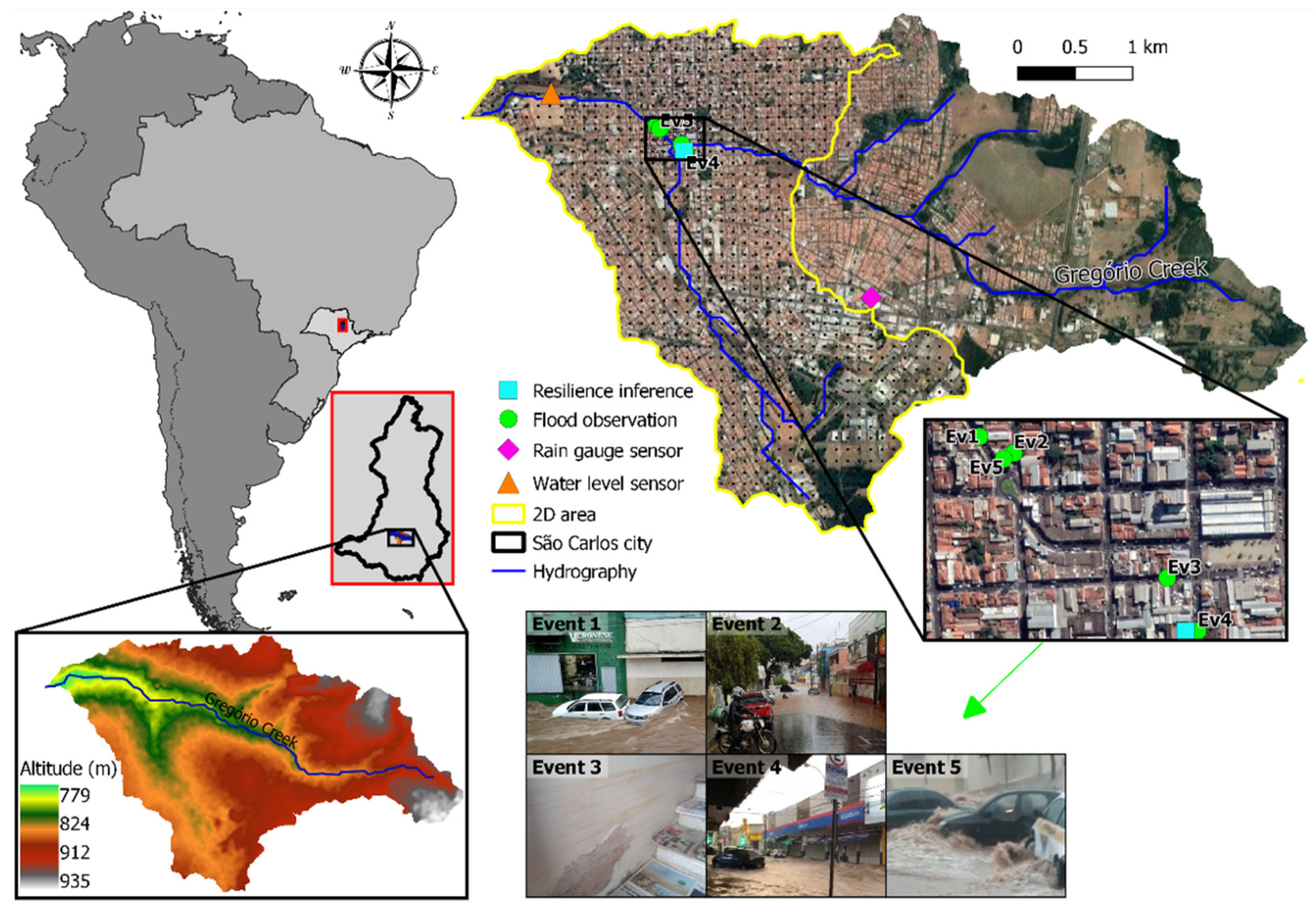
2.1. Gregorio Creek and Its Flood History

The case study was the Gregorio catchment located in the city of São Carlos, state of São Paulo, Brazil (Figure 1, zoom map on the left). The total area of the municipality of São Carlos is about 1136.91 km². The city’s population density is about 194.53 inhabitants/km², and the entire population is estimated as 249,415 inhabitants [63]. The average altitude is 856 m a.s.l. and the soil is highly permeable. As for its climatological characteristics, São Carlos is classified as Cfa (humid summer subtropical climate) according to the Köppen-Geiger climate classification, with an annual average rainfall of 1558.3 mm and average daily temperature of 20.6 °C [64]. The rainy season extends from October to March and accounts for almost 80% of the total annual rainfall, with January having the highest records of rainfall, totaling 303.8 mm [64].

The Gregorio Creek has its source in the southeast of São Carlos, in the city’s rural area, with an approximate altitude of 900 m a.s.l. In its course, the creek crosses a highly urbanized area from the catchment middle to the outlet. The stream has natural coverage until the beginning of the urbanized area, where the open channel is then coated with cement and its natural course is straightened. The total area of the Gregorio catchment is around 19.14 km². The catchment has a long history of urban flooding. A critical area is the Municipal Market region, where the city’s commercial center is concentrated. The urban flooding is due to the insufficiency of the drainage system both on a micro-drainage scale and in the Gregório Creek channel overflow. In this area, there are reports of flooding events occurring since 1970, with an intensification of hazard and damages to the population since 2004 due to the accelerated increase in occupation density at the site [62]. According to local shopkeepers, there is an interval of up to 15 min between when the rain starts and flood occurrence [61]. In addition, traders reported losses associated with floods ranging from USD 100–USD 56,000 in 2015 and 2018 [61].

Ref. [65] estimated, based on historical data from 1940 to 2004, that the average return period of flood occurrence is 0.65 events per year with a standard deviation of 0.84. Their study also showed that the cumulative number of flood occurrences increased with catchment urbanization. This historical data suggests a clear need to adopt structural and non-structural means to contain floods. Still, the proposals to solve the problem recorded in official documents are onerous and have not yet been adopted [54,66].

2.2. Datasets

2.2.1. Water Level Data

Water level data registered with a time-step of 5 min was used. The sensor was installed inside the Gregorio Creek canal downstream of the area most affected by floods (Figure 1). The canal has cement coating and has no margin conservation at this location. The riverbank has a 2 m wide strip of grass coverage. The water levels were converted to flow data through a rating curve (Equation (1)) proposed by [67].

$$Q=35.466637y^{1.548284}$$

(1)

where $Q$ is the estimated flow (m³/s); $y$ is the observed water level (m).

2.2.2. Citizen Science Data

Buarque et al. [56] extracted records of water depth in the streets from pictures taken by people who witnessed the events (Figure 1, Events 1–4) and in loco after the events using the mark left on the walls as evidence (Figure 1, Event 5). We applied these data for the urban flood modelling performed in this study.

2.2.3. Rainfall Data

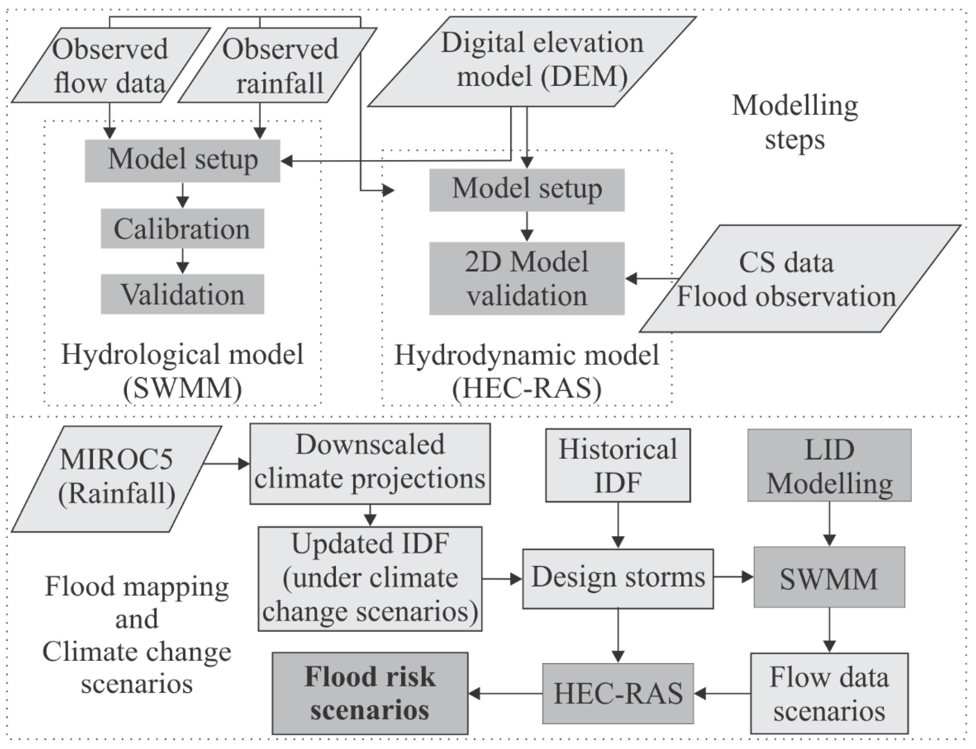
Rainfall data was registered at 10 min intervals between September 2013 and November 2020. The input data come from a rain gauge installed inside the Gregório Creek catchment. The gauge location was close to the flooding area and approximately in the boundary of the area where hydrodynamic simulation was performed (2D area, Figure 1).

3. Methodology

In this study, the SWMM model was selected as a computational engine to simulate the resulting flow from several design storms at the actual scenario of Gregório Creek catchment and for future conditions considering climate changes. After this, HEC-RAS was chosen to perform a 2D rain-on-grid simulation using SWMM inputs as a boundary condition and citizen science data (CS data) for model validation. After model validation, we used it to achieve the flood scenarios for the current and future situation of the catchment due to climate changes—Figure 2 details the main steps performed towards generating flood risk scenarios. The purpose is to assess the dynamic resilience of the system and flood risk by obtaining flooded area scenarios, representing the risk component related to the hazard and exposure.

3.1. Hydrological and Hydraulic Modelling

The USEPA Storm Water Management Model (SWMM) is a computational program capable of simulating the rainfall runoff transformation over a catchment [40]. The model has a hydrological and a hydraulic modelling module capable of simulating single events or long-term simulations of runoff quantity and quality in micro- and macro-drainage of urban catchments. The runoff component of SWMM is lumped and conceptual at the subcatchment scale and is responsible for receiving rainfall and generating runoff and pollutant loads. The routing module transports the surface runoff from the hydrological model along rivers, canals, and other conduits [68]. SWMM is a semi-distributed model, as the user can define the number of subcatchments according to the level of discretization desired [69].

Gregório Creek catchment was modelled using SWMM, setting the dynamic wave equations and the SCS curve number (CN) method for the model routing and infiltration module. The inputs used for model set-up were width, average slope, infiltration, Manning’s coefficient for the pervious and impervious area (N-perv and N-imperv, respectively), percentage of impervious area with no depression storage, depth of depression storage on pervious and impervious areas, the percentage of impervious area (%Imperv), and canal roughness. Aiming to keep the physical meaning of the model, two groups of model features with a different range of parameters value were defined, one for highly urbanized areas and other for green areas. The curve number and percent of impervious area parameter groups were defined based on the map of land use of São Carlos city [70].

As a multi-parameter model, many methodologies to calibrate SWMM have been developed [60,71]. We performed model calibration using an automatic calibrator that uses genetic algorithms for optimization developed by [72]. The stop criteria is based on the deviation between the evaluation function of the best set of decision variables found for the current generation $\left(n\right)\left[f\left(x_n\right)\right]$ and the one of the previous generation $\left[f\left(x_{n-1}\right)\right]$. A threshold of 0.0001 was defined; when the deviation is lower than that value during three generations in sequence, the optimization process stops.

Table 1. Calibration settings.

Genetic Algorithm	Settings
Two-point crossover probability	0.8
Flip bit mutation probability	0.05
Individuals’ selection	Tournament selection
Decision variables (parameters)	CN, %Imperv, Roughness, N-perv, N-imperv
Population size	50
Generations	100
Objective function (OF)	NSE
Stop criteria	$\left|f\left(x_n\right)-\right|f\left(x_{n-1}\right)/f\left(x_n\right)\le 0.0001$

shows the calibration settings.

Seven rainfall events between September 2013 and January 2014 were divided into two groups according to the average intensity of the rainfall: moderate and heavy—according to the American Meteorological Society [73] classification. Then, the events were chosen at random for two groups: calibration and validation (

Table 2. Rainfall events and the resulting water depth peak used for calibration and validation of the hydrological and hydrodynamic models.

Hydrological Model (SWMM)
Event	Date (Day Month Year)	Rainfall intensity (mm/h)	Total rainfall (mm)	Peak water depth (m)
Calibration
Event 1	3 September 2013	6.13	63.2	1.20
Event 2	25 March 2013	16.07	46.6	1.35
Event 3	28 May 2013	4.58	75.8	1.14
Event 4	29 November 2013	13.8	35.2	1.26
Validation
Event 1	4 October 2013	4.41	58.4	1.23
Event 2	20 December 2013	14.63	17.8	0.52
Event 3	14 January 2014	3.19	42.6	0.95
Hydrodynamic model (HEC-RAS)
Validation
Event 1	23 November 2015	2.21	16.6	0.85 *
Event 2	20 March 2018	37.42	68.6	0.75 *
Event 3	12 January 2020	21.47	94.2	0.72 *
Event 4	13 November 2020	8.07	39	0.28 *
Event 5	26 November 2020	8.77	38	1.65 *

* Citizen science data collected during the flood events may not represent the maximum water depth that occurred.

). The Nash–Sutcliffe efficiency (NSE) was used as OF and to assesses model accuracy. Model calibration resulted in an NSE value of 0.63 for the calibration period and 0.51 for the validation period. Table 2 presents the events selected.

The rainfall runoff transformation was made on SWMM to feed the hydrodynamic model (HEC-RAS) with different flow values to compare water depth reached when considering LIDs insertion and climate changes. The flow data used for the model’s accuracy evaluation came from a sensor installed near the catchment outlet (Figure 1); then, the entire catchment was modeled and calibrated on SWMM based on the inference made at this location. Though the whole catchment was modeled, the flow outputs that fed the HEC-RAS model were accessed in an intermediary location of the catchment near the 2D area border and at the Gregório Creek.

3.2. LID Modelling

SWMM can explicitly model eight types of LID controls: rain gardens, bioretention cells, infiltration trenches, porous pavements, rain barrels, vegetative swales, rooftop disconnection, and green roofs. The bioretention cells modelled in SWMM are depressions containing vegetation grown in soil mixture placed above a gravel drainage bed, which provides storage and infiltration of the runoff captured from surrounding areas [50] as a vertical layer. The flux and storage of water resulting from each layer are tracked at each model time-step. The LID practice’s flow is combined with the subcatchments’ runoff to establish the aggregate values for each process at the end of every time step [74]. We choose the bioretention cells as LID control to simulate its impacts on water depth peaks and flood spots at the Gregório Creek.

The input data used for the bioretention cells were calibrated by a previous study developed by [75] for the city of São Carlos in an adjacent catchment of Gregório Creek. The study built a prototype and performed field experiments with observed rainfall events to determine all the coefficients. Each cell had an area of 12 m².

In the SWMM model, the rainfall runoff component was lumped and conceptual at the sub-basin scale. The Gregório creek catchment was discretized into 13 sub-basins, with areas ranging from 0.67 km² up to 4.71 km², according to their main natural sources. The sub-catchments had their area divided into pervious and impervious portions. The LIDs were designed to capture the runoff coming 100% from the catchment’s impervious areas. From this, we modeled the LIDs on the sub-catchments until they corresponded to 1% of each sub-area. The outflow from the LIDs was sent to the catchment’s pervious portion.

Table 3. Input data * for the bioretention cells modelled on SWMM.

Surface	Value Adopted	Typical Range **	Soil	Value Adopted	Typical Range **
Storage depth (mm)	600	-	Thickness (mm)	1000	450–900
Vegetative volume fraction	0.1	0.1–0.2	Porosity	0.32	0.45–0.60
Storage			Field Capacity	0.43	0.15–0.25
Thickness (mm)	500	100–150	Wilting Point	0.12	0.05–0.15
Void ratio	0.4	0.12–0.21	Conductivity (mm/h)	195.48	50.80–1397
Seepage rate (mm/h)	5.83	-	Conductivity slope	46.38	30–60
Clogging factor	0	-	Suction Head	66.98	50.80–101.60

* Values calibrated by [55]; ** Typical range from [40].

presents the main parameters used for the bioretention cells set-up.

To evaluate the performance of the LID practices, runoff retention efficiency and peak flow attenuation efficiency were calculated according to Equations (2) and (3).

$$Ef{f}_{rr}=\frac{V_{in}-V_{over}}{V_{in}}$$

(2)

$$Ef{f}_{peak}=\frac{Q_{peak,in}-Q_{peak,over}}{Q_{peak,in}}$$

(3)

where: $Ef{f}_{rr}$ is the runoff retention efficiency; $V_{in}$ (m³) is the total inflow volume; $V_{over}$ (m³) is the total overflow volume; $Ef{f}_{peak}$ is the peak attenuation efficiency; $Q_{peak,in}$ (m³/s) is the maximum inflow value; $Q_{peak,over}$ (m³/s) is the maximum overflow value.

3.3. Hydrodynamic Modelling

The Hydrologic Engineering Center’s (HEC) River Analysis System (HEC-RAS) software is capable of performing steady flow simulations and one-dimensional (1D) and two-dimensional (2D) unsteady flow analysis. The HEC-RAS system comprises a graphical user interface, separate hydraulic analysis, and mapping facilities (HEC-RAS Mapper) [76]. HEC-RAS can perform coupled 1D and 2D modelling and 2D modelling with no 1D elements. We used the second option to reproduce the hydrodynamic modelling of the Gregório flooding area.

To perform the 2D HEC-RAS rain-on-grid simulations, the Advanced Land Observing Satellite Digital Elevation Model (ALOS DEM) with a spatial resolution of 12.5 m was used to represent surface terrain. We used this input due to a lack of more accurate terrain information for the area. Several hydrological studies have already been carried out in the region [77,78,79,80]. Still, none of them performed measurements or purchased more accurate images, which is a reality in many river basins in developing countries.

The HEC-RAS model geometry was set up in the HEC-RAS mapper. The 2D area (Figure 1, map on the top right) is defined as the boundary for which 2D computations occur, a computational mesh based on the DEM is created within the 2D flow area. The delineation of the 2D area was made as a sub-catchment delineation, where the inlet point was defined as the location at Gregório Creek immediately upstream of the main flooding area (the Municipal Market region).

An unsteady flow plan (2D only) including rain-on-grid rainfall time-series and a flow input as upstream boundary condition was created in HEC-RAS. This flow input came from the SWMM simulations at the location in Grregório Creek near the 2D area boundary. The unsteady flow routing was performed using diffuse wave momentum equations. Rainfall inputs were at a 10 min time-step distributed uniformly throughout the catchment area and flow data at a 5 min time-step. The value adopted for the global roughness was 0.01 [81]. Computational interval is an end-user-defined parameter that defines the temporal resolution of hydrodynamic calculations [82]. The hydrograph output interval was set to every 5 min and the mapping output interval each hour. A 15 s computational interval was determined to achieve satisfactory accuracy at HEC-RAS output, considering the rapid response from urban floods and the spatial scale and resolution of the project.

There are no flood monitoring data from sensors for the Gregório catchment. Buarque et al. [56] developed a socio-hydrological study and validated an urban flood model as one of its methodological steps. In order to validate the model, they extracted records of water depths in the streets from pictures provided by witnesses of the flood events. Furthermore, they collected the water depth in loco after the events using the mark left on the walls. They used the CAFLOOD application to develop the flood model, a low-complexity model capable of providing fast and accurate urban flood simulations based on a cellular automata approach [83]. The model uses the DEM, rainfall intensity, and global roughness as primary inputs.

The main purpose of their study in the Gregório Creek was to replicate the socio-hydrological mechanisms and design possible scenarios resulting from the interaction between water and human variables instead of seeking to best capture the catchment hydrodynamic behavior [56]. Even though the model reached satisfactory results (RMSE = 0.62), the same model approach could not be applied for our study as the CAFLOOD model is unsuitable for using flow time series as input data. To capture flow changes at the catchment due to LID controls set-up and its influence on flood spots, we needed to couple the hydrological simulations on SWMM with the 2D unsteady flow analysis at HEC-RAS.

We followed a similar approach to validate the 2D HEC-RAS for Gregório Creek and used a dataset provided by [56] (Events 1–5, Table 2). Model calibration was not performed due to the lack of data. The five flood events obtained from the cited study were used for the 2D model validation (Figure 1, Event 1–5). The model performance was inferred at the pixel closest to the water depth observation location (RMSE = 0.52). Figure 3 demonstrates the model outputs used for accuracy assessment during the validation events.

3.4. Design Storms

Design storms were used as input for scenarios simulation of current and future perio5ds with climate change. For the construction of the storms, the alternating block method [84,85,86] with different configurations of duration, return period, and temporal distribution was adopted to obtain ranges of variability. Variability assessment was proposed by [87] as an alternative to uncertainty assessment for climate change scenarios due to the difficulty of accessing statistical uncertainty of GCM and RCM itself, in addition to downscaling and bias correction methods.

As for duration, three different intervals were adopted: 30 min, 1 h, and 2 h, representing more intense and more recurrent rainfalls in the city of São Carlos. As for the return period (RP), 5, 10, 50, and 100 years were adopted to obtain a variability between higher recurrence and lower intensity and lower recurrence and extreme intensity. Finally, two patterns of temporal distribution were adopted: centralized (Ce) and delayed (At) (similar to Huff’s third quartile [88,89]). The delayed pattern was included to represent scenarios with higher runoff generation. In this temporal pattern, the initial and less intense rainfall is responsible for saturating the soil. At peak intensity, the infiltration of water is lower, leading to more significant runoff and higher flow peaks.

For the current period, the design storms were constructed using the standard intensity–duration–frequency curve (IDF) for the city of São Carlos [90] (Appendix A). Regarding future periods, the updated IDFs with climate change developed by [75] were adopted for the periods from 2015 to 2050 and 2050 to 2100 (Appendix A). The future IDFs were updated using the daily rainfall data obtained by the RCM Eta-MIROC5 [16,17] for the scenarios, RCP 4.5 and 8.5 (representing optimistic and pessimistic variabilities) bias-corrected by the methods power transformation (PT), and distribution mapping (MD).

The combination of all design storm configurations and evaluation scenarios resulted in 216 input rainfalls for hydrological and hydrodynamic simulation. Storms were selected to better visualize the results, representing weak, moderate, strong, and extreme intensities for the current and future periods defined according to extremes of the return periods and rainfall duration, presented in

Table 4. Representative design storms.

	Duration (min)	RP (years)	Temporal Distribution *	Period	RCM	Bias Correction **	RCP
Weak	30	10	Ce and At	Current	-	-	-
Moderate	60	10	Ce and At	Current	-	-	-
Strong	60	50	Ce and At	Current	-	-	-
Weak	30	10	Ce and At	2050	MIROC5	PT and MD	4.5 and 8.5
Moderate	60	10	Ce and At	2050	MIROC5	PT and MD	4.5 and 8.5
Strong	60	50	Ce and At	2050	MIROC5	PT and MD	4.5 and 8.5
Extreme	120	50	At	2100	MIROC5	PT and MD	4.5 and 8.5

* Rainfall hydrograph centralized (Ce) and delayed (At); ** bias-correction by power transformation (PT) and distribution mapping (MD) methods.

.

3.5. Dynamic Resilience

To assess resilience, the STDRM approach [30] was used, here called dynamic resilience. In this approach, resilience was presented as a unitary variable representing the system’s performance losses during a disruptive event and its subsequent recovery.

As a first step to evaluate dynamic resilience, it is necessary to establish the system performance evaluation metrics. In this study, the peak water depth at the most critical point of the catchment along with the event—$h_c\left(t\right)$—was considered a performance indicator. The most critical point (Figure 1) was defined from physical and social characteristics, i.e., water depth and associated economic losses.

Finally, the resilience—$r\left(t\right)$—was calculated according to Equation (4) as a function of the normalized performance, i.e., dividing it by the system’s maximum performance considering all the events evaluated—$h_{c,max}$ (m). Resilience was deemed to be maximum if the floodwater depth was lower than the minimum water depth for houses and stores flooding—$h_{c,min}$ (m).

$$r\left(t\right)=\{\begin{array}{c}if{h}_c\left(t\right)\le h_{c,min},1\hfill \\ if{h}_c\left(t\right)>h_{c,min},1-\frac{h_c\left(t\right)}{h_{c,max}}\hfill \end{array}$$

(4)

4. Results

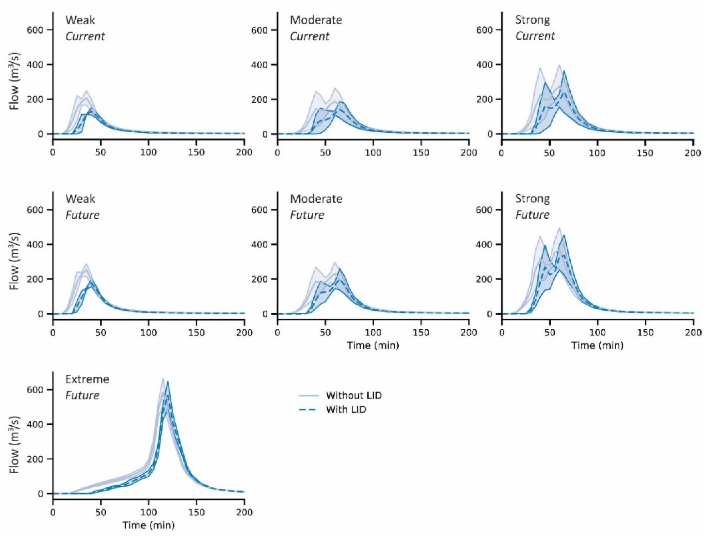
4.1. Hydrological Scenarios

After the SWMM calibration and validation, different climate scenarios and structural intervention for risk management were simulated for the current and future periods, considering climate change. Figure 4 shows the simulated hydrographs at the midpoint of the Gregório basin (2D model input) with the input of representative design storms considered weak, moderate, strong, and extreme for the different scenarios, presented in Table 4.

It is possible to notice from Figure 4 that peak flows for current periods varied between maximum values of 246.7 m³/s to 398.6 m³/s considering no risk management intervention. In intervention scenarios (Table 4) with LID practices, these values were reduced between 78 m³/s and 97 m³/s, representing an attenuation of approximately 40% and 30% for weak and moderate design storms, respectively. However, for heavy storms and maximum peaks in the most extreme scenario, the peak flows were reduced by only 35 m³/s, representing a 9% reduction.

In the future scenarios presented in Figure 4, there was an increase in the maximum peak values between 72 m³/s and 235 m³/s when compared with the current period, considering scenarios of weak, moderate, and heavy design storms and without the intervention of LID practices. The application of bioretention cells collaborated to reduce the peak increase to a range of 78 m³/s to 221 m³/s for scenarios with LID intervention.

The intensification of rainfalls in future periods due to climate changes reflects on the efficiency of bioretention to mitigate peak flows. This drop was more accentuated for the moderate rainfall scenario (from 78 m³/s to 35 m³/s, equivalent to an efficiency drop from 30% to 10%). For heavy storms, the peaks were reduced by 35 m³/s in the current period and 50 m³/s in the future period, equivalent to an efficiency drop of 9% to 8%. Even with higher peak flow reductions for future periods, there was a reduction in the system’s overall efficiency. In the case of an extreme storm for the final year of 2100, the flow reductions were even less significant when evaluating the implementation of LID practices. There was a reduction in maximum peak by 31 m³/s, representing a 4% efficiency of peak attenuation. From the hydrographs, it is also possible to observe that bioretention cells contributed to a delay in the occurrence of peak flow between 5 and 10 min.

In addition to the hydrographs evaluation for the representative storms, the reduction in volumes and peak flow for all scenario combinations and the current and future periods were also evaluated (Figure 5). There was a general increase in runoff volumes and peak flows for future periods with climate change. The increase was significant and more pronounced for higher RPs (50 and 100 years) than smaller RPs.

Considering the scenarios without LID practices, there was an increase of 25.7 m³ and 56.9 m³ in the medians for RP 5 years (representing a relative increase of 1.2× and 1.4) for periods 2050 and 2100, respectively. For 100 year RP in the same periods, there was an increase of 98.6 m³ and 111.3 m³, representing a relative increase of 1.8× and 1.9×, respectively.

Furthermore, there is an increase in the variability of volumes for the larger RPs, both for the current period and for future periods (Figure 5). In future periods, the variability was more accentuated with a greater tendency to higher values [87]. As for peak flows, the variability was more constant among all RPs but increased when comparing the future periods with current periods.

From Figure 5, it is also noted that the LID practices could reduce the runoff volumes in values within a fixed range of approximately 45 m³ to 55 m³. This interval represents the volume retention capacity of all bioretention cells applied together in the catchment. The variations are relative to the soil saturation level and therefore its infiltration capacity. Similar results were observed in [75]. This reflects on the peak flow attenuation, which also presented limitations. In Figure 4, it is possible to observe that the maximum peaks were reduced to values approximately around 30 m³/s. Therefore, the drop inefficiencies over time (Figure 6) are related to an increase in rainfall volumes and peaks while keeping the maximum capacity of bioretention constant.

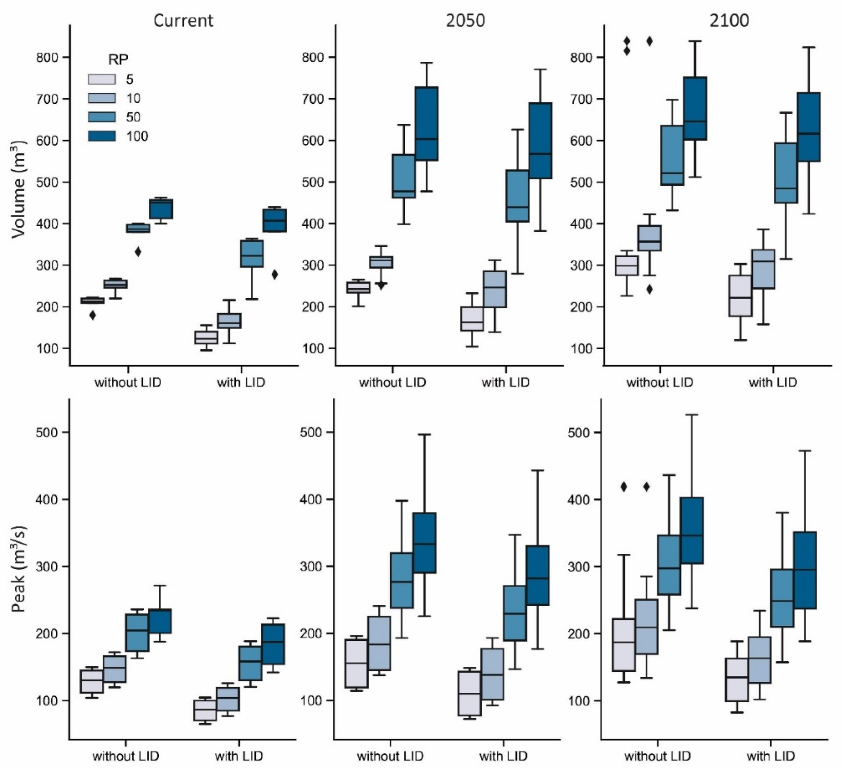
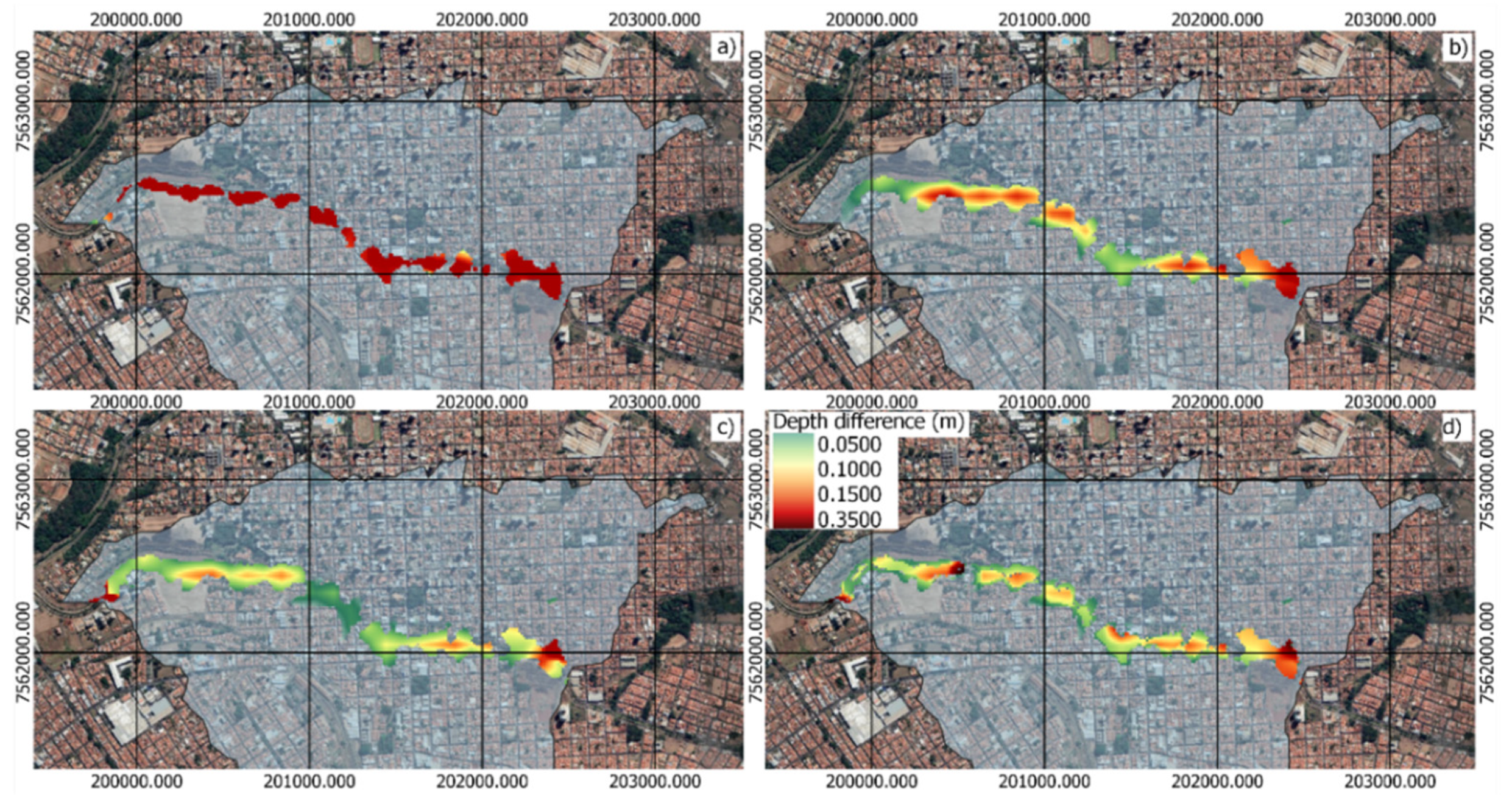
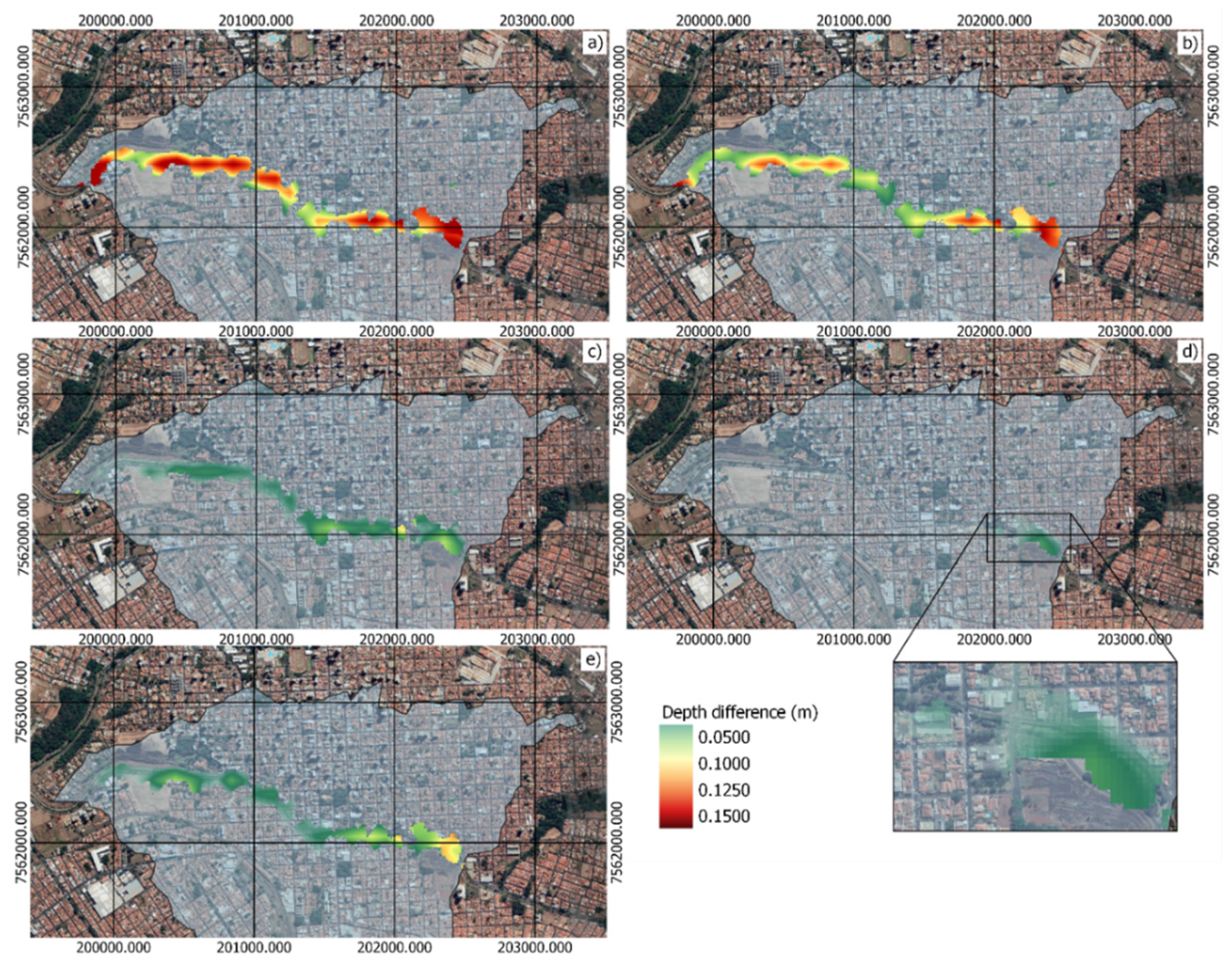
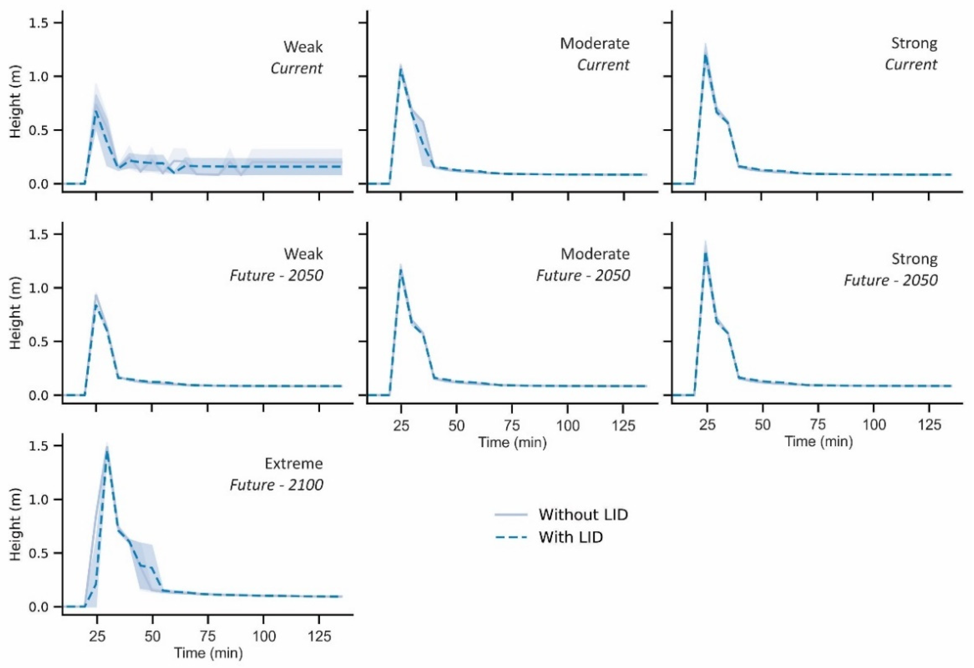
4.2. Hydrodynamic Scenarios

The HEC-RAS model was validated for 2D rain-on-grid simulations. The flow hydrographs simulated using SWMM for all the climate scenarios, with and without LID interventions, and the rainfall for the different climate scenarios (Table 4) were used as inputs to HEC-RAS to assess its effects over the flooding area. Figure 7 shows these results by comparing the changes in peak water depth in the flooding area for weak, moderate, and strong scenarios of rainfall for the current situation of the catchment when adding LID interventions and without LID intervention.

The results obtained in the spatial distribution of events reinforced the results of Section 4.2 (simulated scenarios using SWMM). The reduction in the flood spot peaks was strongly noticed for weak rain with a predominance of about 30 cm reduction in the maximum depths for this scenario (Figure 7a) whereas for a heavy rain scenario, the decline of the peak between 5 and 10 cm was more noticeable (Figure 7c). LID interventions mitigated the risk of flooding but were more notable for less extreme events.

Figure 7d presents the difference between the average peak water depths for all scenarios with and without adding LID practices to evaluate the average performance of flooding area peaks reduction by introducing bioretention cells over the catchment, when considering the current climate scenario. The maximum average difference in peak water depth was about 0.35 m.

Figure 8 shows the efficiency of bioretention to mitigate peak flows in future periods due to climate changes. Compared to the current climate condition, the LIDs efficiency decreasing for climate change scenarios was remarkable, especially for strong and extreme rainfall events (Figure 8c,d). Even when focusing on weak rainfall, water peak reduction due to adding bioretention cells dropped from a maximum decrease of 0.35 m for the current scenario to 0.15 m for future climate conditions.

A slight reduction in peak water depth over the flooding area could be noticed for heavy storms, with a maximum reduction of about 0.1 m (Figure 8c). In the case of an extreme storm for the year 2100, the peak water depth reductions over the flooded spot were even less significant when evaluating the implementation of bioretention cells (Figure 8d); the only effect on water depth peak reduction seen was about 0.05 m at the most upstream area of the 2D mesh.

Figure 8e shows the difference between the average peak water depths for all scenarios with and without adding LID practices to evaluate the average performance of flooding area peaks reduction by introducing bioretention cells over the catchment when considering climate changes. The maximum average difference in peak water depth was about 0.15 m. When comparing the average drop of water depth peaks for the climate change scenario (a maximum average reduction of about 0.13 m, Figure 8e) with the current climate scenario (a maximum average drops of about 0.35 m, Figure 7d), the efficiency decreasing of the LID cell’s introduction due to climate changes became evident.

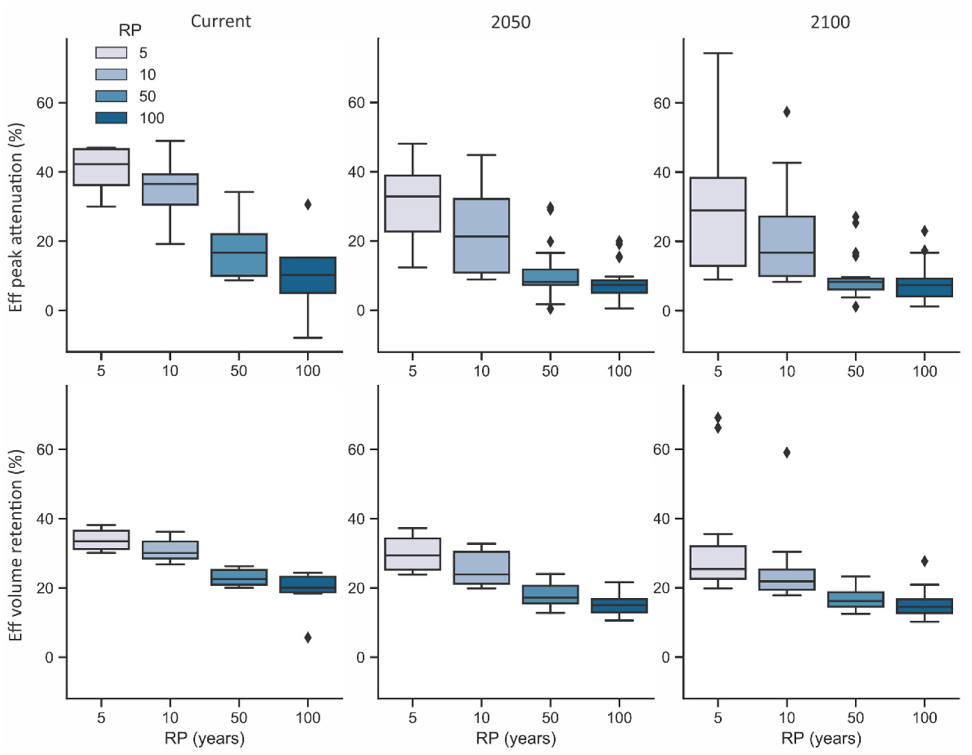
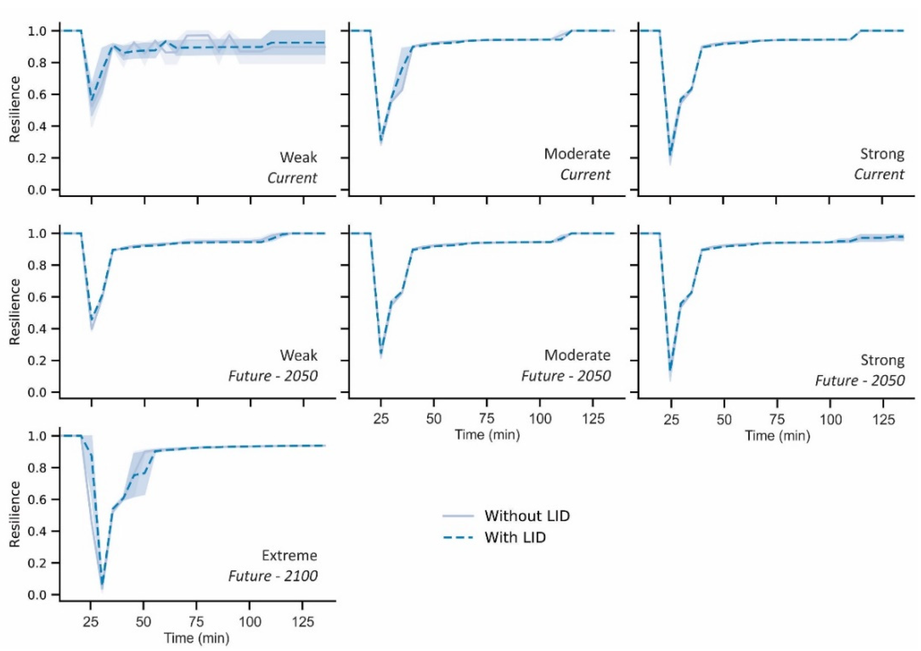
4.3. Dynamic Resilience

For the evaluation of dynamic resilience, the system’s performance was first obtained from the assessment of water depths over time at the critical point of the catchment (Figure 1—resilience inference) for the representative storm scenarios and intervention measures (Appendix B). The performances were normalized according to Equation (4) to obtain the unitary resilience during the event (Figure 9).

The scenarios with the greatest resilience were those of weak storms in which the resilience reached its worst values around 0.6 and 0.4 for both the current and future periods. Regarding the minimum extreme of the variation range, without LIDs, the resilience values reached minimums of 0.39 and 0.37 for the current and future periods, respectively. With LID practices, the resilience reached minimum values around 0.45 and 0.6. For the moderate to extreme scenarios, the increase in resilience with LIDs was slight, around 0.01, which was not significant.

From Figure 9, it is possible to observe that there was a more significant time until the resilience began to drop in scenarios with LID practices. In the case of an extreme storm, the resilience reached minimum values of 0 and 0.023 with and without LID, respectively. However, it reached worse values faster (greater slope of the recession curve), i.e., bioretention cells contributed to a more abrupt reduction in resilience. In addition, a longer delay for full recovery was also observed (smaller slope in the recovery curve). The combination of two factors could explain this behavior: (1) the considered scenarios presented rainfall of 120 min, and (2) the LID practices were able to delay the peak flow occurrence by up to 10 min. Therefore, the maximum values and their recession occurred after the peak of hydrographs without LID.

5. Discussion

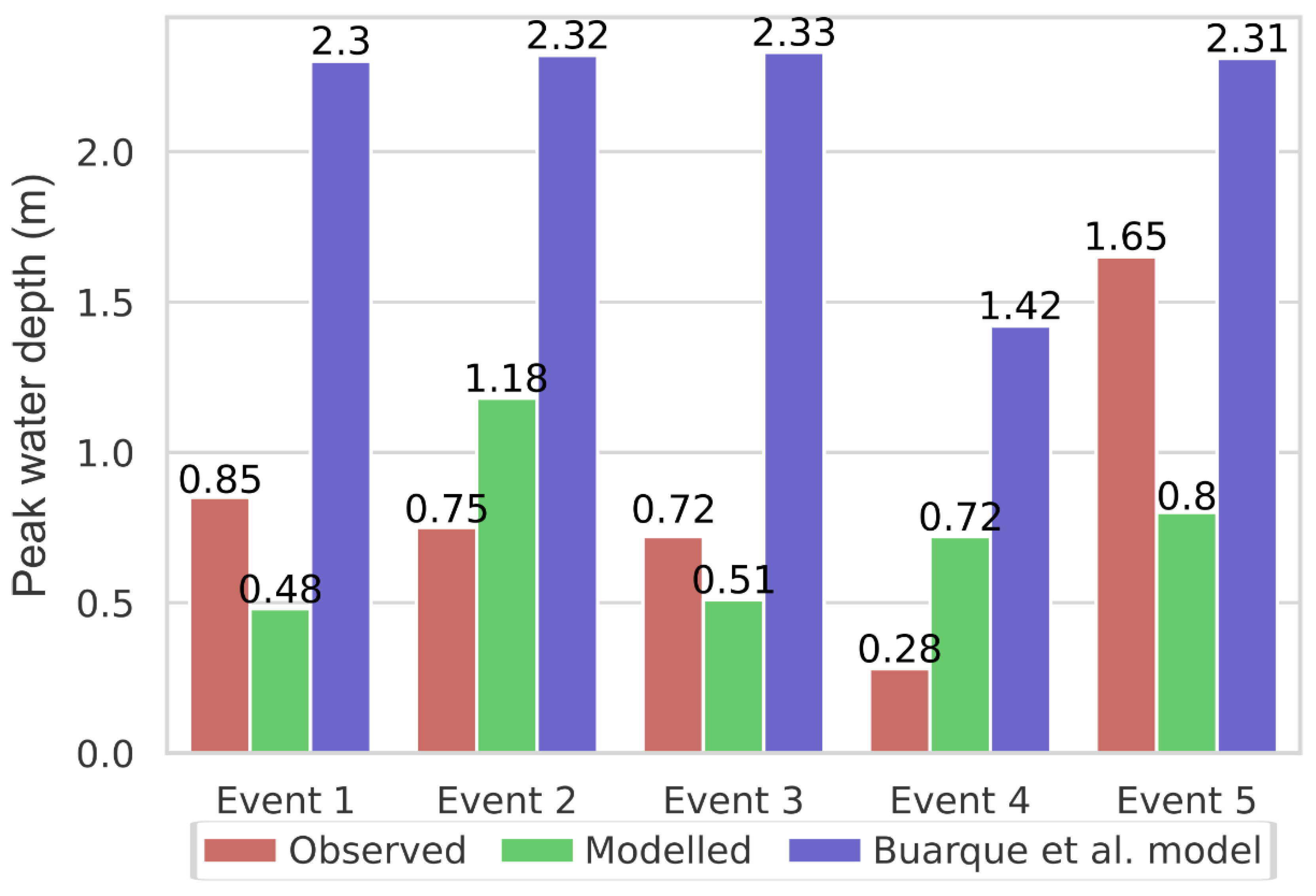
5.1. Coupled 1D and 2D Model Accuracy

Studies [91,92] discussed that optimal values for flood extent and flood depth are obtained for hydrodynamic models not calibrated when using DEM or Digital Terrain Models (DTM) with resolution of 2 m. This data resolution can be obtained by airborne light detection (LiDAR), aerial photography, and topographical maps. However, these types of data are frequently not available in poorly gauged and ungauged basin or are not open source and presents high associated costs, especially in developing countries. Using terrain data with less resolution that can lead to less accuracy in the hydrodynamic models is a common reality in those locations.

Examples of studies with coupled hydrological and hydrodynamic modelling approach performed with DEM data with 10 m resolution for poorly gauged basins could be found in [37] for Toronto, Canada, [39,93] in India, and [45] in Missouri, USA. In those studies, the basins evaluated ranged from 6.8 km² to 658.9 km². Therefore, application purposes of flood maps obtained by hydrodynamic models with less accuracy must be discussed.

Additionally, the majority of these studies have not performed a calibration and validation for the hydrodynamic modelling. An exception is the study of Jha and Afreen (2020) that calibrated both SWAT and HEC-RAS models independently; however, the calibration of HEC-RAS was made for peak flows and not for flood extent and flood depth. In the same sense, [92] also performed a calibration and validation for HEC-RAS considering discharges and peak flow. In their study, they discussed that calibrating the hydrodynamic model was difficult due to the uncertainties in the parameters and variables, especially rainfall depth and discharge data synchronization.

Ref. [49] also discussed that calibrating flood extension and flood depth was a difficult process because it requires spatial data. Spatial data can be obtained from remote sensing, but during rainfall events it is difficult to obtain cloud-free images, impairing the water depth classification. Additionally, the images may also lack synchronization with the flood event.

To overcome this problem, in this study, we proposed an alternative methodology to acquire spatial data using citizen science that can be used for model calibration and validation. Here, we opted for the Manning coefficient from the literature (n = 0.01) [81] to validate the model due to few monitored events. From Figure 3 and the obtained NSE = 0.52, the model accuracy was considered average and could be improved by calibration of Manning coefficient and infiltration process after obtaining more citizen science data for other flood events.

In general terms, the hydrodynamic model tended to overestimate the flood depths (Figure 3). Other studies [39,93] with coupled hydrological models with HEC-RAS and without calibration have adopted roughness values of 0.025 and 0.03. The higher value of global roughness adopted in this study may be one of the reasons to obtain higher flood depths. Additionally, the coarse resolution of DEM used generated higher uncertainties in the model.

Finally, as mentioned before, the purpose of applying hydrodynamic models to obtain flood maps must be discussed, particularly in partially gauged or ungauged basins. Study [37] stated that the major purpose of evaluating the flood maps for different future scenarios (climate, land use, or mitigation intervention) is to evaluate the difference between them rather than to obtain flood precision. A similar discussion was made by [56] in their study for the Gregório Creek where they highlighted that the best capture of the catchment hydrology was not their main purpose.

Therefore, it is important to highlight that this approach of coupled hydrological and hydrodynamic model, calibrated or validated with citizen science data, has the main purpose to serve as a tool to contribute to a risk-informed and evidence-based decision-making process in poorly gauged or ungauged catchments. For example, the results obtained in this study supports the decision that LID practices can be used as mitigation measures to more recurrent events (RP less than 10 years) and it is necessary to guarantee more than 1% cover with LID practices to mitigate the non-stationary effects of future climate projections.

5.2. Urban Flood Mitigation Scenarios

For weak and moderate design storms in the current scenario, the intervention scenario with LID practices was able to mitigate peak flows by approximately 40% and 30%, respectively. These results are similar to those obtained by [49] for rainwater harvesting applied, decentralized, and distributed in the basin using the same SWMM and HEC-RAS coupled methodology. Additionally, in agreement with these results, several studies showed that LID practices, especially bioretention, are more efficient and (therefore) recommended for more recurrent and less intense rainfalls [94,95,96].

However, when considering the effects of climate change in the design rainfalls, there was a drop in peak flow attenuations. For the moderate rainfall scenario, the peak mitigation was reduced to only 10%. The drop in efficiencies over time (Figure 6) was related to an increase in rainfall volumes and peaks while keeping the maximum capacity of bioretention constant. Therefore, there is a need to increase the practice’s useful volumes. This can be done by:

(1)

Increasing the bioretention volume of each practice over time. In this sense, [28,75] discussed the importance of incorporating future climate change scenarios in the conception and design of bioretention structures based on a modular design that allows the expansion of their areas and volumes over pre-defined periods.

(2)

Increasing the total bioretention volume in the entire catchment, i.e., increasing the number of practices applied in the catchment.

It should be noted that this study evaluated a scenario with the implementation of bioretention cells corresponding to 1% of the catchment area (due to the availability of space-related to the current occupation of the soil in the city of São Carlos).

LID practice manuals recommend coverage of 1% to 5% of the total area of the catchment as optimal values for flood control [97,98,99]. Additionally, [100] recommended rates of 10% to 20% between the bioretention area and the impermeable area to obtain optimal exfiltration and groundwater recharge. However, these metrics do not consider the changes in climate patterns in future scenarios and may lead to areas that are smaller than necessary for good performances, as observed in the results from this study.

One of the complementary purposes of this study was to assess whether LID practices can at least mitigate the surplus generated by climate change on river discharges and consequently flood depths, keeping the volumes and peak flows constant and equal to the values of the current period. From Figure 5, it is possible to notice that the proposed level of coverage by bioretention was not sufficient to guarantee this mitigation. However, as shown in Figure 6, the efficiency of these techniques with only 1% coverage of the total catchment area (a viable scenario in terms of spatial availability) could maintain average efficiencies of around 35% for more recurring rainfall depths.

Finally, for resilience evaluation, it was possible to observe a more significant variability in the resilience curve for the weak storms and the current period. This is because the LID practices have higher volume retention and peak attenuation efficiencies for weak storms. The effects varied depending on the rainfall pattern, presenting different final reductions in the peak water level. The efficiencies were reduced for moderate and heavy storms, with no significant decreases in the flooded water level (as discussed in Figure 5) and resilience, regardless of the scenario.

6. Conclusions

This research proposed a novel approach of coupling the hydrological model SWMM and the hydrodynamic model HEC-RAS calibrated and validated with citizen science data for modelling a partially gauged urban basin. This approach was applied to simulate the effects of adding bioretention cells on the system’s resilience for several rainfall scenarios that considered different return periods and climate changes. The methodology was applied at the Gregório Creek catchment. The effects on the system’s resilience by adding LID practices were evaluated by comparing the model’s outputs for all the rainfall scenarios with and without the bioretention cells modelled on SWMM.

The results showed that LID practices can reduce peak flows by around 30% to 40% for moderate and weak rainfall, respectively, in the current climate scenario. However, when considering the effects of climate change, the efficiency for moderate rainfall dropped to only 10%. As for heavy rainfall, in the current climate scenario, the peak retention efficiency was significantly smaller than compared with moderate and weak rainfalls, with values around only 9%. In the future scenario, this efficiency dropped to 8%, representing a less accentuated drop than for less intense rainfall. This happens because bioretention has a maximum storage capacity, which is responsible for its mitigation effect. This maximum capacity was already reached in the current extreme rainfall scenarios; thus, there were no significant reductions in future scenarios with climate change.

These effects on main channel flows were reflected in the flood map generated by the hydrodynamic model and consequently in the resilience assessment. For more extreme rainfall and future climate change scenarios, the reductions in flood depth and increases in resilience were minimal. This demonstrates that the total volume retention capacity of LID practices was undersized, requiring an increase in their individual volumes (modular expansion) or an increase in their coverage in the basin (>1%).

The hydrological simulation coupled with hydrodynamics allowed establishment of maximum peak water depths that represent acceptable risks and desired resilience. From these goals, the optimal intervention scenario could be selected (e.g., minimum coverage of LID practices over time). The modular design of LID practices or the expansion of their coverture in the catchment over time can be a viable alternative for long-term planning, both in terms of risk management actions and economic resource availability. Planning to increase the coverage of LID practices through policies to encourage their individual and decentralized adoption as well as their implementation through the local government can contribute to at least keep the current flood risk constant for future climate change scenarios (which was not achieved with the intervention scenario proposed in this study).

We strongly suggest performing uncertainty analysis for future studies, as data coming from citizen observatories are subject to significant uncertainty beyond the complexities in both models used (SWMM and HEC-RAS). Moreover, the methodology was only tested as a case study on the Gregório Creek catchment applying bioretention cells. Further comparison using different green infrastructure measures such as porous pavements, rain barrels, vegetative swales, and green roofs as well as in other catchments may foster sustainable approaches towards systems resilience improvement and mitigation of climate changes effects. Furthermore, adopting criteria of selecting check-points decentralized across the watershed to assess runoff retention efficiency and peak flow attenuation efficiency spatially distributed may provide a better understanding of measures to take and find the optimal distribution of LID practices over the area.

References

1. Hederra, R. Environmental sanitation and water supply during floods in Ecuador (1982–1983). Disasters 1987, 11, 297–309. [Google Scholar] [CrossRef]
2. Ahmed, M.F.; Ashfaque, K.N. Sanitation and Solid Waste Management in Dhaka City During the 1998 Flood. In Engineering Concerns of Flood, 1st ed.; Ali, M.A., Seraj, S.M., Ahmad, S., Eds.; Directorate of Advisory, Extension and Research Services Bangladesh University of Engineering and Technology: Dhaka, Bangladesh, 2002; Volume 1, pp. 1–13. ISBN 984-823-002-5. [Google Scholar]
3. Baig, S.A.; Xu, X.; Navedullah, M.N.; Khan, Z.U. Pakistan’s drinking water and environmental sanitation status in post 2010 flood scenario: Humanitarian response and community needs. J. Appl. Sci. Environ. Sanit. 2012, 7, 49–54. [Google Scholar]
4. Bastawesy, M.E.; Ella, E.M.A.E. Quantitative estimates of flash flood discharge into wastewater disposal sites in Wadi Al Saaf, the Eastern Desert of Egypt. J. Afr. Earth Sci. 2017, 136, 312–318. [Google Scholar] [CrossRef]
5. Leopold, L.B. Hydrology for Urban Land Planning: A Guidebook on the Hydrological Effects of Urban Land Use; USA Geological Survey: Washington, DC, USA, 1968; Volume 554. [Google Scholar]
6. Wong, T.H.F.; Eadie, M.L. Water Sensitive Urban Design—A Paradigm Shift in Urban Design. In Proceedings of the 10th World Water Congress, Copenhagen, Denmark, 16 December 2000; Available online: http://gabeira.locaweb.com.br/cidadesustentavel/biblioteca/%7B30788FE6-98A8-44E5-861E-996D286A78B3%7D_Wong1.pdf (accessed on 1 April 2018).
7. Konrad, C.P.; Booth, D.B. Hydrologic changes in urban streams and their Ecological significance. Am. Fish. Soc. Symp. 2005, 47, 157–177. [Google Scholar]
8. Stark, B.; Ossa, A. Ancient Settlement, Urban Gardening, and Environment in the Gulf Lowlands of Mexico. Lat. Am. Antiq. 2007, 18, 385–406. [Google Scholar] [CrossRef]
9. Nunes, M.F.; Figueiredo, J.A.S.; Rocha, A.L.C.D. Sinos River Hydrographic Basin: Urban occupation, industrialization and environmental memory. Braz. J. Biol. 2015, 75, 3–9. [Google Scholar] [CrossRef] [Green Version]
10. IPCC. Contribution of Working Groups I, II and III to the Fourth Assessment Report of the Intergovernmental Panel on Climate Change; IPCC: Geneva, Switzerland, 2007; p. 104. [Google Scholar]
11. Marengo, J.A.; Schaeffer, R.; Zee, D.; Pinto, H.S. Mudanças Climáticas e Eventos Extremos no Brasil. 2010. Available online: http://www.fbds.org.br/cop15/FBDS_MudancasClimaticas.pdf (accessed on 1 October 2010).
12. Debortoli, N.S.; Camarinha, P.I.M.; Marengo, J.A.; Rodrigues, R.R. An index of Brazil’s vulnerability to expected increases in natural flash flooding and landslide disasters in the context of climate change. Nat. Hazards 2017, 86, 557–582. [Google Scholar] [CrossRef]
13. Semadeni-Davies, A.; Hernebring, C.; Svensson, G.; Gustafsson, L.G. The impacts of climate change and urbanisation on drainage in Helsingborg, Sweden: Suburban stormwater. J. Hydrol. 2008, 350, 114–125. [Google Scholar] [CrossRef]
14. Houston, D.; Werritty, A.; Bassett, D. Pluvial (Rain-Related) Flooding in Urban Areas: The Invisible Hazard; Joseph Rowntree Foundation: York, UK, 2011. [Google Scholar]
15. Gersonius, B.; Nasruddin, F.; Ashley, R.; Jeuken, A.; Pathirana, A.; Zevenbergen, C. Developing the evidence base for mainstreaming adaptation of stormwater systems to climate change. Water Res. 2012, 46, 6824–6835. [Google Scholar] [CrossRef]
16. Chou, S.C.; Lyra, A.; Mourão, C.; Dereczynski, C.; Pilotto, I.; Gomes, J.; Bustamante, J.; Tavares, P.; Silva, A.; Rodrigues, D.; et al. Assessment of climate change over South America under RCP 4.5 and 8.5 downscaling scenarios. Am. J. Clim. Chang. 2014, 3, 512–525. [Google Scholar] [CrossRef] [Green Version]
17. Lyra, A.; Tavares, P.; Chou, S.C.; Sueiro, G.; Dereczynski, C.; Sondermann, M.; Silva, A.; Marengo, J.; Giarolla, A. Climate change projections over three metropolitan regions in Southeast Brazil using the non-hydrostatic Eta regional climate model at 5-km resolution. Theor. Appl. Climatol. 2018, 132, 663–682. [Google Scholar] [CrossRef]
18. IPCC. Climate Change 2021–The Physical Science Basis. Working Group I Contribution to the Sixth Assessment Report of the Intergovernmental Panel of Climate Change; IPCC: Geneva, Switzerland, 2021. [Google Scholar]
19. UNDRR–United Nations Office for Disaster Risk Reduction. Sendai Framework for Disaster Risk Reduction 2015–2030; UNDRR: Geneva, Switzerland, 2015. [Google Scholar]
20. Urban Institute. Beyond Ideology, Politics and Guesswork: The Case for Evidence-Based Policy; Urban Institute: Washington, DC, USA, 2008. [Google Scholar]
21. Zio, E.; Pedroni, N. Overview of Risk-Informed Decision-Making Processes; Number 2012-10 of the Cahiers de la Sécurité Industrielle; Foundation for an Industrial Safety Culture: Toulouse, France, 2012; Available online: http://www.FonCSI.org/en/ (accessed on 1 October 2021).
22. Kurian, M.; Ardakanian, R.; Veiga, L.G.; Meyer, K. Resources, Services and Risks: How Can Data Observatories Bridge the Science-Policy Divide in Environmental Governance? Springer: Berlin/Heidelberg, Germany, 2016. [Google Scholar]
23. Toklu, A. Improving Organisational Performance with Balanced Scorecard in Humanitarian Logistics: A Proposal for Key Performance Indicators. Int. J. Acad. Res. Account. Financ. Manag. Sci. 2017, 7, 131–137. [Google Scholar] [CrossRef]
24. Schanze, J. Flood Risk Management–A Basic Framework. In Flood Risk Management: Hazards, Vulnerability and Mitigation Measures; Springer: Dordrecht, The Netherlands, 2006; pp. 1–20. [Google Scholar]
25. Vieira, I.; Barreto, V.; Figueira, C.; Lousada, S.; Prada, S. The use of detention basins to reduce flash flood hazard in small and steep volcanic watersheds–a simulation from Madeira Island. J. Flood Risk Manag. 2018, 11, S930–S942. [Google Scholar] [CrossRef]
26. Jacob, A.C.P.; Rezende, O.M.; de Sousa, M.M.; de França Ribeiro, L.B.; de Oliveira, A.K.B.; Arrais, C.M.; Miguez, M.G. Use of detention basin for flood mitigation and urban requalification in Mesquita, Brazil. Water Sci. Technol. 2019, 79, 2135–2144. [Google Scholar] [CrossRef]
27. Manfreda, S.; Miglino, D.; Albertini, C. Impact of detention dams on the probability distribution of floods. Hydrol. Earth Syst. Sci. 2021, 25, 4231–4242. [Google Scholar] [CrossRef]
28. Macedo, M.B.; Gomes Junior, M.N.; Oliveira, T.R.P.; Giacomoni, H.M.; Imani, M.; Zhang, K.; Ambrogi Ferreira do Lago, C.; Mendiondo, E.M. Low Impact Development practices in the context of United Nations Sustainable Development Goals: A new concept, lessons learned and challenges. Crit. Rev. Environ. Sci. Technol. 2021, 1–44. [Google Scholar] [CrossRef]
29. C40. Climate Action in Megacities: C40 Cities Baseline and Opportunities. Volume 2.0. February 2014. Available online: http://issuu.com/c40cities/docs/c40_climate_action_in_megacities/149?e=10643095/6541335 (accessed on 1 October 2016).
30. Simonovic, S.; Peck, A. Dynamic resilience to climate change caused natural disasters in coastal megacities quantification framework. Int. J. Environ. Clim. Change 2013, 3, 378–401. [Google Scholar] [CrossRef]
31. Simonovic, S. Adapting to Climate Change: A Web Based Intensity-Duration-Frequency (IDF) Tool. Geotech. News 2017, 35, 40–42. [Google Scholar]
32. Chen, J.; Hill, A.A.; Urbano, L.D. A GIS-based model for urban flood inundation. J. Hydrol. 2009, 373, 184–192. [Google Scholar] [CrossRef]
33. Wu, X.; Wang, Z.; Guo, S.; Liao, W.; Zeng, Z.; Chen, X. Scenario-based projections of future urban inundation within a coupled hydrodynamic model framework: A case study in Dongguan City, China. J. Hydrol. 2017, 547, 428–442. [Google Scholar] [CrossRef]
34. Leandro, J.; Martins, R. A methodology for linking 2D overland flow models with the sewer network model SWMM 5.1 based on dynamic link libraries. Water Sci. Technol. 2016, 73, 3017–3026. [Google Scholar] [CrossRef] [PubMed]
35. Bisht, D.S.; Chatterjee, C.; Kalakoti, S.; Upadhyay, P.; Sahoo, M.; Panda, A. Modeling urban floods and drainage using SWMM and MIKE URBAN: A case study. Nat. Hazards 2016, 84, 749–776. [Google Scholar] [CrossRef]
36. Pati, A.; Sahoo, B. Effect of Low-Impact Development Scenarios on Pluvial Flood Susceptibility in a Scantily Gauged Urban–Peri-Urban Catchment. J. Hydrol. Eng. 2022, 27, 05021034. [Google Scholar] [CrossRef]
37. Feng, B.; Zhang, Y.; Bourke, R. Urbanization impacts on flood risks based on urban growth data and coupled flood models. Nat. Hazards 2021, 106, 613–627. [Google Scholar] [CrossRef]
38. Natarajan, S.; Radhakrishnan, N. An integrated hydrologic and hydraulic flood modeling study for a medium-sized ungauged urban catchment area: A case study of Tiruchirappalli City Using HEC-HMS and HEC-RAS. J. Inst. Eng. 2020, 101, 381–398. [Google Scholar] [CrossRef]
39. Rangari, V.A.; Sridhar, V.; Umamahesh, N.V.; Patel, A.K. Floodplain mapping and management of urban catchment using HEC-RAS: A case study of Hyderabad city. J. Inst. Eng. 2019, 100, 49–63. [Google Scholar] [CrossRef]
40. Rossman, L.A. Storm Water Management Model User’s Manual; Version 5.0. U.S.; Environmental Protection Agency: Cincinatti, OH, USA, 2004. [Google Scholar]
41. Jeong, J.; Her, Y.; Arnold, J.; Gosselink, L.; Glick, R.; Jaber, F. SWAT LID Module. In Proceedings of the 2015 SWAT Conference, Pula, Italy, 18–26 June 2015. [Google Scholar]
42. Jiang, L.; Chen, Y.; Wang, H. Urban flood simulation based on the SWMM model. Proc. Int. Assoc. Hydrol. Sci. 2015, 368, 186–191. [Google Scholar] [CrossRef]
43. Pina, R.; Ochoa-Rodriguez, S.Ç.; Simões, N.; Mijic, A.; Marques, A.; Maksimović, Č. Semi-vs. fully-distributed urban stormwater models: Model set up and comparison with two real case studies. Water 2016, 8, 58. [Google Scholar]
44. Uchiyama, S.; Bhattacharya, Y.; Nakamura, H. Efficacy Analysis of Urban Planning Scenarios for Flood Mitigation with Low Impact Development Technologies Using SWMM: A Case Study in Saitama City, Japan. In IOP Conference Series: Earth and Environmental Science; IOP Publishing: Bristol, UK, 2022; Volume 973, p. 012012. [Google Scholar]
45. Jha, M.K.; Afreen, S. Flooding urban landscapes: Analysis using combined hydrodynamic and hydrologic modeling approaches. Water 2020, 12, 1986. [Google Scholar] [CrossRef]
46. Kourtis, I.M.; Bellos, V.; Kopsiaftis, G.; Psiloglou, B.; Tsihrintzis, V.A. Methodology for holistic assessment of grey-green flood mitigation measures for climate change adaptation in urban basins. J. Hydrol. 2021, 603, 126885. [Google Scholar] [CrossRef]
47. Ghazal, R.; Ardeshir, A.; Rad, I.Z. Climate change and stormwater management strategies in Tehran. Procedia Eng. 2014, 89, 780–787. [Google Scholar] [CrossRef] [Green Version]
48. Tavakol-Davani, H.; Goharian, E.; Hansen, C.H.; Tavakol-Davani, H.; Apul, D.; Burian, S.J. How does climate change affect combined sewer overflow in a system benefiting from rainwater harvesting systems? Sustain. Cities Soc. 2016, 27, 430–438. [Google Scholar] [CrossRef] [Green Version]
49. Akter, A.; Tanim, A.H.; Islam, M.K. Possibilities of urban flood reduction through distributed-scale rainwater harvesting. Water Sci. Eng. 2020, 13, 95–105. [Google Scholar] [CrossRef]
50. Ogie, R.I.; Perez, P.; Win, K.T.; Michael, K. Managing hydrological infrastructure assets for improved flood control in coastal mega-cities of developing nations. Urban Clim. 2018, 24, 763–777. [Google Scholar] [CrossRef]
51. Fava, M.C.; Mazzoleni, M.; Abe, N.; Mendiondo, E.M.; Solomatine, D.P. Improving flood forecasting using an input correction method in urban models in poorly gauged areas. Hydrol. Sci. J. 2020, 65, 1096–1111. [Google Scholar] [CrossRef]
52. Nkwunonwo, U.C.; Whitworth, M.; Baily, B. A review of the current status of flood modelling for urban flood risk management in the developing countries. Sci. Afr. 2020, 7, e00269. [Google Scholar] [CrossRef]
53. Roy, H.E.; Pocock, M.J.O.; Preston, C.D.; Roy, D.B.; Savage, J.; Tweddle, J.C.; Robinson, L.D. Understanding Citizen Science and Environmental Monitoring: Final Report on Behalf of UK-Environmental Observation Framework; NERC Centre for Ecology & Hydrology and Naturel History Museum: Wallingford, UK, 2012. [Google Scholar]
54. Fava, M.C.; Abe, N.; Restrepo-Estrada, C.; Kimura, B.Y.; Mendiondo, E.M. Flood modelling using synthesised citizen science urban streamflow observations. J. Flood Risk Manag. 2019, 12, e12498. [Google Scholar] [CrossRef] [Green Version]
55. Nardi, F.; Cudennec, C.; Abrate, T.; Allouch, C.; Annis, A.; Assumpção, T.; Aubert, A.H.; Bérod, D.; Braccini, A.M.; Buytaert, W.; et al. Citizens AND HYdrology (CANDHY): Conceptualizing a transdisciplinary framework for citizen science addressing hydrological challenges. Hydrol. Sci. J. 2021, 1–18. [Google Scholar] [CrossRef]
56. Buarque, A.C.S.; Souza, C.F.; Souza, F.A.A.; Mendiondo, E.M. Urban flood risk under global changes: A socio-hydrological and cellular automata approach in a Brazilian catchment. Hydrol. Sci. J. 2021, 66, 2011–2021. [Google Scholar] [CrossRef]
57. Smith, B.; Rodriguez, S. Spatial analysis of high-resolution radar rainfall and citizen-reported flash flood data in ultra-urban New York City. Water 2017, 9, 736. [Google Scholar] [CrossRef] [Green Version]
58. See, L. A review of citizen science and crowdsourcing in applications of pluvial flooding. Front. Earth Sci. 2019, 7, 44. [Google Scholar] [CrossRef] [Green Version]
59. Saadatpour, M.; Delkhosh, F.; Afshar, A.; Solis, S.S. Developing a simulation-optimization approach to allocate low impact development practices for managing hydrological alterations in urban watershed. Sustain. Cities Soc. 2020, 61, 102334. [Google Scholar] [CrossRef]
60. De Paola, F.; Giugni, M.; Pugliese, F. A harmony-based calibration tool for urban drainage systems. Proceedings of the Institution of Civil Engineers. Water Manag. 2018, 171, 30–41. [Google Scholar] [CrossRef]
61. Abreu, F.G. Quantificação dos Prejuízos Econômicos à Atividade Comercial Derivados de Inundações Urbanas [Quantification of Economic Damage to Commercial Activity from Urban Flooding]. Doctoral Dissertation, Escola de Engenharia de São Carlos, Universidade de São Paulo, São Carlos, Brazil, 2019. (In Portuguese). [Google Scholar]
62. Sarmento Buarque, A.C.; Bhattacharya-Mis, N.; Fava, M.C.; Souza, F.A.A.D.; Mendiondo, E.M. Using historical source data to understand urban flood risk: A socio-hydrological modelling application at Gregório Creek, Brazil. Hydrol. Sci. J. 2020, 65, 1075–1083. [Google Scholar] [CrossRef]
63. IBGE-Instituto Brasileiro de Geografia e Estatística. Estimativas da População Residente no BRASIL e Unidades da Federação Com Data de Referência em 1° de Julho de 2018. 2015. Available online: https://www.ibge.gov.br/estatisticas/sociais/populacao (accessed on 1 October 2021). (In Portuguese)
64. INMET–Instituto Nacional de Meteorologia. Normais Climatológicas do Brasil [Brazilian Climatological Norms]. 2016. Available online: https://portal.inmet.gov.br/normais (accessed on 1 October 2021). (In Portuguese)
65. Mendes, H.C.; Mendiondo, E.M. Histórico da expansão urbana e incidência de inundações: O Caso da Bacia do Gregório, São Carlos–SP. Rev. Bras. De Recur. Hídricos 2007, 12, 17–27. [Google Scholar]
66. Barros, R.M.; Mendiondo, E.M.; Wendland, E. Cálculo de áreas inundáveis devido a enchentes para o plano diretor de drenagem urbana de Sao Carlos (PDDUSC) na bacia escola do córrego do Gregório. Rev. Bras. De Recur. Hídricos 2007, 12, 5–17. [Google Scholar]
67. Negrão, A.C. One-Dimensional Hydrodynamic Modeling of Flood Wave Passage in an Urban Stream Considering Transcritical Flow. Master’s Thesis, Escola de Engenharia de São Carlos, Universidade de São Paulo, São Carlos, Brazil, 2015. [Google Scholar]
68. James, W.; Rossman, L.E.; James, W.R. User’s Guide to SWMM5, 13th ed.; CHI: Guelph, ON, Canada, 2010. [Google Scholar]
69. Perin, R.; Trigatti, M.; Nicolini, M.; Campolo, M.; Goi, D. Automated calibration of the EPA-SWMM model for a small suburban catchment using PEST: A case study. Environ. Monit. Assess. 2020, 192, 1–17. [Google Scholar] [CrossRef] [PubMed]
70. Costa, C.W.; Dupas, F.A.; Pons, N.A.D. Regulamentos de uso do solo e impactos ambientais: Avaliação crítica do plano diretor participativo do município de São Carlos, SP. Geociências 2012, 31, 143–157. [Google Scholar]
71. Behrouz, M.S.; Zhu, Z.; Matott, L.S.; Rabideau, A.J. A new tool for automatic calibration of the Storm Water Management Model (SWMM). J. Hydrol. 2020, 581, 124436. [Google Scholar] [CrossRef]
72. Fava, M.C. Improving Flood Forecasting Using Real-Time Data To Update Urban Models in Poorly Gauged Areas. Doctoral Dissertation, Escola de Engenharia de São Carlos, Universidade de São Paulo, São Carlos, Brazil, 2019. [Google Scholar]
73. American Meteorological Society (2022). Rain. Glossary of Meteorology. Available online: http://glossary.ametsoc.org/wiki/Rain (accessed on 1 February 2022).
74. Di Vittorio, D. Spatial Translation And Scaling Up Of Lid Practices in Deer Creek Watershed in East Missouri. Doctoral Dissertation, Southern Illinois University at Edwardsville, Edwardsville, IL, USA, 2014. [Google Scholar]
75. Macedo, M.B. Decentralized Urban Runoff Recycling Facility Addressing the Security of the Water-Energy-Food Nexus. Doctoral Dissertation, Escola de Engenharia de São Carlos, Universidade de São Paulo, São Carlos, Brazil, 2020. [Google Scholar]
76. HEC-Hydrologic Engineering Center. HEC-RAS 5.0. Hydraulic Reference Manual [Online]. 2018. Available online: http://www.hec.usace.army.mil/software/hec-ras/documentation.aspx (accessed on 1 May 2018).
77. Oliveira, R.T.; Machado, S.A. Quantificação do pesticida diclorvos por voltametria de onda quadrada em águas puras e naturais. Química Nova 2004, 27, 911–915. [Google Scholar] [CrossRef]
78. Marotti, A.C.B.; Santos, K.E.L.; Macera, L.G.; de Lima Neves, L.; Gonçalves, J.C.; Pugliesi, É. Levantamento histórico e relatos de inundações do córrego do Gregório na região central do município de São Carlos-SP. Rev. Eixo 2014, 3, 25–37. [Google Scholar] [CrossRef] [Green Version]
79. Stangonini, F.N.; de Lollo, J.A. The growth of the urban area of São Carlos/SP between the 2010 and 2015: The advancement of environmental degradation. Urbe 2018, 10, 118–128. [Google Scholar]
80. Fialho, H.C.P.; Abreu, F.G.; Sousa, B.J.D.O.; Souza, F.A.A.; Bhattacharya-Mis, N.; Mendiondo, E.M.; Oliveira, P.T.S.D. Anticipated Memories and Adaptation from Past Flood Events in Gregório Creek Basin, Brazil. Water 2021, 13, 3394. [Google Scholar] [CrossRef]
81. Chow, V.T. Open-Channel Hydraulics; McGraw-Hill: New York, NY, USA, 1959. [Google Scholar]
82. Zeiger, S.J.; Hubbart, J.A. Measuring and modeling event-based environmental flows: An assessment of HEC-RAS 2D rain-on-grid simulations. J. Environ. Manag. 2021, 285, 112125. [Google Scholar] [CrossRef] [PubMed]
83. Guidolin, M.; Chen, A.S.; Ghimire, B.; Keedwell, E.C.; Djordjević, S.; Savić, D.A. A weighted cellular automata 2D inundation model for rapid flood analysis. Environ. Model. Softw. 2016, 84, 378–394. [Google Scholar] [CrossRef] [Green Version]
84. Chow, V.T.; Maidment, D.R.; Mays, L.W. Applied Hydrology; McGraw-Hill: New York, NY, USA, 1988. [Google Scholar]
85. McCuen, R.H. Hydrologic Analysis and Design, 3rd ed.; Pearson Prentice Hall: Hoboken, NJ, USA, 2005. [Google Scholar]
86. Balbastre-Soldevila, R.; García-Bartual, R.; Andrés-Doménech, I. A comparison of design storms for urban drainage system applications. Water 2019, 11, 757. [Google Scholar] [CrossRef] [Green Version]
87. Willems, P.; Vrac, M. Statistical precipitation downscaling for small-scale hydrological impact investigations of climate change. J. Hydrol. 2011, 402, 193–205. [Google Scholar] [CrossRef]
88. Vandenberghe, S.; Verhoest, N.E.C.; Buyse, E.; De Baets, B. A stochastic design rainfall generator based on copulas and mass curves. Hydrol. Earth Syst. Sci. 2010, 14, 2429–2442. [Google Scholar] [CrossRef] [Green Version]
89. Vieux, B.E.; Vieux, J.E. Development of regional design storms for sewer system modeling. Proc. Water Environ. Fed. 2010, 2010, 6248–6263. [Google Scholar] [CrossRef]
90. Barbassa, A.P. Simulação Do Efeito Da Urbanização Sobre A Drenagem Pluvial Da Cidade De São Carlos–Sp. [Simulation of the Effect of Urbanization on the Storm Drainage of the City of São Carlos-Sp.]. Ph.D. Thesis, Escola de Engenharia de São Carlos, Universidade de São Paulo, São Carlos, Brazil, 1991. (In Portuguese). [Google Scholar]
91. Yalcin, E. Assessing the impact of topography and land cover data resolutions on two-dimensional HEC-RAS hydrodynamic model simulations for urban flood hazard analysis. Nat. Hazards 2020, 101, 995–1017. [Google Scholar] [CrossRef]
92. Shrestha, A.; Bhattacharjee, L.; Baral, S.; Thakur, B.; Joshi, N.; Kalra, A.; Gupta, R. Understanding suitability of MIKE 21 and HEC-RAS for 2D floodplain modeling. In World Environmental and Water Resources Congress 2020: Hydraulics, Waterways, and Water Distribution Systems Analysis; American Society of Civil Engineers: Reston, VA, USA, 2020; pp. 237–253. [Google Scholar]
93. Rangari, V.A.; Umamahesh, N.V.; Bhatt, C.M. Assessment of inundation risk in urban floods using HEC RAS 2D. Model Earth Syst Env. 2019, 5, 1839–1851. [Google Scholar] [CrossRef]
94. Zahmatkesh, Z.; Burian, S.; Karamouz, M.; Tavakol-Davani, H.; Goharian, E. Low-impact development practices to mitigate climate change effects on urban stormwater runoff: Case study of New York City. J. Irrig. Drain. Eng. 2014, 141, 04014043. [Google Scholar] [CrossRef]
95. Macedo, M.; Lago, C.; Mendiondo, E. Stormwater volume reduction and water quality improvement by bioretention: Potentials and challenges for water security in a subtropical catchment. Sci. Total Environ. 2019, 647, 923–931. [Google Scholar] [CrossRef] [PubMed]
96. Zhang, K.; Manuelpillai, D.; Raut, B.; Deletic, A.; Bach, P. Evaluating the reliability of stormwater treatment systems under various future climate conditions. J. Hydrol. 2019, 568, 57–66. [Google Scholar] [CrossRef]
97. The Prince George’s County. Bioretention Manual; Environmental Services Division, Department of Environmental Resources: Beltsville, MD, USA, 2007. [Google Scholar]
98. Waterways, M.B. Water Sensitive Urban Design: Technical Design Guidelines for South East Queensland; Moreton Bay Waterways and Catchment Partnership; Australian Government: Brisbane, Australia, 2006.
99. Council, G.C. Water Sensitive Urban Design Guidelines; Gold Coast City Council: City of Gold Coast, Australia, 2007. [Google Scholar]
100. Dussaillant, A.R.; Wu, C.H.; Potter, K.W. Richards equation model of a rain garden. J. Hydrol. Eng. 2004, 9, 219–225. [Google Scholar] [CrossRef]
Figure 1. Gregório Creek Catchment in the city of São Carlos, São Paulo State, Brazil. The photographs show citizen science data collected during flood events that occurred in the area.
Water 14 01467 g001
Figure 2. Methodological activity diagram. The light gray rectangles represent the input data (primary and secondary) for each activity and the dark gray rectangles represent the main methodological steps.
Water 14 01467 g002
Figure 3. Comparison between observed water depth with maximum water depth reached at the closest pixel to the observation using HEC-RAS and CAFLOOD (Buarque et al., 2021).
Water 14 01467 g003
Figure 4. Hydrographs for representative climate scenarios for the current and future period, with and without applying LID practices. Lines represent the average value of the hydrographs, and the shaded area is the confidence interval, considering the variation evaluation for the representative design storms.
Water 14 01467 g004
Figure 5. Comparison of hydrological variables for current and future scenarios with and without applying LID practices. The black rhombuses are the data outliers.
Water 14 01467 g005
Figure 6. LID practices efficiency in peak attenuation and volume reduction for the current and future scenarios. The black rhombuses are the data outliers.
Water 14 01467 g006
Figure 7. Maximum water depth difference between catchment conditions with and without LID practices for the current climate conditions. Hydrodynamic simulations with: (a) a weak rainfall input, (b) a moderate rainfall input, (c) a strong rainfall input, and (d) the average of all rainfall inputs for the current scenario.
Water 14 01467 g007
Figure 8. Maximum water depth difference between catchment conditions with and without LID practices for the future climate conditions. Hydrodynamic simulations with: (a) a weak rainfall input, (b) a moderate rainfall input, (c) a strong rainfall input, (d) an extreme rainfall input, and (e) the average of all rainfall inputs for the future scenario.
Water 14 01467 g008
Figure 9. Resilience curves for current and future scenarios with and without applying LID practices.
Water 14 01467 g009