
Numerical Investigation on a Flash Flood Disaster in Streams with Confluence and Bifurcation


1
Department of Hydraulics, Changjiang River Scientific Research Institute, Wuhan 410030, China
2
MWR Key Laboratory of River Regulation and Flood Control in The Middle and Lower, Reaches of Changjiang River, Wuhan 410030, China
3
State Key Laboratory of Hydraulics and Mountain River Engineering, Sichuan University, Chengdu 610065, China
4
Department of Sediment Research, Yellow River Institute of Hydraulic Research, Zhengzhou 450003, China
5
Department of Planning, Wuhan Water Science Research Institute, Wuhan 410030, China
*
Author to whom correspondence should be addressed.
Water 2022, 14(10), 1646; https://0-doi-org.brum.beds.ac.uk/10.3390/w14101646
Submission received: 28 April 2022
/
Revised: 14 May 2022
/
Accepted: 19 May 2022
/
Published: 21 May 2022
(This article belongs to the Special Issue Flash Floods: Forecasting, Monitoring and Mitigation Strategies)
Abstract
:On 20 August 2019, a flash flood occurred in Sanjiang Town, Sichuan, China, and caused great damage to people living there. The town lies at the junction of five streams, with streams A, B, and C combining at the town and further dividing into streams D and E. The slope of streams A, B, and C is about 3~5%, while the slope of streams D and E is around 0.3%. The Sanjiang Town actually lies in the transition from supercritical slope to subcritical slope. During the flood, huge sediments were released to streams A, B, and C, and further transported to stream E. Due to the rapid change of velocity, only few sediments deposited at the supercritical slope parts of the stream, while plenty of them sedimented at the streams with subcritical slope. In order to simulate the flood with a hydrodynamic model, a field investigation was carried out to collect high DEM (digital elevation model) data, flood marks, sediment grading, etc., after the flood. The discharge curve of the flood was also obtained by the hydrometric station near Sanjiang Town. For the inlet sediment concentrations of streams A, B, and C, we made a series of assumptions and utilized the case which best fits the flood marks to set the inlet sediment concentration. Based on these data, we adopted a depth-averaged two-dimensional hydrodynamic model coupled with a sediment transport model to simulate the flash flood accident. The results revealed that the flash flood enlargement in confluence streams is mainly induced by the inflows, and the flash flood enlargement in bifurcation streams is largely affected by the sediment deposition. The bifurcation of flows can decrease the peak discharge of each branch, but may increase the flooded area near the streams. Flow in the supercritical slope runs at a very fast velocity, and seldom deposits sediment in the steep channel. Meanwhile, most sediment is transported to the streams with flat hydraulic slopes. Due to the functioning of the reservoir, the transition region from supercritical slope to subcritical slope has a much larger probability of being submerged during the flood.
1. Introduction
Flash floods are usually induced by rapidly gathered rain. The flash flood runs down the hill and moves quickly, affects a large region, and has little time for early warning. In mountainous areas, people usually reside in flat areas along the river bank, and facilities such as villages, roads, railway, etc., are all in these areas. The flash flood often leads to great damage to people living nearby.
In order to reduce the threat of flash floods, pre-warning systems are set by many countries. The key point of a warning system is creating a standard for the identification of disasters, and using the standard to classify the possible impact area of flash flood inundation. These warning systems should respond in a rather short time. In the past, the computation resources were limited, and the modeling tools for flash flood propagation were simplified to save in calculation time. These systems usually adopted some simple models, such as statistical models [1] and simplified hydrodynamic models [2,3] focusing on water levels, discharge, rainfall, etc., but the propagation process of flow was seldom mentioned [4,5,6]. The warning standard obtained by these models was rough and inaccurate for residential areas with complex channels and buildings. With the development of computers and in order to study the warning standard of flash floods in detail, many researchers have studied flash floods with depth-averaged two-dimensional hydrodynamic models, which are powerful tools to capture flow dynamic behavior and save computational time for a spatially large-scale flow domain [7,8]. These models solve the full governing equations, including the rainfall and infiltration sections. The discretization equations using the Godunov method [9] can accurately capture the shock wave and deal with the sharp change of the bed form. The calculation time is acceptable, and this is a very promising too [7,10,11,12,13,14,15].
Furthermore, flash flood enlargement, where the peak water level or peak discharge is increased or decreased in areas with rapid bed form obstruction [16] will largely impact the flash flood warning standard. Many studies are mainly focused on the natural issues of the flash floods, such as sediment transport, landslide dams [17], confluence of rivers, etc. Yang et al. [18] studied the impact of sediment transport on the peak level and peak discharge of flash floods with numerical models, and Chen et al [4] investigated the effect of landslide dams on the flash flood peak level with a large-scale physical model. Wang et al. [19] made progress in the flash flood propagation in the river confluence zone with both numerical and experimental techniques. Chen et al [20] analyzed the flash flood wave propagation in the confluence of open channels. Hackney et al. [21] made a dent in discharge variation of the flash flood in the river confluence region with field investigations.
Generally speaking, flash floods in mountainous areas occur in channels with very steep slopes, and huge sediments can be transported far away due to the high-speed flow. However, if there is a reservoir setting on the stream, the slope will be slowed by the highly raised water level. A transition region from the supercritical slope to the subcritical slope will be produced by the sedimentation. Flash floods in streams with confluence and bifurcation, especially in the transition region from supercritical slope to subcritical slope, are seldom studied in detail. In this study, we use a depth-average two-dimensional hydrodynamic model to conduct a numerical inversion of a flash flood that occurred on 20 August 2019 in Sanjiang Town, Sichuan, China.
2. Study Area
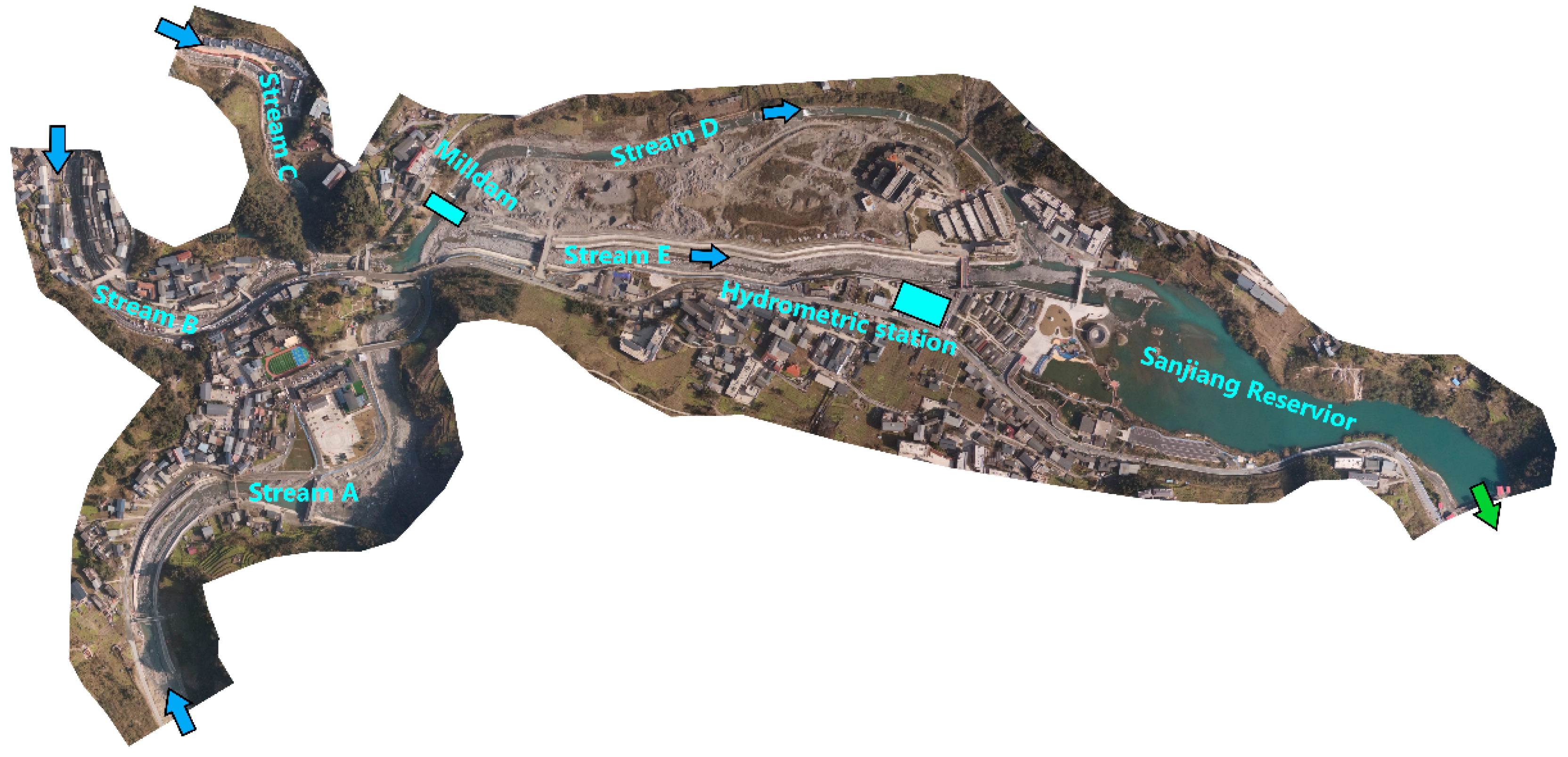
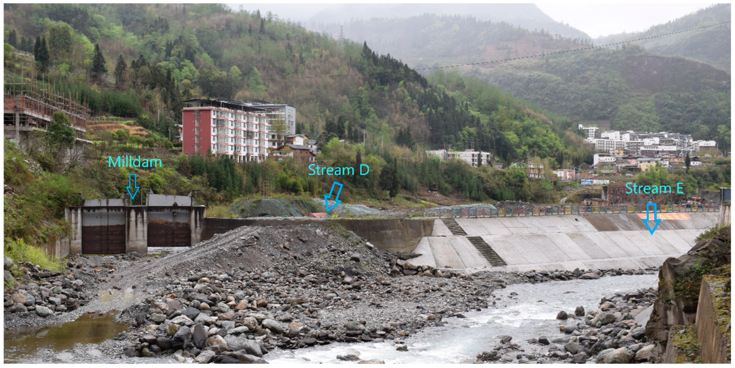
The study area covers Sanjiang Town, which lies in Sichuan Province of China. Figure 1 shows the satellite image of Sanjiang Town. The town lies at the confluence of three streams, A, B, and C. Firstly, stream B meets stream C at the upper part of the town, then they both join stream A. The distance between the two junctions is about 100 m. Right after the confluence, stream A is further divided into streams D and E. For stream D, there is a milldam near the bifurcation, and the milldam can discharge part of the flash flood through stream D. Stream E has twice the width of stream D, and releases most of the flood. Streams D and E meet again at the Sanjiang reservoir. The central bar surrounded by streams D and E is the major developing part of the town in recent years. At the end of stream E, a hydrometric station collects hydraulic data during the floods. An overflow dam lies at the end of the Sanjiang reservoir, and gates of the dam are all opened to discharge floods.
3. Methodology
In this study, we adopted the depth-averaged, two-dimensional, shallow-water equations, coupled with sediment transport and bed variation equations [22], to simulate the flash flood and sediment transport during the disaster.
Continuity equation:
Momentum equation:
Equation of bed load transport:
Equation of bed deformation:
in which denotes time, means water depth, present velocity components in the x and y directions, respectively, is gravitational acceleration, is the turbulent viscosity coefficient, and in which is the sediment density, and is the water density.
where is the volumetric sediment concentration, and is the total concentration of graded sediments (kg/m3). In this study, only the bed load transport is calculated, so equals .
in which denote the density of saturated and dry bed material, respectively. The bed slope terms and friction slope terms ) are written as , , and , in the x and y directions, respectively, where is bed elevation and is Manning’s roughness coefficient.
where is the amount of bed load in a unit volume of water, is the settling velocity of bed load, is the transport capacity of bed load in a unit volume of water, in kg/m3, and is the non-equilibrium adaptation coefficient of bed load. is an empirical coefficient, is the incipient velocity of bed load, calculated by , is the dimensionless Chézy coefficient, and is the value of bed load in a unit volume, and is obtained according to .
The governing Equations (1)–(4) can be rewritten in the form:
in which
S is the source section, and is equal to the rest of the sections of each governing equation.
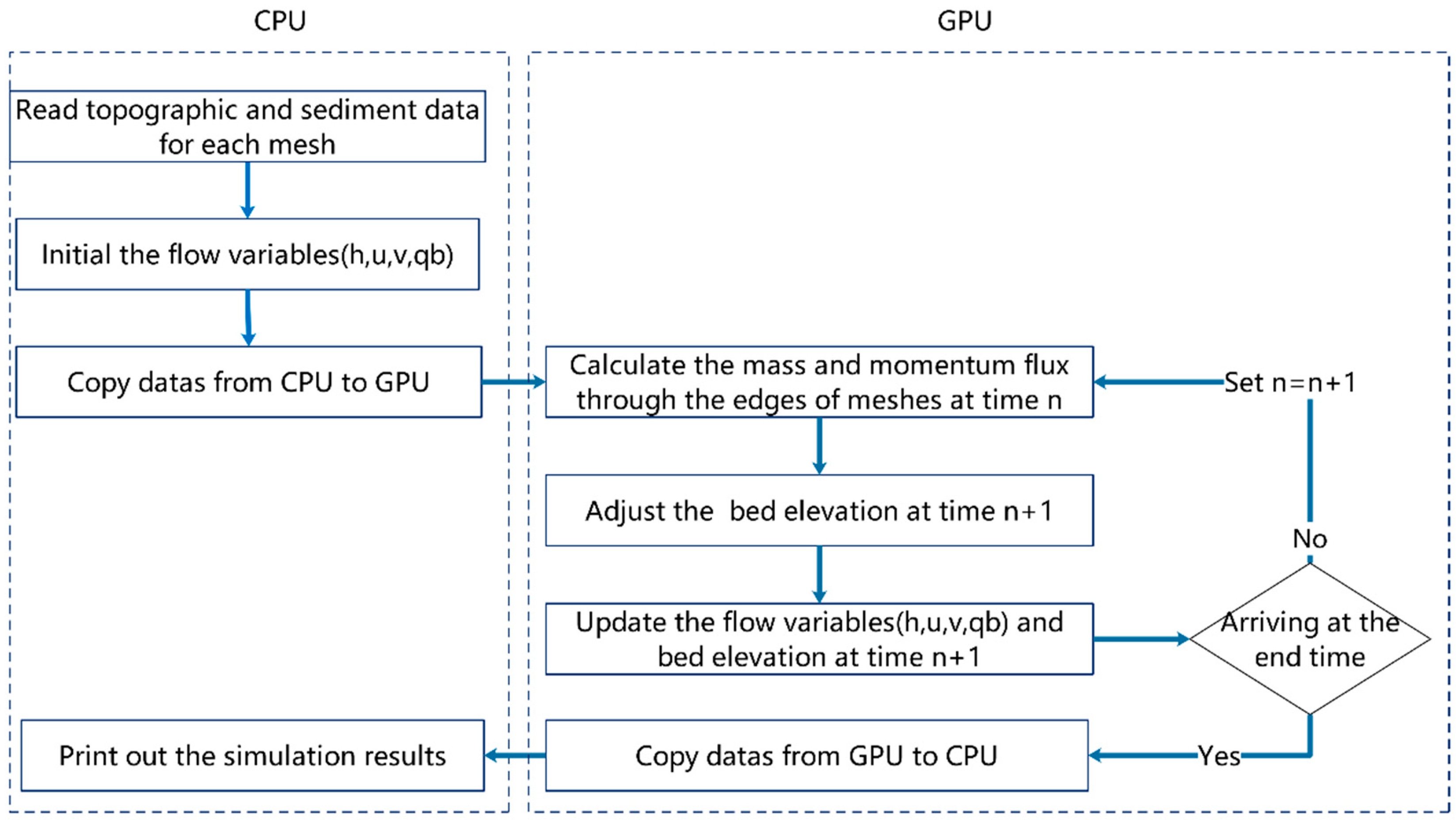
The governing equations are solved by the method of finite volume with hybrid triangular and quadrangular meshes. The variables () in each mesh are updated in a time-marching manner (Equation (11)). is the variables’ value at time n, is the variables’ value at time n + 1, and denotes the flux crossing the edges of the mesh. In order save the calculation time, a NVIDIA GeForce RTX 3050 GPU (graphics processing unit) was adopted to speed up the calculation. The flow chart of the calculation is shown in Figure 2.
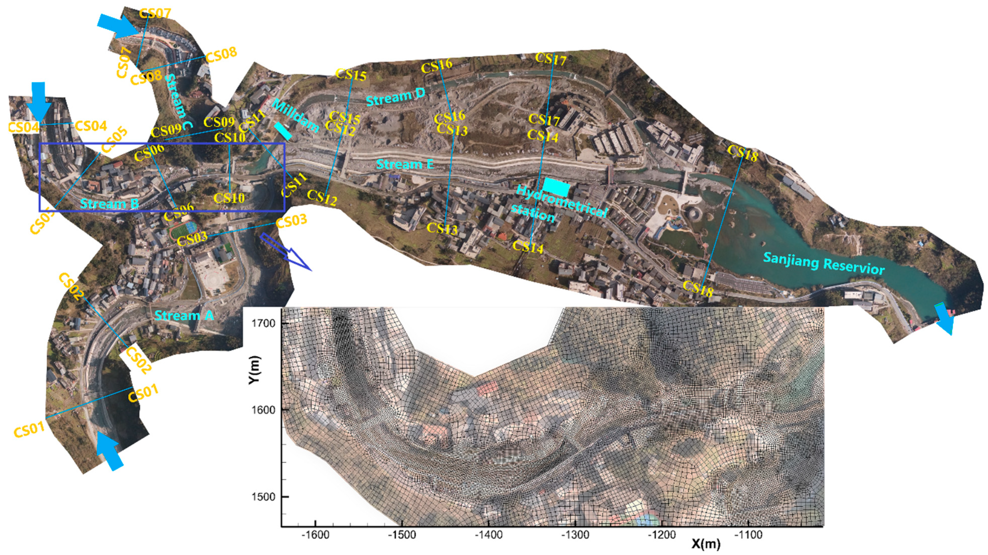
The calculation codes used in this study have been successfully used in the former studies [18,23]. The simulation region covers most parts of Sanjiang Town, and the number of simulation meshes is about 110,000. In order to capture the flash flood propagation accurately with a moderate quantity of mesh, a non-uniform (triangular and quadrangular hybrid) mesh is adopted. The size is about 2.0 m in regions near the stream channel and bank, and about 5.0 m in regions far from the streams (Figure 3).
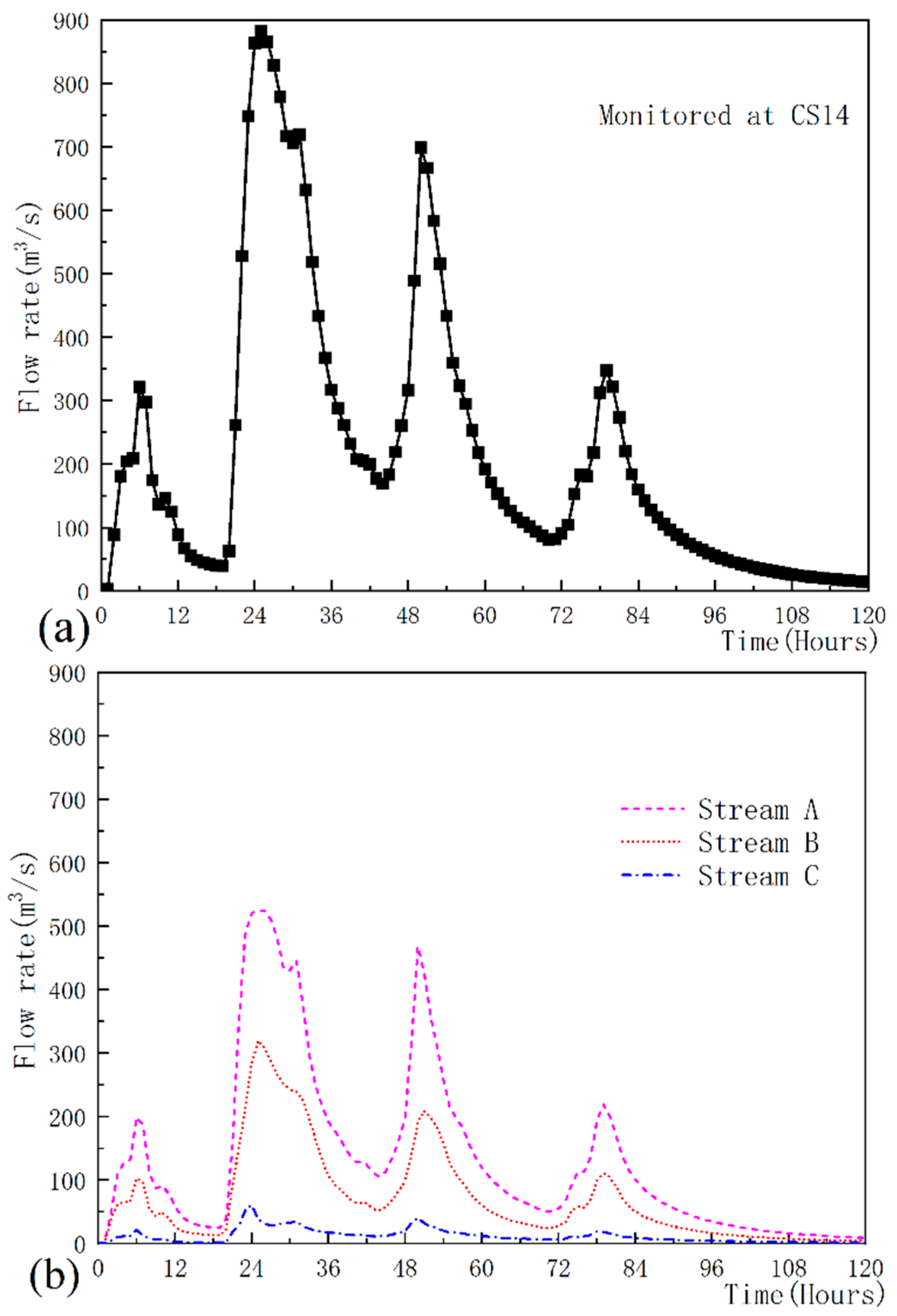
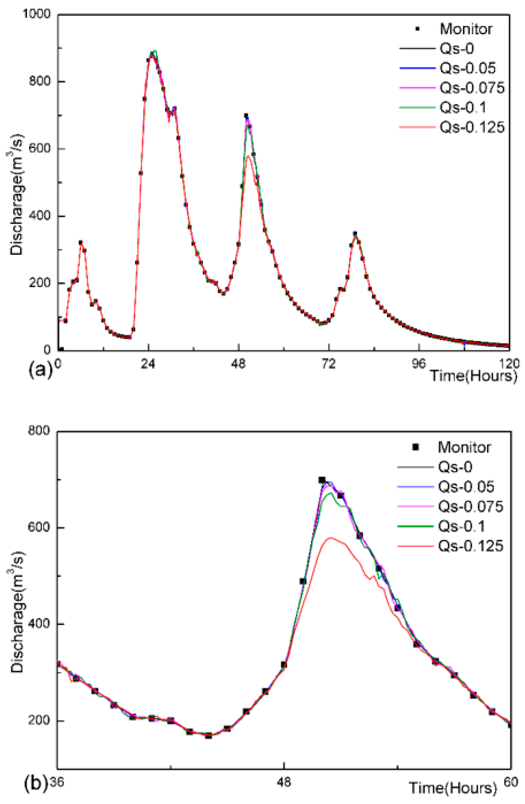
We collected high-resolution (5.0 m) DEM (digital elevation model) data (Figure 1) after the flash flood in 2019, and the flow rates of stream E (Qt(CS14)) at the hydrometric station of Sanjiang Town. The flow rates at the hydrometric station were gauged at an interval of 20 min. The flash flood lasted about 120 h (from 20 to 24 August in 2019). The 120 h-long flash flood can be divided into four stages, and each of them has one discharge peak (Figure 4a, stage 1, 2, 3, and 4, respectively). We deduced the discharge of streams A (), B (), and C () based on their upstream catchment area (Figure 4b). For example, since the milldam in stream D was closed during the flood, the total discharge of streams A, B, and C should be equal to the discharge at CS14. Supposing the catchment areas of streams A, B, and C are , respectively, and the total area of them , then = Qt, = Qt, and = Qt, respectively. All these data contribute to the numerical inversion of the flash flood.
In this study, the roughness of the bed was set with the Manning’s roughness, , of 0.025, which is suggested by hydraulics manuals [24] and verified by our former studies [18]. The bed elevations at each mesh were initiated by interpolating from the high-resolution terrain data, and updated by the simulation codes at each timestep based on Equation (5). In order to study the unsteady process of the flash flood, hydraulic data of 18 cross-sections (Figure 3) were saved at every timestep, and data of the full simulation region were saved at every 100 timesteps during the calculation.
The inlet discharges for streams A, B, and C were consistent with the deduced rate curves in Figure 4b, and flow rate of the outlet boundary was automatically calculated according to the empirical formula for weir flow. The formula is , in which = discharge, = discharge coefficient, about 0.502, = number of gates opened, = width of each gate, and = the difference between water level and elevation of the weir top. Once the discharge is calculated, the velocity at the outlet is set based on the discharge.
The milldam was closed during the flash flood in 2019 (Figure 5), and released little water to stream D. The water in streams A, B, C, and E performs as the confluence flow, but the flow will move as bifurcation flow when the milldam is open. Therefore, in order to investigate the impact of the milldam on the flash flood, scenarios with both a closed and an opened milldam were simulated in this study.
As the sediment characteristics were not monitored by the hydrometric station during the flash flood disaster, it is difficult to figure out the amount of bed load at inlet boundaries of streams A, B, and C. We assumed the inlet sediment concentrations with different percentages of transport capacity of bed load at the inlets. Transport capacity will change with velocity and depth. For example, if the transport capacity of bed load at the inlets at time A is , Qs-0.05 means the inlet sediment concentration is set as 100 × 0.05 = at time A, and Qs-0 means the inlet sediment concentration is zero all the time. For the diameters of sediment, we collected some sediment of the river bed after the flash flood in 2019, and obtained a median size of 0.02 m. The flow conditions for the simulation scenarios are listed in Table 1.
4. Results
4.1. Model Calibration
The purpose of this section is to figure out the scenario which best fits the monitored data. We analyzed the simulation results of the first five scenarios in Table 1. In these scenarios, the milldam in stream D was closed during the flood.
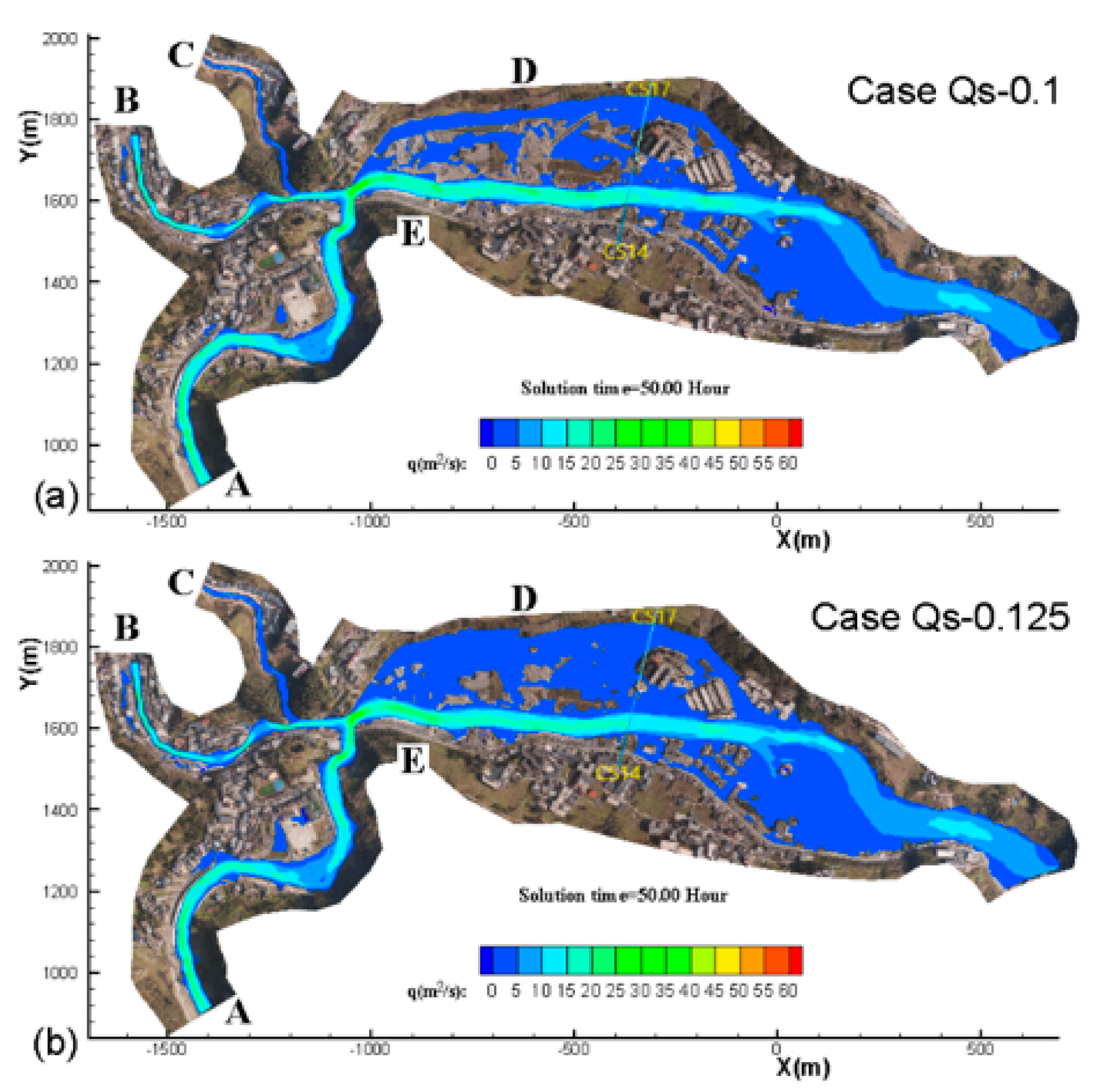
Figure 6a shows the simulated and monitored discharge profiles at CS14, and Figure 6b presents a detailed view of stage 3. It can be seen that the simulated discharge profile agrees well with the monitored data at CS14, except for that of case Qs-0.125 in stage 3. Figure 7 shows the distribution of unit width flux of cases Qs-0.125 and Qs-0.1. The flooded area of case Qs-0.125 was a bit larger than that of case Qs-0.1, and some flow travelled downstream through CS17 instead of CS14, which contributed to the bigger difference in Figure 6b.
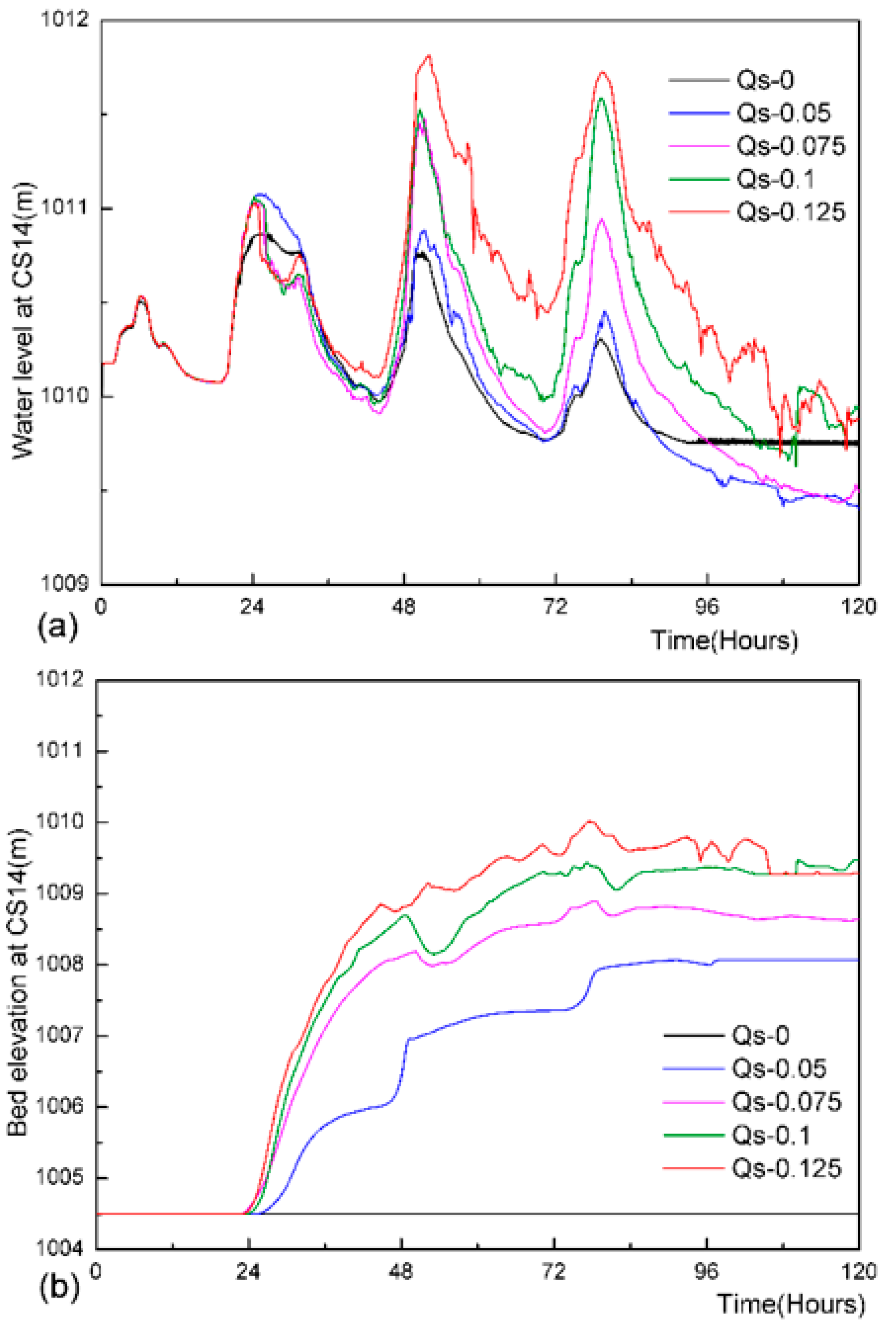
Figure 8a shows the simulated water level of each scenario. For cases Qs-0 and Qs-0.05, the maximum level occurred in stage 2 of the flood, while for cases Qs-0.075, Qs-0.1, and Qs-0.125, the maximum level occurred in stage 3. Figure 8b shows the simulated bed elevation of each scenario. The bed elevation increased rapidly in flood stages 2 and 3, and the larger the inlet sediment concentration, the more the bed elevation increased. The lifted bed elevation further contributed to the occurrence time of the maximum level being delayed from flood stage 2 to 3. The sediment deposition can change the amplitude and occurrence time of the peak level.
According to the analysis above, the discharge curves were nearly coincident with each other among the first four simulation scenarios. However, water level and bed elevation were much different from each other for cases with different inlet sediment concentrations. The different water level and bed elevation further impacted the flooded area during the flood. Based on the field investigation carried out right after the flash flood in 2019, the simulation results of case Qs-0.1 fit better concerning the flood marks, final bed elevation, flood area, etc. Therefore, we used the 10% of transport capacity (Qs-0.1) as the inlet sediment concentration.
4.2. Flash Flood in Confluence Streams (Case Qs-0.1)
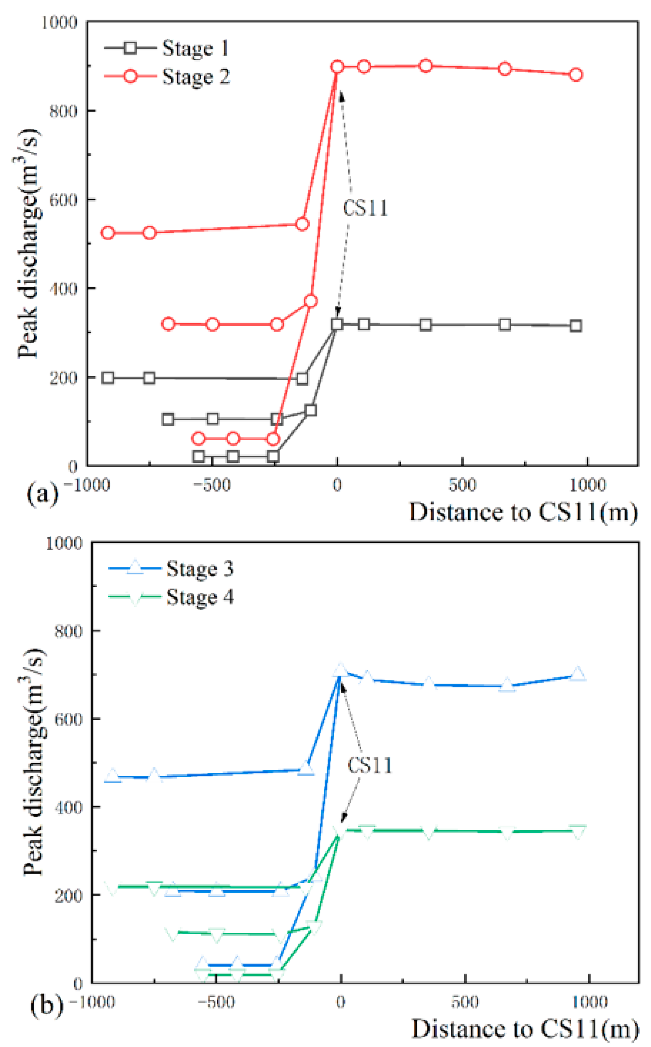
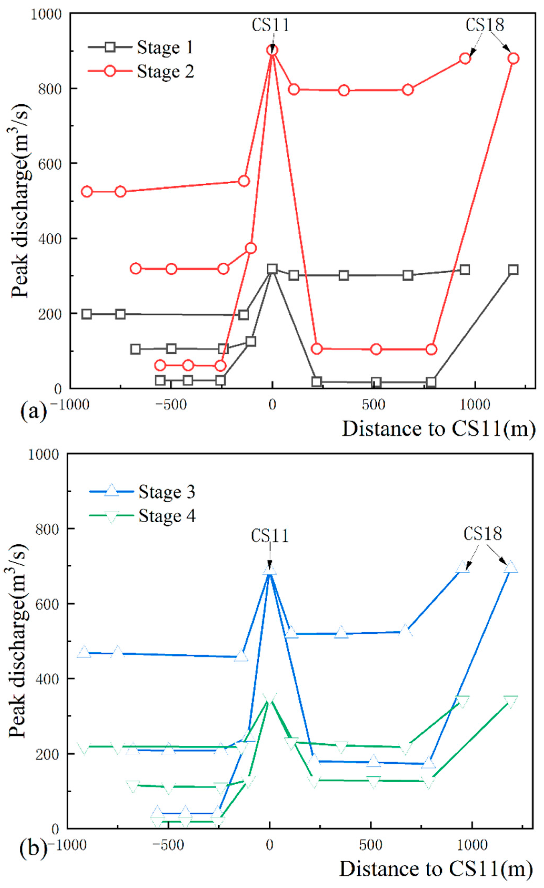
As the gates of the milldam were closed in this case, all of the flow coming from streams A, B, and C went to the reservoir through stream E. Figure 9 presents the peak discharge along the streams. In the four stages of the flash flood, the peak discharges increased rapidly at CS11, and showed little change at other parts of the streams.
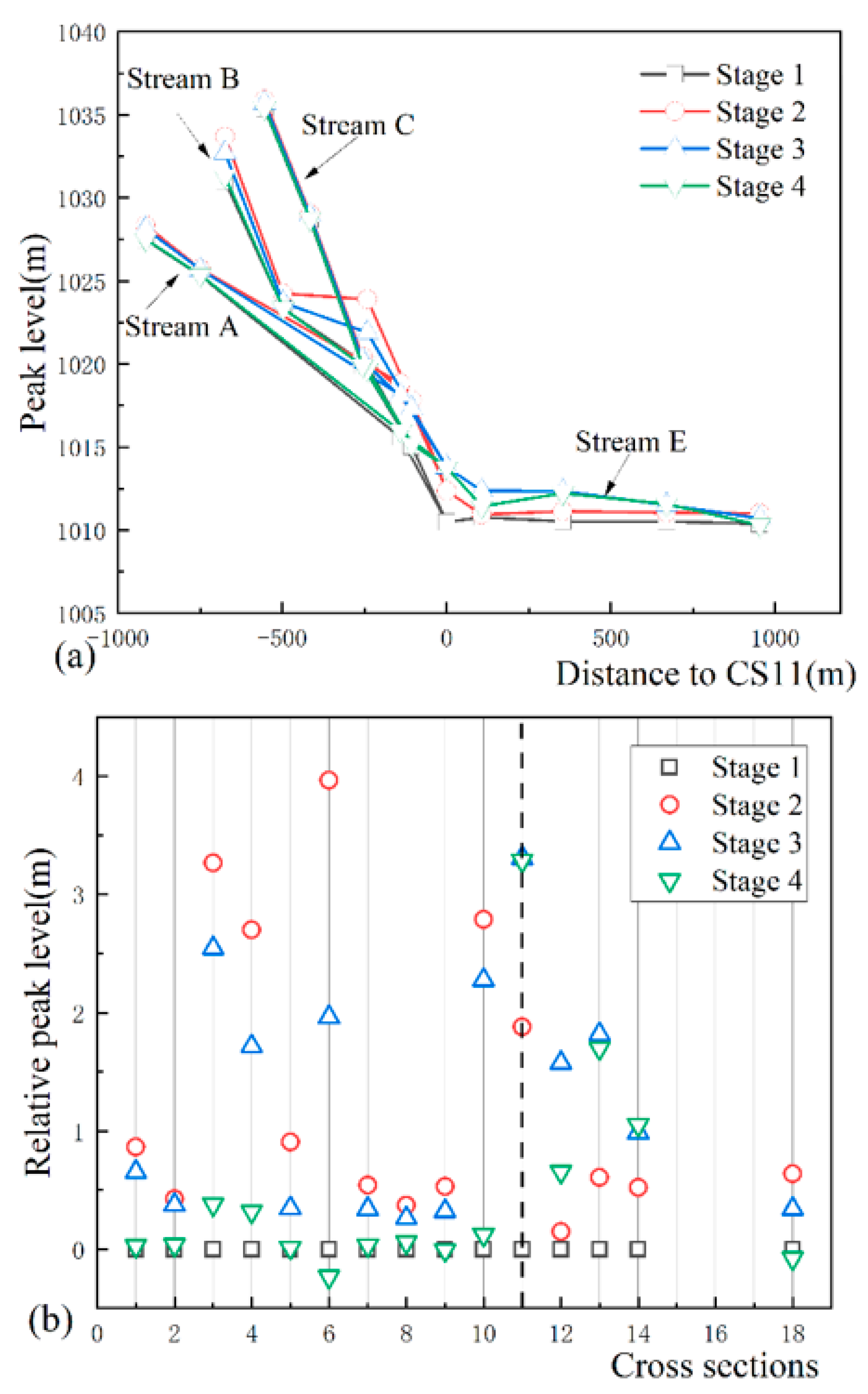
Figure 10a shows the peak level at each cross-section. The water level dropped sharply along the channel of streams A, B, and C, with a minimum slope of 2.5%. On the contrary, in stream E, the peak water level slowly decreased along the channel, and the slope was about 0.3%. Once again, this proves that the town lies in the transition region from a steep channel to a gentle slope.
Peak water levels were generally coincident with the flood marks obtained by field investigations, and it was difficult to compare them as the slope was steep (Figure 10a). Figure 10b presents the relative peak water level at all the cross-sections. The relative peak water level was obtained by subtracting the peak water level of each flood stage from that of stage 1, so the relative peak water levels of stage 1 were all zero. For cross-sections in streams A, B, and C, the maximum level occurred in stage 2, in which the maximum peak discharge existed. However, for cross-sections in stream E, the maximum level occurred in stage 3 of the flood. The bed elevation in stage 3 was much higher than that of stage 2, and the deposition lifted the water to a higher level with a relatively smaller discharge (Figure 8).
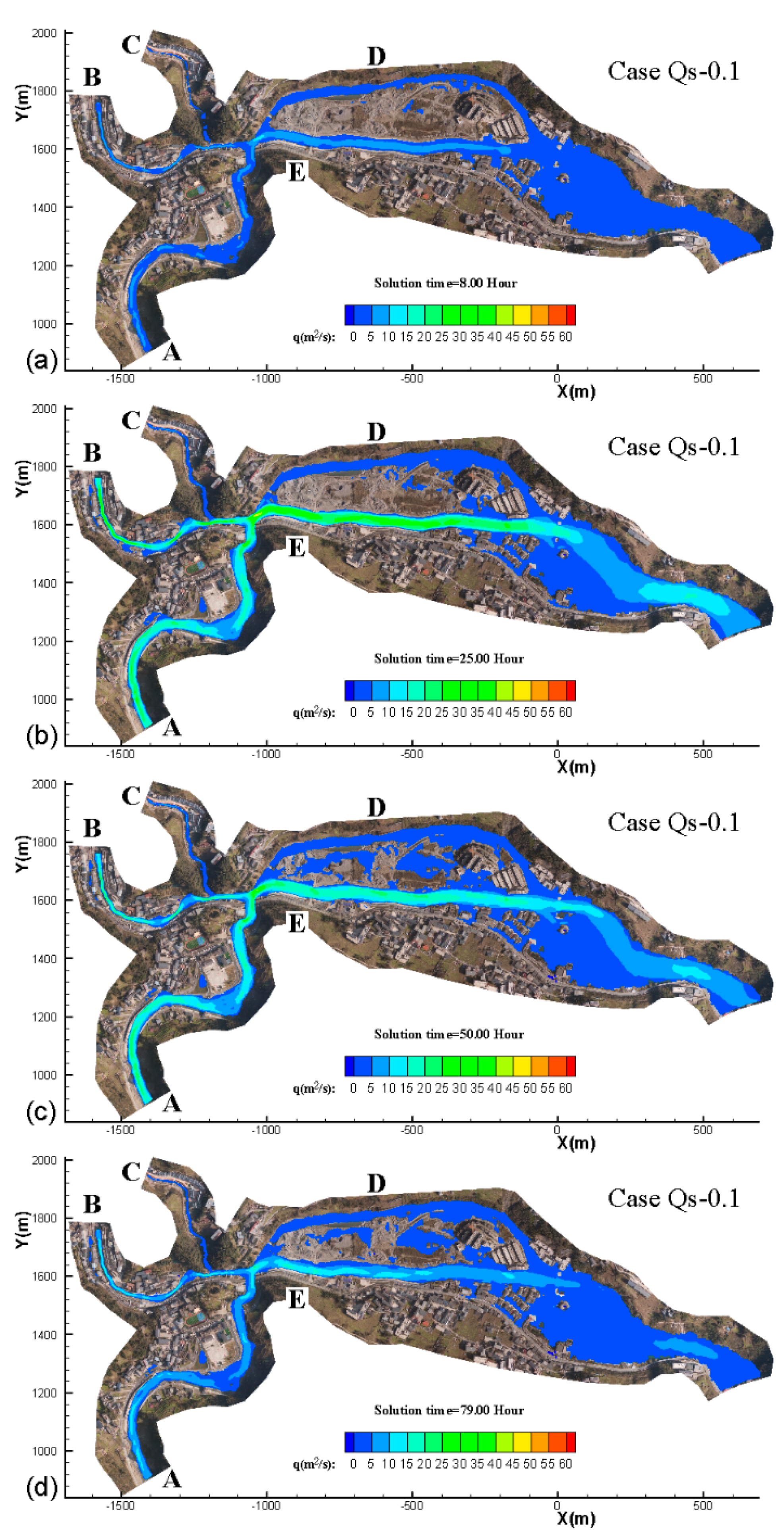
For a better understanding of the flow properties along the streams, we adopted the unit width flux to analyze the main flow variation. As the unit width flux, , is equal to the product of depth and velocity magnitude, regions with larger denote more flow passing through. Figure 11 shows the distribution of unit width flux () at the four stages of the flood. Since the milldam was closed, the main flow came from streams A and B, and went to the reservoir only through stream E.
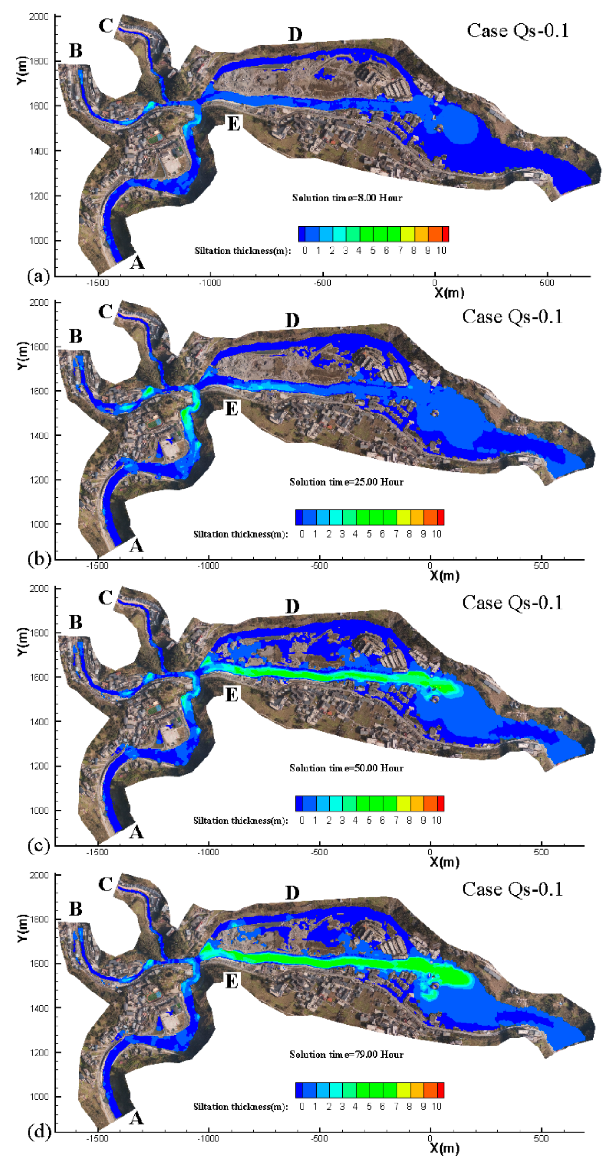
Siltation thickness denotes the differences between bed elevation at any time and that of the initial time. The larger the thickness, the more sediments deposited there. Figure 12 presents the distribution of siltation thickness at the four stages of the flood. Sediments deposited mainly at the confluence region of streams A and B in stages 1 and 2, while the main siltation region shifted to stream E in stages 3 and 4. Meanwhile, the siltation thickness in streams A and B became thinner in stages 3 and 4, which explains the finding in the field investigation whereby the flood marks were much higher but the elevation of sediments was much lower in stream A. In stages 1 and 2, the water level in streams A and B was higher due to the larger discharge and higher bed elevation, while in stages 3 and 4, the water level in streams A and B was lower due to the smaller discharge and lower bed elevation, due to erosion. After the flood, only the final bed elevation and flood marks could be measured.
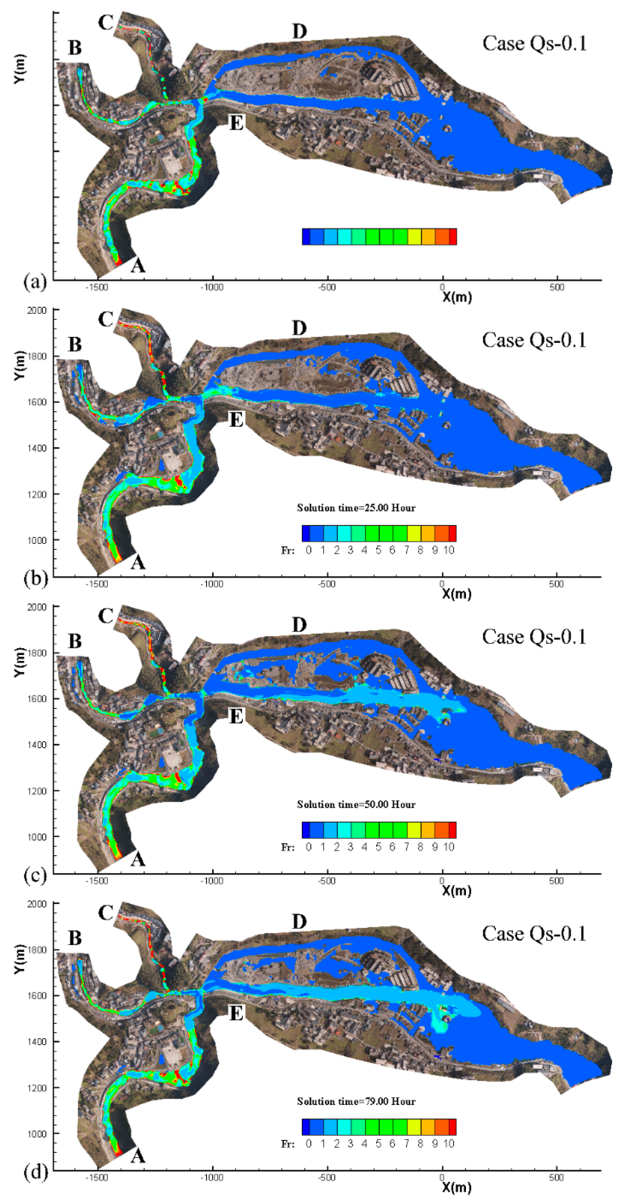
Figure 13 shows the distribution of the Froude number (Fr) at the four stages of the flood. The Froude number is defined as the velocity magnitude divided by water depth (sqrt(u ^ 2 + u ^ 2)/h). If Fr > 1, the flow is subcritical, if Fr > 1, the flow is supercritical, and if Fr = 1, the flow is critical. For streams A, B, and C, the Froude number of most regions was larger than 3 in the four flood stages, while for stream E, the flow was subcritical in stages 1 and 2, and supercritical in stages 3 and 4. There is little siltation at places with a larger Froude number. On the contrary, for stream E, the regions with a larger Froude number were nearly coincident with those of higher sediment thickness (Figure 12). The highly raised bed decreased the water depth and increased the Froude number.
4.3. Flash Flood in Streams with Bifurcation (Case Qs-0.1-Bifurcation)
As the gates of the milldam were open in this case (Qs-0.1-bifurcation), all of the flow coming from streams A, B, and C travelled to the reservoir through both stream D and stream E. Figure 14 presents the peak discharge along the streams. The peak discharge increased rapidly at CS11 and CS18 due to the combination of flows, decreased sharply after CS11, and showed little change at other parts of the stream.
Figure 15 shows the peak level at each cross-section. The water level varied in a similar way to that in Figure 10. The maximum water level of streams D and E occurred in flood stage 3 (the second largest discharge stage), while the maximum water level of streams A, B, and C occurred in flood stage 2 (the largest discharge stage).
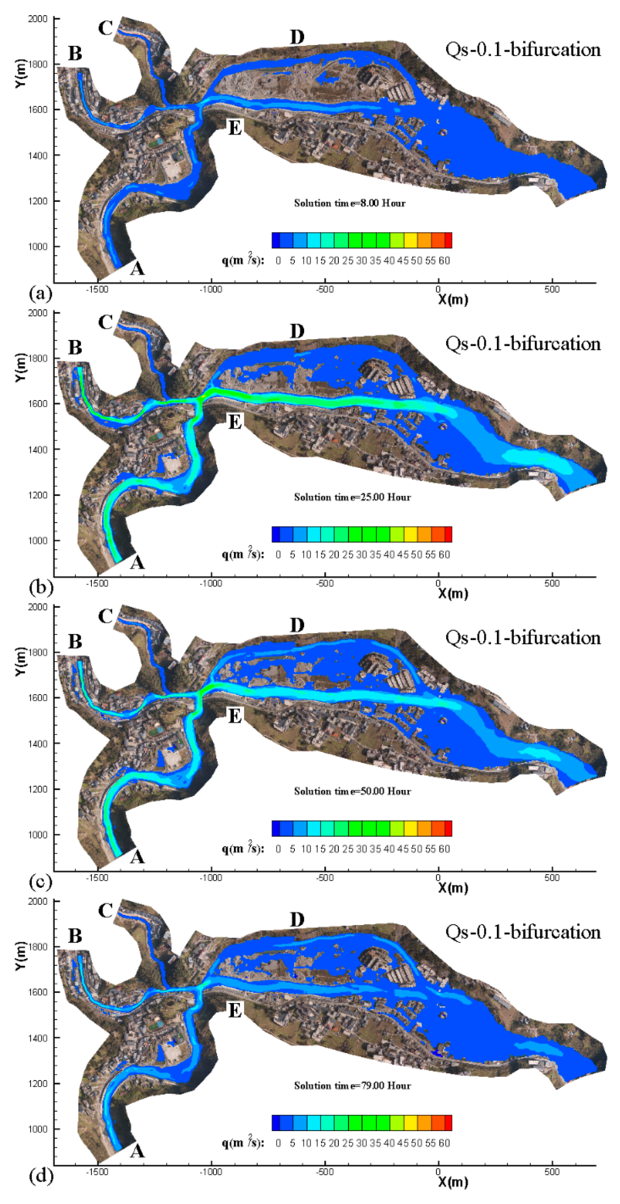
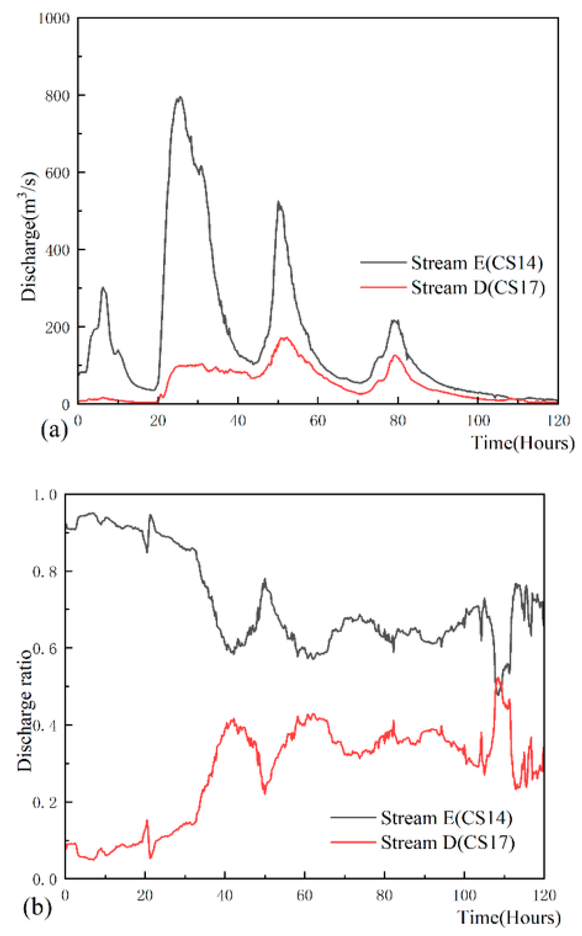
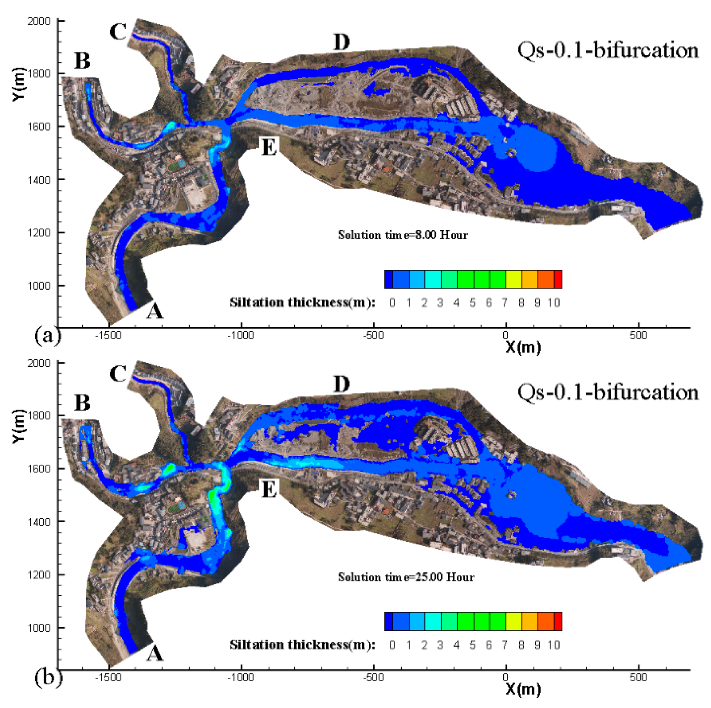
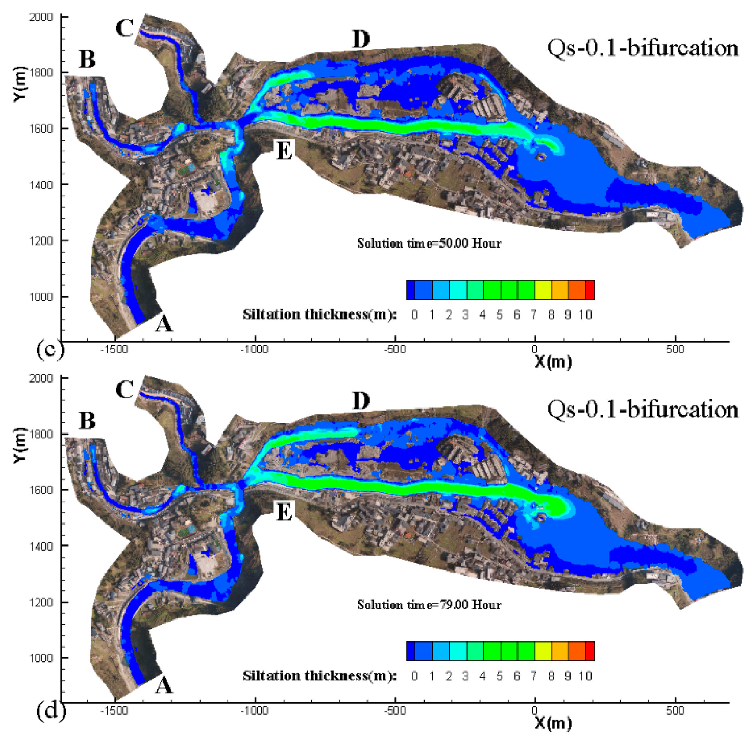
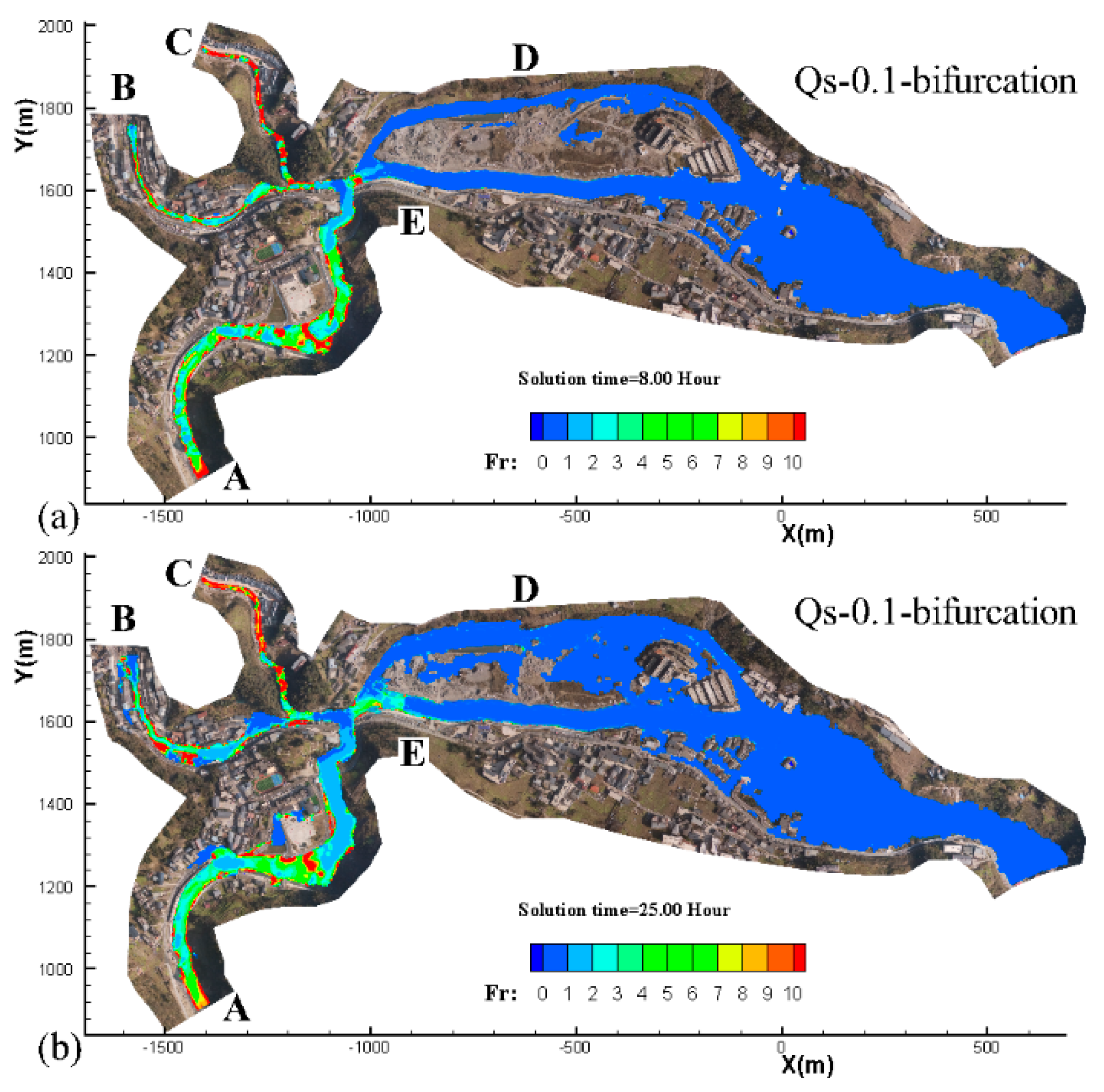
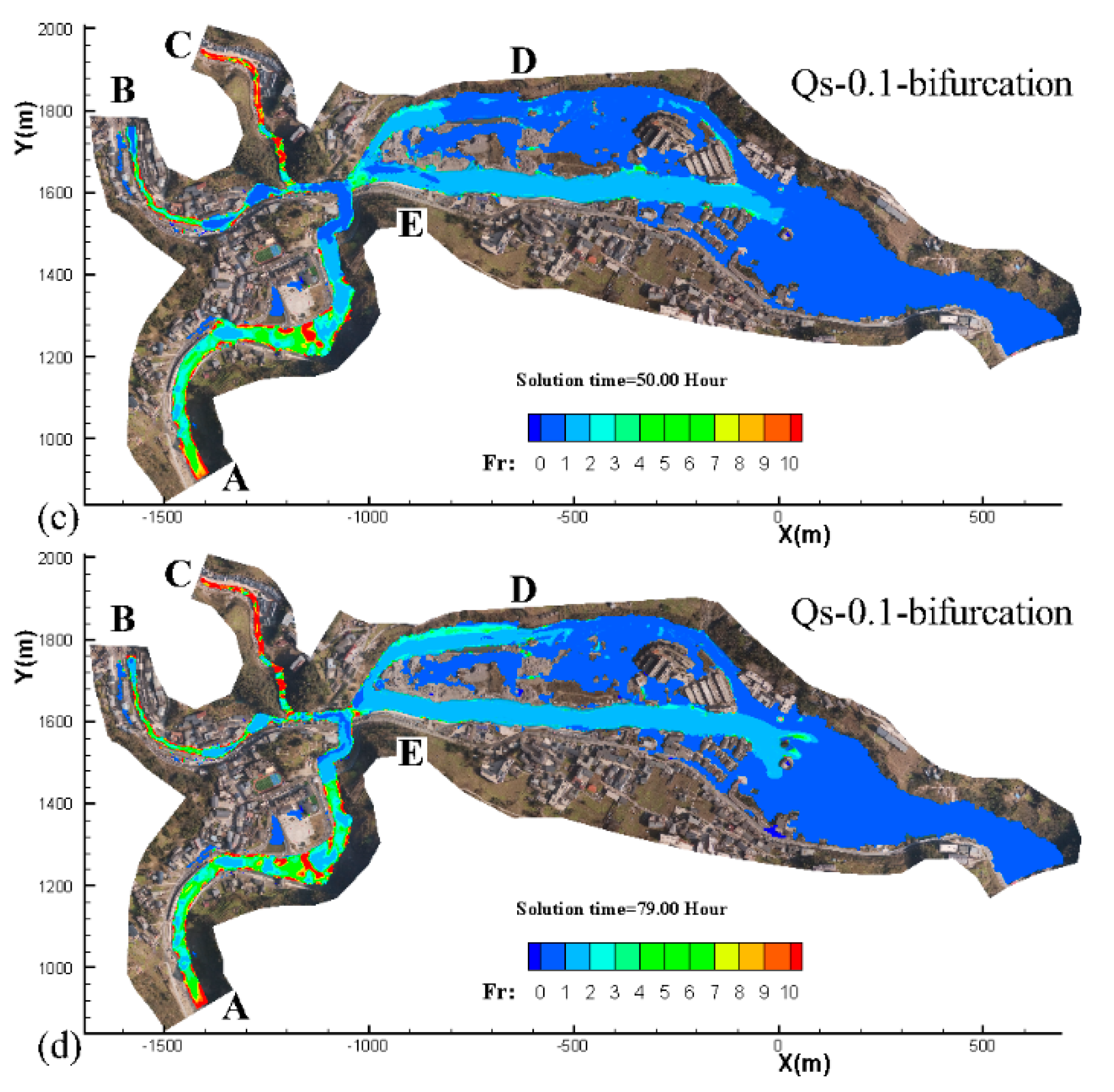
Figure 16 shows the distribution of unit width flux (q) at the four stages of the flood. The main flow came from streams A and B, and travelled to the reservoir through stream E in stages 1 and 2, while more and more flow travelled to the reservoir via stream D in stages 3 and 4. Figure 17 presents the flow rates and flow rate ratios of streams D and E. In stages 1 and 2 (before 30 h), the flow rate ratio of stream D was about 0.1, while in stages 3 and 4, the flow rate ratio of stream D increased to around 0.3. Figure 18 presents the distribution of siltation thickness at the four stages of the flood as the milldam was open. Sediments deposited mainly at the confluence region of streams A, B, and C in stages 1 and 2. The siltation region shifted to streams D and E in stages 3 and 4, and siltation in stream E increased much quicker than that in stream D. The uplifted bed of stream E pushed more water to stream D. For the distribution of Froude numbers in Figure 19, supercritical regions were still coincident with places of thick sediment deposition in streams D and E, and with little sediment deposits at places with a higher Froude number in streams A, B, and C.
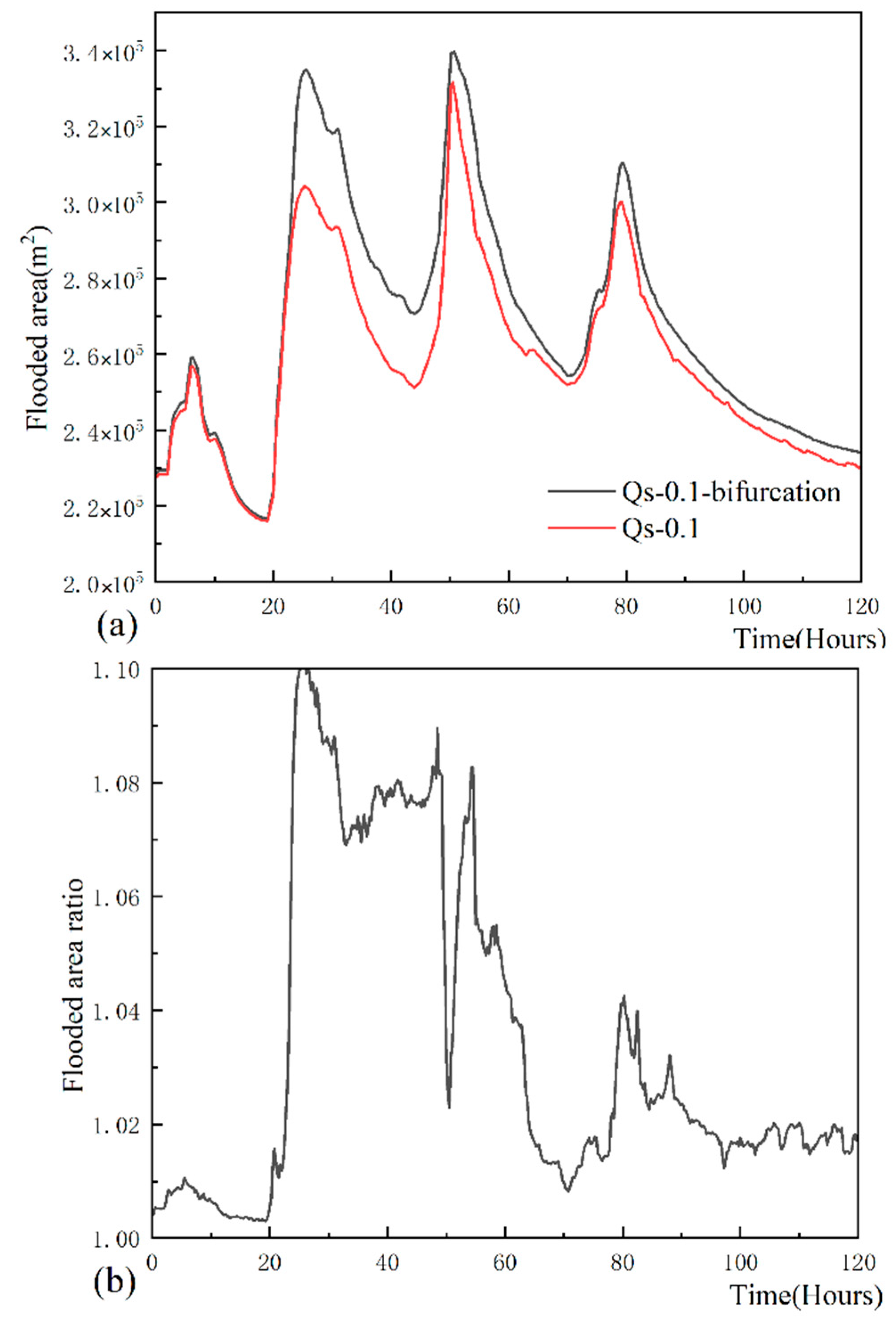
Figure 20 shows the flooded area of cases Qs-0.1 and Qs-0.1-bifurcation. Among all the four stages of the flood, the flooded area of case Qs-0.1-bifurcation was larger than that of case Qs-0.1. The flooded area ratio between case Qs-0.1-bifurcation and case Qs-0.1 is shown in Figure 20b, and the ratio had a maximum of 1.1. From the point of view of reducing the flooded area, it is better to keep the milldam closed during the flood.
5. Discussion
5.1. Boundary Conditions for the Numerical Inversion of Flash Flood
In this study, we adopted the two-dimensional shallow-water models coupled with sediment transport models to analyze the flash flood that occurred in Sanjiang Town in 2019. On most occasions, flash floods occur in a region with limited monitoring facilities. It is difficult to accurately set the boundaries for flash flood simulations. Usually, the elevation of the bed form, the grade curve of sediment, and flood marks can be measured after the flood disaster. However, the time-discharge curve, the inlet sediment concentration, and the outlet level are rather difficult to estimate. Luckily, we obtained the monitored discharge curves from the hydrometric station near Sanjiang Town, and deduced the discharge for streams A, B, and C by their upstream catchment areas. For the inlet boundary, we made assumptions with a series of sediment concentrations, and used the sediment concentration that best fit the field investigation data. Theoretically, the method is more accurate than those using a constant inlet sediment concentration, although it is still not certain that the sediment concentration is accurate due to the complexity of sediment transport. The method of evaluating the boundaries in this paper is helpful for the numerical analysis of other flash flood disasters, and hydrological models coupled with hydrodynamic models may be taken into account if the discharge curve cannot be directly obtained [2].
Furthermore, the quantitative simulation results are still helpful for taking measures against the flood. For example, keeping the milldam closed can minimize the flooding area.
5.2. Impact of Sediment on Flash Flood in Stream Confluence and Bifurcation
Flash flood wave enlargement is common in flash flood propagation, and it is usually caused by the sediment intrusion and bed form obstruction [18]. For sediment intrusion, the enlargement comes from the bulk effect, and the volume and density of fluid are both enlarged. For the bed form obstruction, the enlargement is rooted in the sharp change of the water level and velocity of the bed form. For example, the landslide dams, the change in the bed slope, etc., can increase or decrease the peak level and discharge.
The confluence and bifurcation are prototypes of streams. The flash flood enlargement in confluence streams is impacted not only by the bed form, such as the junction angle, elevation differences, etc., but also by the flow rate ratio of the streams [19]. In this study, as the flow rate ratio among streams A, B, and C was constant, the flash flood enlargement in confluence streams was mainly induced by the merging of inflows. Meanwhile, the flash flood enlargement in bifurcation streams is largely affected by the sediment deposition. The flow rate ratio between the two branches was changed by the uneven sedimentation of streams D and E. The adjustment in the flow rate ratio is similar to that in plain rivers, except that the variation in mountainous streams is much quicker [8].
The distinctive part of this study is that the study region lies in the transition region from a supercritical slope to a subcritical slope. The hydraulic slopes of streams D and E were flattened by the Sangjiang reservoir. Huge sediments deposited in streams D and E as the velocity was slowed down. From the point of view of reducing the flooded area, the position of Sangjiang reservoir was not well-planned considering the sediment transport mode, and it should be moved downstream, far away from Sanjiang Town.
6. Conclusions
(1) In this study, the flash flood that occurred on 20 August 2019 in Sanjiang Town was analyzed by a depth-averaged two-dimensional model. The simulation showed the flash flood process in detail, and introduced a method of evaluating the boundary conditions for the numerical inversion of flash floods.
(2) Mountainous streams with many people living nearby are usually reformed by manmade facilities, which will affect the flash flood propagation properties. In this study, the milldam in stream D could largely reduce the flooded area. The manmade facilities should be taken into account in the study of flash floods, and be properly utilized during the flood events. Furthermore, planning of reservoirs should consider the sediment transport properties, as the hydraulic slope will be flattened by the reservoir.
(3) For streams in the transition region from supercritical slope to subcritical slope, the flash flood enlargement in confluence streams is mainly induced by the combination of inflows, and the flash flood enlargement in streams with bifurcation is largely affected by the sediment deposition. Flow in the supercritical slope runs at a very fast velocity, and seldom deposits sediment in the steep channel. In the meantime, the sediment is transported to the streams with a flat hydraulic slope and deposited there. The transition region has a much larger probability of being submerged during the flood.
Author Contributions
Conceptualization, Q.Y. and X.W.; investigation, X.W.; resources, W.D.; data curation, Y.S. and S.X. All authors have read and agreed to the published version of the manuscript.
Funding
This research was funded by the National Key R&D Program of China (Grant No. 2019YFC1510703-03), the National Natural Science Foundation of China (Grant Nos. 51639007, 51979007, 51609014, and 51809107), and the Fundamental Research Funds for Central Public Welfare Research Institutes (Grant No. CKSF2021482/SL).
Institutional Review Board Statement
Not applicable.
Informed Consent Statement
Written informed consent has been obtained from the patient(s) to publish this paper.
Conflicts of Interest
The authors declare no conflict of interest.
Glossary of Terms
| time | |
| water depth | |
| bed elevation | |
| dimensionless Chézy coefficient | |
| Manning’s roughness coefficient | |
| velocity components in the x and y directions | |
| gravitational acceleration | |
| turbulent viscosity coefficient | |
| clear water density | |
| sediment density | |
| density of water-sediment mixture | |
| density of saturated bed material | |
| density of dry bed material | |
| amount of bed load in a unit volume of water | |
| value of bed load in a unit volume | |
| transport capacity of bed load in a unit volume of water | |
| non-equilibrium adaptation coefficient of bed load | |
| setting velocity of bed load | |
| volumetric sediment concentration | |
| total concentration of graded sediments (kg/) | |
| bed slope terms in the x and y directions | |
| friction slope terms in the x and y directions | |
| empirical coefficient | |
| incipient velocity of bed load | |
| source section | |
| vector of the conserved variables | |
| convective flux vectors of the flow in the x and y directions | |
| components of unit normal vector in the x and y directions |
References
- Sayama, T.; Matsumoto, K.; Kuwano, Y.; Takara, K. Application of Backpack-Mounted Mobile Mapping System and Rainfall–Runoff–Inundation Model for Flash Flood Analysis. Water 2019, 11, 963. [Google Scholar] [CrossRef] [Green Version]
- Li, W.J.; Lin, K.R.; Zhao, T.T.G.; Lan, T.; Chen, X.H.; Du, H.W.; Chen, H.Y. Risk assessment and sensitivity analysis of flash floods in ungauged basins using coupled hydrologic and hydrodynamic models. J. Hydrol. 2019, 572, 108–120. [Google Scholar] [CrossRef]
- Prasad, R.N.; Pani, P. Geo-hydrological analysis and sub watershed prioritization for flash flood risk using weighted sum model and Snyder’s synthetic unit hydrograph. Model. Earth Syst. Environ. 2017, 3, 1491–1502. [Google Scholar] [CrossRef]
- Chen, H.Y.; Cui, P.; Zhou, G.G.D.; Zhu, X.H.; Tang, J.B. Experimental study of debris flow caused by domino failures of landslide dams. Int. J. Sediment Res. 2014, 29, 414–422. [Google Scholar] [CrossRef]
- Zhou, G.G.; Cui, P.; Zhu, X.; Tang, J.; Chen, H.; Sun, Q. A preliminary study of the failure mechanisms of cascading landslide dams. Int. J. Sediment Res. 2015, 30, 223–234. [Google Scholar] [CrossRef]
- Zhang, Y.; Wang, Y.; Zhang, Y.; Luan, Q.; Liu, H. Multi-scenario flash flood hazard assessment based on rainfall–runoff modeling and flood inundation modeling: A case study. Nat. Hazards 2020, 105, 967–981. [Google Scholar] [CrossRef]
- Guan, M.F.; Carrivick, J.L.; Wright, N.G.; Sleigh, P.A.; Staines, K.E.H. Quantifying the combined effects of multiple extreme floods on river channel geometry and on flood hazards. J. Hydrol. 2016, 538, 256–268. [Google Scholar] [CrossRef]
- Liu, T.H.; Wang, Y.K.; Wang, X.K.; Duan, H.F.; Yan, X.F. Morphological environment survey and hydrodynamic modeling of a large bifurcation-confluence complex in Yangtze River, China. Sci. Total Environ. 2020, 737, 139705. [Google Scholar] [CrossRef]
- Toro, E.F. Shock Capturing Methods for Free Surface Shallow Flows; John Wiley & Sons: Chichester, UK, 2001. [Google Scholar]
- Schippa, L.; Pavan, S. Numerical modelling of catastrophic events produced by mud or debris flows. Int. J. Saf. Secur. Eng. 2011, 4, 403–422. [Google Scholar] [CrossRef]
- Yang, Q.Y.; Lu, W.Z.; Zhou, S.F.; Wang, X.K. Impact of dissipation and dispersion terms on simulations of open-channel confluence flow using two-dimensional depth averaged model. Hydrol. Process. 2014, 28, 3230–3240. [Google Scholar] [CrossRef]
- Yoshioka, H.; Unami, K.; Fujihara, M. A dual finite volume method scheme for catastrophic flash floods in channel networks. Appl. Math. Model. 2015, 39, 205–229. [Google Scholar] [CrossRef] [Green Version]
- Hu, X.Z.; Song, L.X. Hydrodynamic modeling of flash flood in mountain watersheds based on high-performance GPU computing. Nat. Hazards 2018, 91, 567–586. [Google Scholar] [CrossRef]
- Bellos, V.; Papageorgaki, I.; Kourtis, I.; Vangelis, H.; Kalogiros, I.; Tsakiris, G. Reconstruction of a flash flood event using a 2D hydrodynamic model under spatial and temporal variability of storm. Nat. Hazards 2020, 101, 711–726. [Google Scholar] [CrossRef]
- Contreras, M.T.; Escauriaza, C. Modeling the effects of sediment concentration on the propagation of flash floods in an Andean watershed. Nat. Hazards Earth Syst. 2020, 20, 221–241. [Google Scholar] [CrossRef] [Green Version]
- Lorenzo-Lacruz, J.; Amengual, A.; Garcia, C.; Moran-Tejeda, E.; Homar, V.; Maimo-Far, A.; Hermoso, A.; Ramis, C.; Romero, R. Hydro-meteorological reconstruction and geomorphological impact assessment of the October 2018 catastrophic flash flood at Sant Llorenc, Mallorca (Spain). Nat. Hazards Earth Syst. Sci. 2019, 19, 2597–2617. [Google Scholar] [CrossRef] [Green Version]
- Liu, W.; He, S. Dynamic simulation of a mountain disaster chain: Landslides, barrier lakes, and outburst floods. Nat. Hazards 2017, 90, 757–775. [Google Scholar] [CrossRef]
- Yang, Q.Y.; Guan, M.F.; Peng, Y.; Chen, H.Y. Numerical investigation of flash flood dynamics due to cascading failures of natural landslide dams. Eng. Geol. 2020, 276, 105765. [Google Scholar] [CrossRef]
- Wang, X.K.; Yan, X.F.; Duan, H.F.; Liu, X.N.; Huang, E. Experimental study on the influence of river flow confluences on the open channel stage–discharge relationship. Hydrol. Sci. J. 2019, 64, 2025–2039. [Google Scholar] [CrossRef]
- Chen, S.; Li, Y.; Tian, Z.; Fan, Q. On Dam-Break Flow Routing in Confluent Channels. Int. J. Environ. Res. Public Health 2019, 16, 4384. [Google Scholar] [CrossRef] [Green Version]
- Hackney, C.R.; Darby, S.E.; Parsons, D.R.; Leyland, J.; Aalto, R.; Nicholas, A.P.; Best, J.L. The influence of flow discharge variations on the morphodynamics of a diffluence-confluence unit on a large river. Earth Surf. Process. Landf. 2018, 43, 349–362. [Google Scholar] [CrossRef] [Green Version]
- Xia, J.; Lin, B.; Falconer, R.A.; Wang, G. Modelling dam-break flows over mobile beds using a 2D coupled approach. Adv. Water Resour. 2010, 33, 171–183. [Google Scholar] [CrossRef]
- Yang, Q.; Liu, T.; Zhai, J.; Wang, X. Numerical Investigation of a Flash Flood Process that Occurred in Zhongdu River, Sichuan, China. Front. Earth Sci. 2021, 9, 486. [Google Scholar] [CrossRef]
- Chaudhry, M.H. Open-Channel Hydraulics, 2nd ed.; Springer: New York, NY, USA, 2008. [Google Scholar]
Figure 1.
Satellite image of Sanjing Town, Sichuan, China.

Figure 2.
Flow chart of the calculation.

Figure 3.
Recorded cross-sections (top) and part of the calculation meshes (bottom).

Figure 4.
Monitored (a) and deduced (b) discharges of the flash flood.

Figure 5.
Image of the milldam after the flash flood in 2019.

Figure 6.
Simulated and monitored discharge profiles at CS14: (a) whole flood and (b) stage 3 of the flood.
Figure 6.
Simulated and monitored discharge profiles at CS14: (a) whole flood and (b) stage 3 of the flood.

Figure 7.
Flooded region of cases Qs-0.1 (a) and Qs-0.125 (b).

Figure 8.
Simulated water level (a) and bed elevation (b) at CS14.

Figure 9.
Peak discharge along the streams (Case Qs-0.1, (a) stage 1 and 2, (b) stage 3 and 4).

Figure 10.
Peak water level (a) and relative peak water level (b) (Case Qs-0.1).

Figure 11.
Distribution of unit width flux () at the four stages of the flood ((a) stage 1, (b) stage 2, (c) stage 3, (d) stage 4).
Figure 11.
Distribution of unit width flux () at the four stages of the flood ((a) stage 1, (b) stage 2, (c) stage 3, (d) stage 4).

Figure 12.
Distribution of siltation thickness at the four stages of the flood ((a) stage 1, (b) stage 2, (c) stage 3, (d) stage 4).
Figure 12.
Distribution of siltation thickness at the four stages of the flood ((a) stage 1, (b) stage 2, (c) stage 3, (d) stage 4).

Figure 13.
Distribution of the Froude number at the four stages of the flood ((a) stage 1, (b) stage 2, (c) stage 3, (d) stage 4).
Figure 13.
Distribution of the Froude number at the four stages of the flood ((a) stage 1, (b) stage 2, (c) stage 3, (d) stage 4).

Figure 14.
Peak discharge along the streams (Qs-0.1-bifurcation, flood (a) stage 1, stage 2. (b) stage 3, stage 4).
Figure 14.
Peak discharge along the streams (Qs-0.1-bifurcation, flood (a) stage 1, stage 2. (b) stage 3, stage 4).

Figure 15.
Peak water level (a) and relative peak water level (b) (Qs-0.1-bifurcation).

Figure 16.
Distribution of unit width flux (q) at the four stages of the flood ((a) stage 1, (b) stage 2, (c) stage 3, (d) stage 4).
Figure 16.
Distribution of unit width flux (q) at the four stages of the flood ((a) stage 1, (b) stage 2, (c) stage 3, (d) stage 4).

Figure 17.
Discharge (a) and discharge ratios (b) between streams D and E.

Figure 18.
Distribution of siltation thickness at the four stages of the flood ((a)stage 1, (b) stage 2, (c) stage 3, (d) stage 4).
Figure 18.
Distribution of siltation thickness at the four stages of the flood ((a)stage 1, (b) stage 2, (c) stage 3, (d) stage 4).


Figure 19.
Distribution of the Froude number at the four stages of the flood ((a)stage 1, (b) stage 2, (c) stage 3, (d) stage 4).
Figure 19.
Distribution of the Froude number at the four stages of the flood ((a)stage 1, (b) stage 2, (c) stage 3, (d) stage 4).


Figure 20.
Flooded area of cases Qs-0.1 (a) and Qs-0.1-bifurcation (b).


Table 1.
Flow conditions for the simulation scenarios.
| Scenarios | Inlet Discharge | Inlet Sediment Concentration | Milldam of Stream D |
|---|---|---|---|
| Case Qs-0 | Same as Figure 4b | 0 | Closed |
| Case Qs-0.05 | 0.05 × | Closed | |
| Case Qs-0.075 | 0.075 × | Closed | |
| Case Qs-0.1 | 0.1 × | Closed | |
| Case Qs-0.125 | 0.125 × | Closed | |
| Case Qs-0.1-bifurcation | 0.1 × | Open |
Publisher’s Note: MDPI stays neutral with regard to jurisdictional claims in published maps and institutional affiliations. |
© 2022 by the authors. Licensee MDPI, Basel, Switzerland. This article is an open access article distributed under the terms and conditions of the Creative Commons Attribution (CC BY) license (https://creativecommons.org/licenses/by/4.0/).
Share and Cite
MDPI and ACS Style
Yang, Q.; Wang, X.; Sun, Y.; Duan, W.; Xie, S. Numerical Investigation on a Flash Flood Disaster in Streams with Confluence and Bifurcation. Water 2022, 14, 1646. https://0-doi-org.brum.beds.ac.uk/10.3390/w14101646
AMA Style
Yang Q, Wang X, Sun Y, Duan W, Xie S. Numerical Investigation on a Flash Flood Disaster in Streams with Confluence and Bifurcation. Water. 2022; 14(10):1646. https://0-doi-org.brum.beds.ac.uk/10.3390/w14101646
Chicago/Turabian StyleYang, Qingyuan, Xiekang Wang, Yi Sun, Wengang Duan, and Shan Xie. 2022. "Numerical Investigation on a Flash Flood Disaster in Streams with Confluence and Bifurcation" Water 14, no. 10: 1646. https://0-doi-org.brum.beds.ac.uk/10.3390/w14101646
Note that from the first issue of 2016, this journal uses article numbers instead of page numbers. See further details here.