
Metropolis-Hastings Markov Chain Monte Carlo Approach to Simulate van Genuchten Model Parameters for Soil Water Retention Curve


Abstract
:1. Introduction
2. Materials and Methods
2.1. Soil Water Content under Certain Matric Potential Gradient
2.2. The van Genuchten (VG) Model
2.3. Markov Chain Monte Carlo (MCMC) Approach
2.4. Obtaining Parameters of VG Model Using the MH-MCMC Approach
- (1)
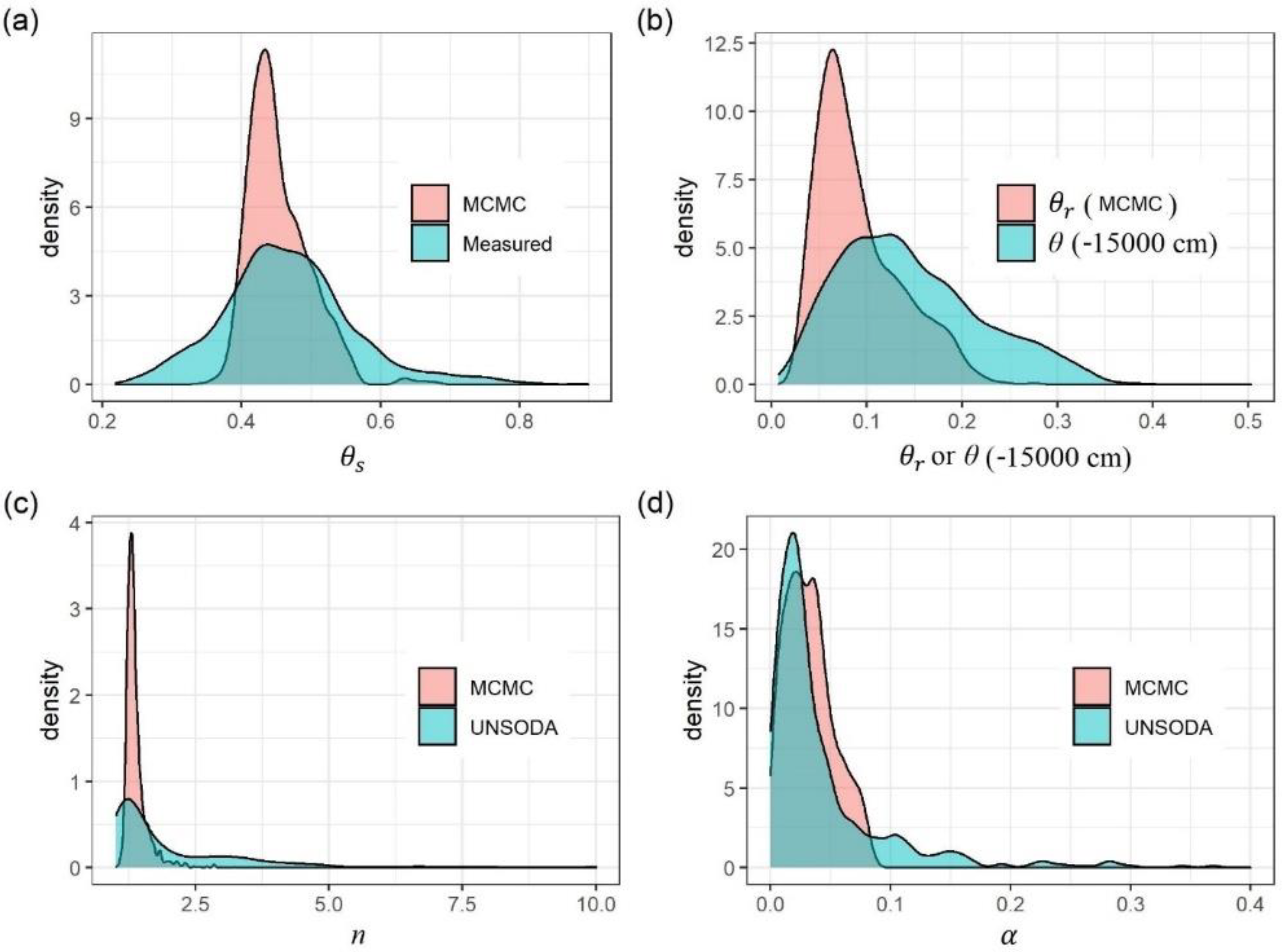
- Initiating the model parameters, as MH-MCMC is not sensitive to the initial condition, we therefore set a same values for all soil samples, i.e., set = 0.56, = 0.18, α = 0.049, and n = 1.5 as initial values for the VG model parameters.
- (2)
- Based on the model and the measured SWC under different pressure heads to get an initial estimate of and h.
- (3)
- Generating an arbitrary Markov Chain stationary distribution and its transfer matrix Q. Sample from any simple probability distribution to get the initial state value, x0.
- (4)
- Set accept rate = .
- (5)
- Sample from the conditional probability distribution , get ; sample from the uniform distribution ; if , accept , i.e., ; and otherwise, reject transformation, i.e., .
2.5. Obtaining Parameters of VG Model Using the RETC Program
2.6. Model Evaluation
3. Results
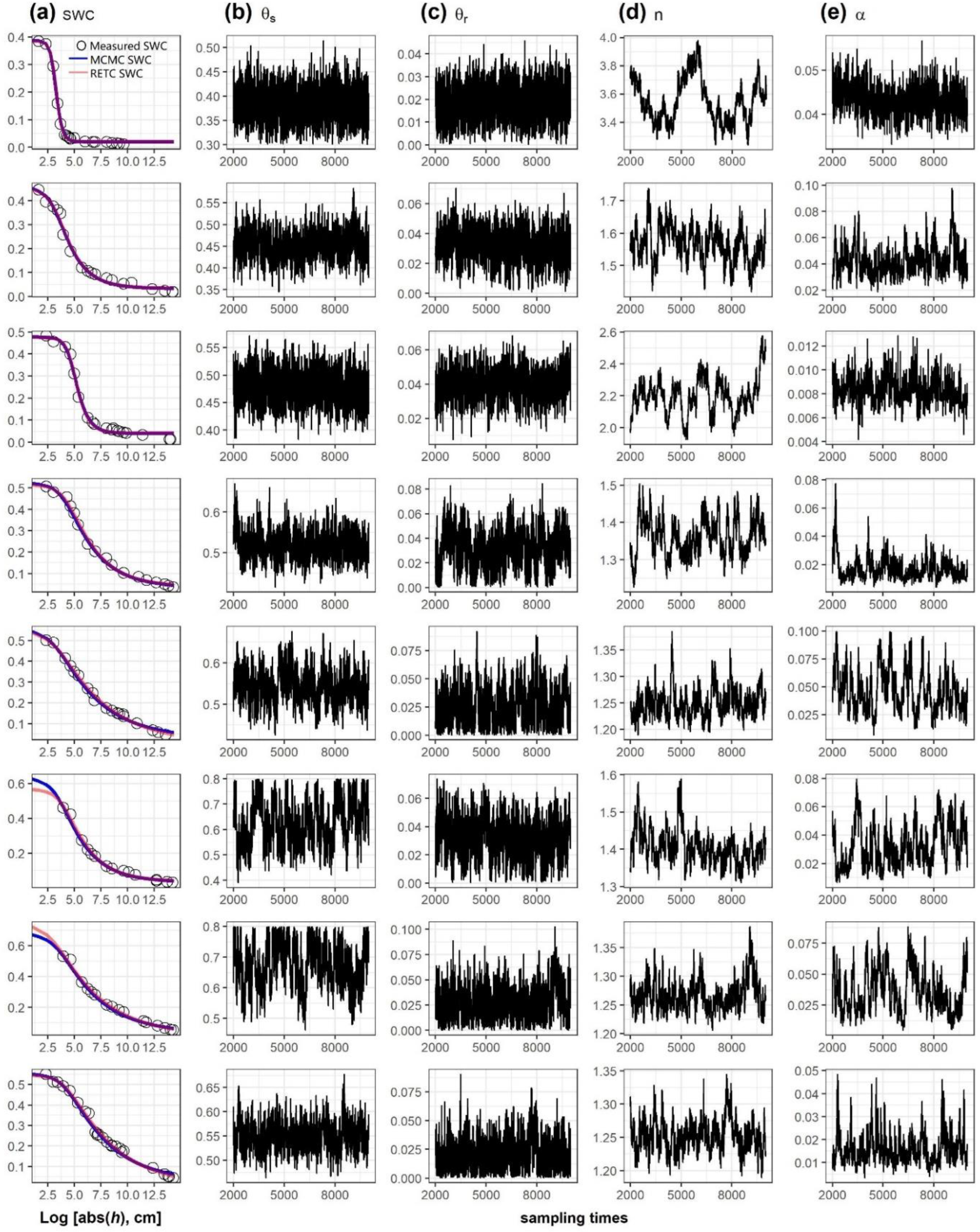
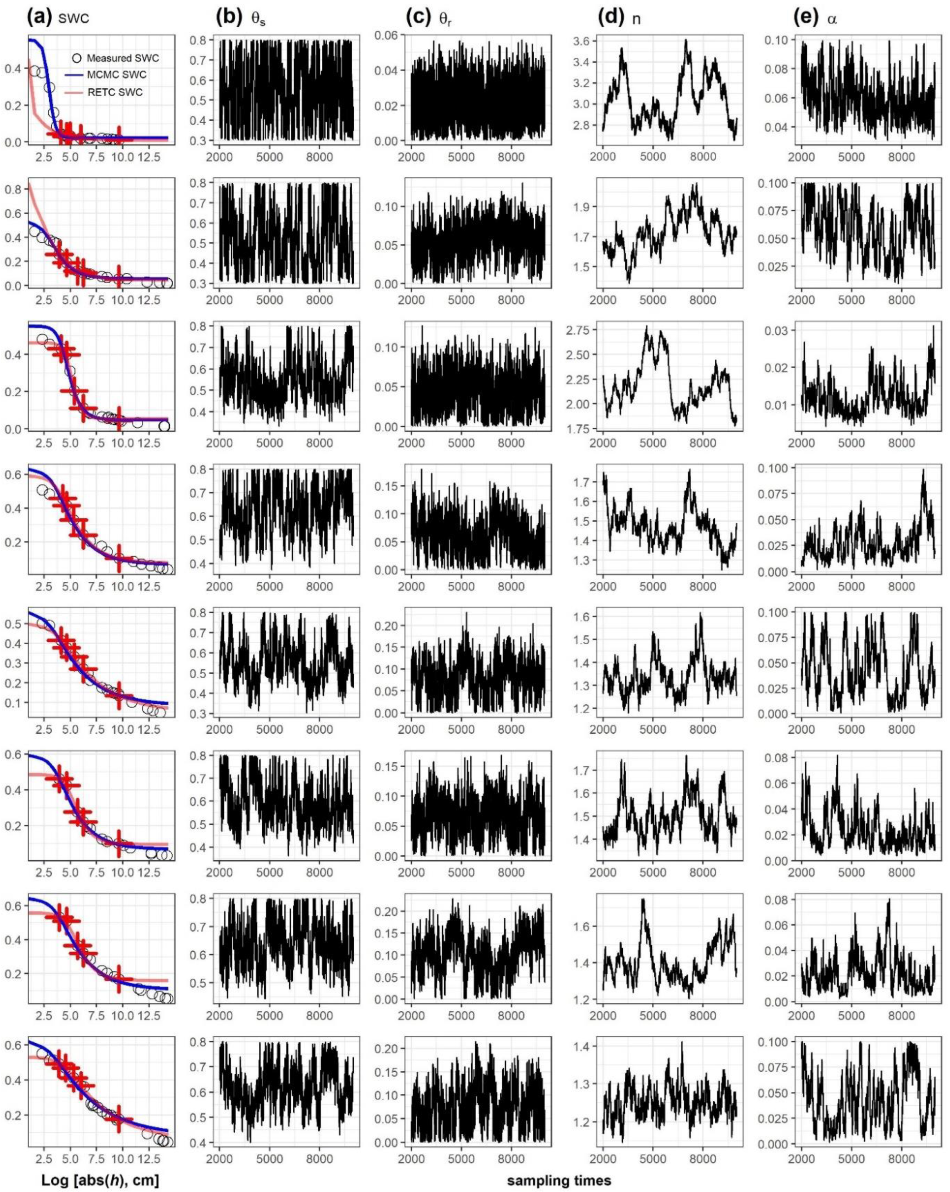
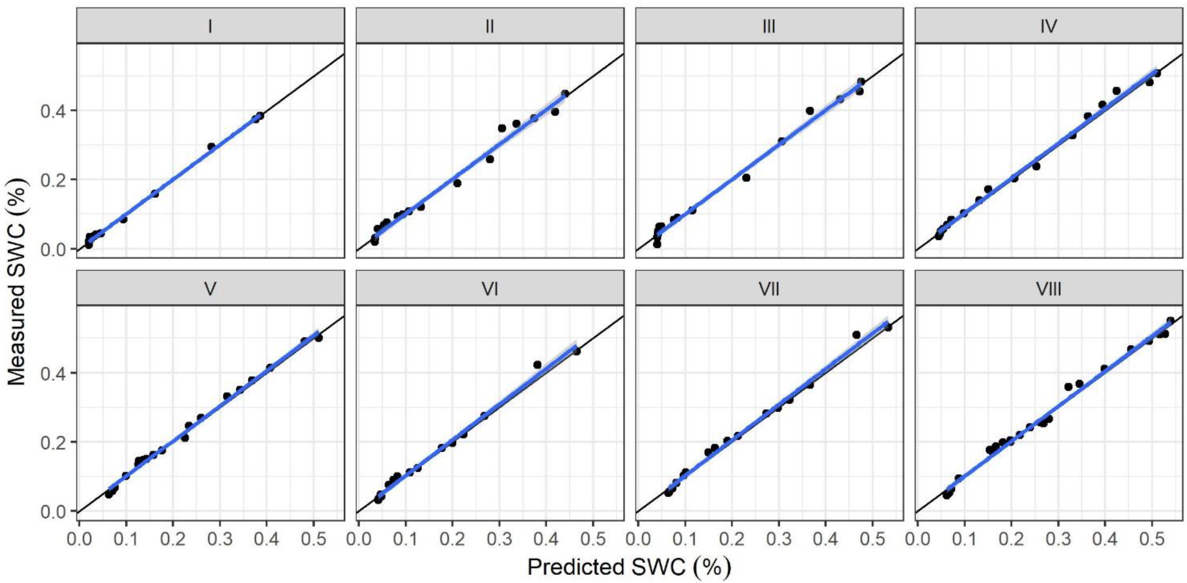
3.1. Fitted Soil Water Retention Curve by the MH-MCMC Approach and the RETC Program
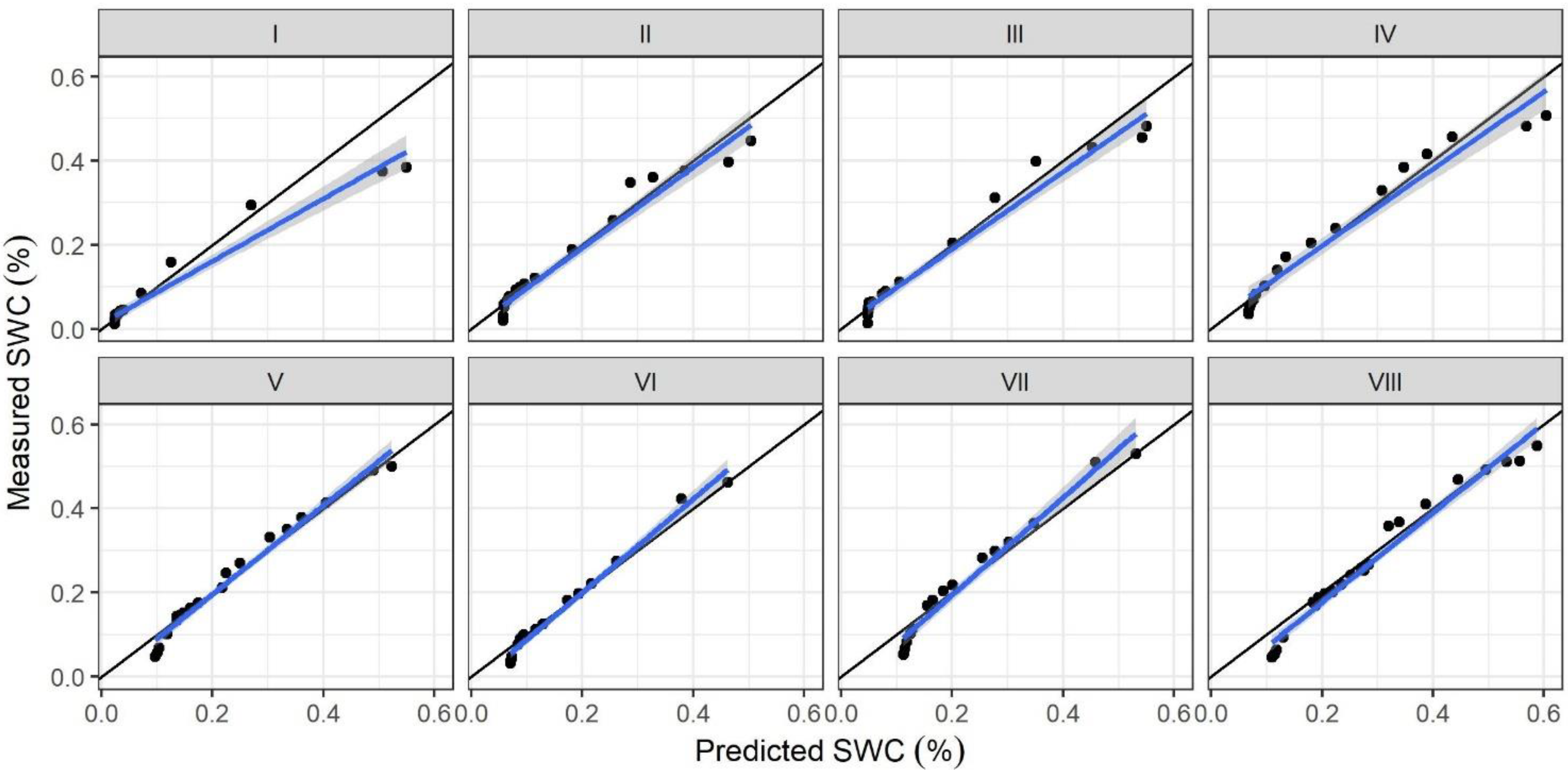
3.2. Model Performance if Only 5 Measurements between −60 and −15,000 cm Were Used in the MH-MCMC Approach and the RETC Program
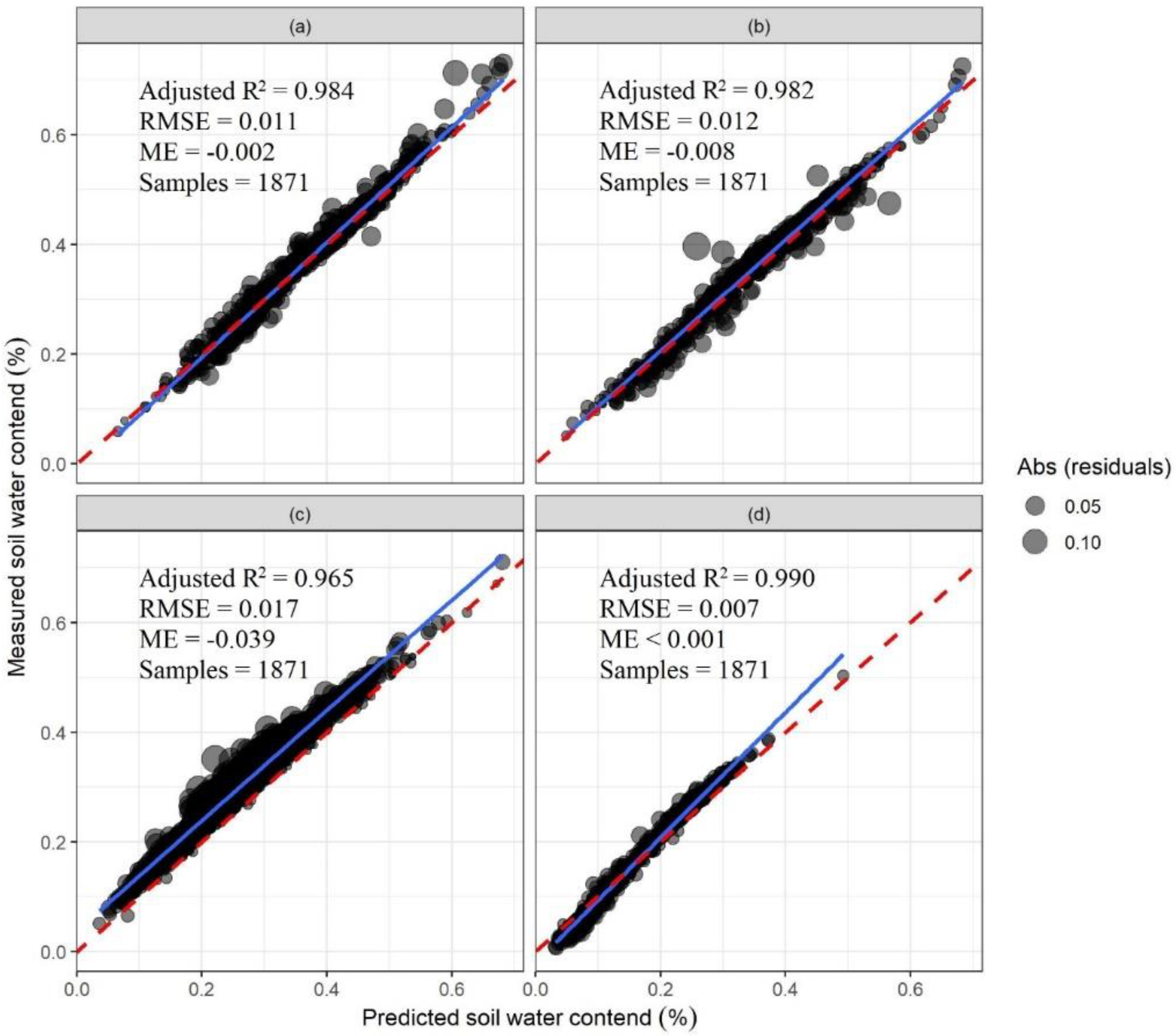
3.3. Model Performance over All 1871 Soils in the NCSS Dataset
4. Discussion
5. Conclusions
Author Contributions
Funding
Informed Consent Statement
Data Availability Statement
Acknowledgments
Conflicts of Interest
Appendix A

| Soil | Texture | Suction Matric (cm) | Volumetric Soil Water Content |
|---|---|---|---|
| I | Sand | −60 | 0.0446 |
| −102 | 0.0304 | ||
| −142.9 | 0.0336 | ||
| −403.1 | 0.0208 | ||
| −15,306 | 0.0112 | ||
| II | Sandy loam | −51 | 0.2580 |
| −102 | 0.1889 | ||
| −295.9 | 0.1213 | ||
| −510.2 | 0.1072 | ||
| −15,101.9 | 0.0536 | ||
| III | Loam | −61.2 | 0.4316 |
| −102 | 0.3978 | ||
| −214.3 | 0.2041 | ||
| −510.2 | 0.1105 | ||
| −15,306 | 0.0442 | ||
| IV | Silt loam | −71.4 | 0.4569 |
| −102 | 0.4154 | ||
| −204.1 | 0.3283 | ||
| −510.2 | 0.2365 | ||
| −15,306 | 0.1018 | ||
| V | Silt clay loam | −61.2 | 0.4141 |
| −102 | 0.3780 | ||
| −214.3 | 0.3315 | ||
| −510.2 | 0.2696 | ||
| −15,306 | 0.1342 | ||
| VI | Silt loam | −51 | 0.4615 |
| −102 | 0.4229 | ||
| −295.9 | 0.2753 | ||
| −510.2 | 0.2208 | ||
| −15,101.9 | 0.0998 | ||
| VII | Silt clay loam | −51 | 0.5306 |
| −102 | 0.5095 | ||
| −295.9 | 0.3643 | ||
| −510.2 | 0.3208 | ||
| −15,101.9 | 0.1690 | ||
| VIII | Silt loam | −50 | 0.4920 |
| −95.2 | 0.4680 | ||
| −203.9 | 0.4104 | ||
| −407.9 | 0.3672 | ||
| −15,116.4 | 0.1764 |
| MH-MCMC Approach | RETC Program | |||||||
|---|---|---|---|---|---|---|---|---|
| Soil | θr | θS | α | n | θr | θS | α | n |
| All measurements were used to obtain VG model parameters | ||||||||
| I | 0.0196 | 0.3870 | 0.0432 | 3.7672 | 0.0206 | 0.3850 | 0.0422 | 3.9701 |
| II | 0.0330 | 0.4532 | 0.0426 | 1.5655 | 0.0339 | 0.4489 | 0.0391 | 1.5755 |
| III | 0.0401 | 0.4770 | 0.0084 | 2.2000 | 0.0418 | 0.4748 | 0.0079 | 2.2908 |
| IV | 0.0323 | 0.5216 | 0.0170 | 1.3622 | 0.0369 | 0.5141 | 0.0132 | 1.3842 |
| V | 0.0255 | 0.5443 | 0.0461 | 1.2501 | 0.0000 * | 0.5378 | 0.0443 | 1.2197 |
| VI | 0.0333 | 0.6269 | 0.0324 | 1.4044 | 0.0377 | 0.5671 | 0.0185 | 1.4390 |
| VII | 0.0300 | 0.6719 | 0.0362 | 1.2676 | 0.0119 | 0.7238 | 0.0552 | 1.2370 |
| VIII | 0.0213 | 0.5500 | 0.0159 | 1.2521 | 0.0000 * | 0.5456 | 0.0144 | 1.2305 |
| Only 5 measurements at −60, −100, −200, −500, −15,000 cm matric potential were used to obtain VG model parameters | ||||||||
| I | 0.0235 | 0.5527 | 0.0587 | 3.7686 | 0.0101 | 0.4520 | 1.2765 | 1.5937 |
| II | 0.0569 | 0.5258 | 0.0591 | 1.7282 | 0.0461 | 0.8492 | 0.1995 | 1.5714 |
| III | 0.0475 | 0.5538 | 0.0120 | 2.1971 | 0.0528 | 0.4632 | 0.0071 | 2.7770 |
| IV | 0.0641 | 0.6305 | 0.0278 | 1.4721 | 0.0734 | 0.5900 | 0.0173 | 1.5191 |
| V | 0.0835 | 0.5568 | 0.0429 | 1.3388 | 0.0481 | 0.4980 | 0.0233 | 1.2816 |
| VI | 0.0673 | 0.5917 | 0.0237 | 1.5001 | 0.0948 | 0.4855 | 0.0067 | 1.9176 |
| VII | 0.1047 | 0.6420 | 0.0227 | 1.4061 | 0.1593 | 0.5564 | 0.0061 | 1.7973 |
| VIII | 0.0770 | 0.6189 | 0.0431 | 1.2510 | 0.0506 | 0.5308 | 0.0111 | 1.2615 |


References
- Schelle, H.; Heise, L.; Jänicke, K.; Durner, W. Water Retention Characteristics of Soils over the Whole Moisture Range: A Comparison of Laboratory Methods. Eur. J. Soil Sci. 2013, 64, 814–821. [Google Scholar] [CrossRef]
- Menezes, A.S.; Alencar, T.L.; Júnior, R.N.A.; Toma, R.S.; Romero, R.E.; Costa, M.C.G.; Cooper, M.; Mota, J.C.A. Functionality of the Porous Network of Bt Horizons of Soils with and without Cohesive Character. Geoderma 2018, 313, 290–297. [Google Scholar] [CrossRef]
- Richards, L.A.; Fireman, M. Pressure-Plate Apparatus for Measuring Moisture Sorption and Transmission by Soils. Soil Sci. 1943, 56, 395–404. [Google Scholar] [CrossRef]
- Schindler, U.; Durner, W.; von Unold, G.; Mueller, L.; Wieland, R. The Evaporation Method: Extending the Measurement Range of Soil Hydraulic Properties Using the Air-Entry Pressure of the Ceramic Cup. J. Plant Nutr. Soil Sci. 2010, 173, 563–572. [Google Scholar] [CrossRef]
- Campbell, G.S.; Smith, D.M.; Teare, B.L. Application of a Dew Point Method to Obtain the Soil Water Characteristic. In Experimental Unsaturated Soil Mechanics; Springer: Berlin/Heidelberg, Germany, 2007; pp. 71–77. [Google Scholar]
- Brooks, R.H.; Corey, A.T. Hydraulic Properties of Porous Media; Colorado State University: Fort Collins, CO, USA, 1964; pp. 1–34. [Google Scholar]
- Van Genuchten, M.T. A Closed-Form Equation for Predicting the Hydraulic Conductivity of Unsaturated Soils. Soil Sci. Soc. Am. J. 1980, 44, 892–898. [Google Scholar] [CrossRef] [Green Version]
- Fayer, M.J.; Simmons, C.S. Modified Soil Water Retention Functions for All Matric Suctions. Water Resour. Res. 1995, 31, 1233–1238. [Google Scholar] [CrossRef]
- Webb, S.W. A Simple Extension of Two-Phase Characteristic Curves to Include the Dry Region. Water Resour. Res. 2000, 36, 1425–1430. [Google Scholar] [CrossRef]
- Khlosi, M.; Cornelis, W.M.; Douaik, A.; van Genuchten, M.T.; Gabriels, D. Performance Evaluation of Models That Describe the Soil Water Retention Curve between Saturation and Oven Dryness. Vadose Zone J. 2008, 7, 87–96. [Google Scholar] [CrossRef]
- Fredlund, D.G.; Xing, A. Equations for the Soil-Water Characteristic Curve. Can. Geotech. J. 1994, 31, 521–532. [Google Scholar] [CrossRef]
- Groenevelt, P.H.; Grant, C.D. A New Model for the Soil-Water Retention Curve That Solves the Problem of Residual Water Contents. Eur. J. Soil Sci. 2004, 55, 479–485. [Google Scholar] [CrossRef]
- Van Genuchten, M.T.; Leij, F.J.; Yates, S.R. The RETC Code for Quantifying the Hydraulic Functions of Unsaturated Soils; U.S. Department of Agriculture, Agricultural Research Service: Riverside, CA, USA, 1991; ISBN 9781848212664. [Google Scholar]
- Shi, W.; Li, Q.; Han, Q.; Wang, T.; Chen, X.; Zhang, Y. Performance Analysis of Soil Water Retention Curve Models Based on Different Fitting Optimization Algorithms. J. Water Res. Water Eng. 2020, 31, 157–165. [Google Scholar] [CrossRef]
- Shi, X.; Xu, S.; Liao, K. AM-MCMC Approach to Estimate van Genuchten Model Parameters. Soils 2012, 44, 345–350. [Google Scholar]
- Wang, L.; Huang, C.; Huang, L. Parameter Estimation of the Soil Water Retention Curve Model with Jaya Algorithm. Comput. Electron. Agric. 2018, 151, 349–353. [Google Scholar] [CrossRef]
- Zhang, J.; Wang, Z.; Luo, X. Parameter Estimation for Soil Water Retention Curve Using the Salp Swarm Algorithm. Water 2018, 10, 815. [Google Scholar] [CrossRef] [Green Version]
- Gabrié, M.; Rotskoff, G.M.; Vanden-Eijnden, E. Efficient Bayesian Sampling Using Normalizing Flows to Assist Markov Chain Monte Carlo Methods. arXiv 2021, arXiv:2107.08001. [Google Scholar]
- Gao, H.; Zhang, J.; Liu, C.; Man, J.; Chen, C.; Wu, L.; Zeng, L. Efficient Bayesian Inverse Modeling of Water Infiltration in Layered Soils. Vadose Zone J. 2019, 18, 1–13. [Google Scholar] [CrossRef] [Green Version]
- Zhang, J.; Li, W.; Zeng, L.; Wu, L. An Adaptive Gaussian Process-Based Method for Efficient Bayesian Experimental Design in Groundwater Contaminant Source Identification Problems. Water Resour. Res. 2016, 52, 5971–5984. [Google Scholar] [CrossRef] [Green Version]
- Carsel, R.F.; Parrish, R.S.; Jones, R.L.; Hanse, J.L.; Lamb, R.L. Characterizing the Uncertainty of Pesticide Leaching in Agricultural Soils. J. Contam. Hydrol. 1988, 2, 111–124. [Google Scholar] [CrossRef]
- Duan, Q.; Gupta, V. SAC-SMA. Water Resour. Res. 1992, 28, 1015–1031. [Google Scholar] [CrossRef]
- Vrugt, J.A.; Gupta, H.V.; Bouten, W.; Sorooshian, S. A Shuffled Complex Evolution Metropolis Algorithm for Optimization and Uncertainty Assessment of Hydrologic Model Parameters. Water Resour. Res. 2003, 39, 1–14. [Google Scholar] [CrossRef] [Green Version]
- Lu, S.; Ren, T.; Lu, Y.; Meng, P.; Sun, S. Extrapolative Capability of Two Models That Estimating Soil Water Retention Curve between Saturation and Oven Dryness. PLoS ONE 2014, 9, e113518. [Google Scholar] [CrossRef]
- Lu, S.; Ren, T.; Gong, Y.; Horton, R. Evaluation of Three Models That Describe Soil Water Retention Curves from Saturation to Oven Dryness. Soil Sci. Soc. Am. J. 2008, 72, 1542–1546. [Google Scholar] [CrossRef]
- Schaap, M.G.; Leij, F.J.; Van Genuchten, M.T. Rosetta: A Computer Program for Estimating Soil Hydraulic Parameters with Hierarchical Pedotransfer Functions. J. Hydrol. 2001, 251, 163–176. [Google Scholar] [CrossRef]
- Haario, H.; Saksman, E.; Tamminen, J. An Adaptive Metropolis Algorithm. Bernoulli 2001, 7, 223–242. [Google Scholar] [CrossRef] [Green Version]
- Geyer, C.J. Practical Markov Chain Monte Carlo. Stat. Sci. 1992, 7, 473–483. [Google Scholar] [CrossRef]
- Wang, H.; Wang, C.; Wang, Y.; Gao, X.; Yu, C. Bayesian Forecasting and Uncertainty Quantifying of Stream Flows Using Metropolis–Hastings Markov Chain Monte Carlo Algorithm. J. Hydrol. 2017, 549, 476–483. [Google Scholar] [CrossRef] [Green Version]
- Smith, A.F.M.; Roberts, G.O. Bayesian Computation Via the Gibbs Sampler and Related Markov Chain Monte Carlo Methods. J. R. Stat. Soc. Ser. B 1993, 55, 3–23. [Google Scholar] [CrossRef]
- R Core Team. R: A Language and Environment for Statistical Computing; R Foundation for Statistical Computing: Vienna, Austria, 2019. [Google Scholar]
- Rotunno Filho, O.C.; de Araujo, A.A.M.; Xavier, L.N.R.; Moreira, D.M.; Di Bello, R.C.; Xavier, A.E.; de Araujo, L.M.N. Soil Moisture and Soil Water Storage Using Hydrological Modeling and Remote Sensing; Hartemink, A.E., McBratney, A.B., Eds.; Springer: Cham, Switzerland, 2014; ISBN 9783319060125. [Google Scholar]
- Lilly, A.; Lin, H. Using Soil Morphological Attributes and Soil Structure in Pedotransfer Functions. Dev. soil Sci. 2004, 30, 115–141. [Google Scholar] [CrossRef]
- Jian, J.; Shiklomanov, A.; Shuster, W.D.; Stewart, R.D. Predicting Near-Saturated Hydraulic Conductivity in Urban Soils. J. Hydrol. 2021, 595, 126051. [Google Scholar] [CrossRef]
- Martino, L.; Casarin, R.; Leisen, F.; Luengo, D. Adaptive Independent Sticky MCMC Algorithms. EURASIP J. Adv. Signal Process. 2018, 2018, 5. [Google Scholar] [CrossRef] [Green Version]
- Chen, Y.; Dwivedi, R.; Wainwright, M.J.; Yu, B. Fast MCMC Sampling Algorithms on Polytopes. J. Mach. Learn. Res. 2018, 19, 2146–2231. [Google Scholar]
- Hassibi, B.; Hansen, M.; Dimakis, A.G.; Alshamary, H.A.J.; Xu, W. Optimized Markov Chain Monte Carlo for Signal Detection in MIMO Systems: An Analysis of the Stationary Distribution and Mixing Time. IEEE Trans. Signal Process. 2014, 62, 4436–4450. [Google Scholar] [CrossRef] [Green Version]


| Parameters | Prior | Note |
|---|---|---|
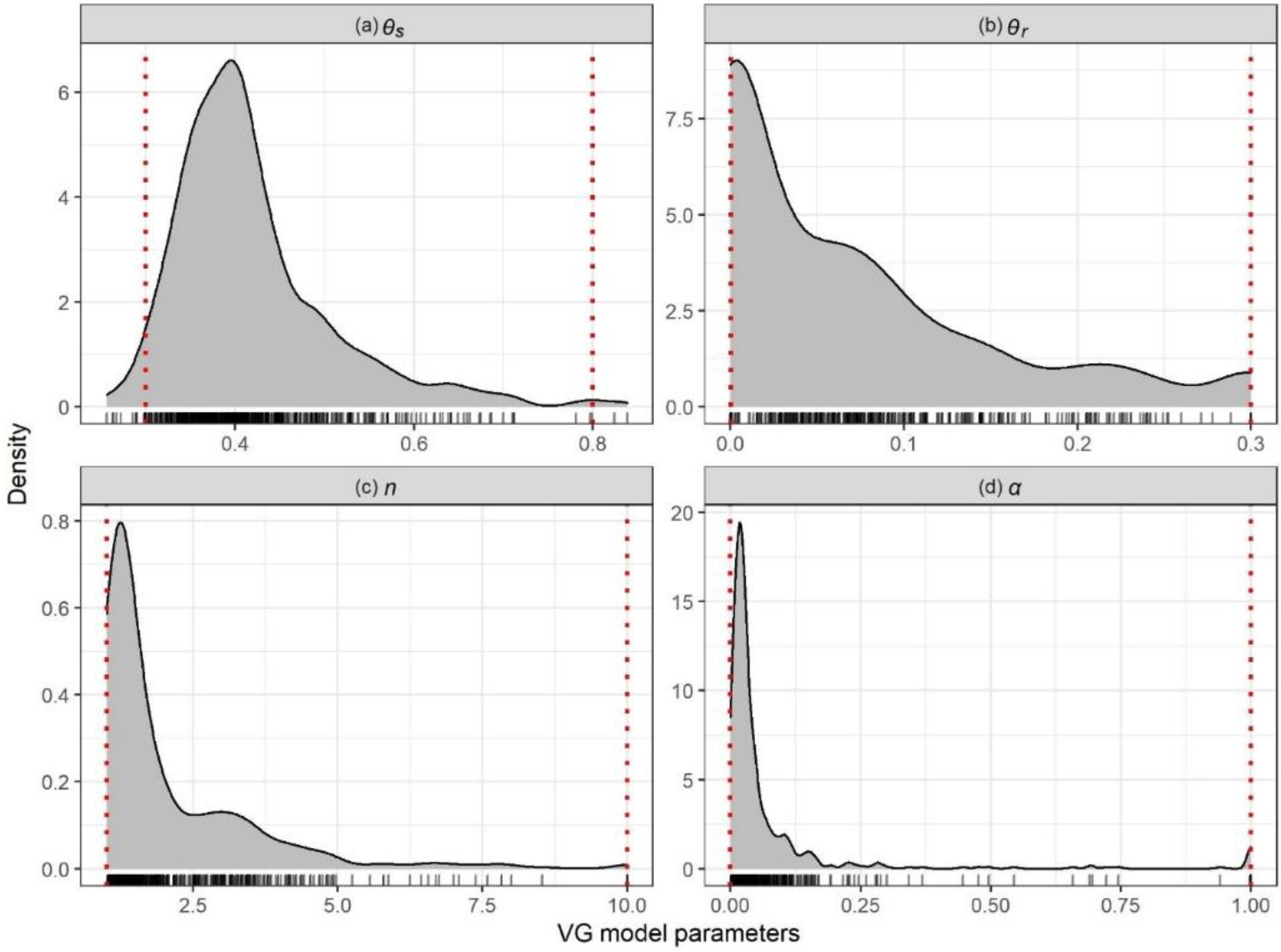
| 0.30–0.80 | Adjusted based on UNSODA (Figure 2) and ref. [15] | |
| 0.0003–0.30 | Adjusted based on UNSODA (Figure 2) and ref. [15] | |
| 0.0001–1.0 | Adjusted based on UNSODA (Figure 2) and ref. [15] | |
| n | 1.0–10 | Adjusted based on UNSODA (Figure 2) and ref. [15] |
| Soil | Adjusted R2 | RMSE | ME | Adjusted R2 | RMSE | ME | Samples |
|---|---|---|---|---|---|---|---|
| All SWC Measurements Were Used to Parameterize the VG Model | |||||||
| MCMC | RETC | ||||||
| I (Sand) | 0.997 | 0.006 | <0.0001 | 0.998 | 0.006 | 0.0007 | 19 |
| II (Sandy loam) | 0.985 | 0.018 | −0.002 | 0.985 | 0.018 | <0.0001 | 19 |
| III (Loam) | 0.991 | 0.016 | −0.001 | 0.991 | 0.016 | <0.0001 | 19 |
| IV (Silt loam) | 0.993 | 0.013 | −0.005 | 0.995 | 0.012 | <0.0001 | 17 |
| V (Silt clay loam) | 0.995 | 0.010 | −0.003 | 0.996 | 0.009 | 0.0002 | 19 |
| VI (Silt loam) | 0.991 | 0.013 | −0.005 | 0.992 | 0.012 | <0.0001 | 15 |
| VII (Silt clay loam) | 0.992 | 0.013 | −0.006 | 0.993 | 0.013 | <0.0001 | 16 |
| VIII (Silt loam) | 0.991 | 0.015 | −0.003 | 0.993 | 0.013 | 0.0001 | 24 |
| Only 5 SWC measurements were used to parameterize the VG model (but all data were used for model performance evaluation) | |||||||
| MCMC | RETC | ||||||
| I (Sand) | 0.950 | 0.027 | 0.013 | 0.872 | 0.044 | −0.0454 | 19 |
| II (Sandy loam) | 0.956 | 0.031 | 0.006 | 0.900 | 0.046 | 0.0182 | 19 |
| III (Loam) | 0.970 | 0.029 | 0.007 | 0.988 | 0.018 | 0.0026 | 19 |
| IV (Silt loam) | 0.952 | 0.037 | 0.005 | 0.972 | 0.028 | 0.0129 | 17 |
| V (Silt clay loam) | 0.978 | 0.021 | 0.002 | 0.994 | 0.011 | 0.0032 | 19 |
| VI (Silt loam) | 0.985 | 0.017 | 0.004 | 0.963 | 0.026 | 0.0141 | 15 |
| VII (Silt clay loam) | 0.968 | 0.027 | 0.002 | 0.911 | 0.045 | 0.0246 | 16 |
| VIII (Silt loam) | 0.971 | 0.027 | 0.018 | 0.993 | 0.014 | 0.0136 | 24 |
Publisher’s Note: MDPI stays neutral with regard to jurisdictional claims in published maps and institutional affiliations. |
© 2022 by the authors. Licensee MDPI, Basel, Switzerland. This article is an open access article distributed under the terms and conditions of the Creative Commons Attribution (CC BY) license (https://creativecommons.org/licenses/by/4.0/).
Share and Cite
Du, X.; Du, C.; Radolinski, J.; Wang, Q.; Jian, J. Metropolis-Hastings Markov Chain Monte Carlo Approach to Simulate van Genuchten Model Parameters for Soil Water Retention Curve. Water 2022, 14, 1968. https://0-doi-org.brum.beds.ac.uk/10.3390/w14121968
Du X, Du C, Radolinski J, Wang Q, Jian J. Metropolis-Hastings Markov Chain Monte Carlo Approach to Simulate van Genuchten Model Parameters for Soil Water Retention Curve. Water. 2022; 14(12):1968. https://0-doi-org.brum.beds.ac.uk/10.3390/w14121968
Chicago/Turabian StyleDu, Xuan, Can Du, Jesse Radolinski, Qianfeng Wang, and Jinshi Jian. 2022. "Metropolis-Hastings Markov Chain Monte Carlo Approach to Simulate van Genuchten Model Parameters for Soil Water Retention Curve" Water 14, no. 12: 1968. https://0-doi-org.brum.beds.ac.uk/10.3390/w14121968