Article

Diagnosing Atmospheric Influences on the Interannual 18O/16O Variations in Western U.S. Precipitation

1
Department of Earth Sciences, University of Southern California, Zumberge Hall of Science (ZHS), 3651 Trousdale Pkwy, Los Angeles, CA 90089, USA
2
Atmosphere and Ocean Research Institute, University of Tokyo, General Research Building 211a, 5-1-5 Kashiwanoba, Kashiwa Chiba 277-8568, Japan
*
Author to whom correspondence should be addressed.
Submission received: 28 April 2013 / Revised: 6 June 2013 / Accepted: 9 July 2013 / Published: 25 July 2013
(This article belongs to the Special Issue Environmental Tracers)

Abstract

:
Many climate proxies in geological archives are dependent on the isotopic content of precipitation (δ18Op), which over sub-annual timescales has been linked to temperature, condensation height, atmospheric circulation, and post-condensation exchanges in the western U.S. However, many proxies do not resolve temporal changes finer than interannual-scales. This study explores causes of the interannual variations in δ18Op within the western U.S. Simulations with the Isotope-incorporated Global Spectral Model (IsoGSM) revealed an amplifying influence of post-condensation exchanges (i.e., raindrop evaporation and vapor equilibration) on interannual δ18Op variations throughout the western U.S. Mid-latitude and subtropical vapor tagging simulations showed that the influence of moisture advection on δ18Op was relatively strong in the Pacific Northwest, but weak over the rest of the western U.S. The vapor tags correlated well with interannual variations in the 18O/16O composition of vapor, an indication that isotopes in vapor trace atmospheric circulation. However, vertical-tagging simulations revealed a strong influence of condensation height on δ18Op in California. In the interior of the western U.S., a strong temperature effect was found only after annual mean temperatures were weighted by monthly precipitation totals. These multiple influences on δ18Op complicate interpretations of western U.S. climate proxies that are derived from isotopes in precipitation.

1. Introduction

Stable oxygen and hydrogen isotopes (primarily 18O and deuterium) preserved in geological archives are commonly used as proxies of past climatic changes (e.g., see reviews: [1,2,3,4]). Many of these proxies are derived from meteoric waters and thus record temporal variations in the isotopic composition of precipitation (hereafter δ18Op, where the isotopic composition is defined as: δ = R/RSTANDARD 1, where R is the heavy to light isotope ratio). It is important for the interpretation of climate proxies to better understand the causes of temporal variations in δ18Op within a given region. Within the tropics and subtropics, δ18Op is typically linked to changes in precipitation rates (the amount effect) [5,6,7,8,9,10,11,12], whereas measurements from outside of the tropics and subtropics usually show correlations between δ18Op and air temperature (the temperature effect) [5,13,14,15,16]. However, within many middle latitude regions the relationship between δ18Op and climatic variables is not always as clear, which creates difficulties when interpreting climate proxies within these latitudes. It is likely that the isotopic composition of precipitation that falls in the middle latitudes is subject to a combination of influences. This study focuses on the western U.S., with the intent to understand the primary influences on the year-to-year changes in δ18Op.
Previous studies of the western U.S. have examined δ values from ice cores [17,18], tree cellulose [16,19,20], speleothems [21,22,23], leaf wax n-alkanes [24], and lacustrine sediment archives [25,26,27,28]. These records provide estimates of δ18Op variations on several timescales, including seasonal, interannual and interdecadal. The variations within each record have been attributed to changes in near surface air-temperature, precipitation amount, surface latent heat release, and/or storm trajectories.
On sub-hourly timescales, precipitation δ variations have been linked to changes in condensation height [29] and raindrop re-evaporation [30]. At weekly to seasonal timescales, studies have suggested that seasonal temperature variations strongly impact δ18Op in the western U.S. [31,32], while several other studies [33,34,35,36] have suggested that storm trajectories were the primary influence on precipitation δ values. Recently, Buenning et al. [37] found through model sensitivity experiments and tagging simulations that the seasonal cycle of δ18Op was primarily a result of seasonal changes in vapor condensation height along the west coast of the U.S. However, one of the remaining issues of Buenning et al. [37] was whether or not the same mechanism drives interannual variations in precipitation δ values within the region, which would likely be more valuable for the interpretation of paleoclimate archives.
This study aims to answer the question of which mechanism(s) primarily drive interannual δ18Op variations in the western U.S. by using model simulations. The following sections discuss the model, the model experiments (Section 2), and validation (Section 3). Sensitivity experiments are assessed to find which fractionation process has the largest influence on interannual δ18Op variations within the model, and the influences of post-condensation exchanges, condensation height, moisture advection, and temperature on interannual δ18Op variations are discussed and quantified (Section 4). Finally, the paper concludes with a summary of the results and a discussion of the implications of the findings (Section 5).

2. Methods

A methodology similar to Buenning et al. [37] is used here to diagnose the cause of the interannual variations in δ18Op. The model used for this study is the Experimental Climate Prediction Center’s (ECPC) Isotope-incorporated Global Spectral Model (IsoGSM) [38]. The atmosphere in IsoGSM has 28 vertical layers, and the chosen horizontal resolution of the model is given by triangular truncation of the spherical harmonic spectrum at wave number 62 (approximately 1.85° longitude by 1.85° latitude). The model is forced with prescribed sea surface temperatures and sea-ice conditions from the optimal interpolation weekly data set, downloaded from the ECPC database [39]. Each IsoGSM simulation runs from 1953 through 2010 with a 10-minute time-step, and each simulation is spectrally nudged to the same wind and temperature fields (The National Centers for Environmental Predictions and National Center for Atmospheric Research Reanalysis version 1 [40]) every six hours. Yoshimura and Kanamitsu [41] describe the specific details of the spectral nudging technique.
IsoGSM accounts for water isotopologues (H2O, H218O, and HDO) in all three phases within the simulated atmosphere, and fractionation factors (defined as α = Rcd = Rg, where subscripts cd and g refer to condensed phase and gas, respectively) are computed and applied when phase changes occur. Using the temperature-dependent formulations of Majoube et al. [42,43], equilibrium oxygen isotopic fractionation is applied during vapor condensation in the atmosphere (αeqcon) and during both ocean (αeqev) and raindrop (αeqrev) evaporation. Kinetic fractionation is also accounted for in IsoGSM during ocean evaporation (αkev) [44] and vapor deposition onto ice crystals (αkcon) [45]. Isotopic exchange and both equilibrium and kinetic fractionation during raindrop evaporation is estimated following Stewart [46]. It is assumed that 45% of falling raindrops equilibrate with surrounding vapor for convective precipitation and 95% equilibrates for stratiform precipitation.
Interannual δ18Op variability is first evaluated in an unperturbed control simulation (CTRL). The model is then used to determine which fractionation processes contribute to the interannual δ18Op variations. Sensitivity experiments were conducted with IsoGSM by “turning off” isotope fractionation. Note, these model experiments were conducted previously by Buenning et al. [37]. Each sensitivity experiment (name in all capitals) turned off individual fractionation processes by setting the isotopic fractionation factors (α variables defined above) equal to one (a list and description of each experiment is given in Table 1). Two of the model experiments assess the influence of equilibrium oxygen isotope fractionation processes [42,43] on interannual δ18Op variance. These processes are equilibrium oxygen isotope fractionation during ocean evaporation (αeqev, NOFEQ1) and condensation in the atmosphere (αeqcon, NOFEQ2). These two experiments removed both the temperature dependence of αeq and the isotope effect (i.e., preferential evaporation or rainout). As such, two additional simulations were conducted where only the temperature dependence is removed by setting the equilibration temperature to a constant value, globally (CONFEQ1 and CONFEQ2, with αeqev = 1.00980653 and αeqcon = 1.01162795, respectively). Simulations that removed kinetic oxygen isotope fractionation were performed, which included isotope fractionation during ocean evaporation (αkev, NOFKI1) [44] and vapor deposition onto ice crystals (αkcon, NOFKI2) [45]. The final fractionation experiment was performed where raindrop equilibration rates were set equal to zero. This experiment removes all isotope effects associated with post-condensation exchanges, including vapor-rain equilibration and both equilibrium and kinetic fractionation during raindrop evaporation (NORNEV) [11,30,46,47,48] (see Yoshimura et al. [30] for equations used in IsoGSM’s rain exchange model).
Table 1. Name and description of Isotope-incorporated Global Spectral Model (IsoGSM) simulations.
Simulation nameDescription
CTRLUnperturbed control simulation
NOFEQ1Equilibrium oxygen isotopic fractionation during ocean water evaporation is turned off (αeqev = 1)
NOFEQ2Equilibrium oxygen isotopic fractionation during condensation is turned off (αeqcon = 1)
NORNEVAll oxygen isotopic fractionation associated with raindrop evaporation is turned off
CONFEQ1Equilibrium oxygen isotopic fractionation during ocean water evaporation is set to constant, removing the temperature dependence (αeqev = 1.00980653, T = 293 K)
CONFEQ2Equilibrium oxygen isotopic fractionation during condensation is set to a constant, removing the temperature dependence (αeqcon = 1.01162795, T = 274 K)
NOFKI1Kinetic oxygen isotopic fractionation during ocean water evaporation is turned off (αkev = 1)
NOFKI2Kinetic oxygen isotopic fractionation during vapor deposition onto ice is turned off (αkcon = 1)
TAGYTagging simulation where tag1 is applied within 20°–40° N and 140°–170° W; Tag 2 is applied within 40°–60° N and 140°–170° W.
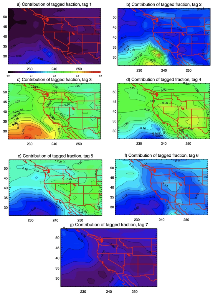
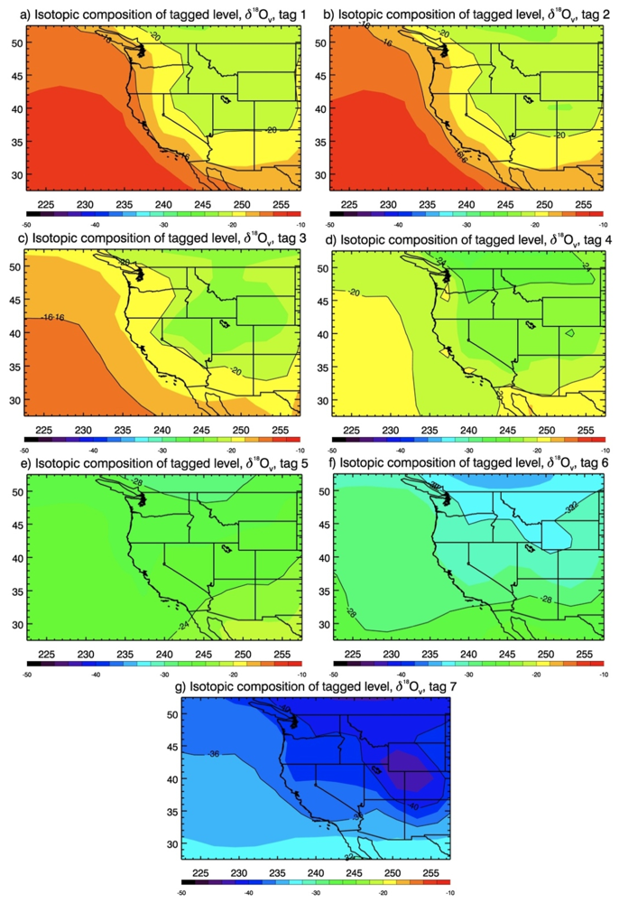
TAGZTagging simulation where 14 separate tags are applied to the 28 vertical σ layers (2 layers per tag). Tag 1 is applied to the surface layer and layer 2; tag 2 is applied to layers 3 and 4; tag 3 is applied to layers 5 and 6; and so on to up to layers 27 and 28. This simulation is actually a combination of 7 simulations, with each model run simulating two of the tags.
Vertical tagging simulations were performed with IsoGSM, such that tagged vapor mixing ratios were set equal to “normal” vapor mixing ratios at specific levels (TAGZ). Unlike the TAGLEV simulation of Buenning et al. [37] (which only tagged two layers), 14 individual tags were assigned to the 28 individual layers in IsoGSM to account for condensation height (one tag per 2 atmospheric levels). Tags were removed from the atmosphere if the tagged vapor advects vertical tagging level. Thus, resulting precipitation of each vertical water tag will quantify the amount of total precipitation from 14 different vertical levels of the atmosphere.
To account for interannual variations in moisture advection, a horizontal tagging simulation was performed with IsoGSM (similar to the TAGLAT simulation of Buenning et al. [37]), where subtropical moisture was tagged within 20°–40° N and 140°–170° W and middle latitude vapor was tagged within 40°–60° N and 140°–170° W (TAGY). For the TAGY simulation, tagged vapor mixing ratios were set to “normal” vapor mixing ratios within each of the two tagging regions at every model time-step. When vapor from one tagging region is transported by the winds into the other region, it is immediately removed to avoid vapor having both tags. Outside of the tagging regions, the tagged vapor is treated the same as normal vapor, except they are not used in the energy calculations (i.e., the vapor tags are allowed to advect, mix, condense, and rainout). It is important to note that the tracer method used here differs with the typical method of tagging vapor that evaporates off the ocean surface. The method used here allows a direct quantification of the amount of precipitation and vapor that was advected from each tagging region. Because both the TAGY and the CTRL simulations are nudged to the same reanalysis wind fields, δ18O values can be compared to the fraction of vapor and precipitation with each tag. Correlation coefficients were calculated at each grid cell in the western U.S., to quantify the co-variability between δ18O values and tagged fraction (for both TAGY and TAGZ).

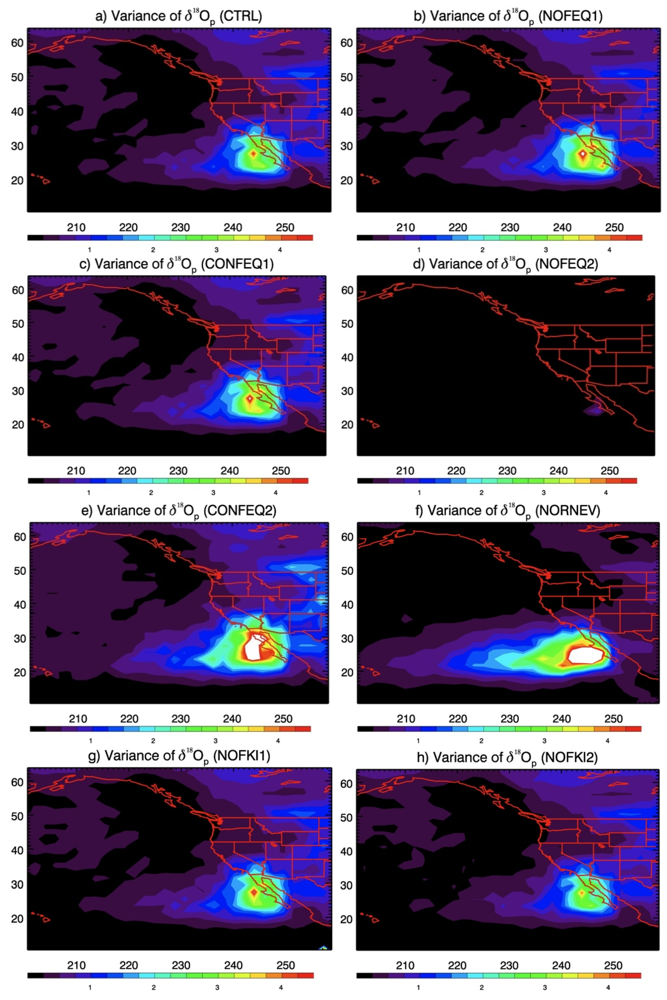
3. Simulated δ18Op Variability

Previous studies have validated IsoGSM’s ability to capture temporal variations on several timescales. Yoshimura et al. [38] first compared IsoGSM results with measurements from the Global Network for Isotopes in Precipitation (GNIP). By comparing IsoGSM and other models against long records (>45 years) from GNIP stations, they concluded that an accurate simulation of atmospheric winds is necessary to reliably model interannual δ18Op variations. These results showed how spectral nudging constrains the simulated wind and temperature fields, which in turn allows for good model-data agreement. Within central/coastal California, Yoshimura et al. [30] demonstrated the ability of the regional version of IsoGSM (IsoRSM) to capture sub-hourly isotopic variations. Berkelhammer et al. [36] further validated IsoGSM on weekly timescales at 6 sites in California over the span of 2000–2005. Buenning et al. [37] showed how IsoGSM was able to capture the seasonal wintertime drop in δ18Op at 16 different sites in British Columbia, Washington, Oregon, and California. However, the lack of long continuous records of δ18Op in regions outside of Europe [12] makes it difficult to validate the model on interannual to multi-decadal timescales, especially in the western U.S.
To address this issue, studies have used tree cellulose δ18O values (δ18Oc) as a measure of δ18Op variability [16,19,49,50,51]. This type of comparison typically involves the use of an offline biogeochemical model calculation that uses atmospheric model outputs to estimate δ18Oc. Berkelhammer and Stott [16] used IsoGSM output as input for a geochemical model put forth by Roden et al. [52] and found good model agreement with 2 bristlecone pine trees in the Rocky Mountains of Colorado. They note that the model’s ability to capture the interannual variations declines going back in time (especially prior to 1950), which was attributed to a decline in the quality of the reanalysis forcing data due to less observational constraints. The same type of decline in IsoGSM model/observation agreement was found in southern California by Kanner et al. [53], who found that the model performed exceptionally well for the 1979–2004 period, but found a decline in model agreement from 1953 to 1979. They noted that the discrepancy between the two time periods could be a result of the increased constraints on the reanalysis data after 1979 (i.e., the satellite era).

4. Attributing Interannual Isotopic Variations

Interannual variance is calculated at each grid cell by computing annual means (centered on the winter wet season: July through June) for the simulated period; a total of 56 annual means per grid cell (the first model year is not used). Figure 1a shows a map of the interannual variance of δ18Op for the control simulation (CTRL) over the Pacific and western North America. The largest variance occurs over the Baja Peninsula of Mexico, and the variance decreases northward along the coast and inland towards the Southwest U.S. This is consistent with the results of Buenning et al. [37], who showed that observed seasonal variations along the western U.S. coastline were largest for southern stations and decreased northward. Figure 1b–g shows the spatial distribution of interannual δ18Op variance for the seven model fractionation experiments. All but two of the experiments showed the same general pattern of variance as the control simulation; removing equilibrium oxygen isotopic fractionation during condensation (NOFEQ2) and removing post-condensation exchanges (NORNEV) being the two exceptions. These results show the importance of isotopic rainout and post-condensation exchanges in the western U.S., and suggest that other isotope processes (e.g., ocean evaporation, kinetic fractionation, and the temperature-dependence of αeq) have less influence on interannual δ18Op variability. The variance was almost completely removed when equilibrium fractionation during condensation was removed (NOFEQ2), as was the case for the seasonal δ18Op cycle [37]. The variance difference between the control simulation (CTRL) and the simulation that removed post-condensation exchanges (NORNEV) is discussed in more detail in the subsection below.

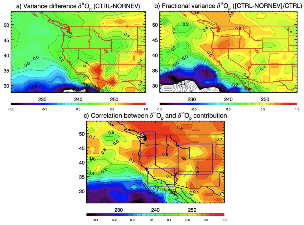
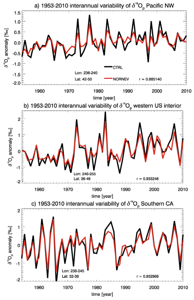
4.1. Post-Condensation Exchanges

Post-condensation exchanges were removed by setting raindrop equilibration rates equal to zero, which not only prevented rain from isotopically equilibrating with the surrounding vapor, but it also prevented raindrops from fractionating during evaporation [30]. The absolute change in the variance due to post-condensation exchanges can be quantified by taking the difference in δ18Op variance between the CTRL and NORNEV simulations (Figure 2a). In general, the NORNEV experiment caused δ18Op variance to decrease over land, but increase over the ocean southwest of the Baja Peninsula (Figure 2a). The fractional change to the variance due to post-condensation exchanges can be quantified by dividing the variance difference (values in Figure 2a) by the variance from the control simulation (values in Figure 1a), which is shown in Figure 2b. The fraction of the variance that is removed by the model experiment (NORNEV) is more uniform over land than the absolute change, with the highest fractional change occurring over Oregon (Figure 2b). In general post-condensation exchanges contribute about 60% to the total interannual δ18Op variance in the western U.S., reaching as high as 74% over central Oregon.
What is not apparent in Figure 2a,b is that the removal of post-condensation exchanges (NORNEV) dampened interannual variations that existed in the control simulation. Figure 3 shows regional average time series for the CTRL and NORNEV simulations for the Pacific Northwest, the western US interior, and southern/central California. The curves in Figure 3 show that the variations produced by both simulation are similar and the inclusion of post-condensation exchanges (in CTRL) amplify the maxima and minima that would have existed without the processes. To demonstrate that this is not unique to these three regions, the contribution of post-condensation exchanges to interannual δ18Op variations (defined as the control minus experiment) is correlated to each original time series from each grid cell from the control simulation (Figure 2c). These calculations produce high positive correlations over most of the western U.S., ranging from 0.6 to 0.9 (Figure 2c). The highest correlations were found where the influence of post-condensation exchanges was also high (e.g., over Oregon). These results reveal that post-condensation exchanges contribute about 60%–75% of the δ18Op variance (Figure 2b), mostly by amplifying year-to-year maxima and minima caused by other processes (Figure 2c and Figure 3).
Figure 1. (a) Spatial distribution of variance of δ18Op for the control simulation; and (b)–(h) 7 model experiments. Variance is calculated from interannual time series at each grid cell. Contour intervals are 0.25‰.
Water 05 01116 g001
Figure 2. (a) Variance difference between the control simulation (CTRL) simulation and the simulation that removed isotope effects from post-condensation exchanges (NORNEV); (b) The same variance difference divided by the variance of the CTRL simulation; (c) Correlation between interannual δ18Op variations from the CTRL simulation and the difference in δ18Op between the CTRL simulation and NORNEV simulation. Open purple rectangles in panel (c) show the boxed regions for Figure 3.
Water 05 01116 g002
Figure 3. Regional average interannual time series of δ18Op for the CTRL and NORNEV simulations. The panels display the (a) Pacific Northwest; (b) the interior of the western U.S.; (c) and central/southern California.
Water 05 01116 g003

4.2. Condensation Height

Buenning et al. [37] found that δ18Op seasonality along the western U.S. coast was primarily driven by seasonal changes to condensation height. To examine if condensation height is also influencing interannual δ18Op variations, vertical tagging simulations were performed with IsoGSM, such that the 28 atmosphere levels in IsoGSM were divided into 14 tagged-levels, and 14 separate tags were added to each of the 14 levels. The tagging was done such that tagged vapor was set equal to normal vapor within each level at every time step. Tagged vapor is allowed to advect and condense in the predefined tagged level; however, if the vapor is transported vertically across tagged level boundaries, it is immediately removed. This approach is similar to the TAGLEV simulation conducted by Buenning et al. [37], with the exception that the atmosphere is divided into 14 tagged-levels and not 2.
For most areas, the bottom 14 levels of IsoGSM (the bottom 7 tagged-levels) contributed over 95% of the total precipitation during the course of a typical year. As such, results from the bottom seven tags are presented here. Figure 4 shows the interannual correlation between the fraction of precipitation with a vertical tag (i.e., ptag/ptotal) and δ18Op for each of the 7 tags at each grid cell in the western U.S. Though the correlation coefficients do not imply causation, they do quantify the co-variability between δ18Op and condensation height. They will also reveal locations where there are connections between δ18Op and condensation height. For the bottom 3 tags (tags 1–3, hereafter) correlations are high and positive throughout most of California, with the largest correlation occurring along the coast of southern and central California (Figure 4a–c). Correlations for tags 1–3 are also high and positive in northern Oregon and southern Washington. The correlations become weaker for the inland western states and northeastern California.
Figure 4. (a)–(g) Correlation between interannual δ18Op variations and the fraction of precipitation from each of the vertical tags. Correlations with the bottommost tag is shown in panel (a) (tag 1); and correlations with higher level tags are shown in panels (b)–(g). Contour intervals are 0.1. Absolute values of r above 0.263 are significant above the 95% confidence level.
Water 05 01116 g004
The correlation changes significantly for tag 4 (Figure 4d) with many regions seeing reduced correlation, except for parts of southern California, where r-values are at their highest. High negative correlations exist between δ18Op and the fraction of precipitation with higher-level tags (hereafter, tags 5–7) for many regions in the western U.S. (Figure 4e–g). These shifts from positive to negative correlations suggests that annual mean δ18Op tends to be lower (higher) during years when a larger fraction of the precipitation was derived from higher (lower) in the atmosphere, where vapor δ18O values are typically more (less) negative. The spatial distributions of the correlation coefficients for the higher-level tags (5–7) are almost mirror images of the lower level tags (1–3), but of opposite sign (Figure 4). Like tags 1–3, correlations are high (though negative) for almost all of California, southern Washington, and northern Oregon. Also, correlations between δ18Op and the fraction of precipitation with tags 5–7 are significantly reduced for the inland western states. The correlations in Figure 4 reveal evidence of an influence of condensation height on interannual δ18Op variations in some, but not all, regions of the western U.S., similar to the isotope seasonality results of Buenning et al. [37].
To quantify the contribution of condensation height on interannual δ18Op variations, multiple correlation coefficients were calculated for each location, using the fraction of precipitation from each tag (ptag/ptotal) as the predictor and δ18Op as the dependent variable. Based on the fractional contribution from each tag (discussed below), only tags 2–6 are used for each calculation. Though this approach is not a direct measurement of the contribution from condensation height, the r2 value does give a measure of shared variance, which can be used as a first order estimate of the fraction of the variance attributable to condensation height. Figure 5a shows the multiple correlation coefficients, suggesting that condensation height contributes roughly 25%–40% to interannual δ18Op variance in central and southern California (r ranging from 0.5 to 0.63). In coastal northern California, Oregon, and Washington, the contribution is slightly less at about 10%–15% (r ranging from 0.3 to 0.4). The r-values in the interior states of the western U.S. are not viewed as a contribution to the interannual variance because of the sign of the single variable correlations in Figure 4 (which indicates another effect/process is overriding interannual variations in condensation height in these regions). Performing the same calculations with δ18Op values from the NORNEV simulation resulted in higher r-values (Figure 5b), which is not surprising since the simulation removed processes that have already been shown to highly influence interannual δ18Op variations. These results show that condensation height is most influential on interannual δ18Op variations in southern and central California with decreasing influence northward into coastal Washington.
To demonstrate why condensation height drives interannual δ18Op variations in some regions more than others, Figure 6 shows the mean fractional contribution of precipitated tag to the total precipitation (the mean value used in the correlation calculation) for tags 1 through 7. The contribution of the bottom tag was only 3%–4% of the total precipitation, but the contribution of tag 2 was higher and above 10% in most grid cells. Tags 3–5 contributed the highest fraction to the total precipitation throughout the western U.S., ranging from about 20%–40% for each tag. Further up in the modeled atmosphere, the fractional contribution decreases sharply for tags 6 and 7, which are similar to tags 2 and 1, respectively.
Figure 5. (a) Multiple correlation between tags 2–6 (ptag/ptotal) and δ18Op from the CTRL simulation; and (b) the NORNEV simulation.
Water 05 01116 g005
Figure 6. (ag) The contribution of each vertical tag to the total precipitation. Closed contour intervals are 0.01.
Water 05 01116 g006
Figure 7 shows the mean isotopic composition associated with each vertical tag by amount weighting (based on tagged vapor) the δ18O value of vapor (δ18Ov) from the control (CTRL) simulation. Though the mean δ18Ov values of tags 1 and 2 are roughly the same, δ18Ov decreases upward, as would be expected due to vertical isotope gradients in δ18Ov [54,55,56]. Figure 8 shows the difference in δ18O values between tags 3 and 5 (i.e., Figure 7e minus Figure 7c), which are two of three tags that contributed the most to the total precipitation. The difference in the isotopic composition of vapor between the two tags clearly shows the vertical gradient (at levels that contribute the most to total precipitation) is strongest along the coastline and decreases inland. This feature is partially responsible for the strength of the condensation height effect over most of Washington, Oregon, and California.
Figure 8 does not reconcile why the influence of condensation height is strongest in southern and central California and decreases northward along the coast. Figure 9 displays the interannual variance of the fraction of precipitation with tags 3 and 5. The spatial distribution of the variance is remarkably similar to Figure 1f (the variance of δ18Op from the NORNEV simulation), showing that the largest variability was near the Baja Peninsula with decreased variance northward along the coast and inland. Not surprisingly, Figure 9 reveals that the influence of condensation height on δ18Op was strongest in regions where variations in condensation height were also large.
Figure 7. (ag) The isotopic composition of vapor (δ18Ov) corresponding with each of the vertical tags. Mean values are calculated by weighting vertical δ18Ov from the CTRL simulation by the vertical distribution of the given tag. The bottommost tag is shown in panel a (tag 1), and higher level tags are shown in panels (b)–(g). Contour intervals are 1‰.
Water 05 01116 g007
Figure 8. Difference between the isotopic composition of vapor between vertical tags 3 and 5 (Figure 7e and Figure 7c). More negative values indicate a steeper veritcal gradient in δ18O values of vapor (δ18Ov). Closed contour intervals are 0.5‰.
Water 05 01116 g008
Figure 9. Interannual variance of fraction of precipitation from (a) vertical tag 3; and (b) vertical tag 5.
Water 05 01116 g009

4.3. Circulation Effects

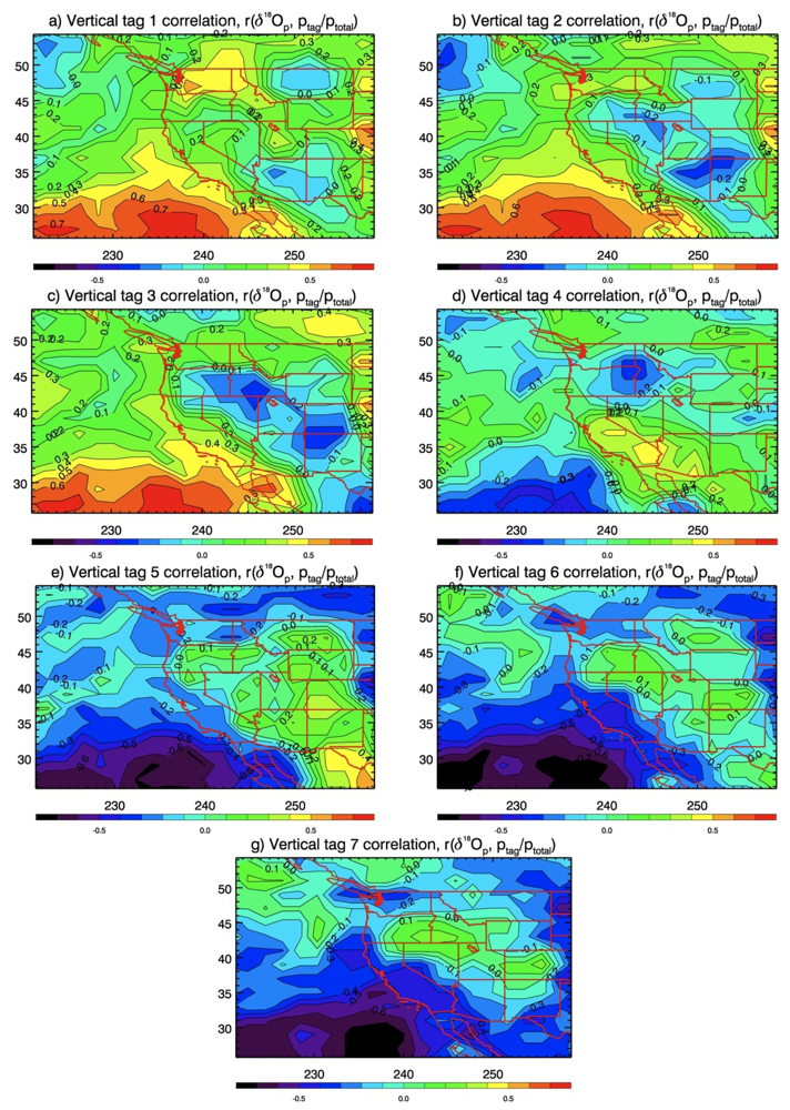
4.3.1. Circulation Effects and δ18Op

The TAGY simulation was designed to determine how interannual δ18Op variations are influenced by shifts in moisture advection from either the subtropics or middle latitudes. In TAGY, vapor was continually tagged at all 28 levels of the IsoGSM atmosphere within two boxed regions over the North Pacific: one in the subtropics and one in the middle latitudes. Outside of these two regions, the vapor tags are subject to the same atmospheric processes as normal water (i.e., advection, mixing, condensation, and rainout). As with all atmospheric General Circulation Models, IsoGSM simulates and accounts for these processes. Furthermore, since both the tagging simulation (TAGY) and the control simulation (CTRL) are nudged to the same wind and temperature fields, the water isotopologues and water tags are subject to the same atmospheric and oceanic conditions (e.g., temperature and rainout histories along air mass trajectories and ocean evaporation conditions). A fraction of the resulting simulated precipitation that falls in the western U.S. will contain the middle latitude tag and another fraction will contain the subtropical tag, which is compared to the simulated δ18O values below.
As in Subsection 4.2, interannual correlations coefficients were calculated to quantify covariance between precipitated tags and δ18Op. Figure 10a,b show the interannual correlations between δ18Op and the fraction of precipitation with the middle latitude and subtropical tags. For both tags, correlations are weak across almost all of the western U.S. This result suggests there is little covariance between interannual δ18Op variations and the fraction of precipitation advected from either the subtropics or the middle latitudes. Thus, any influence of moisture advection would be difficult to detect from δ18Op at interannual timescales. The exceptions to this include Washington and Oregon, where correlations with subtropical and middle latitude tagged precipitation fractions exceed 0.4 and −0.4, respectively. These correlations suggest that the Pacific Northwest might be a region where precipitation δ values adequately trace atmospheric circulation at interannual timescales.
To see if the correlations improve without the influence of post-condensation exchanges and condensation height, individual interannual time series of δ18Op from the NORNEV simulation were regressed against the fraction of precipitation from the bottom 7 vertical layers from the TAGZ simulations (values in Figure 6):
Water 05 01116 i001
In Equation (1), p values are simulated precipitation rates, indices i refer to each of the 7 vertical tags, and the values of Ai and B (‰) are the regression slopes and intercepts (respectively) used to fit interannually varying δ18Op from the NORNEV simulation (δNORNEV). The residual of the regression (δresidual) will have removed both the influence of post-condensation exchanges and condensation height:
Water 05 01116 i002
The interannual variations of δresidual were correlated with the fraction of precipitation from the middle latitude and subtropical regions of the TAGY simulation. The correlations between δresidual and the fraction of precipitation advected from the middle latitude-tagged region become slightly more negative (Figure 10c), which was originally the anticipated relationship. Similarly, the correlations with the fraction of precipitation with the subtropical tag significantly increased and were positive at almost all western U.S. locations (Figure 10d). For both tags, the correlations with δresidual are highest in Washington and Oregon (where the correlations already existed). These results indicate that the influence of circulation changes on δ18Op is secondary and only detectable after the removal of the primary influences of post-condensation exchanges and condensation height in California and the western U.S. interior.
Figure 10. (a) Correlation between interannual δ18Op variations and the fraction of precipitation from middle latitude tags; and (b) subtropical tags; Panels (c) and (d) show the same correlations, as (a) and (b) (respectively), but with the influence of post-condensation exchanges and condensation height removed. Contour intervals are 0.1. Absolute values of r above 0.263 are significant above the 95% confidence level.
Water 05 01116 g010

4.3.2. Circulation Effects and δ18OPW

Results from the TAGY simulation revealed that in most regions of the western U.S. the influence of circulation changes on interannual δ18Op variations is small. However, atmospheric circulation does affect the isotopic composition of vapor. Correlations between the isotopic composition of precipitable water (column integrated tropospheric vapor), δ18OPW, and the fraction of precipitable water with the middle latitude and subtropical tags are shown in Figure 11. Figure 11a reveals a strong negative correlation between δ18OPW and the mid-latitude tags throughout much of the western U.S. The strongest negative correlation in Figure 11a is located at the California/Nevada border near Lake Tahoe. However, the same figure was generated with additional tagging simulations, and it was found that the location of the strongest negative correlations was dependent on the location of boxed regions where the vapor tags were being added (figure not shown). Nonetheless, the additional simulations also revealed that the negative correlation that exists in the western U.S. is robust.
Figure 11. (a) Correlation between interannual δ18OPW variations and the fraction of precipitable water from middle latitude tags; and (b) subtropical tags. Contour intervals are 0.1. Absolute values of r above 0.263 are significant above the 95% confidence level.
Water 05 01116 g011
Correlations with the subtropical tags are positive throughout most of the western U.S. The largest correlation exists in coastal locations within Oregon and Washington, which are the same regions that had positive correlations with δ18Op. The correlations are not as high for the southwest U.S. and southern California. The additional tagging simulations revealed that the locations of the good and poor correlations in Figure 11b are robust and not dependent on the location of the boxed regions where vapor is being tagged. The robustness of both the negative correlation in Figure 11a and the positive correlation in Figure 11b indicates a strong relationship between the oxygen isotopic composition of tropospheric vapor and atmospheric circulation in the western U.S. However, this relationship was not seen in precipitation δ values in most regions because of the strong influence of post-condensation exchanges and condensation height. Indeed, the atmospheric circulation effect was only transferred to precipitation δ values in regions where variations in condensation height are relatively small like the Pacific Northwest (Figure 9).

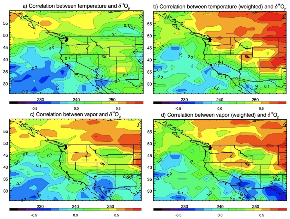
4.4. Temperature Effect

Though the NORNEV simulation demonstrated that roughly 60% of the interannual δ18Op variations were due to post-condensation exchanges throughout the western U.S., the tagging simulations discussed in Sections 4.2 and Sections 4.3 failed to describe the remaining variance in the interior states of the western U.S. Past studies [16,57] have found or suggested that regions of the interior of the U.S. show a temperature effect (positive correlations between δ18Op and local temperatures). This relationship is due to increases (decreases) in Rayleigh distillation with lower (higher) temperatures and subsequently lower (higher) δ values of vapor upon arrival at a given location. In this subsection, IsoGSM’s temperature effect relationship will be quantified within the western U.S.
The correlations between δ18Op and surface air temperature were calculated at each grid cell within the western U.S. for the CTRL simulation. Because the precipitation seasonal cycle peaks in the summer within the interior states, annual means in this subsection are calculated as the normal January to December average (though this did not change the general results). Correlations are low in the coastal areas and all of California (Figure 12a), as expected since the modeling results presented above indicated other processes drive interannual δ18Op variations. Relatively high correlations (r > 0.3) were found in an area of New Mexico spanning northward into Montana and eastern Washington (Figure 12a). The lack of high correlations between local annual mean temperatures and δ18Op reveals a problem for using climate proxies based on δ18Op values to reconstruct annual mean temperatures in the western U.S. However, when the mean temperatures are weighted by monthly precipitation the correlations significantly increase over all of the interior states of the western U.S. (Figure 12b); a result that has been found elsewhere using a different model [15]. Indeed, using precipitation-weighted temperatures increased the correlations from about 0.3 to 0.7 for many regions of the interior western U.S. These results reveal that reconstructed annual mean temperatures in the western U.S. interior could be biased towards wet season temperatures when using proxies derived from δ18Op.
Figure 12. (a,b) Correlation between δ18Op and annual mean temperature; and (c,d) surface level specific humidity (bottom panels). Right panel annual means of temperature and specific humidity were weighted by monthly precipitation. Absolute values of r above 0.263 are significant above the 95% confidence level.
Water 05 01116 g012
To demonstrate that this temperature effect in the western U.S. was a result of rainout as air masses moved through the interior of the continent, similar correlation maps were made for specific humidity (q) and precipitation-weighted specific humidity (Figure 12c,d). Though the correlation maps are not identical to the corresponding temperature plots, they both highlight the interior of the western U.S. as a region where strong correlations exist, and suggest that the simulated interannual δ18Op variations were driven by the extent of Rayleigh distillation from the coastline to the location where precipitation occurs. Thus, this rainout process gives rise to the “precipitation-weighted temperature effect”, as simulated by IsoGSM.

5. Conclusions

The modeling results suggest that interannual variations in precipitation δ values in the western U.S. are primarily caused by a combination of mechanisms, though some atmospheric processes are detectable at interannual timescales in certain regions. In the western coastal areas and almost all of California, the variations are largely controlled by changes in condensation height. These induced variations in δ18Op that account for about 20%–40% of the interannual variance, but the year-to-year changes are amplified by post-condensation exchanges, accounting for about 60% of the variance. Most of the remaining variance in California and coastal Oregon and Washington is attributable to subtropical versus middle latitude moisture advection changes (i.e., an atmospheric circulation effect), which is most prominent and detectable in the Pacific Northwest of the United States. Further north, Field et al. [58] found a similar relationship between precipitation δ values and atmospheric circulation in western Canada. In California, the atmospheric circulation effect can only be detected after the influences of post-condensation exchanges and condensation height are removed from individual time series. However, the model results suggest that atmospheric circulation is a primary influence on vapor δ values throughout almost all of the western U.S.
A temperature effect was found for the inland regions of the western U.S., such that years with anomalously cooler (warmer) temperatures will lead to more (less) isotopic rainout and lower (higher) δ values of vapor and subsequently precipitation. Like the coastal regions, these isotopic variations in δ18Op are amplified by post-condensation exchanges, contributing about 60% to the interannual variance. The δ18Op-temperature correlations found here were only large after annual mean temperatures were weighted by precipitation amounts, indicating a problem for reconstructing annual mean temperatures in the western U.S. interior.
The results presented here will help guide the interpretation of climate proxies in the western U.S. that are influenced by precipitation δ values, such as ice-cores [17,18], speleothems [21,22], tree cellulose [16,19], leaf wax n-alkanes [24,59], and lacustrine archives [25,26,27,28]. The model results suggest that climate proxy δ values from California and parts of Washington and Oregon might reflect variations in condensation height on interannual timescales. However, Washington and Oregon were also areas where δ18Op correlated with subtropical and mid-latitude tags, indicating covariance between the vertical and north-south tags in the Pacific Northwest (i.e., moisture transported from the subtropics typically rains out lower in the atmosphere). In the interior of the western U.S., proxy δ values likely trace precipitation-weighted temperatures changes, which may differ from annual mean temperatures. The TAGY tagging simulation demonstrated that vapor δ values (δ18Ov) trace atmospheric circulation over most regions of the western U.S. This particular finding may be useful in the context of the results of Helliker et al. [60] who showed through controlled experiments and model calculations that epiphyte Tillandsia usneoides from CAM plants record δ values of vapor. Thus, these plants may be useful in detecting shifts in middle latitude storm tracks [61,62]. Furthermore, the model results suggest that the Pacific Northwest is a region where δ18Op values trace atmospheric circulation, highlighting an area where shifts in storm tracks may be detectable through measurements of either precipitation or vapor δ values. Additionally, past shifts may be reconstructed through water isotope based proxy records in the Pacific Northwest. However, it is important to note that the mean circulation variations that are typical at interannual timescales (e.g., ENSO variability and the position of the North Pacific High), may differ from the type of circulation changes on longer timescales, such as multi-decadal and inter-glacial variations.
Detecting shifted storm tracks through isotope measurements should be the focus of future work, either through direct measurements of isotopes in precipitation or vapor or from climate proxy reconstructions. This is particularly important because poleward shifted middle latitude storm tracks are features of a warmer climate that almost all global climate models agree upon [61,62]. Detecting such shifts is vital for regions, like the southwest U.S., where water resources are already stressed due to an inadequate supply and growing demand. The results presented here suggest that storm track shifts can be detected through ongoing monitoring of δ18Op in the Pacific Northwest. This stresses the need to continue station observations of the isotopic composition of precipitation at sites in Oregon and Washington (e.g., the Olympic site from Buenning et al. [37]). Furthermore, ongoing measurements of isotopes in vapor may serve useful at detecting storm track shifts in the western US, either from satellite retrievals [63,64,65] or ground-based remote sensing [66]. The modeling results presented here demonstrate how moisture advection can influence the isotopes in atmospheric moisture in the western U.S.; thus, future work should focus on developing isotope-based methodologies to monitor and detect storm track variability over the western U.S.

Acknowledgments

Funding for this work was provided by the NOAA/CPO Climate Change & Detection Program: Paleoclimate Studies (grant NA10OAR4310129). This work was also supported by a grant from the National Science Foundation (award AGS-1049238). We also thank the helpful comments and suggestions from two anonymous reviewers.

Conflict of Interest

The authors declare no conflict of interest.

References

  1. Lorius, C.; Jouzel, J.; Raynaud, D.; Hansen, J.; Letreut, H. The ice-core record: Climate sensitivity and future greenhouse warming. Nature 1990, 347, 139–145. [Google Scholar] [CrossRef]
  2. Vimeux, F.; Ginot, P.; Schwikowski, M.; Vuille, M.; Hoffmann, G.; Thompson, L.G.; Schotterer, U. Climate variability during the last 1000 years inferred from Andean ice cores: A review of methodology and recent results. Palaeogeogr. Palaeocl. 2009, 281, 229–241. [Google Scholar] [CrossRef]
  3. McDermott, F. Palaeo-climate reconstruction from stable isotope variations in speleothems: A review. Quat. Sci. Rev. 2004, 23, 901–918. [Google Scholar] [CrossRef]
  4. Sternberg, L.D.L.O. Oxygen stable isotope ratios of tree-ring cellulose: The next phase of understanding. New Phytol. 2009, 181, 553–562. [Google Scholar] [CrossRef]
  5. Dansgaard, W. Stable isotopes in precipitation. Tellus 1964, 16, 436–468. [Google Scholar] [CrossRef]
  6. Araguas-Araguas, L.; Froehlich, K.; Rozanski, K. Stable isotope composition of precipitation over southeast Asia. J. Geophys. Res. Atmos. 1998, 103, 28721–28742. [Google Scholar] [CrossRef]
  7. Yamanaka, T.; Shimada, J.; Hamada, Y.; Tanaka, T.; Yang, Y.H.; Zhang, W.J.; Hu, C.S. Hydrogen and oxygen isotopes in precipitation in the northern part of the North China Plain: Climatology and inter-storm variability. Hydrol. Process. 2004, 18, 2211–2222. [Google Scholar] [CrossRef]
  8. Risi, C.; Bony, S.; Vimeux, F. Influence of convective processes on the isotopic composition (δ18O and δD) of precipitation and water vapor in the tropics: 2. Physical interpretation of the amount effect. J. Geophys. Res. Atmos. 2008, 113, D19306. [Google Scholar] [CrossRef]
  9. Lee, J.E.; Fung, I. “Amount effect” of water isotopes and quantitative analysis of post-condensation processes. Hydrol. Process. 2008, 22, 1–8. [Google Scholar] [CrossRef]
  10. Lee, J.E.; Risi, C.; Fung, I.; Worden, J.; Scheepmaker, R.A.; Lintner, B.; Frankenberg, C. Asian monsoon hydrometeorology from TES and SCIAMACHY water vapor isotope measurements and LMDZ simulations: Implications for speleothem climate record interpretation. J. Geophys. Res. Atmos. 2012, 117, D15112. [Google Scholar]
  11. Field, R.D.; Jones, D.B.A.; Brown, D.P. Effects of postcondensation exchange on the isotopic composition of water in the atmosphere. J. Geophys. Res. Atmos. 2010, 115, D24305. [Google Scholar] [CrossRef]
  12. Buenning, N.H.; Noone, D.C.; Riley, W.J.; Still, C.J.; White, J.W.C. Influences of the hydrological cycle on observed interannual variations in atmospheric CO18O. J Geophys. Res. Biogeo. 2011, 116, G04001. [Google Scholar] [CrossRef]
  13. Rozanski, K.; Sonntag, C.; Munnich, K.O. Factors controlling stable isotope composition of european precipitation. Tellus 1982, 34, 142–150. [Google Scholar] [CrossRef]
  14. Bowen, G.J. Spatial analysis of the intra-annual variation of precipitation isotope ratios and its climatological corollaries. J. Geophys. Res. Atmos. 2008, 113, D05113. [Google Scholar] [CrossRef]
  15. Sturm, C.; Zhang, Q.; Noone, D. An introduction to stable water isotopes in climate models: Benefits of forward proxy modelling for paleoclimatology. Clim. Past 2010, 6, 115–129. [Google Scholar] [CrossRef]
  16. Berkelhammer, M.; Stott, L.D. Secular temperature trends for the southern Rocky Mountains over the last five centuries. Geophys. Res. Lett. 2012, 39, L17701. [Google Scholar]
  17. Naftz, D.L.; Susong, D.D.; Schuster, P.F.; Cecil, L.D.; Dettinger, M.D.; Michel, R.L.; Kendall, C. Ice core evidence of rapid air temperature increases since 1960 in alpine areas of the Wind River Range, Wyoming, United States. J. Geophys. Res. Atmos. 2002, 107, ACL 3. [Google Scholar]
  18. Schuster, P.F.; White, D.E.; Naftz, D.L.; Cecil, L.D. Chronological refinement of an ice core record at Upper Fremont Glacier in south central North America. J. Geophys. Res. Atmos. 2000, 105, 4657–4666. [Google Scholar] [CrossRef]
  19. Berkelhammer, M.; Stott, L.D. Modeled and observed intra-ring δ18O cycles within late Holocene Bristlecone Pine tree samples. Chem. Geol. 2009, 264, 13–23. [Google Scholar] [CrossRef]
  20. Berkelhammer, M.B.; Stott, L.D. Recent and dramatic changes in Pacific storm trajectories recorded in δ18O from Bristlecone Pine tree ring cellulose. Geochem. Geophys. Geosy. 2008, 9, Q04008. [Google Scholar]
  21. Vacco, D.A.; Clark, P.U.; Mix, A.C.; Cheng, H.; Edward, R.L. A speleothem record of Younger Dryas cooling, Klamath Mountains, Oregon, USA. Quat. Res. 2005, 64, 249–256. [Google Scholar] [CrossRef]
  22. Oster, J.L.; Montanez, I.P.; Sharp, W.D.; Cooper, K.M. Late Pleistocene California droughts during deglaciation and Arctic warming. Earth Planet Sci. Lett. 2009, 288, 434–443. [Google Scholar] [CrossRef]
  23. Ersek, V.; Clark, P.U.; Mix, A.C.; Cheng, H.; Edwards, R.L. Holocene winter climate variability in mid-latitude western North America. Nat. Commun. 2012, 3. [Google Scholar] [CrossRef]
  24. Feakins, S.J.; Sessions, A.L. Controls on the D/H ratios of plant leaf waxes in an arid ecosystem. Geochim. Cosmochim. Acta 2010, 74, 2128–2141. [Google Scholar] [CrossRef]
  25. Benson, L.V.; Burdett, J.W.; Kashgarian, M.; Lund, S.P.; Phillips, F.M.; Rye, R.O. Climatic and hydrologic oscillations in the Owens Lake basin and adjacent Sierra Nevada, California. Science 1996, 274, 746–749. [Google Scholar] [CrossRef]
  26. Benson, L.V.; Lund, S.P.; Burdett, J.W.; Kashgarian, M.; Rose, T.P.; Smoot, J.P.; Schwartz, M. Correlation of late-Pleistocene lake-level oscillations in Mono Lake, California, with North Atlantic climate events. Quat. Res. 1998, 49, 1–10. [Google Scholar] [CrossRef]
  27. Li, H.C.; Ku, T.L. Delta C-13-delta O-18 covariance as a paleohydrological indicator for closed-basin lakes. Palaeogeogr. Palaeoclimatol. 1997, 133, 69–80. [Google Scholar] [CrossRef]
  28. Li, H.C.; Ku, T.L.; Stott, L.D.; Anderson, R.F. Stable isotope studies on Mono Lake (California). 1. Delta O-18 in lake sediments as proxy for climatic change during the last 150 years. Limnol. Oceanogr. 1997, 42, 230–238. [Google Scholar]
  29. Coplen, T.B.; Neiman, P.J.; White, A.B.; Landwehr, J.M.; Ralph, F.M.; Dettinger, M.D. Extreme changes in stable hydrogen isotopes and precipitation characteristics in a landfalling Pacific storm. Geophys. Res. Lett. 2008, 35, L21808. [Google Scholar] [CrossRef]
  30. Yoshimura, K.; Kanamitsu, M.; Dettinger, M. Regional downscaling for stable water isotopes: A case study of an atmospheric river event. J. Geophys. Res. Atmos. 2010, 115, D18114. [Google Scholar] [CrossRef]
  31. Vachon, R.W.; Welker, J.M.; White, J.W.C.; Vaughn, B.H. Monthly precipitation isoscapes δ18O of the United States: Connections with surface temperatures, moisture source conditions, and air mass trajectories. J. Geophys. Res. Atmos. 2010, 115, D21126. [Google Scholar]
  32. Ersek, V.; Mix, A.C.; Clark, P.U. Variations of delta O-18 in rainwater from southwestern Oregon. J. Geophys. Res. Atmos. 2010, 115, D09109. [Google Scholar] [CrossRef]
  33. Friedman, I.; Harris, J.M.; Smith, G.I.; Johnson, C.A. Stable isotope composition of waters in the Great Basin, United States—1. Air-mass trajectories. J. Geophys. Res. Atmos. 2002, 107. [Google Scholar] [CrossRef]
  34. Friedman, I.; Smith, G.I.; Gleason, J.D.; Warden, A.; Harris, J.M. Stable Isotope Composition of Waters in Southeastern California. 1. Modern Precipitation. J. Geophys. Res. Atmos. 1992, 97, 5795–5812. [Google Scholar] [CrossRef]
  35. Friedman, I.; Smith, G.I.; Johnson, C.A.; Moscati, R.J. Stable isotope compositions of waters in the Great Basin, United States—2. Modern precipitation. J. Geophys. Res. Atmos. 2002, 107. [Google Scholar] [CrossRef]
  36. Berkelhammer, M.; Stott, L.; Yoshimura, K.; Johnson, K.; Sinha, A. Synoptic and mesoscale controls on the isotopic composition of precipitation in the western United States. Clim. Dynam. 2012, 38, 433–454. [Google Scholar] [CrossRef]
  37. Buenning, N.H.; Stott, L.; Yoshimura, K.; Berkelhammer, M. The cause of the seasonal variation in the oxygen isotopic composition of precipitation along the western U.S. coast. J. Geophys. Res. Atmos. 2012, 117, D18114. [Google Scholar]
  38. Yoshimura, K.; Kanamitsu, M.; Noone, D.; Oki, T. Historical isotope simulation using Reanalysis atmospheric data. J. Geophys. Res. Atmos. 2008, 113, D19108. [Google Scholar] [CrossRef]
  39. Reynolds, R.W.; Smith, T.M. Improved global sea-surface temperature analyses using optimum interpolation. J. Climate 1994, 7, 929–948. [Google Scholar] [CrossRef]
  40. Kalnay, E.; Kanamitsu, M.; Kistler, R.; Collins, W.; Deaven, D.; Gandin, L.; Iredell, M.; Saha, S.; White, G.; Woollen, J.; et al. The NCEP/NCAR 40-year reanalysis project. Bull. Amer. Meteorol. Soc. 1996, 77, 437–471. [Google Scholar] [CrossRef]
  41. Yoshimura, K.; Kanamitsu, M. Dynamical global downscaling of global reanalysis. Mon. Weather Rev. 2008, 136, 2983–2998. [Google Scholar] [CrossRef]
  42. Majoube, M. Fractionation in O-18 between ice and water vapor. J. Chim. Phys. Phys. Chim. Biol. 1971, 68, 625–636. [Google Scholar]
  43. Majoube, M. Oxygen-18 and deuterium fractionation between water and steam. J. Chim. Phys. Phys. Chim. Biol. 1971, 68, 1423–1436. [Google Scholar]
  44. Merlivat, L.; Jouzel, J. Global climatic interpretation of the deuterium-oxygen-18 relationship for precipitation. J. Geophys. Res. 1979, 84, 5029–5033. [Google Scholar] [CrossRef]
  45. Jouzel, J.; Merlivat, L. Deuterium and oxygen 18 in precipitation: Modeling of the isotopic effects during snow formation. J. Geophys. Res. 1984, 89, 11749–11757. [Google Scholar] [CrossRef]
  46. Stewart, M.K. Stable isotope fractionation due to evaporation and isotopic-exchange of falling waterdrops—Applications to atmospheric processes and evaporation of lakes. J. Geophys. Res. 1975, 80, 1133–1146. [Google Scholar] [CrossRef]
  47. Bony, S.; Risi, C.; Vimeux, F. Influence of convective processes on the isotopic composition (δ18O and δD) of precipitation and water vapor in the tropics: 1. Radiative-convective equilibrium and Tropical Ocean-Global Atmosphere-Coupled Ocean-Atmosphere Response Experiment (TOGA-COARE) simulations. J. Geophys. Res. Atmos. 2008, 113, D19305. [Google Scholar] [CrossRef]
  48. Wright, J.S.; Sobel, A.H.; Schmidt, G.A. Influence of condensate evaporation on water vapor and its stable isotopes in a GCM. Geophys. Res. Lett. 2009, 36, L12804. [Google Scholar] [CrossRef]
  49. Feng, X.H.; Reddington, A.L.; Faiia, A.M.; Posmentier, E.S.; Shu, Y.; Xu, X.M. The Changes in North American atmospheric circulation patterns indicated by wood cellulose. Geology 2007, 35, 163–166. [Google Scholar] [CrossRef]
  50. Zhu, M.F.; Stott, L.; Buckley, B.; Yoshimura, K. 20th century seasonal moisture balance in Southeast Asian montane forests from tree cellulose δ18O. Climatic Change 2012, 115, 505–517. [Google Scholar] [CrossRef]
  51. Zhu, M.F.; Stott, L.; Buckley, B.; Yoshimura, K.; Ra, K. Indo-Pacific Warm Pool convection and ENSO since 1867 derived from Cambodian pine tree cellulose oxygen isotopes. J. Geophys. Res. Atmos. 2012, 117, D11307. [Google Scholar] [CrossRef]
  52. Roden, J.S.; Lin, G.G.; Ehleringer, J.R. A mechanistic model for interpretation of hydrogen and oxygen isotope ratios in tree-ring cellulose. Geochim. Cosmochim. Acta 2000, 64, 21–35. [Google Scholar] [CrossRef]
  53. Kanner, L.; Buenning, N.H.; Stott, L.; Stahle, D. Climatologic and hydrologic influences on the oxygen isotope ratio of tree cellulose in coastal southern California during the late 20th century. Geochem. Geophys. Geosy. 2013. Submitted for publiation. [Google Scholar]
  54. Risi, C.; Noone, D.; Worden, J.; Frankenberg, C.; Stiller, G.; Kiefer, M.; Funke, B.; Walker, K.; Bernath, P.; Schneider, M.; et al. Process-evaluation of tropospheric humidity simulated by general circulation models using water vapor isotopologues: 1. Comparison between models and observations. J. Geophys. Res. Atmos. 2012, 117, D05303. [Google Scholar] [CrossRef]
  55. Ehhalt, D.H.; Rohrer, F.; Fried, A. Vertical profiles of HDO/H2O in the troposphere. J. Geophys. Res. Atmos. 2005, 110, D13301. [Google Scholar] [CrossRef]
  56. Sayres, D.S.; Pfister, L.; Hanisco, T.F.; Moyer, E.J.; Smith, J.B.; St Clair, J.M.; OʼBrien, A.S.; Witinski, M.F.; Legg, M.; Anderson, J.G. Influence of convection on the water isotopic composition of the tropical tropopause layer and tropical stratosphere. J. Geophys. Res. Atmos. 2010, 115, D00J20. [Google Scholar] [CrossRef]
  57. Vachon, R.W.; White, J.W.C.; Gutmann, E.; Welker, J.M. Amount-weighted annual isotopic δ18O values are affected by the seasonality of precipitation: A sensitivity study. Geophys. Res. Lett. 2007, 34, L21707. [Google Scholar] [CrossRef]
  58. Field, R.D.; Moore, G.W.K.; Holdsworth, G.; Schmidt, G.A. A GCM-based analysis of circulation controls on δ18O in the southwest Yukon, Canada: Implications for climate reconstructions in the region. Geophys. Res. Lett. 2010, 37, L05706. [Google Scholar]
  59. Romero, I.C.; Feakins, S.J. Spatial gradients in plant leaf wax D/H across a coastal salt marsh in southern California. Org. Geochem. 2011, 42, 618–629. [Google Scholar] [CrossRef]
  60. Helliker, B.R. On the controls of leaf-water oxygen isotope ratios in the atmospheric crassulacean acid metabolism epiphyte tillandsia usneoides. Plant Physiol. 2011, 155, 2096–2107. [Google Scholar] [CrossRef]
  61. Yin, J.H. A consistent poleward shift of the storm tracks in simulations of 21st century climate. Geophys. Res. Lett. 2005, 32, L18701. [Google Scholar] [CrossRef]
  62. Salathe, E.P. Influences of a shift in North Pacific storm tracks on western North American precipitation under global warming. Geophys. Res. Lett. 2006, 33, L19820. [Google Scholar] [CrossRef]
  63. Worden, J.; Bowman, K.; Noone, D.; Beer, R.; Clough, S.; Eldering, A.; Fisher, B.; Goldman, A.; Gunson, M.; Herman, R.; et al. Tropospheric emission spectrometer observations of the tropospheric HDO/H2O ratio: Estimation approach and characterization. J. Geophys. Res. Atmos. 2006, 111, D16309. [Google Scholar] [CrossRef]
  64. Worden, J.; Noone, D.; Bowman, K.; Spect, T.E. Importance of rain evaporation and continental convection in the tropical water cycle. Nature 2007, 445, 528–532. [Google Scholar] [CrossRef]
  65. Frankenberg, C.; Yoshimura, K.; Warneke, T.; Aben, I.; Butz, A.; Deutscher, N.; Griffith, D.; Hase, F.; Notholt, J.; Schneider, M.; et al. Dynamic processes governing lower-tropospheric HDO/H2O ratios as observed from space and ground. Science 2009, 325, 1374–1377. [Google Scholar] [CrossRef]
  66. Wunch, D.; Toon, G.C.; Wennberg, P.O.; Wofsy, S.C.; Stephens, B.B.; Fischer, M.L.; Uchino, O.; Abshire, J.B.; Bernath, P.; Biraud, S.C.; et al. Calibration of the total carbon column observing network using aircraft profile data. Atmos. Meas. Tech. 2010, 3, 1351–1362. [Google Scholar] [CrossRef]

