Article

Expansion of an Existing Water Management Model for the Analysis of Opportunities and Impacts of Agricultural Irrigation under Climate Change Conditions

1
Institute of Landscape Hydrology, Leibniz Centre for Agricultural Landscape Research (ZALF), Eberswalder Straße 84, Müncheberg D-15374, Germany
2
Institute of Socio-Economics, Leibniz Centre for Agricultural Landscape Research (ZALF), Eberswalder Straße 84, Müncheberg D-15374, Germany
*
Author to whom correspondence should be addressed.
Submission received: 26 August 2015 / Revised: 3 November 2015 / Accepted: 5 November 2015 / Published: 11 November 2015

Abstract

:
The impact of climate change and increased irrigation area on future hydrologic and agro-economic conditions was analysed for a representative basin in northeastern Germany using an expanded version of the WBalMO (water balance model) for water management. The model expansion represents various temporally and spatially differentiated irrigation water use processes, including agricultural irrigation, as part of a river basin’s water management. We show that climate changes lead to increased irrigation water demands in the future, which will not always be able to be met. The resulting water deficits were shown for different crops depending on their irrigation priority and the water available. With an increased irrigation area, water deficits will rise. This may limit the profitability of agricultural irrigation. The impacts of climate change on low-flow conditions in the river are much higher than those of the increase in irrigated area alone. Therefore, any additional increases of irrigation will require careful monitoring of water availability to avoid critical impacts on river flows. The expanded model was able to replicate the processes of agricultural irrigation water use and can thus be used to test the impact of policies such as the certification of new irrigation permits.

1. Introduction

Even though water is not generally scarce for agricultural irrigation in Germany at the national level, some shortages occasionally arise at the regional level and seasonally. These problems occur in some regions due to highly concentrated agricultural or horticultural activities, often historically based or as a result of large processing units [1]. In the eastern part of Germany, an irrigation infrastructure was maintained until 1990 in an effort to secure yield stability in order to be less dependent on food imports linked to high foreign currency expenses [2]. After the political changes, this infrastructure was removed to a large extent. Recently, farms in some regions have reinvested, and agricultural areas being irrigated are increasing once again [3]. Nevertheless, particularly in northeastern Germany, water use in agricultural crop production needs to be balanced against the groundwater recharge, which also is important for water supply in urban areas, minimum environmental flow in streams or peat protection in wetlands [4].
In this region, with its more continental climate, drought stress during the cropping season is one of the main yield and quality-limiting factors [5]. Holsten et al. [6] even postulated a significant decrease in the average annual available soil water content in the future for the Federal State of Brandenburg (northeastern Germany). Widespread sandy soils with low capacities of water retention aggravate the situation [7]. Increasing dry periods caused by climate change may result in even longer and more severe shortages in water availability for plants [8,9].
Against this background, an increase in agricultural irrigation is a likely adaptation measure to cope with climate change in drought-prone regions of northern and eastern Germany [1]. Additionally, economic forecasts for agricultural markets encourage farmers to invest in irrigation systems: potentially higher crop prices in the future induced by higher international demand will make investments in irrigation technology even more profitable [10]. This trend is strengthened even further by incentives for biofuels and biogas production [11] and financial support for irrigation technology through the European Union rural development plans (RDPs) [12].
Although Gutzler et al. [13] argue that Brandenburg generally has an adequate water supply, concerns exist that an increased level of irrigation may lead to severe impacts on individual ground water supplies as well as on surface water bodies. An insufficient ground water supply available for other users could be the consequence, and the low flows of stream systems could be affected [14,15]. In addition, climate change could also increase the impacts of agricultural production on water quality and additional ecological parameters, such as in lakes [16].
The amount of irrigated agricultural land—and thus the demand for irrigation water—has been increasing over the past 20 years [3]. Therefore, water authorities now issue water withdrawal permits with the stipulation that regional water resources are not negatively influenced. These permits are based on a currently sufficient water availability. However, this water availability is calculated based on past experience. This calculation therefore neglects the aspect of global warming, which may lead to decreasing groundwater recharge [17] or increasing low flow conditions in rivers and streams [18], and probably higher demand for irrigation water. This poses the risk of an overuse of water resources.
As a result, if conflicts between the benefits and consequences of increasing irrigation in the landscape intensify, regulatory authorities will need to make difficult decisions. They will require tools to help them make an informed decision. From the perspective of systems theory, this is a multi-criteria, stochastic optimisation problem which requires the involvement of multiple decision-makers. Methods and models of water management have been reinforced in the past to solve such problems with a multitude of solutions [19]. Scenario analyses have been suitable in combination with stochastic methods to cope with the uncertainties of future climate and water yields [20].
Several agencies in Germany, particularly in Brandenburg, use WBalMo (water balance model) as a standard model for planning and managing water resource systems. WBalMo is a water management model that simulates water use processes on the level of the river basin and can be used to carry out such analyses [21,22,23]. WBalMo also provides capabilities for model expansions; some authors have used this model to present results on topics similar to those treated in this study by developing and using model expansion modules. Dietrich, Redetzky and Schwarzel [24] developed a module for the WBalMo model that simulates the water budget of wetlands. They applied this module to investigate the effects of water scarcity at shallow water table sites in use for agriculture. Dietrich et al. [25] investigated the impact of climate change on the Spreewald wetland water budget in scenario analyses; Grossmann and Dietrich [26,27] expanded and applied the WBalMo model to investigate the social and economic issues of a climate change scenario.
However, the basic version of WBalMo can only be used to examine agricultural irrigation relative to the amount of water withdrawal permits. Actual meteorological conditions and physiological requirements are not taken into account when determining an irrigation demand depending on the meteorological boundary conditions. Thus, a serious assessment of the impact of climate change on the demand, impacts and economic results of irrigation is virtually impossible with the current basic version.
Because of this, we developed a WBalMo expansion which would allow more realistic statements on water demand versus water availability, as well as comparing the agricultural benefits of an increased area of field irrigation with potential consequences of climate change [28]. Our scenario-driven approach uses irrigation demand as an independent variable based on individual farmer behaviour. We assume that farmers will use irrigation water as long as the variable costs for irrigation are covered and water is available, once they have invested in an irrigation system with the expectation of beneficial economic conditions.
The objective of our paper is to present an expansion for the WBalMo water resources management model. The expansion improves assessments of water withdrawal by agricultural irrigation systems in the context of the complex water use processes in a river basin dependent on meteorological conditions, systems of crop irrigation, and the amount of irrigated land. It was tested with an available WBalMo model of a representative basin in the northeastern German Federal State of Brandenburg. The results include an evaluation of the economic effects as well as the ecological effects on the flow situation in the river system of the basin. We used the model to investigate the impact of climate change effects and increased irrigation area in this region on water resources. Based on our findings, we draw conclusions for future adaptations of water management strategies.

2. Methods and Materials

2.1. Determination of Agricultural Irrigation Water Demand and Water Use in a River Basin

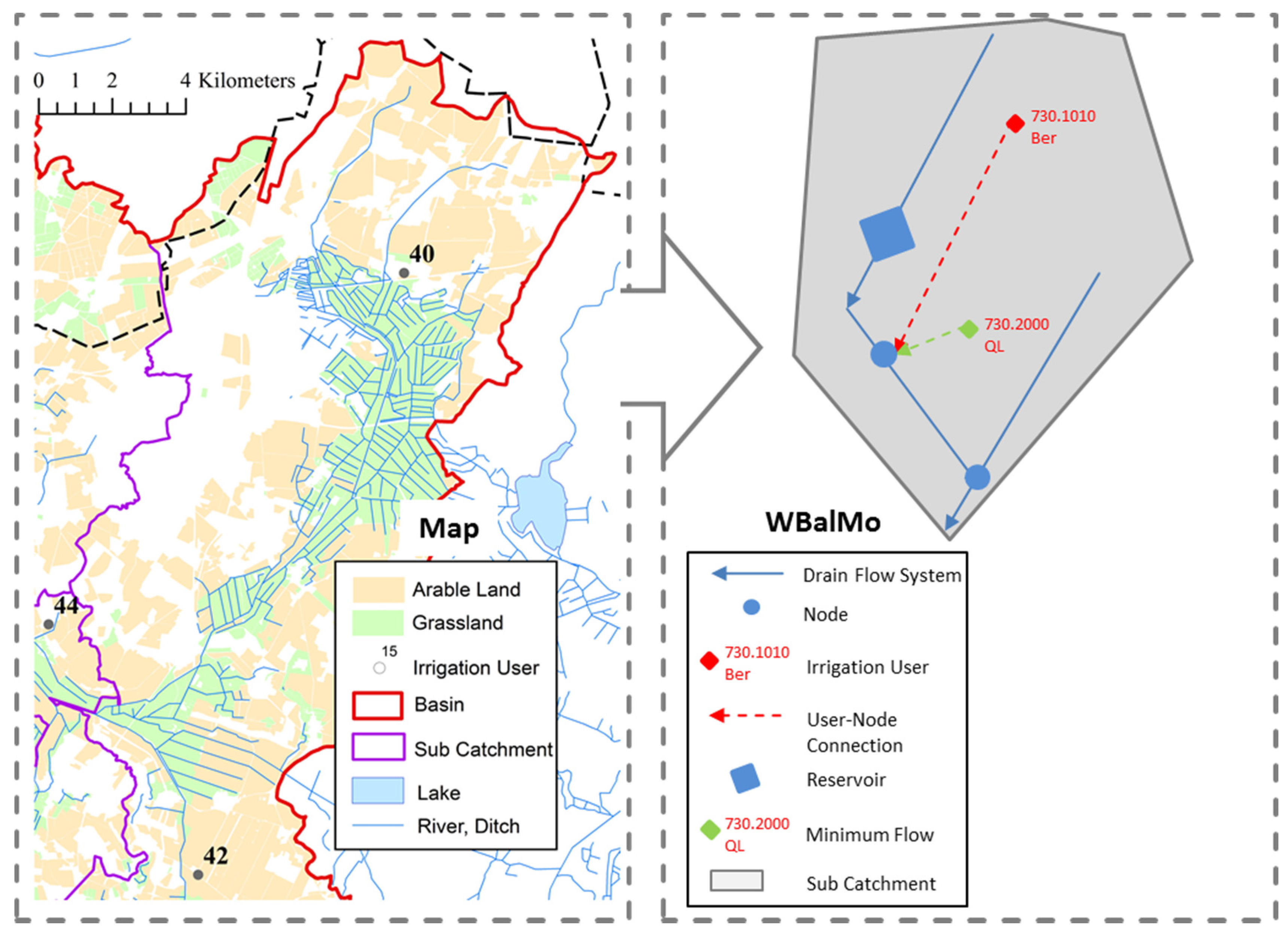
2.1.1. The WBalMo Water Management Model

The WBalMo water management model uses stochastically simulated time series of meteorological and discharge data as input for the deterministic simulation of water use processes to solve problems of water availability and water distribution to different water users at the river basin scale [21]. The model works on the basis of monthly time intervals. It is usually used to demonstrate the outcomes of various water resources management options when attempting to achieve expected water management targets. A water resources management option describes all relevant control actions of water use in a basin, such as reservoir management and industrial or agricultural water withdrawals and returns.
The model input parameters, such as precipitation, potential evapotranspiration and discharge, are based on measured meteorological and discharge data time series. Multivariate auto-regression methods are used to generate a large number of realisations of the input values based on these measured data time series [29,30,31]. In addition, a stochastic discharge data time series can be generated using hydrological models with meteorological data time series of climate models [32]. A large number of time series is a precondition for an accurate statistical evaluation of the consequences of a chosen water resources management concept.
In WBalMo the complex tributary system of a river basin is represented by a simplified system of flowing water. The river basin is subdivided into sub-catchments. Nodes are positioned at points where water flows together and adds the discharge of different stream segments. Additional nodes can be implemented to connect the stream system with sub-catchments, water management elements (e.g., reservoirs), or a specific water user (Figure 1). Each of these nodes can handle the water supply, and the relevant water users’ demands and withdrawals, as well as other related water management options, such as reservoir management or minimal environmental flows in streams. The distribution of water to each user is handled by a priority system. The priority system normally follows the natural flow direction in the running water system, but it may also deviate from it. A user with a lower priority has fewer chances to receive his water demand compared to one with a higher priority. Moreover, water withdrawal permits for water users (farms as well as non-agricultural water users) can be evaluated in order to limit water withdrawals to the amount approved.
One important parameter of water management is the water demand of different types of water users. In the classic approach, the water permits are used to determine the water demand of each user. This approach is not able to consider changing conditions affecting real water demand. This is a main reason different modules have been developed to use WBalMo in special applications. Dietrich et al. [25] developed a module for the calculation of water demand in shallow water table sites in relation to actual site conditions; Koch and Voegele [33] estimate the demand for cooling water in power plants in relation to power plant technology. In the existing applications of WBalMo agricultural irrigation has only been examined using the actual permits farms received from water authorities in the past. Section 2.1.2 outlines a model expansion that calculates the water demand of crops in relation to the site conditions in the actual time interval and aggregates the demand of all sub-areas into demand of all water users who are connected to a WBalMo node.
The deterministic simulation of the water use processes described above for large number stochastic simulated realisations and the registration of all relevant parameters enables a statistical evaluation of the results [34]. Such information can include hydrological parameters, yields or costs [25,26,27,33].
Figure 1. Scheme of the transmission of the drain flow system, water users and other information relevant for water management into the WBalMo model structure.
Water 07 06351 g001

2.1.2. Implementation of an Agricultural Irrigation Module in the Model WBalMo

In the original WBalMo, agricultural irrigation water users are represented with water demand equal to their water withdrawal permits. In our investigation WBalMo should allow more realistic statements on consequences relevant for water management, such as water availability for downstream water users or low flows, as well as agricultural benefits such as an increase in crop yield, and contingent costs, as well as additional revenue through irrigation considering climate change. For this, we developed an expansion module for WBalMo describing water demand and availability (Figure 2) as well as the revenue from agricultural irrigation. The basic equations implemented in the code routines of this module are described below.
User u can irrigate several crops c in an area A u , c . The soil’s water retention capacity in the model only covers the available water capacity Θ a u , c . Each user’s crops are assigned Θ a u , c depending on the soil in which the crop is grown. The soil can only be irrigated within a range of soil water content from Θ Start u , c up to Θ Stop u , c ; this must be defined for all users and crops. Under the assumption that this water retention capacity is completely filled at the beginning of each March, the soil water budget is calculated from March until October.
Figure 2. Outline showing how agricultural irrigation water demand is determined for a crop.
Water 07 06351 g002
The soil water content Θ u , c , m 0 which is expected at the end of a month m without irrigation is calculated from precipitation P m   and usable soil water Θ u , c , m 1 from the month before minus crop evapotranspiration ET u , c , m (Figure 2).
Θ u , c , m 0 =  P m    K c m   · ET ref m + Θ u , c , m 1
If,
Θ u , c , m 0 > Θ a u , c ,   Θ u , c , m 0 =  Θ a u , c ;
Θ u , c , m 0 < 0 ,   Θ u , c , m 0 = 0
To estimate crop evapotranspiration, the approach described in the FAO’s Irrigation and Drainage Paper No. 56 [35] was chosen, calculating crop evapotranspiration from the reference evapotranspiration ET ref m and crop coefficient K c m . The crop coefficients were defined based on [35], taking into account regional values for crops [36,37] for every month and possible (i.e., agriculturally effective) irrigation over the growing season (Table 1).
Table 1. Crop coefficients for the months ( K c m ) of the vegetation period and the months with possible irrigation (dark background).
CropMarchAprilMayJuneJulyAugust
Winter wheat1.071.121.361.361.31-
Winter rye1.011.071.421.311.26-
Winter barley1.121.181.541.411.36-
Winter rapeseed1.011.181.601.361.11
Silage maize-0.240.540.791.110.91
Potatoes-0.591.071.111.411.21
Oats-0.831.301.411.36-
Asparagus0.470.59-0.431.311.31
If the soil water content Θ u , c , m 0 at the end of a month is smaller than the initial water content for irrigation  Θ Start u , c , an irrigation water demand D irr u , c , m arises, which is calculated using the following Equation:
D i r r u , c , m = ( Θ s t a r t u , c Θ u , c , m 0 ) · ( 1 + k v u , c )
The water demand can additionally increase due to losses that depend on the technique of irrigation used. This can be evaluated using the loss coefficient k v u , c . At the end, the irrigation water demand of each irrigation water user is aggregated for his crops:
D i r r u , m = c = 1 c n D i r r u , c , m
The water user’s water demand must be compared with the water available at the water withdrawal node. To check this, the routine for user water availability of the basic WBalMo-kernel, which contains the code routines for calculation and controlling the simulation, is used (Figure 3). Here, availability is limited by the water supply and water withdrawals by users with higher priorities (e.g., minimum ecological flows) as well as the users’ water permits. The withdrawal will be limited if water demand is higher than the permissible withdrawal. At the end of the interval, each water user receives a supply depending on his demand and the availability at his node.
Figure 3. Flowchart of the agricultural irrigation module and its interaction with the WBalMo−kernel.
Water 07 06351 g003
In the next step the irrigation module distributes the irrigation water available to a user to his crops according to a priority list (Table 2). These priorities are determined by the crop’s profitability. For example, maize is ranked higher than winter wheat, due to its likely use as raw material in highly profitable biogas plants. In dry years, a user’s irrigation water demand may exceed the amount of water available. In such cases the low-priority crops cannot be irrigated, or can only be irrigated inadequately.
Table 2. Crop irrigation priorities and water productivity coefficients.
CropPriorityWater Productivity Coefficient (kg·ha−1·mm−1)
Asparagus125
Potatoes2120
Silage maize3120
Winter wheat415
Winter barley512
Winter rye615
Winter rapeseed79
Oats817
Depending on the actual irrigation water withdrawal and its assignment to crop W irr u , c , m , the soil water content Θ u , c , m at the end of a given month can be calculated using the following equation:
Θ u , c , m = Θ u , c , m 0 + W irr u , c , m ( 1 + k v u , c )
Afterwards, we can calculate the irrigation water deficit for crop Def irr u , c , m between water demand D irr u , c , m and water withdrawal W irr u , c , m and as the sum of all the crops for a user as follows:
D e f i r r u , c , m = D i r r u , c , m W i r r u , c , m
D e f i r r u , m = c = 1 c n D e f i r r u , c , m
The additional crop yield based on irrigation Y u , c , y has been calculated as the annual sum of the actual monthly withdrawal of irrigation water for crop W irr u , c , y using water productivity coefficient k Y c for the yield of each crop (Equation (7)).
However, this approach assumes linearity in the crop/water relationship. This is possible if the water productivity coefficients are adapted to the irrigation technology and management applied. Table 2 contains examples of values of these coefficients for irrigation in the months of appropriate irrigation (see Table 1), with the start of an irrigation event from Θ Start u , c = 40% up to Θ Stop u , c = 80% with sprinkler irrigation. The coefficients used were taken from the literature [38] (see Table 2).
Y u , c , y = ( m = 1 n m W i r r u , c , m , y ) · k Y c
This annual additional crop yield with irrigation was multiplied by the price coefficient k P c to obtain the additional revenue irr c that can be achieved through the irrigation of a crop:
revenue i r r c = k P c · Y u , c , y
Crop price coefficients are taken from previous literature [39]. Costs for irrigation C u , c , y are calculated as the total costs per unit of irrigation water for a crop, including fixed and variable costs for water provision as follows:
C u , c , y = ( m = 1 n m W i r r u , c , m , y ) · k C c
Cost coefficients k C c were distinguished per user as well as by the surface and groundwater sources. Average costs were also taken from preceding literature [40].

2.2. Study Area and Model Setup

2.2.1. Description of Study Area

We tested the module of the WBalMo model in the Nuthe river basin, which is located in the administrative districts of Potsdam-Mittelmark, Dahme-Spreewald and Teltow-Flaeming. These districts are reported to have the highest intensities of agricultural irrigation in the Federal State of Brandenburg (about 8372 hectares of irrigation land under irrigation in total) [41]. This area is characterised by the most intensive potato and vegetable production in the entire state. Additionally, many biogas plants use maize silage as a fermentation substrate (Integrated Administration and Control System of the European Commission (IACS) [42]).
The Nuthe river basin catchment covers an area of 180,600 hectares (Figure 4). It is located in the transition zone between a maritime and a continental climate, with an annual precipitation of 568 mm·year−1, an average annual air temperature of 9.5 °C and an FAO grass reference evapotranspiration of about 642 mm·year−1 (means of series 1991–2006, at Potsdam, near the basin catchment outlet [43]). In the same period, the mean discharge is 6.46 m3·s−1, representing a depth of 112.8 mm·year−1. About 75,211 hectares are used for agricultural production and 85,289 hectares are forests. The agricultural land use is based on 54,356 hectares of arable land with about 53% cereal grains, 30% fodder crops (mainly maize), 11% oleaginous crops, and 3% root crops, with an additional 20,855 hectares of grassland. Most of the grasslands are former wetlands drained for agricultural use, which require a certain level of the flow in order to sustain shallow groundwater tables [25]. In the official records of water withdrawal rights, 100 permits for agricultural irrigation are listed in sites within the Nuthe basin (Figure 4). These permits can be assigned to 43 farms. With 6257 hectares of arable land being irrigated, farmers compete with other water users in the catchment, who use the water for drinking water supply, minimum ecological flows in rivers and streams or the conservation of wetlands. In these areas, which make up 4% of the catchment area, modern central-pivot irrigation systems predominate.
Figure 4. Agricultural land use of the study site and location of agricultural irrigation users as well as sub-catchments in the simulation area.
Water 07 06351 g004

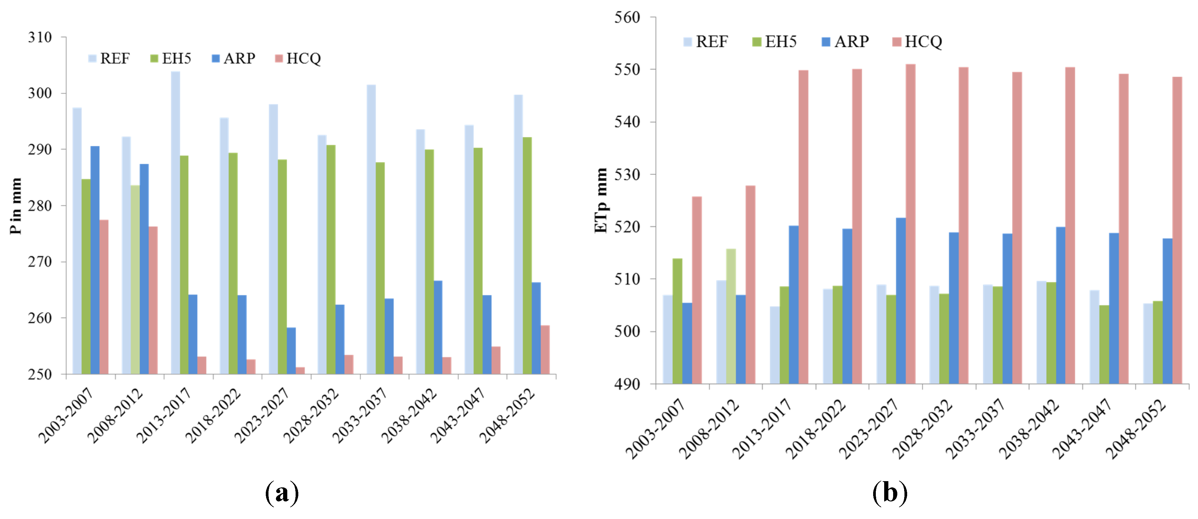
2.2.2. Applied Climate Projections in the WBalMo Model for the Study Area

A currently available installation of a WBalMo model on the Nuthe river basin served as the basis for our investigations at the case study area; this model was created by the German Federal Institute of Hydrology (BfG) and used for its own investigations of water availability for inland waterway transport. The BfG developed the stochastic input time series using the data from climate projections. First, we used the HYRAS data set, which represents a non-changing climate and features the daily values of meteorological variables over the period 1951–2006 with a spatial resolution of 5 km × 5 km [44]. The meteorological grid data was produced by regionalising station data from [43]. The stochastic time series, which is based on the HYRAS data set, is used as reference climate projection (REF). In addition, we used several climate projections based on scenario subset A1B of the Special Report on Emissions Scenarios (SRES) by the Intergovernmental Panel on Climate Change (IPCC); this scenario puts equal emphasis on all energy sources. From the 20 climate projections of the European Union’s ENSEMBLES research project [28], three climate projections were selected to cover the whole range of possible future climatic developments:
(1)
EH5r3_RE-ENS from the Max Planck Institute for Meteorology;
(2)
ARP-ALD51 from Météo-France, Centre National de Recherches Météorologiques; and
(3)
HCQ0-HRQ0 from the Hadley Centre for Climate Prediction and Research.
All three present a good reflection of the whole range of hydrological projections, particularly concerning low water, for the Lower Havel Waterway in the period 2021–2050 [45].
Climate projection EH5 estimates 2 to 14 mm less precipitation during the growing season from May to September compared to the REF (Figure 5). Next, precipitation and potential evapotranspiration of climate projection ARP for the period 2013–2017 are significantly lower than those of the REF. However, climate projection HCQ showed the largest deviation from the REF: the HCQ projects a decreasing precipitation of around 40 mm and an increasing potential evapotranspiration of 40–45 mm, which corresponds to a reduction of about 8% from the reference REF for the period 2013–2017.

2.2.3. Calculating Agricultural Irrigation Data to Expand the WBalMo Model for the Study Area

Some of the 43 farms in the study area operate with multiple water withdrawal sites in different sub-catchments. Therefore, each water withdrawal site in the sub-catchment where the withdrawal takes place was counted as one water user.
The basic assumption about irrigation water users is that every year over the entire model run time, they cultivate a fixed pattern of crops on the area of this irrigated land. The bases for deriving this crop distribution were (1) the irrigation acreage included in the legal permits for water withdrawal; (2) statistical surveys on irrigation used at district level under the 2010 agricultural census; and (3) the field-specific agricultural land use data from the Integrated Administration and Control System of the European Commission (IACS) [42].
Figure 5. (a) Average five-year precipitation and (b) potential evapotranspiration during the vegetation period (May to September) of the climate projections used in WBalMo.
Water 07 06351 g005
The total acreage of the several crops in the sub-catchments was determined from the field-specific IACS data [42]. While, IACS data does not provide information on irrigation, on the administrative district level (see Figure 2, black dotted lines) the acreage of irrigated crops are available. Therefore, the sub-catchments (see Figure 2, purple lines) were assigned to the administrative districts, which enables us to use the statistical surveys of (1) the acreage of a crop at district level ( A Distr C ) and (2) the proportion of the various crops that are irrigated ( A irr Distr C ) to calculate the share of crop acreage from the irrigated area in a district ( f irr Distr C ) as follows:
f i r r D i s t r C = A D i s t r C A i r r D i s t r C
Using the assignment of a sub-catchment ( ssc ) to a district, the irrigated acreage of a crop A irr  ssc C was calculated from the acreage in a sub-catchment A ssc F and the share of crop area from the irrigated acreage in a district:
A i r r   s s c C = A s s c F · f i r r D i s t r C
To accomplish this, the sub-catchment-specific crop distribution was assigned to each irrigation user affected.
The WBalMo model made available by the BfG was expanded to include the agricultural irrigation module, and all input data required was created for each irrigation water user. This way, all of his crops and the corresponding irrigated area are included. In addition, the monthly water withdrawal permits were assigned to each user. The parameters in Table 1, Table 2 and Table 3 and the control parameters for the start and stop of an irrigation event ( Θ Start u , c = 40% and Θ Stop u , c = 80%) were uniform for each user.
In our study site, most water users use groundwater for irrigation. Since WBalMo does not consider the groundwater reservoirs of a basin, it was necessary to implement virtual surface water reservoirs upstream of each node where irrigation users pump groundwater (see Figure 1). These virtual reservoirs simulate the behaviour of groundwater storage, and have a capacity equal to the amount of the user withdrawal permits. As with real groundwater withdrawal, they are recharged after each irrigation period.

2.3. Irrigation Management Scenario Analyses

The investigations were carried out using two irrigation management scenarios each using the same four climate projections listed above. The first scenario (SC_I) was based on present level of irrigation without any change to the irrigated acreage and crops. The second scenario (SC_II) was based on an increased irrigated acreage of each irrigation user without changing the crop composition. The irrigated acreage was assumed to double by 2018, based on the ongoing trend of increasing irrigation area. The amount of water withdrawal permits were doubled in the model analogous to the increasing area.
The WBalMo model of our study area simulates both irrigation management scenarios with all climate projections (1) REF as reference and (2) EH5, (3) ARP and (4) HCQ to take into account different possible forms of climate change. First, by comparing the results of climate projections 2–4 with those from the REF, it was possible to assess the range of impacts of climate change on the opportunities and impacts of irrigation in the SC_I irrigation management scenario.
Second, comparing the results of SC_II with those of SC_I delivered the additive impacts of increasing irrigated acreage on the irrigation water deficit, on the economic results of the irrigation, and finally on the water budget in the basin for each climate projection used.
As an outcome of the stochastic water management simulation, WBalMo generated frequency characteristics for five-year periods for water budget parameters, such as discharges. Additionally, the model calculated irrigation water demand and withdrawal, as well as additional crop yields and water supply costs, using its agricultural irrigation module and aggregating in the same manner for crop irrigation parameters.

3. Results

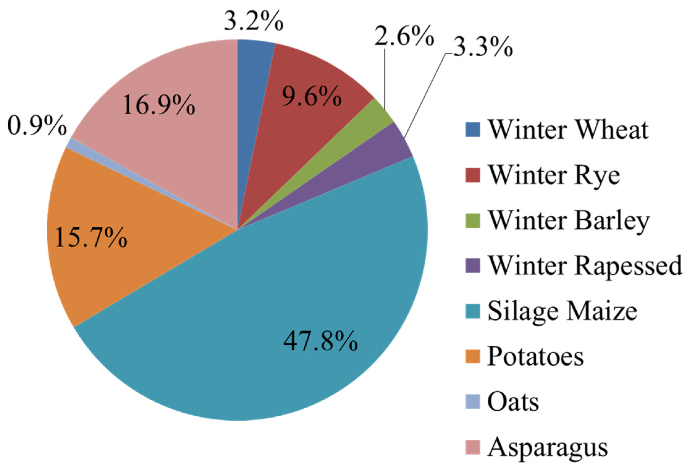
3.1. Irrigation Users and Irrigated Crops

The model simulated for 100 irrigation users, irrigating a total area of 6257 hectares (Figure 4). Thus, the irrigation area ratio of the whole study area is 3%. In total, about 12% of the arable land was irrigated. From a total of eight irrigated crops, maize was cultivated on 2990 irrigated hectares as the largest area, followed by asparagus and potatoes (Figure 6). The other five crops accounted for a total share of 20% of the irrigated area. These crops were cultivated on soils with very different water retention capacities. Most of the potatoes were produced in the southern part of the basin on sandy loess with an available water capacity from 109 to 133 mm. The rest of the soils were sand or loamy sand with an available water capacity from 48 to 67 mm. They were used to produce rye, rapeseed and maize. The sandy soils were used exclusively for asparagus.
Figure 6. Share of irrigated crops in the irrigated area in the study area.
Water 07 06351 g006

3.2. Testing the Module

In order to check the plausibility of the model results, the calculated irrigation demand amounts were compared with the actual amounts listed in the withdrawal permits of each user, employing the mean amounts of the irrigation water withdrawals calculated with the reference data (REF). All users remained under the permissible irrigation depth except User 8, who only exceeded it slightly (Figure 7). In all, 27 users (almost all of the Users 1–26 plus Users 70 and 91) cultivated potatoes on nearly half of their irrigation areas. Potatoes had the highest irrigation demand from June to August compared to the other crops (see below). In all, 78 users, almost all of the Users 27–79 and 87–100, used nearly 48%–65% of their irrigation area to produce silage maize. There were 57 users who irrigated asparagus on up to one-third of their overall irrigated area. Two of these users irrigated asparagus only. Due to the size of the enterprise and additional information these users were defined as specialised horticultural farms. Silage maize, asparagus and other cereal crops had a relatively low irrigation demand, so the distance between the calculated mean and permitted withdrawal is greater than that of the users growing mainly potatoes. In dry years, however, gaps between water demand and withdrawal are to be expected for those users who cultivate potatoes (Users 1–26) on nearly half of their irrigation area. In such cases water demands of up to 54 mm·year−1 in excess of the permitted values can be achieved.
Figure 7. Comparison of (red) irrigation permits and (blue) calculated average irrigation water demands (whiskers: 10th percentile) of each agricultural irrigation user of the simulation area in reference projection REF.
Water 07 06351 g007

3.3. Climate Impact (SC_I)

3.3.1. Future Development of the Irrigation Water Demand under Climate Change

Figure 8 shows a simulated future development of the average irrigation water demand for potatoes for all climate projections. This assumes that, relative to the current situation, neither irrigation intensity nor land management is altered in the area during the period under (SC_I). The irrigation water demand remains relatively stable over time within the individual climate projections considered. Only a slight decrease can be seen of about 0.4 mm·year−1 in reference projection REF and the ARP projection and less than 0.7 mm·year−1 in the other two projections. Irrigation demand of the reference projection was always lower than those of the climate projections. While the ARP projection was higher by about 5–9 mm·year−1 (and EH5 about 10–14 mm·year−1, respectively), for HCQ the difference to the reference projection was the greatest, with up to 30 mm·year−1.
Figure 8. Five-year irrigation demand of potatoes on average (bars: medians) and in dry years (whiskers: 10th percentile) for multiple climate projections.
Water 07 06351 g008
In dry years (10th percentile) the irrigation water demand of potatoes in climate projections fluctuated on average at around 210–215 mm·year−1, which was 37–40 mm·year−1 above the average in the reference projection. Compared to their average demands, the 10th percentile demands in the climate projections were always higher. In particular, the difference to the average demand was the smallest of all climate projections in the HCQ projection, at 4–9 mm·year−1.
Similar dynamics for the development of irrigation demand were also simulated for the other irrigated crops under all the climate projections given above. In the following, we limit the presentation of results to a consideration of the average percentiles for the overall irrigation parameters and for each of the crop types over the period 2018–2052.

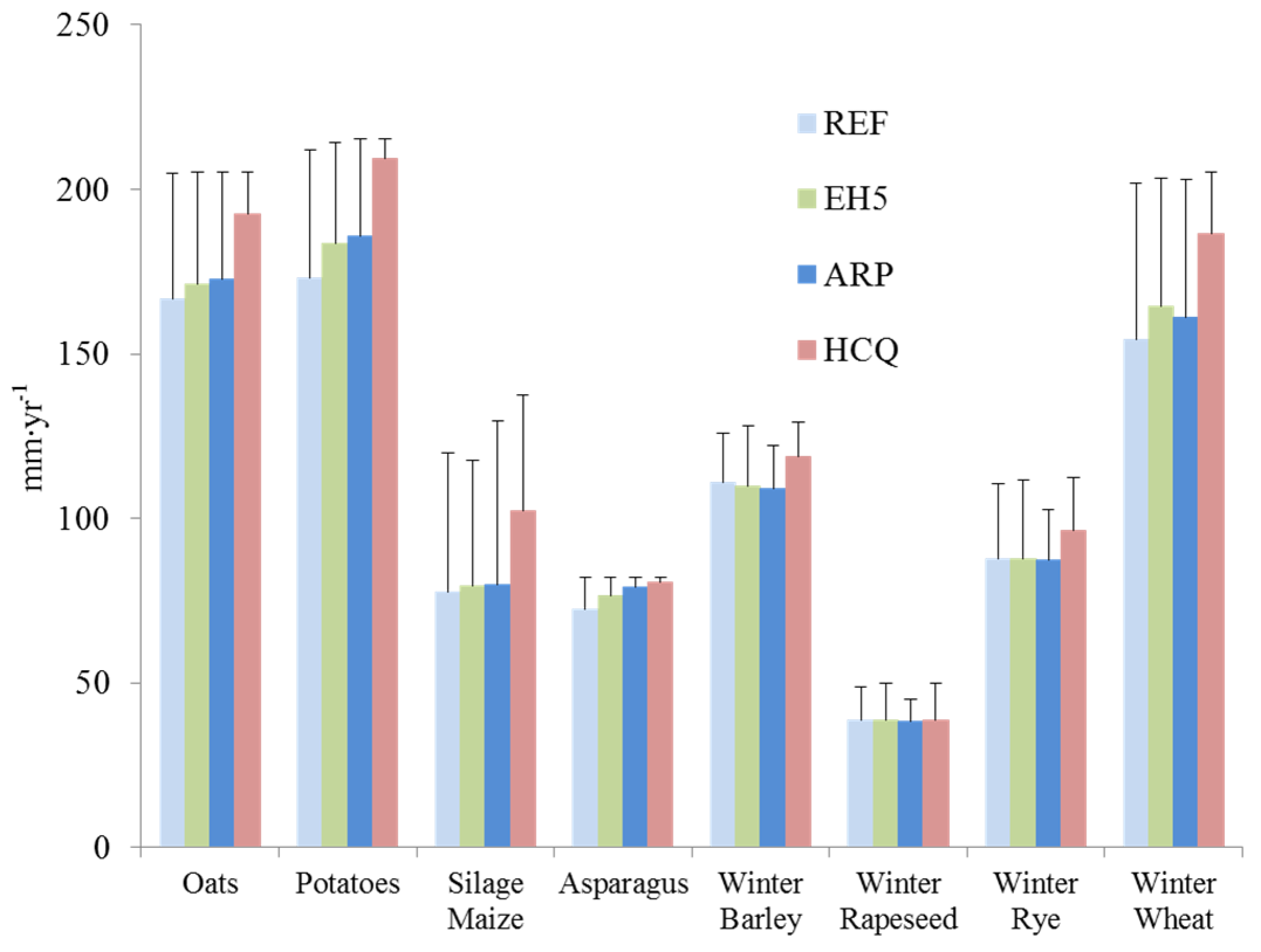
3.3.2. Crop Irrigation Demands under Conditions of Climate Change

Potatoes had the highest irrigation water demand of all crops and climate projections (Figure 9). The average demand of all irrigated potato areas was 183 mm·year−1 in the reference projection REF and 209 mm·year−1 with the HCQ projection. In dry years (10th percentile), an estimate of 211 mm·year−1 (216 mm·year−1 respectively) was even possible. Only a slightly lower demand was simulated for oats and wheat. The demand of barley and, with the HCQ projection, of maize also still exceeded 100 mm·year−1. However, the demand of all other crops was lower. At less than 50 mm·year−1, rapeseed had by far the lowest irrigation demand of all crops in each scenario. In this case, as well as for asparagus, the irrigation water demand increased the least in dry years compared to other crops.
Figure 9. Average crop irrigation demands for several climate projections in the period 2018–2052 (bar: medians, whiskers: 10th percentile).
Water 07 06351 g009

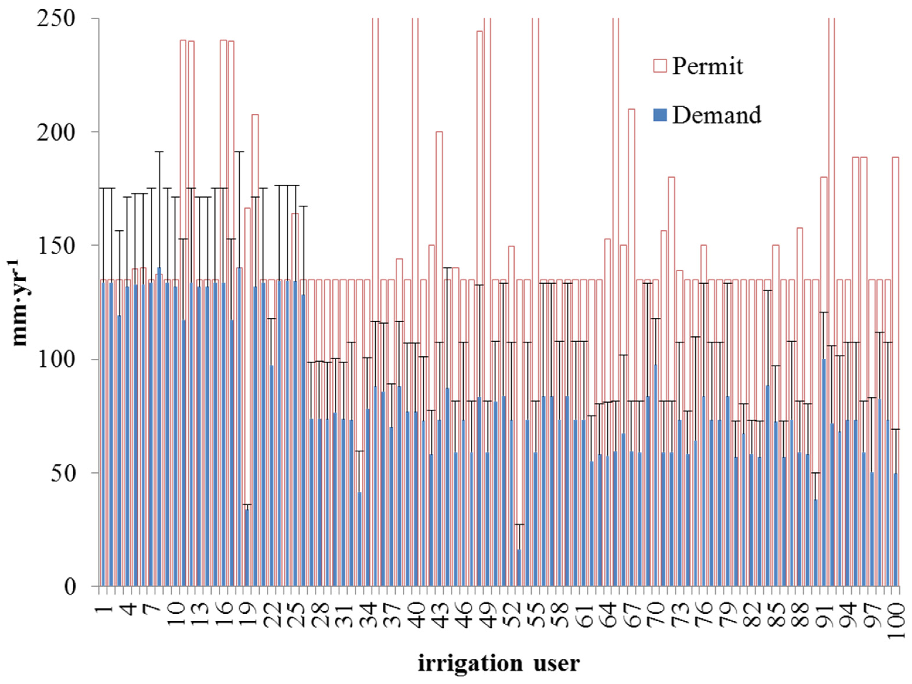
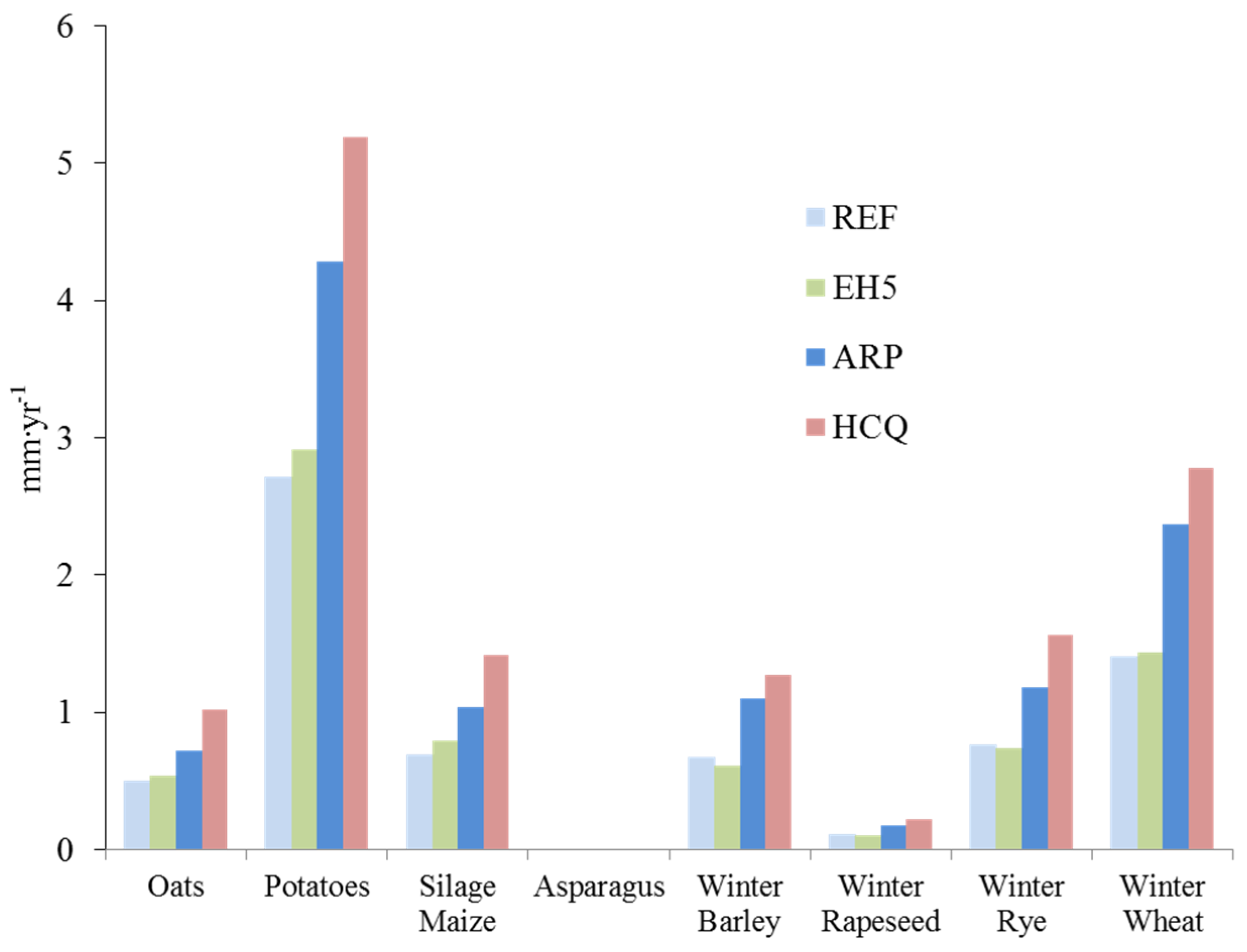
3.3.3. Gaps between Demand and Availability of Irrigation Water under Conditions of Climate Change

The model indicates that it is not possible to meet irrigation demand every year and for each crop in all climate projections. After all, very minor deficits resulting from the demand and availability of irrigation water were already yielded in the medians. The situation, however, was exacerbated in dry years (Figure 10). In those times, the water deficits for maize and potatoes were already 7.1 mm·year−1 and 4.5 mm·year−1 in the reference projection REF, respectively. The smallest deficits compared to the reference projection were yielded with the ARP projection. Other future effects greatly varied depending on the crop; for most cases, relatively small deficits appeared, always at a level less than 3 mm·year−1. However, in the case of maize, these deficits represented more than 6% of the average water demand, and even 9% in the reference projection. Most water deficits of other crops remained well below 3% of the average water demand.
Figure 10. Average irrigation water deficit for several climate projections in dry years (10th percentile) for the period 2018–2052.
Water 07 06351 g010

3.3.4. Agricultural Opportunities via Irrigation under Conditions of Climate Change

The irrigation applied to the crops led to additional yields based on the water productivity coefficient of each crop (Table 2). The highest additional yields for all projections were achieved for potatoes, followed by silage maize; this is based on their high productivity coefficients and the high priority assigned to these crops in the model (Figure 11). For all crops, additional yields were possible through irrigation although some crops encountered deficits (see Figure 9).
Figure 11. Average additional crop yields by irrigation for multiple climate projections in the period 2018–2052 (bar: median, whiskers: 10th percentile).
Water 07 06351 g011
The costs of irrigation reflected additional water withdrawals for each crop (Figure 12). The higher irrigation quantities in HCQ led to the highest irrigation costs for all crops compared to the other projections. Potatoes, oats and wheat generated the highest irrigation costs.
Figure 12. Average costs of irrigation for several crops and climate projections in the period 2018–2052 (bar: medians, whiskers: 10th percentile).
Water 07 06351 g012
Given their relatively high crop prices, asparagus and potatoes achieved the highest additional revenue compared to the other crops (Table 3). Here, too, the high irrigation quantities in HCQ led to higher additional revenue. For all crops, the additional revenue covered the additional costs of irrigation.
Table 3. Average additional revenue in the reference projection and their relative changes in the climate projections by irrigation for crops in the period 2018–2052.
CropREF (€·ha−1·year−1)EH5ARPHCQ
Oats3152%2%15%
Potatoes24817%4%17%
Silage maize2017%8%27%
Asparagus923311%6%16%
Winter barley1602%0%10%
Winter rapeseed1117%4%16%
Winter rye1573%−1%11%
Winter wheat4094%0%16%

3.3.5. Impacts of Agricultural Irrigation under Conditions of Climate Change

Based on climate projections and assuming that the irrigation intensity does not change in terms of either area or the management arrangement of irrigation water, changes in the stream flow are also to be expected. From May to September, the stream flow rates simulated at the reference projection in the study site were 87–246 L·s−1 (Table 4).
Table 4. Simulated average monthly stream flow rates at the basin catchment outlet in the reference projection (Q) and its projected changes due to climate change (ΔQ SC_I) and increased irrigation area (ΔQ SC_II) in the climate projections (time series 2018–2052).
MonthClimate Projection
REFEH5ARPHCQREFEH5ARPHCQ
Q (L s−1)ΔQ SC_I = SC_I − REFΔQ SC_II = Q SC_II − Q SC_I
May246−30%−49%−55%−1%−1%−1%−1%
June1486%32%−32%−2%−2%−2%−1%
July87−49%10%−62%−4%−3%−4%−2%
August106−64%13%−61%−3%−1%−2%−1%
September116−11%−11%−75%−3%−4%−1%−1%
However, the climate projections (SC_I) indicated the change in mean stream flows during the months with irrigation in detail (Table 4). As expected, the HCQ projection indicated the largest flow decrease (32%–75%). Projections for the EH5 projection were more moderate; a slight increase was even predicted in June, albeit a slight one. Only in the ARP projection could a moderate increase in the flows in all summer months be expected. In May and September, however, it followed the downward trend of the other two projections.

3.4. Area Impact (SC_II)

3.4.1. Impacts of Agricultural Irrigation under Conditions of Area Expansion

With climate change (SC_I), declining mean stream flow rates were already a threat in at least two projections. Doubling the irrigated agricultural area under irrigation management scenario SC_II would further reduce mean monthly stream flow rates (Table 4). This could be seen in each climate projection, albeit with very low relations from about 1% to 4%. The smallest declines were simulated with the HCQ projection because it already had the clearest declines as a result of climate change (SC_I). However, without climate change, the mean monthly stream flow rate was also reduced, if slightly less. Overall, these stream flow rate declines were much lower than those anticipated when induced solely by climate change.

3.4.2. Gaps between Demand and Availability of Irrigation Water Due to Area Expansion

As expected, the average yearly irrigation water deficit (Figure 13) rose due to the basically doubled water demand for almost all crops compared to scenario SC_I (Figure 10). However, these increases were relatively low and might be in the range of model uncertainty. Only in climate projections ARP and HCQ did the deficit of water for potato irrigation exceed 3 mm·year−1 and, in the latter, even 5 mm·year−1 which, however, was still less than 3% of the average irrigation water demand.
Figure 13. Changes in the average yearly irrigation water deficit through irrigation management scenario SC_II compared to climate projection SC_I for multiple climate projections of the period 2018–2052.
Water 07 06351 g013

3.4.3. Crop Yields with Irrigation under Conditions of Area Expansion

With a larger irrigated area, additional crop yields will of course rise in absolute terms. To compare these effects in all climate projections, area-specific additional crop yields are addressed below. This management scenario led to a relatively minor decline in average additional crop yields (Figure 14). Only for potatoes in the climate projections ARP and HCQO-HRQO was the decline between 2% and 3%, in line with increasing deficits (Figure 13). The declines in all other crops were not greater than 2% and might already be in the range of model uncertainty.
Figure 14. Change in average yearly additional crop yields by irrigation through irrigation management scenario SC_II to irrigation management scenario SC_I for multiple climate projections of the period 2018–2052.
Water 07 06351 g014

4. Discussion

4.1. Test und Interpretation of the Model

The irrigation module presented in this paper provided plausible results in terms of irrigation quantities, water deficits and economic variables considering water management practice in the basin. To prove this, among other things, the present mean irrigation water withdrawals were tested against the present permit for each irrigation user (Figure 3 and Figure 7). Note that when a crop making up a smaller proportion of the area had a higher water demand (e.g., Figure 9), this did not immediately affect a user’s irrigation water withdrawal (Figure 7). For medium irrigation amounts, the permitted withdrawal should be sufficient and no legal conflicts would occur, and this was true for all users. However, in years drier than the average, demand can be expected to exceed supply, in particular for users mainly growing potatoes. How this is handled in practice depends on the respective permit conditions. Our model cut off the water withdrawals if the permitted withdrawal was reached (see Figure 3).
The modelling of groundwater withdrawal for irrigation using virtual uncontrolled reservoirs led to a potentially unreliable evaluation of the reaction at low flows. Since the impacts in reality should in time be somewhat delayed and possibly spread a little wider, actual effects may have been overestimated. Nevertheless, the large difference between the effects of climate change and those of increased acreage of irrigation should remain unaffected.
The calculated irrigation water demand for single crops was somewhat similar to values found in other studies for the same region [46] (e.g., Figure 9), but with some significant differences due to differing assumptions on irrigation coefficients, different methodologies and climate trends. There can also be uncertainties with regard to climate change through the non-consideration of increasing water use efficiency due to an increase in CO2. We are aware that this might lead to an overestimation of future irrigation water demands and an underestimation of the achievable yields. Indeed, Kersebaum et al. [46] postulate an underestimation of the winter wheat yield of 11% for Germany when the CO2 effect is not factored in. However, for the purpose of our study, this effect can be neglected.
In order to consider the large uncertainties of climate change, three climate projections based of the scenario subset A1B of the Special Report on Emissions Scenarios (SRES) by the Intergovernmental Panel on Climate Change (IPCC) were selected which covered the range of all projections from drier (HCQ) to moister (EH5), around a medium projection (ARP). The impact of climate change was then assessed by comparing the reference climate projection (REF) without changes with the three change projections for the same time periods. All climate projections describe a lower precipitation and a higher evapotranspiration, with the exception of EH5 (Figure 5).
The impact of selected climate projections on the irrigation demand was relatively uniform over the seven five–year intervals. The very low temporal trend of the irrigation demand can be disregarded (Figure 8), as this corresponds to an increase in the irrigation demand over time of less than 3% (with the smallest amount as a basis). Thus, the focus within our study on aggregated values such as averages or percentiles of the time series from 2018 to 2052 appeared justifiable.
Furthermore, with regard to interpreting the compared results, e.g., for average crop water demands, it must be noted that such demands were the sum of all irrigation water users with this crop under the same climatic conditions. However, only users from a specific sub-catchment shared the same soil type areas and cropping patterns. Our module distributed the available irrigation water according to a crop ranking list (Table 2) for each user, such that crops with a lower priority might be irrigated less often than crops with a higher priority. Furthermore, the priorities between different water users (farms vs. non-agricultural water users) can change water availability in sub-catchments, leading to localised or temporary water deficits for certain users. Overall, the scenario-driven approach to handling water distribution between competing water users was sufficiently detailed. Moreover, the simulated competition of different crops may have reflected farmers’ behaviours more accurately than in most optimisation approaches, e.g., [47,48]. For our purposes, it can be used to describe the effects of climate change and an increasing irrigation area.

4.2. Opportunities

The agricultural irrigation in the study area was characterised by a large share of silage maize, mainly used as a renewable resource for biogas plants. Asparagus made up a relatively large part of the region as a field vegetable preferring light soils. Potatoes covered a slightly smaller share, with high demands in terms of reliable quality and quantity as a result of contract farming with manufacturers. However, with irrigation, the highest additional crop yields were achievable for potatoes and also for silage maize. Both had a high gross margin.
Schaldach et al. [49] underline the importance of socio-economic drivers for the increase in agricultural irrigation for Europe and its neighbouring regions. While our results showed a relatively high increase in crop irrigation water demand induced through the climate projections, it still depends on how farmers react to both climatic and economic changes. Irrigation can only be applied if price structures allow for its profitable application. Overall, recent trends in both climate and crop prices are leading to higher demand for irrigation water as well as a larger and more irrigated area.
Falloon and Betts [50] highlighted the uncertainty regarding climate impacts on European agriculture and water management. Adaptations to climate change not only lead to higher demand for irrigation water, but can also result in changes of crops, varieties or complete agricultural systems. Our results are therefore to be understood as the outcome of a conservative approach in adaptation to climate change, i.e., reacting only by adjusting the amount of irrigation. In the long run, other adaptation strategies might be more efficient and profitable.
Price variability was not considered in our study. Finger [51] has observed that if price volatility is high, water demand can be much lower as compared to a situation where farmers consider prices relatively fixed. Moreover, this effect has been proven in some parts of Germany by the high irrigation demand in contract farming (e.g., potatoes) where consistent quality is rewarded with higher prices and a price guarantee.
The results also show that the climate projections would have divergent effects on different crops. Changes in the rainfall pattern affect water availability and therefore crop-specific water deficits. If such changes in rainfall patterns become consistent, a change in the region’s crop shares can lead to more efficient water use.
Doubling the irrigation area naturally leads to an increase in total irrigation water demand. Since the share of the irrigated area compared with the total agricultural area is still rather low, a sufficient supply of irrigation water is generally available. However, this supply might not be available at all locations for dry years.

4.3. Impacts

In all climate projections, climate changes presented the largest impact on stream flow rates over the 2018–2052 time span. On the one hand, the irrigation demands should increase due to higher temperatures and drought stress during the cropping season depending on the crop type, generally up to 9% in the wetter projection and up to 17%–32% in the drier projection (HCQ) (Figure 9). On the other hand, the water supply could likewise decrease, due to higher temperatures in the region of the study area [52]. Given the rather small proportion of the area for irrigation, water is still sufficiently available in the basin under investigation. Of course, this may not necessarily be the case for some supply nodes and/or in dry years.
Nevertheless, two climate projections indicated a significant decrease in stream flow rates in May, July, August and September, ranging from a fall of 11% in the moister projection to 75% in the drier projection (Table 4). In a more moderate projection, this could be seen before and after the summer months, while during the summer months, there was even an increase in the stream flow rate. This means that a deep cut in the flow regime of the streams in the basin cannot be ruled out. Water users in the basin can expect constraints on water availability. Regardless of the climate change projections, the low flows in streams of the region of our study area were already low and there have been proposals to stabilise them [14,53]. Nevertheless, it is also clear that further warming will lead to intensified low flows in streams in the future [18].
The impact of an increased irrigation area on the flow regime was distinctly lower. Even doubling the current area only added 1%–4% to the stream flow reduction in the months with irrigation, in addition to reductions caused by climate change. In the drier projection the lowest reductions were yielded, as it already had the clearest declines due to climate change. This relatively low reduction in the stream flow rates compared to those caused by climate change is also due to the still small share of irrigated area in comparison with the total agricultural area. However, at 3–5 mm·year−1, only potatoes could be slightly affected by further deficits in irrigation water demand and availability (Figure 13). A marked decline in the yield increase due to irrigation is hardly something to be feared.
In the worst case, the effects of climate change and an increase in irrigated acreage could result in an aggravation of low flow in streams by up to 76% during 2018–2052. To avoid such situations, Wessolek and Asseng [4] suggest that the poor water retention soil sites in this region should already be managed extensively now, taking into account sufficient groundwater recharge, and that only the soils with better water retention properties be managed for sufficient agricultural production. Further possible measures were evaluated by [14]. Other proposals to address problems surrounding low flow could include the permit process. Most withdrawal permits have been granted for a limited time, in order to keep options open for future control (e.g., for climate change) in our case study region. In practice, a withdrawal permit could be cancelled or reduced. Further irrigation would no longer be possible, or the area being irrigated would have to shrink, or additional water-saving irrigation technologies would need to be implemented. Water consumption would decrease; however, the crop yield may also thus be lower. As a result, the profitability of the crop production would be affected as well.

5. Conclusions

The module developed can describe the processes of agricultural irrigation water use in a temporally and spatially differentiated way more effectively than conventional water management models based on WBalMo. In addition to water management, the module can also take into account economically driven irrigation decisions. Its application in the study area showed that climate changes will slightly affect the availability of irrigation water in the 2018–2052 period. However, in drier years, competition from other water uses, such as the drinking water supply, minimum ecological flows in streams or the conservation of wetlands, can create constraints on water availability. Nevertheless, the impact of climate change on the low flow situation in streams was much higher, meaning that a further expansion of irrigation calls for the careful monitoring of water availability to mitigate additional impacts on low flows. Furthermore, since the basic model is already in use by the water authorities, it can also be used to test the impact of issuing new permits or that of new water management policies.

Acknowledgments

This work was carried out with financial support from the Federal Office for Agriculture and Food (BLE) (project 2813HS007). We would like to thank Michael Kaltofen and Fabian Müller of the DHI-WASY company for the implementation of our model approach as a WBalMo module and Jens-Martin Hecker for providing the field-specific agricultural land use data. Our special thanks go to the German Federal Institute of Hydrology (BfG) for adding climate projections to the water management model for the study region and the State Office of Environment, Health and Consumer Protection of Brandenburg for allowing us to use it. We also thank our colleague Kurt-Christian Kersebaum for his valuable comments on the revised manuscript.

Author Contributions

Jörg Steidl developed the model approach and the concept of aggregating and evaluating the impacts of irrigation; he organised the use of existing WBalMo models with the relevant authorities, developed the databases for the model input data and the aggregation and evaluation of results, operated the model calculations and wrote the relevant sections. Johannes Schuler collected the information and data on agricultural irrigation management, developed the concept of aggregating and evaluating the opportunities of irrigation and wrote the relevant sections. Undine Schubert collected geodata and agricultural irrigation data, sought out other maps, constructed the geodatabase and connected it to the model input and result databases. Ottfried Dietrich worked on the development of the model module concept and the aggregation as well as evaluation of the model results. Peter Zander worked on developing the concept of evaluating of the opportunities of irrigation.

Conflicts of Interest

The authors declare that there is no conflict of interest.

References

  1. Riediger, J.; Breckling, B.; Nuske, R.S.; Schröder, W. Will climate change increase irrigation requirements in agriculture of Central Europe? A simulation study for Northern Germany. Environ. Sci. Eur. 2014, 26, 1–13. [Google Scholar] [CrossRef]
  2. Simon, M. Die landwirtschaftliche Bewässerung in Ostdeutschland seit 1949—Eine historische Analyse vor dem Hintergrund des Klimawandels; Summary Report No. 114; PIK-Praxis der Informationsverarbeitung und Kommunikation: Potsdam, Germany, 2009. [Google Scholar]
  3. Siebert, S.; Kummu, M.; Porkka, M.; Döll, P.; Ramankutty, N.; Scanlon, B.R. A global data set of the extent of irrigated land from 1900 to 2005. Hydrol. Earth Syst. Sci. 2015, 19, 1521–1545. [Google Scholar] [CrossRef]
  4. Wessolek, G.; Asseng, S. Trade-off between wheat yield and drainage under current and climate change conditions in northeast Germany. Eur. J. Agron. 2006, 24, 333–342. [Google Scholar] [CrossRef]
  5. Trnka, M.; Olesen, J.E.; Kersebaum, K.C.; SkjelvÅg, A.O.; Eltzinger, J.; Seguin, B.; Rötter, R.; Peltonen-Sainio, P.; Iglesias, A.; Orlandini, S.; et al. Agroclimatic conditions in Europe under climate change. Glob. Chang. Biol. 2011, 17, 2298–2318. [Google Scholar] [CrossRef] [Green Version]
  6. Holsten, A.; Vetter, T.; Vohland, K.; Krysanova, V. Impact of climate change on soil moisture dynamics in Brandenburg with a focus on nature conservation areas. Ecol. Model. 2009, 220, 2076–2087. [Google Scholar] [CrossRef]
  7. Nendel, C.; Kersebaum, K.C.; Mirschel, W.; Wenkel, K.O. Testing farm management options as climate change adaptation strategies using the MONICA model. Eur. J. Agron. 2014, 52, 47–56. [Google Scholar] [CrossRef]
  8. Bates, B.; Kundzewicz, Z.W.; Wu, S.; Palutikof, J. (Eds.) Climate Change and Water: Technical Paper VI; Intergovernmental Panel on Climate Change: Geneva, Switzerland, 2008; p. 210.
  9. Schindler, U.; Steidl, J.; Müller, L.; Eulenstein, F.; Jürgen, T. Drought risk to agricultural land in Northeast and Central Germany. J. Plant Nutr. Soil Sci. 2007, 170, 357–362. [Google Scholar] [CrossRef]
  10. Calzadilla, A.; Rehdanz, K.; Betts, R.; Falloon, P.; Wiltshire, A. Climate change impacts on global agriculture. Clim. Chang. 2013, 120, 357–374. [Google Scholar] [CrossRef]
  11. Mitchell, D. A note on rising food prices. In World Bank Policy Research Working Paper Series; World Bank: Washington, DC, USA, 2008; p. 22. [Google Scholar]
  12. Berbel, J.; Calatrava, J.; Garrido, A. Water pricing and irrigation: A review of the European experience. In Irrigation Water Pricing Policy: The Gap Between Theory and Practice; Centre for Agriculture and Biosciences International: Wallingford, UK; Cambridge, MA, USA, 2007; pp. 295–327. [Google Scholar]
  13. Gutzler, C.; Helming, K.; Balla, D.; Dannoowski, R.; Deumlich, D.; Glemnitz, M.; Knierim, A.; Mirschel, W.; Nendel, C.; Paul, C.; et al. Agricultural land use changes—A scenario-based sustainability impact assessment for Brandenburg, Germany. Ecol. Indic. 2015, 48, 505–517. [Google Scholar] [CrossRef]
  14. Thomas, B.; Steidl, J.; Dietrich, O.; Lischeid, G. Measures to sustain seasonal minimum runoff in small catchments in the mid-latitudes: A review. J. Hydrol. 2011, 408, 296–307. [Google Scholar] [CrossRef]
  15. Eheart, J.W.; Tornil, D.W. Low-flow frequency exacerbation by irrigation withdrawals in the agricultural midwest under various climate change scenarios. Water Resour. Res. 1999, 35, 2237–2246. [Google Scholar] [CrossRef]
  16. Jeppesen, E.; Kronvang, B.; Olesen, J.E.; Audet, J.; Sondergaard, M.; Hoffmann, C.C.; Andersen, H.E.; Lauridsen, T.L.; Liboriussen, L. Climate change effects on nitrogen loading from cultivated catchments in Europe: Implications for nitrogen retention, ecological state of lakes and adaptation. Hydrobiologia 2011, 663, 1–21. [Google Scholar] [CrossRef]
  17. Wegehenkel, M.; Kersebaum, K.-C. An assessment of the impact of climate change on evapotranspiration, groundwater recharge, and low-flow conditions in a mesoscale catchment in Northeast Germany. J. Plant Nutr. Soil Sci. 2009, 172, 737–744. [Google Scholar] [CrossRef]
  18. Thomas, B.; Lischeid, G.; Steidl, J.; Dietrich, O. Long term shift of low flows predictors in small lowland catchments of Northeast Germany. J. Hydrol. 2015, 521, 508–519. [Google Scholar] [CrossRef]
  19. Loucks, D.P.; van Beek, E.; Stedinger, J.R.; Dijkman, J.P.M.; Villars, M.T. Water Resources Systems Planning and Management: An Introduction to Methods, Models and Applications; UNESCO: Paris, France, 2005. [Google Scholar]
  20. Kaden, S.S.M.; Redetzky, M. Large-scale water management models as instruments for river catchment management. In Integrated Analysis of the Impacts of Global Change on Environment and Society in the Elbe; Basin, K.S., Wechsung, F., Behrendt, H., Klöcking, B., Eds.; Weißenseeverlag: Berlin, Germany, 2008; pp. 217–227. [Google Scholar]
  21. WBalMo 3.1–Interactive Simulation System for Planning and Management in River Basins; User’s Manual; WASY GmbH: Berlin, Germany, 2005.
  22. Koch, H.; Kaltofen, M.; Schramm, M. Adaptation strategies to global change for water resources management in the Spree river Catchment, Germany. Int. J. River Basin Manag. 2006, 4, 273–281. [Google Scholar] [CrossRef]
  23. Koch, H.; Kaltofen, M.; Grünewald, U.; Messner, F.; Karkuschke, M.; Zwirner, O.; Schramm, M. Scenarios of water resources management in the Lower Lusatian mining district, Germany. Ecol. Eng. 2005, 24, 49–57. [Google Scholar] [CrossRef]
  24. Dietrich, O.; Redetzky, M.; Schwarzel, K. Wetlands with controlled drainage and sub-irrigation systems—Modelling of the water balance. Hydrol. Process. 2007, 21, 1814–1828. [Google Scholar] [CrossRef]
  25. Dietrich, O.; Steidl, J.; Pavlik, D. The impact of global change on the water balance of large wetlands in the Elbe Lowland. Reg. Environ. Chang. 2012, 12, 701–713. [Google Scholar] [CrossRef]
  26. Grossmann, M.; Dietrich, O. Integrated Economic-Hydrologic Assessment of Water Management Options for Regulated Wetlands Under Conditions of Climate Change: A Case Study from the Spreewald (Germany). Water Resour. Manag. 2012, 26, 2081–2108. [Google Scholar] [CrossRef]
  27. Grossmann, M.; Dietrich, O. Social Benefits and Abatement Costs of Greenhouse Gas Emission Reductions from Restoring Drained Fen Wetlands: A Case Study from the Elbe River Basin (Germany). Irrig. Drain. 2012, 61, 691–704. [Google Scholar] [CrossRef]
  28. Van der Linden, P.; Mitchell, J.F.B. ENSEMBLES—Climate Change and its Impacts: Summary of Research and Results from the ENSEMBLES Project. 2009. Available online: http://ensembles-eu.metoffice.com/docs/Ensembles_final_report_Nov09.pdf (accessed on 6 November 2015).
  29. Kwon, H.-H.; Lall, U.; Khalil, A.F. Stochastic simulation model for nonstationary time series using an autoregressive wavelet decomposition: Applications to rainfall and temperature. Water Resour. Res. 2007, 43. [Google Scholar] [CrossRef]
  30. Brockwell, P.J.; Dahlhaus, R.; Trindade, A.A. Modified burg algorithms for multivariate subset autoregression. Stat. Sin. 2005, 15, 197–213. [Google Scholar]
  31. Efstratiadis, A.; Dialynas, Y.G.; Kozanis, S.; Koutsoyiannis, D. A multivariate stochastic model for the generation of synthetic time series at multiple time scales reproducing long-term persistence. Environ. Model. Softw. 2014, 62, 139–152. [Google Scholar] [CrossRef]
  32. Conradt, T.; Koch, H.; Hattermann, F.F.; Wechsung, F. Spatially differentiated management-revised discharge scenarios for an integrated analysis of multi-realisation climate and land use scenarios for the Elbe River basin. Reg. Environ. Chang. 2012, 12, 633–648. [Google Scholar] [CrossRef]
  33. Koch, H.; Voegele, S. Dynamic modelling of water demand, water availability and adaptation strategies for power plants to global change. Ecol. Econ. 2009, 68, 2031–2039. [Google Scholar] [CrossRef]
  34. Kaden, S.O.; Schramm, M.; Redetzky, M. ArcGRM: Interactive Simulation System for Water Resources Planning and Management in River Basins; Taylor and Francis Group: London, UK, 2004; pp. 185–192. [Google Scholar]
  35. Allen, R.G.; Pereira, L.S.; Raes, D.; Smith, M. Crop Evapotranspiration: Guidelines for Computing Crop Water Requirements; FAO Irrigation and Drainage Paper No. 56; Food and Agriculture Organization of the United Nations: Rome, Italy, 1998. [Google Scholar]
  36. ATV-DVWK. Verdunstung in Bezug zu Landnutzung, Bewuchs und Boden. Available online: http://www.dwa.de/dwa/shop/produkte.nsf/B161983F251AD1B2C125753C003466B9/$file/vorschau_atv_dvwk_m_504.pdf (accessed on 6 November 2015).
  37. DVWK. Ermittlung der Verdunstung von Land- und Wasserflächen; Wirtschafts- und Verl.-Ges. Gas und Wasser: Born, Germany, 1996. [Google Scholar]
  38. Mirschel, W.; Wieland, R.; Wenkel, K.-O.; Nendel, C.; Guddat, C. YIELDSTAT—A spatial yield model for agricultural crops. Eur. J. Agron. 2014, 52, 33–46. [Google Scholar] [CrossRef]
  39. Offermann, F.; Banse, M.; Ehrmann, M.; Gocht, A.; Gömann, H.; Haenel, H.-D.; Kleinhanß, W.; Kreins, P.; von Ledebur, O.; Osterburg, B.; et al. vTI-Baseline 2011–2021: Agrarökonomische Projektionen für Deutschland—Sonderheft 355; Bundesforschungsinstitut für Ländliche Räume, Wald und Fischerei (vTI): Braunschweig, Germany, 2012. [Google Scholar]
  40. Kuratorium für Technik und Bauwesen in der Landwirtschaft (KTBL). Feldbewässerung: Betriebs- und arbeitswirtschaftliche Kalkulationen; KTBL: Darmstadt, Germany, 2013. [Google Scholar]
  41. Statistisches Bundesamt. Land- und Forstwirtschaft, Fischerei Bodenbearbeitung, Bewässerung, Landschaftselemente—Erhebung über landwirtschaftliche Produktionsmethoden (ELPM); Statistisches Bundesamt: Wiesbaden, Germany, 2011. [Google Scholar]
  42. European Commission. Integrated Administration and Control System (IACS). Available online: http://ec.europa.eu/agriculture/direct-support/iacs/index_en.htm (accessed on 19 May 2015).
  43. German Meteorological Service. Available online: http://www.dwd.de/DE/Home/home_node.html (accessed on 6 November 2015).
  44. Rauthe, M.; Heiko, S.; Ulf, R.; Alex, M.; Annegret, G. A Central European precipitation climatology—Part I: Generation and validation of a high-resolution gridded daily data set (HYRAS). Meteorol. Z. 2013, 22, 235–256. [Google Scholar] [CrossRef]
  45. Ebner von Eschenbach, A.D.; Hohenrainer, J.; Kaltofen, M.; Müller, F.; Schramm, M. Wasserwirtschaftliche Verhältnisse des Projektes 17 für den Bereich des WNA Berlin; Bundesanstalt für Gewässerkunde: Koblenz, Germany, 2013; p. 210. [Google Scholar]
  46. Kersebaum, K.C.; Nendel, C. Site-specific impacts of climate change on wheat production across regions of Germany using different CO2 response functions. Eur. J. Agron. 2014, 52, 22–32. [Google Scholar] [CrossRef]
  47. Bazzani, G.M.; di Pasquale, S.; Gallerani, V.; Morganti, S.; Raggi, M.; Viaggi, D. The sustainability of irrigated agricultural systems under the Water Framework Directive: First results. Environ. Model. Softw. 2005, 20, 165–175. [Google Scholar] [CrossRef]
  48. Rosegrant, M.W.; Ringler, C.; McKinney, D.C.; Keller, A.; Donoso, G. Integrated economic-hydrologic water modeling at the basin scale: The Maipo river basin. Agric. Econ. 2000, 24, 33–46. [Google Scholar]
  49. Schaldach, R.; Koch, J.; der Beek, T.A.; Kynast, E.; Flörke, M. Current and future irrigation water requirements in pan-Europe: An integrated analysis of socio-economic and climate scenarios. Glob. Planet. Chang. 2012, 94–95, 33–45. [Google Scholar] [CrossRef]
  50. Falloon, P.; Betts, R. Climate impacts on European agriculture and water management in the context of adaptation and mitigation-The importance of an integrated approach. Sci. Total Environ. 2010, 408, 5667–5687. [Google Scholar] [CrossRef] [PubMed]
  51. Finger, R. Modeling the sensitivity of agricultural water use to price variability and climate change-An application to Swiss maize production. Agric. Water Manag. 2012, 109, 135–143. [Google Scholar] [CrossRef]
  52. Roers, M.; Wechsung, F. Reassessing the Climate Impact on the Water Balance of the Elbe River Basin. Hydrol. Wasserbewirtsch. 2015, 59, 109–119. [Google Scholar]
  53. Thomas, B.; Lischeid, G.; Steidl, J.; Dannowski, R. Regional catchment classification with respect to low flow risk in a Pleistocene landscape. J. Hydrol. 2012, 475, 392–402. [Google Scholar] [CrossRef]

