1. Introduction
Over the past years, the number of electric vehicles (EVs) has rapidly increased in the Netherlands. The total number of Dutch electric passenger cars was about 143,000 by the end of December 2018 [
1], which is 1.7% of the Dutch passenger car stock. Of these EVs, 31.5% were battery electric vehicles (BEVs) and 68.4% plug-in hybrid electric vehicles (PHEVs) [
1]. The Dutch government aims at 50% of the new passenger cars sold being equipped with an electrical drive train in 2025, and 100% of all new passenger cars sold being zero-emission in 2030 [
1]. The increase in number of EVs goes hand in hand with an increase in the number of EV charging stations. By the end of December 2018, there were 35,894 public and semi-public charging points in the Netherlands, and about 100,000 private charging points [
1].
Previous studies have shown that, in residential areas, the EV demand peaks are likely to coincide with household demand peaks in the case of uncontrolled charging [
2,
3,
4,
5]. Uncontrolled charging means that EVs start charging at full power as soon as they are plugged in to a charging station, continuing until the battery is fully charged. Currently, this is the common way of charging in the Netherlands. Considering that by far the largest share of charging stations (99.4%) is currently connected to low-voltage (LV) networks [
6], uncontrolled charging is expected to cause grid congestion for increased EV fleet sizes [
5]. Smart charging is the redistribution of the charging demand over the period during which the EV is connected to the charging station. Apart from avoiding grid congestion caused by EV demand, smart charging can serve multiple other goals, for example, to provide ancillary services, to minimize charging costs, or to maximize the utilization of local renewable energy sources [
5,
7,
8,
9,
10,
11,
12].
One of the requirements for smart charging is the availability of sufficient EV demand flexibility. We define a transaction as one charging session with connection duration
including the entire process between connecting and disconnecting the EV charging cable to/from the charging point. Then, the maximum available flexibility during a transaction is determined by the difference between the connection duration (
) and the charging duration (
), with
being the period needed to charge the required energy (
Ereq) into the EV battery. In previous studies on smart charging, the maximum available EV demand flexibility was often assessed in a simplified way, not investigating the diversity in connection durations and charging durations for the different transactions. Lopes et al. [
11] used three types of EVs, with charging powers of 1.5, 3, and 6 kW, respectively, and an average value of 4 h for
. The study assumed that all existing vehicles plugged in at 21:00 in the evening. Clement-Nyns et al. [
12] divided the day into different time slots and assumed that all EVs had a maximum charging power of 4 kW. The EVs plugged in during a certain time slot and had to be fully charged by the end of the time slot, thereby underestimating the flexibility of EV demand, as in reality, the connection durations are expected to exceed the durations of the time slots used. Claessen et al. [
9] used a normal distribution of charging start and end times around a fixed mean, a maximum power flow of 3.7 kW, and discrete values for
Ereq per transaction (3, 6, or 12 kWh). Wu et al. [
7] used a plug-in time between 07:00 and 08:00 and a plug-out time between 18:00 and 19:00, the (dis)charging power was flexible between −10 and 10 kW, and
Ereq was assumed to be 12 kWh for each transaction. Jian et al. [
13] used a chi-squared distribution for arrival times and a normal distribution for the simulation of
, with a fixed mean of 10 h and a fixed standard deviation of 3 h, and a maximum charging power of 4 kW for all EVs. In the study by Van der Kam & Van Sark, a uniform distribution between 3 and 6 h was used for trip durations, and it was assumed that the EV was always connected when it was not on a trip, thereby overestimating the available flexibility [
8]. The maximum charging power was set at 6.6 kW or 22 kW in that study, depending of the type of EV that was simulated. Scharrenberg et al. [
14] used hourly frequency distributions of arrival and departure times from the Dutch national mobility study [
15] for defining the availability of EVs for smart charging. This is more realistic than using predefined distributions, yet the study did not consider connection durations of individual transactions nor the diversity of charging durations for different transactions. Further, a charging power of 3.7 kW was used for all EVs. Liu et al. [
16] used National Travel Surveys in the Nordic region to assess the availability of EVs for smart charging, but did not link this availability with charging durations. So far, only a few studies have been found that assessed the available EV demand flexibility by combining
and
. By taking into account the plug-in time (
) as well, the changes of available flexibility over time can be investigated. A study by D’Hulst et al. (2015) investigates time-dependent flexibility of several appliances, among which are EVs. The EV flexibility was based on a pilot in which seven EVs were monitored over a period of 10 weeks [
17]. The charging power of the EVs in the study was limited to 2.3 kW. To achieve a realistic assessment of the maximum potential flexibility of EV demand and the time dependency of the available flexibility, it is necessary to investigate the differences between
and
for a large number of transactions. The earliest study found in which this was done was published in 2017 and examines a Dutch and a Flamish dataset [
18]. The authors present a time-varying response potential in kW for different charging locations. A more recent study by Flammini et al. provides an extensive statistical analysis of EV behavior based on Dutch charging station data, including idle times [
19]. However, the authors give no clear results on how idle time, and thus the flexibility, varies over the time of the day. Another recent study analysed one year of Dutch present-day public charging station data, including the flexibility and its time-dependency [
20].
The purpose of this study is to analyse the maximum available flexibility of EV demand in a residential area, including the time-dependency of this flexibility, and to propose a method for the stochastic simulation of EV demand including detailed flexibility constraints. The results enable making accurate estimations of the maximum value of different smart charging schemes in residential areas, for example, in terms of reduced charging costs, reduced impacts on the low voltage network, and increased self-consumption of local photovoltaic (PV) generated electricity. In this study, an EV user participation rate of 100% and perfect forecast is assumed. In reality, perfect forecast is of course not feasible. However, in the pilot considered in this study, a certain amount of information on the flexibility constraints is available beforehand—the EV users that take part in the smart charging system communicate their estimated departure time and amount of energy needed to an aggregator when they connect their EV to the charging station. Besides, the aggregator is able to forecast future charging behavior based on historical data. The real-time user data in combination with the forecasted EV charging behavior enables the aggregator to plan the charging schedule in advance, taking into account the flexibility constraints. The charging stations in the pilot are owned and controlled by one company, but are accessible to everyone. Therefore, these charging stations are referred to as public charging stations in this study.
Most studies mentioned above use one value for charging power for all EVs. However, the available flexibility depends on
, which in turn depends on the charging power. Charging power is influenced by several factors such as outside temperature, battery state-of-charge (SoC), and battery age [
21,
22,
23]. Therefore, variations in charging power between different EVs and different transactions are investigated in this study as well.
Further, the paper proposes a method for simulating charging behavior of future EV fleet sizes, to investigate the future flexibility of EV demand. In previous studies, Markov Chain Monte Carlo has been used to simulate EV behavior [
24,
25]. In the present study, this method was not used because mobility patterns in general do not fulfill the Markov property as they are not memoryless—the time of departure from a location is dependent from the time of arrival at that location, which is in turn influenced by the departure time from the previous location [
26]. Also, in reality, the variables
,
, and
are statistically dependent [
24,
27], which is not reflected in Markov Chain Monte Carlo analysis. For these reasons, in this study, a stochastic Monte Carlo simulation was used in which the interdependencies between
and
, between
and
, and between
and
are respected. This simulation was used to examine the availability of EV demand flexibility and its variation over time for future EV fleets. Three different methods for simulating the charging power were compared. The first one uses a fixed charging power based on the maximum power that the charging point can deliver or the maximum power that the EV is able to charge with. The other two methods both use charging power values that vary per simulated transaction. The values for charging power are randomly selected from the transaction-specific maximum and average values from the measured charging power profiles.
The method for investigating EV demand flexibility was used to analyse available flexibility for a case study in a residential area in the city of Utrecht, the Netherlands. In this project, 21 charging stations were logged over one year. The outcomes from the flexibility analysis are used as input for the simulation of charging behavior of future EV fleets and the time-dependent flexibility of the resulting EV demand. The case study is performed to illustrate the proposed method for assessing EV demand flexibility.
The paper is structured as follows. In
Section 2, the method for the analysis of EV demand flexibility and the method for the simulation of future EV demand flexibility are described. In
Section 3, the case study is described. Then, in
Section 4, the results are presented. The methods and results are discussed in
Section 5. In
Section 6, a conclusion and pointers for future work are given.
2. Methods
In this section, first the data analysis is described.
Section 2.1 describes the analysis of the time-dependent flexibility of EV demand, and
Section 2.2 explains the division of the EVs into different categories. Then, we explain the method used for the EV simulation. In
Section 2.3, the method for setting up the simulated EV fleet size scenarios is given.
Section 2.4 describes the data preparation for the simulation, and in
Section 2.5, the simulation steps are explained. All data analyses and the simulations have been performed using Python 3.7 on Spyder 3.3.1.
The minimum data requirements to carry out the proposed flexibility assessment are, for each EV transaction i, as follows:
: the plug-in time for transaction i.
: the plug-out time for transaction i.
: power charged at each time t during transaction i, with a sufficiently high time resolution ( ≤ 15 min). In this study, this data is referred to as the ‘measured charging profile’.
Possibly also [kWh], which is the total charged energy during each transaction. However, this metric can also be derived from if is sufficiently small.
A unique anonymous identity for each EV j that occurs in the dataset. For each transaction i in the dataset, the identity of the charging EV j must be known.
2.1. Analysis of Time-Dependent Flexibility of EV Demand
The connection duration for transaction
i (
is the period of time during which an EV charging cable is connected to the charging point, which is calculated using Equation (1).
[h] can be derived by counting the number of non-zero values for
during transaction
i, as expressed in Equation (2), in which
is the timestep of the charging power data. For uncontrolled transactions, there will be a continuous series of non-zero values starting at
for each transaction
i.The difference between
[h] and
[h] defines the available flexibility, in hours, during transaction
i, and is referred to as
. This is expressed in Equation (3).
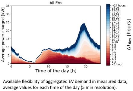
By aggregating the values of
for all transactions
i, the aggregated EV demand, defined as
[kW], is derived. Using Equation (3), for each transaction
i, it is calculated for how many hours the demand could be delayed. On the basis of this information, the available flexibility of aggregated EV demand
at each moment in time is calculated. The definitions of
,
, and
are illustrated in
Figure 1.
In this study, the measured charging power profiles of each separate transaction
i are analysed. For each measured charging power profile, three approximated constant charging power profiles are defined. An example of a measured charging power profile of a BEV and the corresponding three different constant charging power profiles is illustrated in
Figure 1. For all four profiles,
is kept the same, meaning that the area under the measured charging power profile and all three constant charging power profiles is equal. For the green profile shown in
Figure 1, a fixed charging power (
[kW]) is used.
is chosen depending on the type of EV or the type of charging station. In the example in
Figure 1, it is 22 kW, which is the maximum power output of a 3 × 32 A AC 230 V charging point. The second and third constant charging power profiles are based on the maximum (blue profile in
Figure 1) and average charging power (red profile in
Figure 1) during
, respectively. As the average and maximum charging power during
differ for each transaction
i, these charging powers are referred to as ‘transaction-specific’. Below, the characteristics of the three constant charging power profiles based on the three different values for charging power are described:
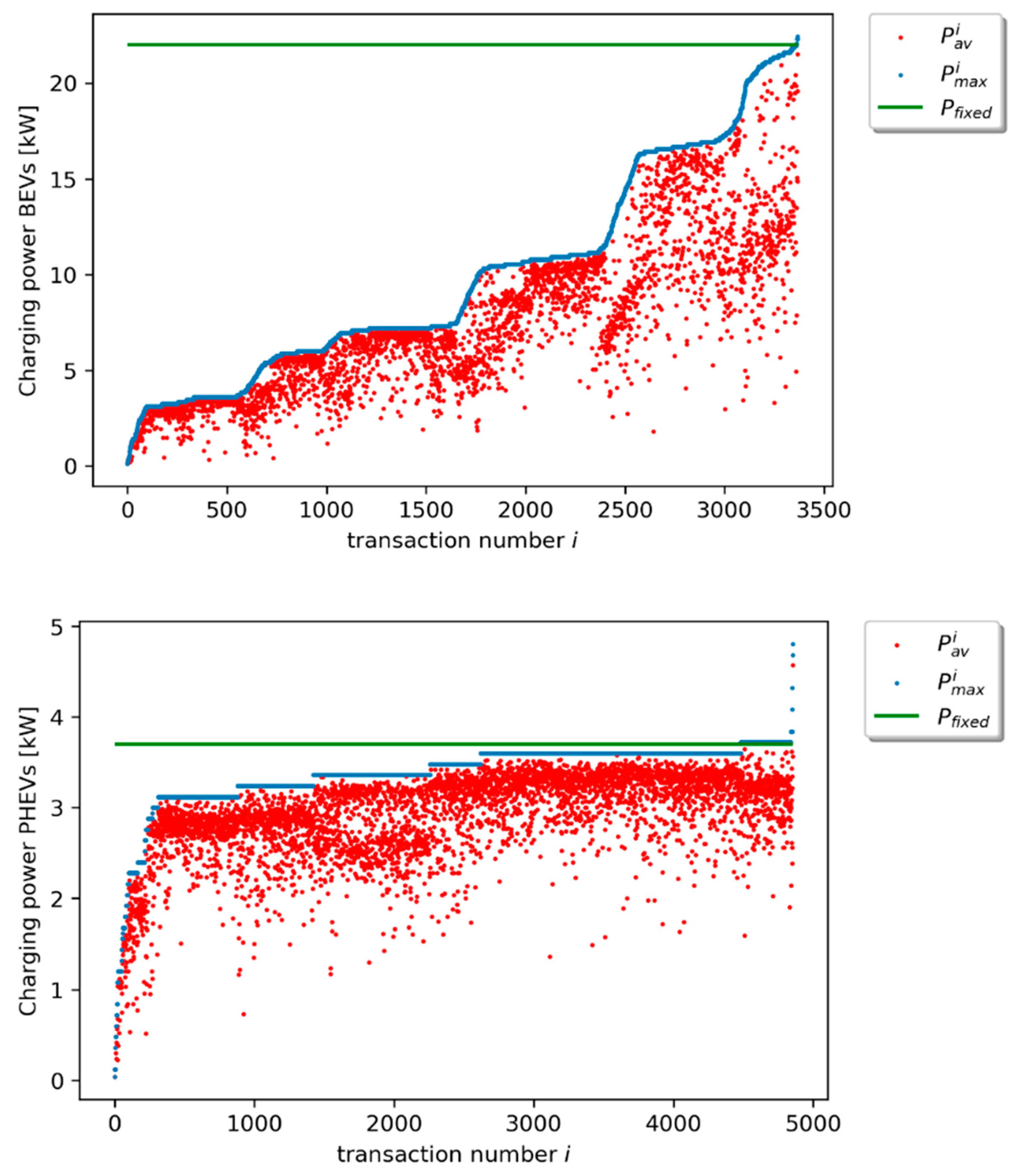
Fixed constant charging power,
[kW], which can be chosen depending on the type of car or the type of charging station. The charging duration for this fixed constant charging power profile is
, which is calculated using Equation (4).
Transaction-specific maximum constant charging power [kW], is the maximum value of charging power
that occurs during transaction
i. The charging duration
is calculated using Equation (5).
Transaction-specific average constant charging power,
[kW], is the average power of transaction
i, which is calculated using Equation (6).
is equal to the measured charging duration
.
2.2. EV Categories
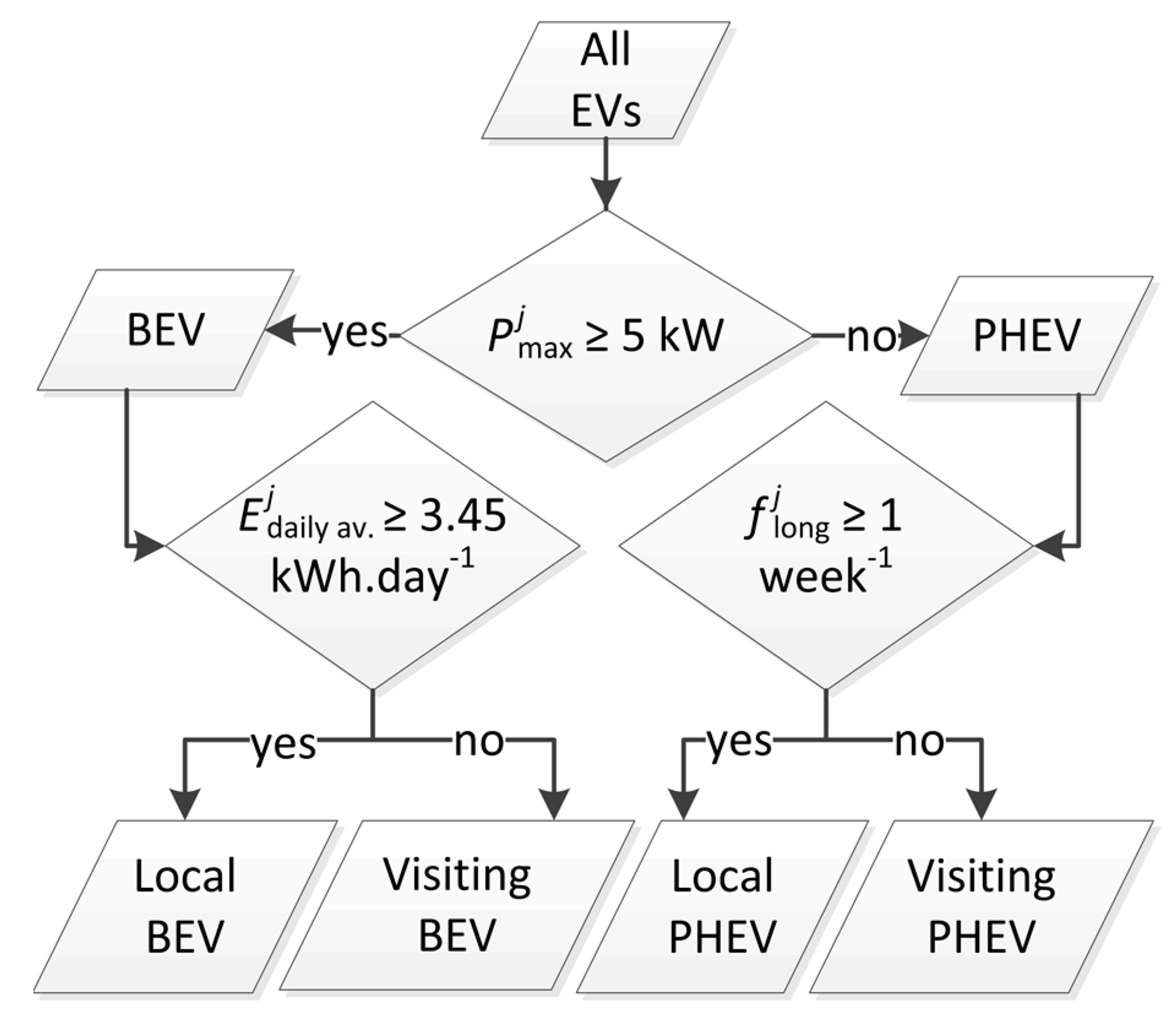
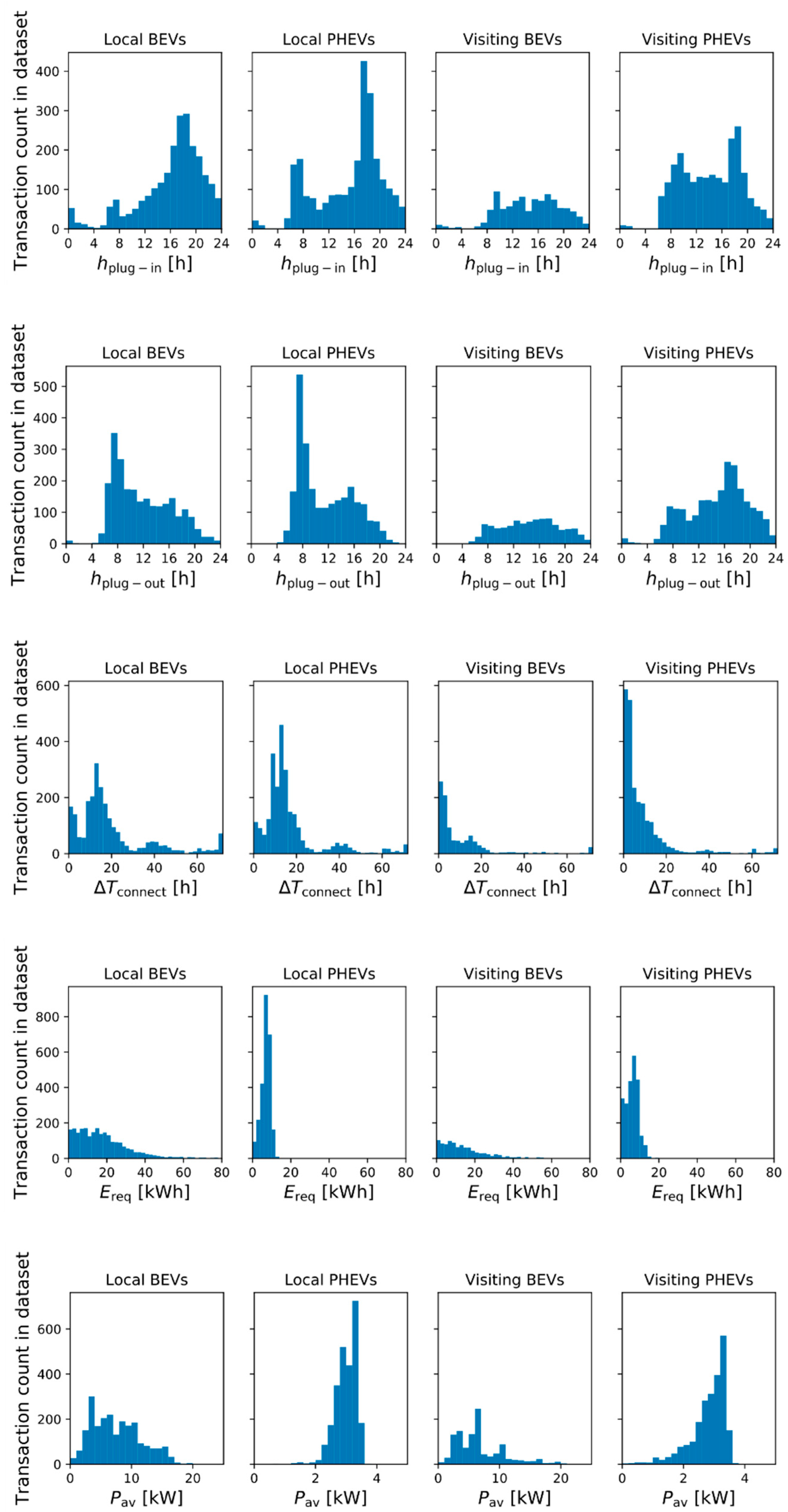
To obtain more insight into the charging behavior of the EVs and to provide a basis for the simulation of future scenarios, the EVs are categorized, resulting in four different categories. It is usually not possible to link the identity of the users to the EV identities (IDs) because of privacy reasons. Therefore, the categorization is based on a unique anonymous identity for each EV j that occurs in the measured dataset, , where is the number of unique EV IDs in the measured dataset. For each transaction i, the identity of the charging EV j is known.
First, the EV IDs are split into two main categories, namely BEVs and PHEVs. This is done because charging behavior is different between these types of EVs and because the share of BEVs in the total EV fleet is expected to grow in the future [
28]. The division between BEVs and PHEVs is based on the maximum charging power at which each EV
j charged during the measurement period (
[kW]). For the top five best sold PHEVs in the Netherlands, which cover 66% of the total number of Dutch PHEVs, the maximum charging power is 3.7 kW [
1,
29]. Therefore, an EV is considered a BEV if
≥ 5 kW and a PHEV if
< 5 kW. Further, as EVs owned by people living in the area were expected to charge more frequently and have longer connection times, a division between local and visiting EVs is made. A BEV is considered to be local (i.e., owned by residents) if its average daily charging demand (
[kWh·EV
−1·day
−1]), averaged over the year, exceeds a certain threshold. The demarcation is set at 3.45 kWh·day
−1, which is 50% of the average daily energy demand of a Dutch electric passenger car, based on an average daily distance of 34.6 km [
30,
31] and a driving efficiency of 5 km·kWh
−1 [
32]. This assumption was found to yield meaningful results (see
Section 4.1). For PHEVs,
is less informative as the share of electricity demand in their total energy demand is unknown. Therefore, for PHEVs, the frequency of long transactions (
[week
−1]) is used as a decision parameter, in which a long transaction was defined as a transaction with a connection duration of over 6 h. The division of EVs is illustrated in
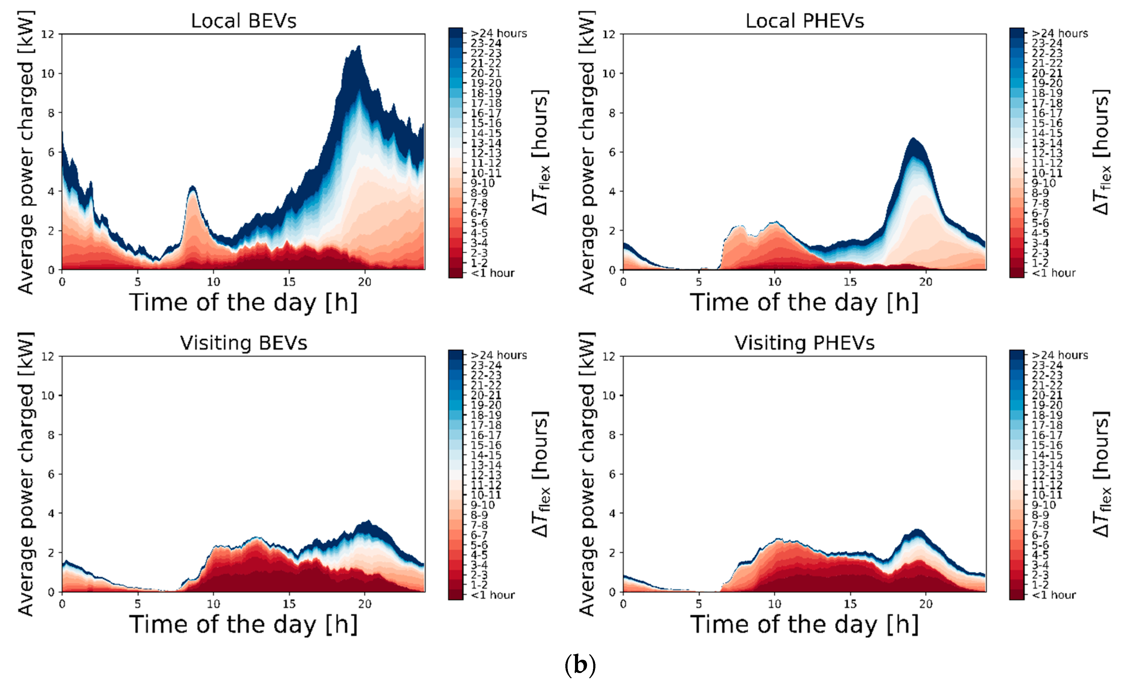
Figure 2. Using this division, the available flexibility can also be expressed per EV category by selecting only transactions by EVs from a certain category.
2.3. Scenarios EV Fleet Size
In this section, the method for deriving the scenarios for future EV fleets charging in the simulated area is described. For this study, three scenarios are set up, namely, ‘Present-day’, ‘Medium’, and ‘High’.
To derive the number of unique EVs charging in the ‘Present-day’ scenario, the number of unique EVs charging in the measured data is multiplied by the ratio of the number of charging points in the simulated area to the number of charging points in the total area in which the charging data were measured. This is expressed in Equation (7), assuming that the EV density in the simulated area is equal to that in the total area. This step is only needed if the simulated area is smaller than the total area for which the charging data were collected.
In Equation (7), is the present-day number of simulated unique EV IDs in a certain category associated with the simulated area, is the number of unique EV IDs in that category occurring in the total measured dataset, is the number of charging stations in the simulated area, and is the total number of charging stations in the dataset. The outcome is rounded to the nearest integer. Note that the number of charging stations in the area is only used to define ; in the simulation, it is assumed that the number of charging stations is perfectly demand driven, meaning that the number of simultaneously charging EVs is left unconstrained.
Further, the following assumptions are made:
The car possession rate (CPR [HH−1]), which is the number of passenger cars per household (both EV and non-electric), is the same in all scenarios.
In the ‘High’ scenario, all passenger cars will be BEVs, based on the Dutch governmental target of 100% of the passenger cars sold in 2030 being emission free [
1].
In the ‘High’ scenario, the maximum number of unique visiting BEVs per month is limited to 50 times the current number of charging stations in the area.
The difference in number of EVs between the ‘Current’ and the ‘Medium’ scenario is half the difference between the ‘Current’ and the ‘High’ scenario for each EV category.
The lifetime (LT) of an EV is assumed to be 15 years [
33].
Applying assumptions 1, 2, and 5, the number of local BEVs in the ‘High’ scenario is calculated using Equation (8).
In Equation (8),
is the number of simulated local BEVs in the ‘High’ scenario,
is the number of households,
[HH
−1] is the car possession rate, LT [year] is the lifetime of an EV, and
is the number of days in the measured dataset. By combining this with the current number of EVs occurring in the dataset, the size of the different EV categories can be derived for each scenario. The scenarios are not associated with specific years, as it is uncertain when a 100% EV market share will be reached in the Netherlands [
34].
2.4. Simulation: Preparation Input Data
In this section, the preparation of the input data for the EV simulation is explained. The aim of the simulation is to investigate the maximum available flexibility of future EV fleet sizes using available measured charging station data. Because the simulation of the maximum available flexibility is desired, EV demand peaks and flexibility are simulated assuming uncontrolled charging.
As explained in
Section 2.2, four different EV categories are distinguished. These categories have to be considered in the simulation because the composition of the EV fleet is expected to change in the future, in other words, the different categories’ shares of the total fleet size will not remain constant. Further, the energy charged and the connection duration of transactions probably varies during the course of a day. For example, the probability of high values for
and
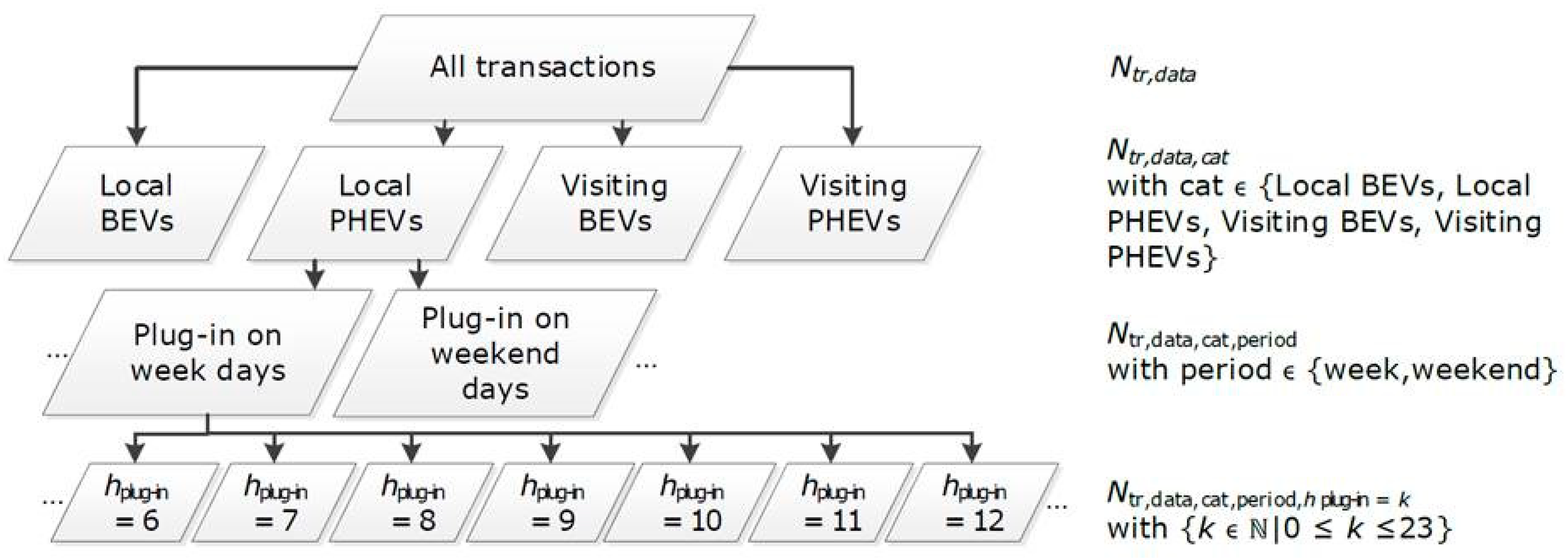
might be higher for a transaction starting in the evening than for one starting in the morning. The time-dependency of these parameters has to be accounted for in the simulation as it defines the intra-daily changes of EV demand impact and flexibility. Lastly, the charging behavior also differs between week and weekend days.
For these reasons, the measured transactions are split into different subsets. The first division is made based on the EV categories, resulting in four sets with size
, as depicted in
Figure 3. Then, these sets are divided into transactions during the week and transactions during the weekends. Each of these eight sets has size
(see
Figure 3). To take into account the variation of transaction properties with the time of the day, each of the 8 sets with size
is further split into 24 sets based on starting hour of the transaction, resulting in 8 groups of 24 sets, each containing a number of transactions equal to
(the bottom row of
Figure 3). The distributions of
and
in each of these sets were tested on similarity with the distributions in the other 23 sets from the same group, that is,
using a non-parametric two-sample Kolmogorov–Smirnov test [
35,
36]. The set with size
is considered similar to another set if the frequency distributions of both
and
showed no significant (
p ≤ 0.05) differences between the two compared sets. This way, each set with size
is associated with similar sets in the same group.
2.5. Simulation Steps
For each of the simulated EVs m in a certain EV category, the following steps are taken during the simulation:
From the available data, for each EV
j in the dataset the number of transactions is normalized to the simulation period using Equation (9).
In Equation (9), is the average number of transactions that EV j has during a period with the same length as the simulation period. is the number of transactions within the measured dataset for a certain EV j, is the number of days in the simulation period, and is the number of days in the measured dataset.
A number of simulated transactions
was assigned to each simulated EV
m in a certain category using the measured number of transactions by a randomly chosen EV
j from that category, as expressed by Equation (10).
Next, all
transactions for this EV
m are simulated. To each separate simulated transaction
q of this EV
m, a day within the simulation period is assigned, taking into account the ratio between the number of transactions on weekdays and on weekend days as it is in the measured data, using Equations (11) and (12):
In these equations, and are the probabilities that the simulated transaction q takes place on a week or weekend day, respectively; is the number of weekday transactions by EVs in a certain EV category in the measured dataset; and is the total number of transactions by EVs in this category in the measured dataset.
The starting hour (
) of the simulated transaction
q is stochastically chosen based on the number of transactions in each set with size
(bottom row
Figure 3). The probability that a simulated transaction
q starts within a certain hour for transactions starting at week days, for example, is calculated using Equation (13). For weekend days, the method is analogous.
In Equation (13), is the probability that the simulated transaction q starts within hour k. Using the probability distribution resulting from Equation (13), is stochastically simulated for each transaction q. After assigning , the exact simulated plug in time for each transaction q is derived by assigning a number of minutes within . This number of minutes is a randomly chosen multiple of .
One measured transaction
i is chosen randomly from the union of the set of transactions for which
and the associated similar sets (see
Section 2.4). Both
and
from this transaction were assigned to the simulated transaction
q, as expressed in Equations (14) and (15). This way both the dependency of
and
to
and the dependency of
and
are respected.
All EVs in the simulation charge uncontrolled at constant power, starting at
and ending when
is reached for each simulated transaction
q. To determine the constant charging power
[kW] that the simulated EV
m uses during simulated transaction
q, the three different constant charging powers (see
Section 2.1 and
Figure 1) are used in the simulation and compared:
- 1.
Fixed constant charging power:
is set equal to
. If the simulated EV
m is a BEV,
is assigned to each simulated transaction
q as expressed in Equation (16).
- 2.
Transaction-specific maximum constant charging power: is set equal to
[kW], as expressed in Equation (17). By using this method, it is assumed that EVs charge constantly at
.
- 3.
Transaction-specific average constant charging power:
is set equal to
[kW], which is defined using Equation (6). The assignment is expressed in Equation (18).
These three charging power methods result in three different simulated charging power profiles for each simulated transaction
q. Using transaction-specific average constant charging power, the simulation is expected to yield most realistic results, as the simulated charging duration is equal to the measured charging duration (see
Figure 1).
As the plug-in times are chosen independent from each other, a constraint has to be set in order to ensure that, for a single EV, the interval between plugging out and then plugging in again for the next transaction is large enough. The constraint ensures that the EV theoretically has enough time to use the charged amount of energy during the period that the EV was not connected to the charging station. If all transactions of a simulated EV
m are put in chronological order, the constraint used in this study is given by Equation (19).
The maximum EV discharge power during a trip,
, is assumed to be 20 kW for all EVs, based on an average speed during the trip of 100 km·h
−1 and a driving efficiency of 5 km·kWh
−1 [
32,
37]. After the simulation of every transaction, it is checked whether this constraint is met. If violated, the last simulated transaction is removed and re-simulated.
The abovementioned simulation steps are carried out for each EV
m. Repeating this for all EVs in a certain EV scenario results in a simulated charging behavior of all EVs over the simulation period, which is 30 days in this study. For each EV scenario, the charging behavior of all EVs was aggregated to retrieve the simulated EV demand over the simulation period, including the simulated EV demand flexibility. A Monte Carlo simulation was performed by simulating the aggregated EV demand in this manner 50 times for each of the three different EV scenarios described in
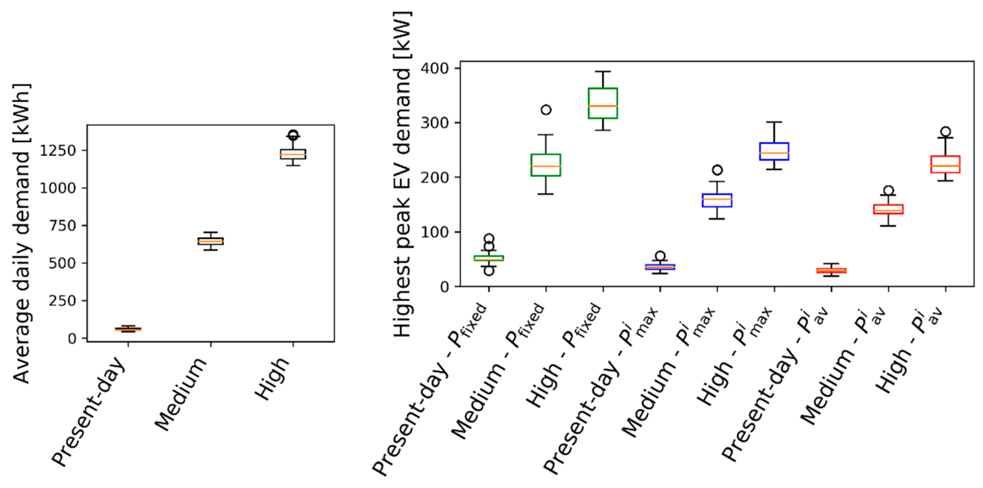
Section 2.2. The Monte Carlo simulation was carried out to investigate the spreading of the aggregated EV demand peak height and flexibility of the aggregated EV demand among different simulation runs.
3. Case Study Description
The Lombok district in the city of Utrecht, The Netherlands, has been considered as a case study. The studied area is a residential area in which a small amount of commercial activities also take place. Using the Dutch
Basisregistratie Adressen en Gebouwen (BAG)
, the following information was retrieved: 89% of the addresses is registered as purely residential; 4% has a residential function combined with another function; and the remaining 7% of the addresses are shops, offices, or other [
38]. The current car possession rate (CPR) is 0.4 HH
−1 [
39].
The EV charging data used in this study were logged at 21 charging stations located in the Lombok district over one year, from 1 August 2017 up to and including 31 July 2018. Each charging station was equipped with two charging points, both equipped with a 3 × 32 A connection on a 230 V network, so
Pmax,CP is 22 kW. This value of 22 kW is used as
for BEVs in the simulation. For PHEVs, in the simulation,
is set equal to 3.7 kW, which is the maximum charging power for the top five best sold PHEVs in the Netherlands, as mentioned in
Section 2.2. For each transaction
i, the following data are available:
: the plug-in time
: the plug-out time
: power charged at each time t during transaction i, with = 5 min
[kWh]: the total charged energy
An identity-key of each unique charging EV
Data cleaning steps included removing transactions with obvious faulty data: all transactions with = 0 s, all transactions for which > 73 h, and all transactions for which 125 kWh. The resulting dataset consists of 8223 transactions.
The area used for the simulation included 6 charging stations and 340 households. This corresponds to an area that is connected to one transformer converting medium voltage (MV) to low voltage (LV). The MV/LV-transformer in this area has a capacity limit of 400 kW.
5. Discussion
In this section, the methods and results will be discussed.
Firstly, differentiating local and visiting BEVs by setting the average energy demand at half of the average energy demand of the present Dutch BEV fleet is an arbitrary choice. However, the results show that this choice leads to a clear, and in our view realistic, approximation of the distinction between local and visiting BEVs.
Secondly, there are uncertainties in the future development of residential EV demand and the number of charging stations. Besides, the scenarios for future numbers of EVs are uncertain. This especially counts for the number of visiting EVs. However, the number of visiting EVs is expected to have a limited impact on aggregated EV demand as the charging frequency of the visiting BEVs and PHEVs is low compared with that of local ones. Further, the future number of fast charging stations, mostly next to highways or close to main roads, is difficult to predict, and will also depend on developments in EV battery capacity, which is expected to increase [
28]. A relatively large growth in the number of fast charging stations will cause the EV demand on residential networks to be lower than expected. Also, the rise of self-driving cars may result in a larger share of the EV demand being fulfilled outside residential areas, thereby decreasing the impact on residential networks.
Thirdly, there are uncertainties regarding the flexibility of the EV demand. To start with, for smart charging, active participation of EV users and their willingness to share information are of key importance. In this study, a participation of 100% is assumed. This was chosen because the target was to investigate the maximum potential flexibility and the influence of different simulation methods on estimations of future flexibility. In reality, the participation rate will be lower if the EVs are owned by individual users, causing a lower availability of the flexibility of EV demand. However, if the EVs are owned by a company, for example, a car-sharing company or leasing company, high participation rates are realistic. Further, the future charging behavior is likely to deviate from the historic measured charging data, which would influence the flexibility available. For example, the flexibility potential on residential networks may increase as a result of larger average charging power for future EVs, resulting in lower values for . Apart from this, user preferences that influence the charging scheme, such as charging part of the required energy in an uncontrolled manner and treating only the remaining energy demand as flexible load, could seriously reduce the available flexibility of EV demand. Note that user behavior may be steered if financial benefits are offered. Also, as perfect forecast is not realistic, part of the real driving behavior will deviate from the scheduled behavior. In order to avoid compromising the user comfort, ‘safety margins’ should be accounted for in the load scheduling, such as making sure that the car is fully charged a certain period before the scheduled or estimated departure time. This reduces the flexibility that can be used compared with the theoretical maximum amount of flexibility available when perfect forecast is assumed. Finally, the flexibility is influenced by the ratio between the number of EVs and the number of charging points, because charging durations are expected to decrease if charging points are more scarce. On the one hand, a high number of charging points increases the number of EVs that can charge simultaneously, which increases the maximum peak demand. On the other hand, however, a large number of charging points increases the flexibility of the EV demand, as EVs are expected to have longer connection durations when charging points are abundant compared with the situation in which charging points are scarce. In the simulation, the number of EVs charging simultaneously is left unconstrained, as it was assumed that the number of charging points is perfectly demand-driven. This was chosen because the target was to find the maximum available EV demand flexibility. In reality, the number of charging points available can be smaller, thereby limiting the available EV demand flexibility.
Fourthly, for the constraint on minimum trip duration, the maximum EV discharge power during a trip was assumed to be 20 kW, based on an average speed of 100 km·h
−1 during the trip and a driving efficiency of 5 km·kWh
−1 [
32,
37]. These numbers are uncertain as they depend on multiple variables such as the characteristics of the driving cycle and the battery technology. Yet, the exact value of the constraint is not expected to have a major impact on the results, as the constraint is not binding for most of the simulated transactions.
Fifthly, in this study, no data on home charging were available, but from our experience, this is not common in this pilot area. However, if home charging would have been included, this might have resulted in a higher demand of the current EV fleet, as well as a higher available flexibility, assuming that EVs charging at home would also be able to participate in smart charging schemes.
Further, we demonstrated that distributions of plug-in time, plug-out time, connection duration, and amount of energy charged per transaction do not follow normal distributions, suggesting that the proposed simulation method, which takes this into account, yields more realistic results compared with previous studies that use normal distributions for the simulation of one or more of these parameters.
Lastly, the different charging power simulation methods are discussed. If realistic charging profiles are not available, making a simulation using fixed constant charging power profiles is the most straightforward way to simulate EV demand flexibility. The introduction shows that many studies did indeed use a fixed constant charging power to simulate EV charging power profiles, for example, the works of [
8,
9,
11,
12,
13,
14,
16]. In this study, for BEVs, the maximum power output of the charging points of 22 kW was used as fixed constant charging power, while 3.7 kW was used for PHEVs. The results were compared to transaction-specific charging power, in the data analysis as well as in the simulation. As the fixed constant charging power was relatively high, most EVs charge with lower power in reality. Therefore, both EV peak demand and EV demand flexibility are overestimated when the maximum charging power output of the charging stations is used in simulations of future EV demand profiles. The data analysis in this study shows that for BEVs, the maximum charging power occurring during a transaction is 55% ± 25% lower than the maximum output power of the charging station of 22 kW. The average charging power during a transaction is even 67% ± 18% lower than 22 kW. Further, a large variation in transaction-specific average charging power among different transactions is observed. The battery management systems of specific EVs influence the charging power profile, as well as other factors such as outside temperature, state of charge, and battery age [
21,
22,
23]. These variations are ignored when a fixed charging power is used in simulations. To use transaction-specific average charging power for simulating the flexibility of EV demand, measured charging profiles or values for
and
must be available for each transaction and be used as exogenous input in the simulation. The advantage of this method over using the real time-varying charging profiles in the simulation, or in the EV demand scheduling, is that the computational time remains limited, while the resulting EV demand peak and flexibility closely approximate reality. For these reasons, operators of smart charging systems might require information on average charging power for each transaction, in addition to information on connection duration and required energy per transaction.
6. Conclusions
This study proposes a method for analyzing and simulating the time-dependent flexibility of EV demand. In our definition, the flexibility of EV demand is the difference between the time that the EV needs to charge, that is, the charging duration, and the time that the EV is connected to the charging station, that is, the connection duration, during a certain transaction. As a case study, we analysed the flexibility of EV charging demand using one year of measured data from charging stations located in the Lombok district, a residential area in the city of Utrecht (the Netherlands). Further, a method to simulate the future time-dependent flexibility of EV demand was proposed. Using this simulation, the differences in EV peak demand and flexibility were investigated for different scenarios and the effects of using a varying transaction-specific charging power instead of a fixed constant charging power in the simulation were tested.
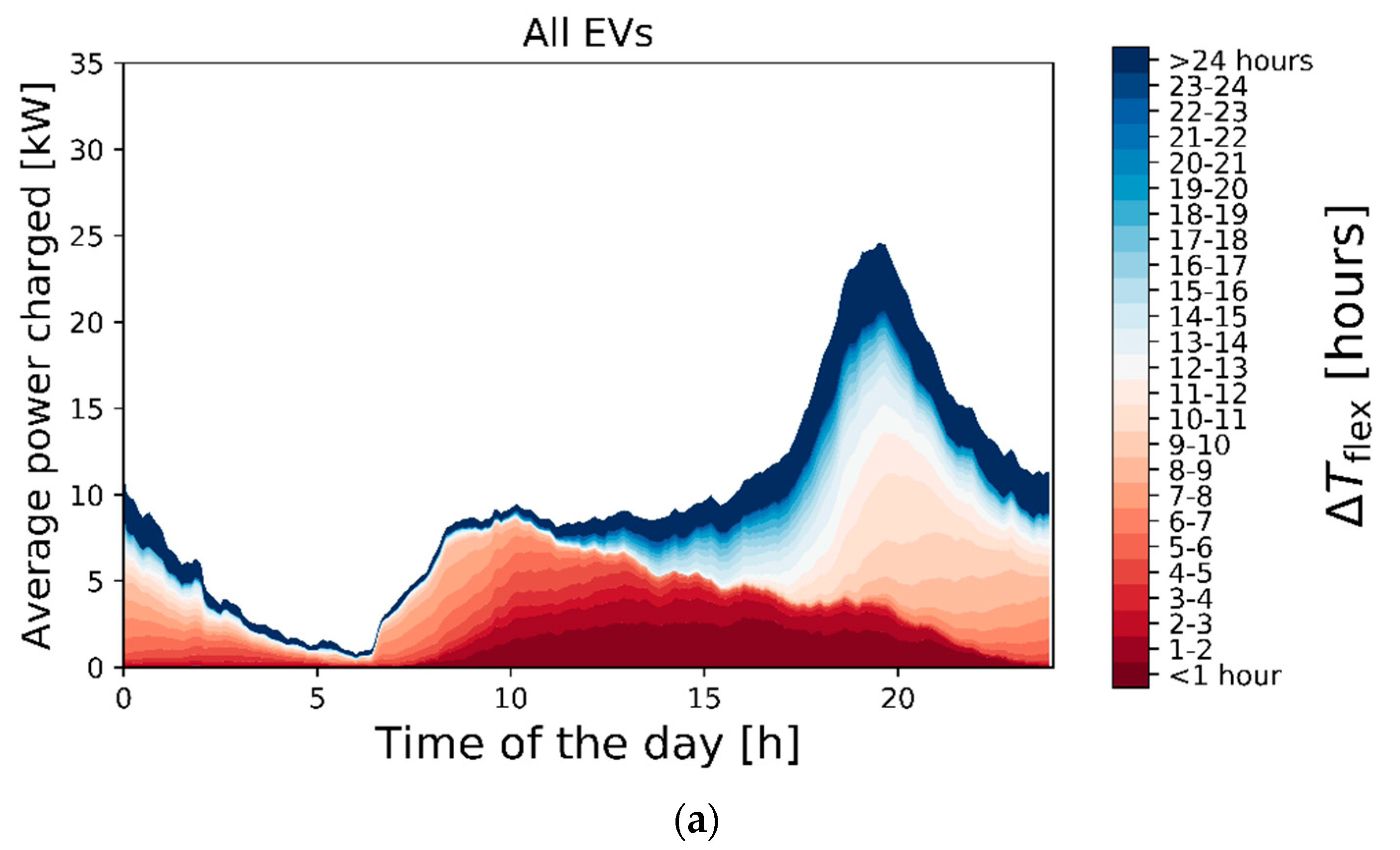
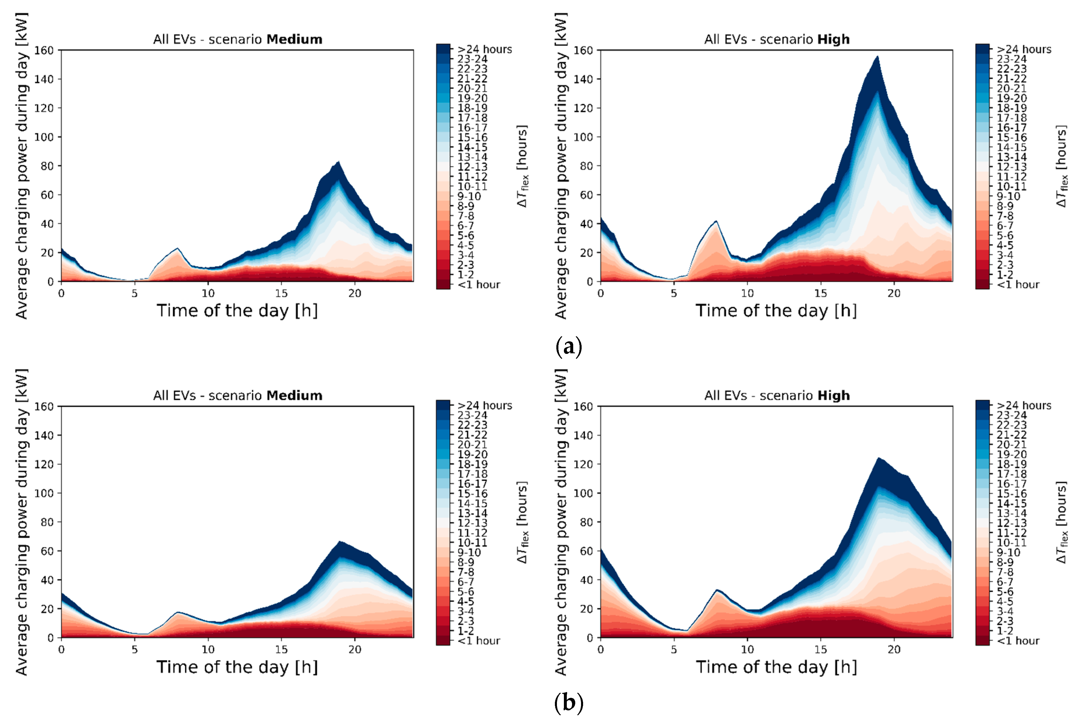
The results of the analysis of the demand flexibility in the measured transaction data show that local BEVs have a relatively high impact on the aggregated EV demand in comparison with the other EV categories, but the demand flexibility of local BEVs is also high, especially during the evening peak that occurs in the case of uncontrolled charging. The analysis shows that 59% of the present-day EV demand could be delayed over more than 8 h. Even stronger, 16% of the aggregated EV demand is flexible over more than 24 h. This suggests that there is sufficient flexibility available to charge part of the EVs during the PV generation peak of the next day.
The time-dependent flexibility is lower for the average transaction-specific constant charging power method compared with the fixed constant charging power method: 77% ± 1% of the EV demand could be delayed for more than 8 h using the fixed constant charging power method, while this figure is 64% ± 2% for the average transaction-specific constant charging power method. Further, the maximum peak demand was on average 33% lower when the transaction-specific average constant charging power method was used in the simulation instead of the fixed constant charging power method.
In future work, the results produced by the proposed methods for the analysis and simulation of EV demand flexibility can be used by smart charging models that take into account detailed flexibility constraints. A recommendation for further research is to compare different smart charging optimization algorithms, based on local photovoltaic electricity generation or electricity day-ahead and imbalance markets, while considering the flexibility constraints as described in this paper. This could shed more light on the techno–economic feasibility of different smart charging schemes. Also, it would be interesting to apply the proposed methods to investigating the flexibility of EV demand to non-residential areas, such as parking lots in the city center or near offices. Finally, the influence of charging station availability on the flexibility of EV demand could be further investigated.


