
Greenhouse Gas Savings Potential under Repowering of Onshore Wind Turbines and Climate Change: A Case Study from Germany


Environmental Meteorology, Albert-Ludwigs-Universität Freiburg, 79085 Freiburg, Germany
*
Author to whom correspondence should be addressed.
Wind 2021, 1(1), 1-19; https://0-doi-org.brum.beds.ac.uk/10.3390/wind1010001
Submission received: 9 July 2021
/
Revised: 25 August 2021
/
Accepted: 2 September 2021
/
Published: 8 September 2021
Abstract
:Wind energy is crucial in German energy and climate strategies as it substitutes carbon-intensive fossil fuels and achieves substantial greenhouse gas (GHG) reductions. However, wind energy deployment currently faces several problems: low expansion rates, wind turbines at the end of their service life, or the end of remuneration. Repowering is a vital strategy to overcome these problems. This study investigates future annual GHG payback times and emission savings of repowered wind turbines. In total, 96 repowering scenarios covering a broad range of climatological, technical, economic, and political factors affecting wind energy output in 2025–2049 were studied. The results indicate that due to more giant wind turbines and geographical restrictions, the amount of repowerable sites is reduced significantly. Consequently, in most scenarios, emission savings will dramatically diminish compared to current savings. Even in the best-case scenario, the highest emission savings’ growth is at 11%. The most meaningful drivers of GHG payback time and emission savings are wind turbine type, geographical restrictions, and GHG emissions. In contrast, climate change impact on the wind resource is only marginal. Although repowering alone is insufficient for achieving climate targets, it is a substantial part of the wind energy strategy. It could be improved by the synergies of different measures presented in this study. The results emphasize that a massive expansion of wind energy is required to establish it as a cornerstone of the future energy mix.
1. Introduction
Burning fossil fuels for power generation is one of the main contributors to global greenhouse gas (GHG) emissions leading to environmental damage and additional climate change [1,2]. Power production is responsible for about 25% of the global GHG emissions [3]. The adverse effects of fossil-based power production are reinforced with the recent high, growing global energy demand [1,4].
A meaningful way to reduce the future consumption of fossil fuels is the efficient use of renewable energies. Efficient renewable energy use is a cornerstone for reducing the negative impacts of fossil fuel combustion, achieving climate targets, and improving energy security [5].
One of the most promising renewable energy sources to phase out fossil fuels is wind energy [6]. Its meteorological and technical potential exceeds the global power and energy demand significantly [7,8]. Wind energy technologies belong to the most mature and competitive renewable energy technologies [1,4,9] able to provide clean energy [10] at competitive and low-volatile operation and maintenance costs [5,11,12,13].
Although initial costs for construction and infrastructure might be high [14], the levelized cost of energy has already reached the level of fossil fuels [15]. Concerning minimization of CO2 equivalent (CO2,eq) emissions per unit of power produced, wind energy is most promising [16]. However, although GHG emissions during the operation phase of wind turbines are negligible [1], wind energy technologies are not emission-free from a life cycle perspective.
The CO2,eq emissions of wind turbines during their service life can be quantified by a life cycle assessment (LCA). LCA is used to evaluate the environmental impacts of a technology or service considering all resources and energy required during all stages of wind turbines’ life cycles [1,17].
The life cycle of wind turbines mainly comprises the stages of raw material extraction, manufacturing/production, transportation, installation, operation, maintenance, dismantling, disposal, or recycling. In general, production, including raw material extraction and construction, is responsible for most of a wind turbine’s life cycle GHG emissions [1,16,18,19,20]. Depending on the distance between wind farm site and wind turbine production site, transport emissions might become superior [6]. Wind turbine recycling can contribute to up to 20–30% GHG emission reductions [16,18,21].
Overall, GHG emissions during wind turbines’ service life mainly depend on (1) the production conditions and manufacturing process, (2) the product design and size, and (3) local wind conditions. GHG emissions vary greatly depending on the geographical locations of the manufacturing [1,22]. The more carbon-intensive the power mix of a production country, the more emissions arise during this stage [18,23]. In a previous study [18], it was demonstrated that the same manufacturing process would lead to less than half of the emissions in Germany compared to China.
Different LCAs have illustrated that total emissions of wind energy technologies are highly correlated with the size and design of wind turbines. Depending on wind turbine type, wind turbine properties, and location, the life cycle GHG emissions of onshore wind energy range between 1.7 and 123.7 gCO2,eq/kWh with the mean being 34.2 gCO2,eq/kWh. Mean life cycle emissions (1054 gCO2,eq/kWh) of lignite power plants are up to 30 times higher per power unit. Wind energy does not only perform better than fossil energies but is also advantageous compared to other renewables. The life cycle emissions of photovoltaic systems are most often higher than those of wind turbines [23]. However, synergies of different renewables will be required to achieve national and global climate targets as especially wind and solar are highly volatile energy sources.
Increasing dimensions lead to higher life cycle emissions as more carbon-intensive materials such as steel and concrete are needed. Still, the specific GHG emissions might decrease as more giant turbines are more productive. Furthermore, there are differences between turbines with horizontal and vertical axes [24]. Onshore and offshore wind turbines differ in their life cycle GHG emissions. The emissions of offshore wind turbines are higher than those of onshore turbines due to higher material and energy inputs, including those from transmission cables or the floating platform [1,6,25,26].
Due to the emissions arising in some life cycle stages, a wind turbine does not contribute immediately to net GHG savings during its service life. A certain amount of time is required until the GHG savings of a wind turbine replacing conventional power plants exceeds GHG emissions originating from the wind turbine itself. This time is called greenhouse gas payback time (GPBT) [17,27]. Only after this time, a wind turbine contributes to net GHG emission savings.
GHG savings and GPBT depend on wind turbines’ properties, energy yield, and the replaced technologies and GHG emissions during their life cycle. GHG emissions of conventional power plants mainly arise during their service life as direct emissions from the combustion of fossil fuels [16,18,19] and differ depending on the type of fossil energy source and the efficiency of a power plant [28]. The higher the carbon content of a fossil-based energy source, the higher its GHG emissions. Therefore, coal-based power plants emit more GHG emissions than oil or natural gas technologies.
The overall GHG emissions savings through wind energy can be quantified via a net-emission balance considering life cycle GHG emissions of wind energy and conventional energy sources. The replacement of more carbon-containing fossil fuels contributes to higher GHG savings. Thus, more decarbonized societies will not profit that much from additional wind energy deployment as a highly carbon-based country [29].
The actual order of replacement is mostly rather an economic and technical than ecological question. The merit order determines which energy sources are replaced first, depending on their costs. According to the current German and European merit order, wind energy will replace natural gas, hard coal, and partly lignite power plants soon [30]. In previous studies [28,31], it was assumed that, first of all, more flexible power plants such as natural gas can be replaced. In contrast, coal-based power plants can only be replaced with lower overall power consumption and higher wind energy output.
In Germany, wind energy plays a crucial role in increasing renewables, avoiding GHG emissions, and reaching climate targets [32]. In 2020, with an installed capacity of 54.4 GW, wind energy made up 52% (onshore 41.3%) of the German renewable power production, avoiding 101 MtCO2,eq (onshore: 80 MtCO2,eq) of GHG emissions [33]. However, the current expansion rate of German wind energy capacity is low [34], and many wind turbines are at the end of their service life. They will be affected by the expiry of remuneration (after 20 years) initiated by the Renewable Energies Act [32]. Repowering is one way of dealing with ageing wind turbines without exploiting new sites [35].
To quantify the GHG savings potential of repowering on local and national scales, this study applies, synthesizes, and extends a variety of previous findings by considering climatological, technological, political, and economic aspects. A multi-scenario approach is used to handle uncertainties related to future development and it provides future projections of wind energy deployment.
Using wind data from climate models provided by the European branch of the international CORDEX initiative (EURO-CORDEX) and different scenarios regarding wind turbine types, geographical restrictions, and emission reductions, this study addresses the following questions: (1) Does global climate change affect the overall wind energy output, GPBT, and GHG emission savings of wind turbines and their spatial variability in Germany? (2) Does nationwide repowering of the current wind turbine fleet suffice to increase the amount of wind energy production and GHG emission savings to reach the national climate targets? (3) Which measures can be taken to improve future GHG savings? The answers to these questions are based on evaluating 96 repowering scenarios (S1–S96) under which the future quality and quantity of repowerable German onshore wind turbine sites in terms of their GPBT and GHG emission savings potential were studied.
The results of this study provide a valuable basis for environmental policy makers from the local to the national scale. In addition, they assist wind turbine operators in evaluating the benefits of repowering wind turbines from both an energy yield and greenhouse gas-saving perspective. The methods presented are transferable to other study areas and allow research to be applied.
2. Materials and Methods
2.1. Workflow
The assessment of GPBT and annual GHG savings (AS) included the following main steps (Figure 1): (1) assembling of the year 2020 wind turbine fleet in Germany, (2) application of four different generic wind turbine types (WTTs) with a service life of 25 years, (3) assessment of repowerable sites applying the geographical restriction criterion (GRC) and the wind turbine spacing criterion (WTSC), (4) simulation of a nationwide repowered wind turbine fleet in 2025, (5) calculation of wind speed in a hub height of 140 m (hhub) with bias-adjusted EURO-CORDEX data (Uhub), (6) quantification of the mean annual wind energy yield at the wind turbine sites (AEYWT), (7) determination of WTT-specific life cycle GHG emissions (GGAWTT), (8) definition of four different power mix benchmarks (ES1-ES4), (9) calculation of turbine-specific GPBT (GPBTWT), (10) calculation of turbine-specific AS (ASWT), and (11) summation of ASWT to determine cumulative AS in the study area (ASC). The calculation of GPBTWT and ASWT was made under S1–S96.
2.2. Study Area
The study was carried out in Germany, stretching over 357,376 km². The predominant land-use types in the study area are agricultural areas (59%), forests (30%), and artificial surfaces (8%) [36]. Compared to the other parts of the study area, the northwest is flat and less forested. The highest mean wind speed at hhub in 1979–2014 ( > 7.0 m/s) can be found near the North and Baltic Sea coasts in the north and further inland within about 30 low mountain ranges of which 91% rise to a maximum of 1200 m above sea level (Figure 2). There is a pronounced large-scale north-south gradient in the pattern. The lowest values of < 2.0 m/s occur in the Alpine foothills in the southeastern parts of the study area [37].
The basis for this analysis was comprehensive data on 27,939 onshore wind turbines installed in the study area at the beginning of 2020, including information on wind turbine location, hhub, rated power (Pr), total wind turbine height (H), rotor diameter (D), and years in operation [32]. While most wind turbine sites are in the northwestern part of Germany, the southern part has relatively few installations.
2.3. Estimation of Energy Yield
The recent wind resource in the study area was estimated by applying the wind speed-wind shear model (WSWS) [38]. The model was parameterized at a 200 m × 200 m horizontal resolution allowing a three-dimensional wind resource assessment in the altitude range 10–200 m.
A multi-model ensemble of near-surface (10 m) wind speed time series at a daily resolution for 1981–2099 from 29 different global-regional climate model combinations was used to assess the future spatiotemporal variations of the wind resource [39]. Using WSWS, the time series representing the future near-surface wind speed conditions were bias-corrected via quantile-matching and extrapolated to hhub at the sites of the current wind turbines included in this study.
Four generic power curves were chosen from a wind turbine library [40]. The library contains information on the specifications and dimensions of 140 wind turbine types. Properties of the four selected WTTs are presented in Table 1.
Using the approach reported in a previous study [41], air density-corrected AEYWT was calculated using
with n being the number of hours, d the number of days in a year, and PWT(Uhub,i) being wind power associated with Uhub on the day i. To consider the downtime of wind turbines, the turbine availability (WTA) was assumed to be 0.97, which is a typical value for Germany [42]. The wind farm efficiency (WFE) accounts for wake effects due to neighboring wind turbines, which was assumed to be 0.95.
2.4. Geographical Restrictions
According to German legislation, not all onshore sites of the current wind turbine fleet can be repowered [32]. Especially the distance requirements between wind turbines and settlements will significantly diminish the number of eligible sites. Moreover, those distances are not standardized and highly debated.
To estimate the impact of the distance regulations on the future development of AEYWT in the study area, three currently used distances to settlements were employed as variants of the geographical restriction criterion (GRC). The first variant of GRC simulates weak restrictions with a minimum distance of 500 m to the next settlement (GRC-W). Moderate restrictions with a minimum distance of 1000 m to the next settlement were considered via GRC-M. The strictest variant GRC-S is based on H. It represents a strongly restrictive scenario with a 10H minimum distance to the next settlement, taking up the most rigorous rules to be found in the study area [45].
Additionally, the spacing between wind turbines was considered. The wind turbine spacing criterion (WTSC) was set to five times turbine-specific D. In a stepwise procedure, AEYWT was compared in the study area. Less productive sites within a distance of less than 5D of the wind turbine under investigation were step-by-step eliminated.
2.5. Greenhouse Gas Payback Time and Annual GHG Savings
Based on AEYWT of the repowerable wind turbines, GPBTWT was calculated. It quantifies the time required until GHG savings of a wind turbine exceed GHG emissions originating from the wind turbine’s life cycle [17]:
where GGAWTT are the cumulative life cycle GHG emissions of a wind turbine (gCO2,eq/turbine), and GGAPM represents the specific GHG life cycle emissions of the power mix benchmark (gCO2,eq/kWh).
GGAWTT depends on wind turbine properties. It was calculated for WTT1-WTT4. By applying the regression model reported in a previous study [17], GGAWTT was determined as a function of D and hhub:
with c0 = 2.00, c1 = 1.27, and c2 = 0.84.
Dividing the 25-years sum of AEYWT for each wind turbine by the number of lifetime months (in this case 300), PWT was quantified. To assess the impact of ES1–ES4, four power mix benchmarks were used (Table 2).
ES1 and ES4 are based on rounded emission factors of the power mix in 2019 and 1990 [46]. ES2 and ES3 use power mix benchmarks calculated as a weighted mean in a power mix of different conventional energy sources. While the ES2-related power mix benchmark excludes renewable energies (value refers to 2019), ES3 considers the onshore wind energy substitution [30].
In ES2 and ES3, the share of each energy source was multiplied by the specific life cycle GHG emissions of conventional energy sources (Table 3) reported in an earlier study [23].
The power mix benchmarks were established as it remains uncertain which energy sources will be replaced soon in Germany. Wind energy may replace carbon-intensive as well as low-carbon technologies.
Using AEYWT, GGAPM, and GGAWTT, ASWT was calculated according to the following equation:
with LT representing the length of wind turbines’ service life. By summing up the mean ASWT values, ASC was quantified.
Based on the difference between future annual energy yield (AEYC,F) to energy yield of 2019 (AEYC,2019 = 101.2 TWh [47]), and by applying GGAPM, the difference in GHG savings (ΔASC) in the study area was estimated:
The 29 analyzed combinations of global and regional climate models (M1–M29) under the Representative Concentrations Pathway scenarios RCP4.5 and RCP8.5 are summarized in Table S1 in the Supplementary Materials. The RCP scenarios summarize potential developments of the global future climate. The values of 4.5 and 8.5 represent an anthropogenic additional radiative forcing in 2100 compared to 1850 [48]. The RCP8.5 scenario is thus the scenario with the higher anthropogenic greenhouse gas emissions. The assumptions for S1–S96 are listed in Table S2.
3. Results and Discussion
3.1. Repowerable Sites
The current wind turbine fleet includes turbines at sites that are not repowerable due to German legislation. By applying GRC-W, the repowerable sites are reduced to 96.1% (Table 4). The use of GRC-M chops the eligible sites to 79.1%. Since GRC-S depends on H, it significantly reduces the authorized sites to 28.5–39.5%, depending on WTT.
The application of WTSC shows an even more substantial effect. Depending on the repowering scenario, the share of wind turbines decreases to 8.1–37.6%. With applying WTSC, no significant difference between the two RCP scenarios arises, indicating that the potential energy yield for 2025–2049 is similar for most sites.
The strong effect of repowering in reducing the wind turbine fleet was also reported in an earlier study demonstrating that only half of the wind turbine fleet is within repowerable areas. In that study, the share of repowerable areas decreased to below 35% with a national settlement distance regulation of 1000 m [49].
These results are similar to the values shown in S9–S16, which is also based on the same distance requirements. In general, the impact of settlement distance requirements is extraordinarily high compared to other restrictions [50], and an increase in distance requirements decreases the energy potential significantly [51]. Small WTGRC associated with S89–S96 is caused by the combination of strict geographical restrictions and large dimensions of WTT4.
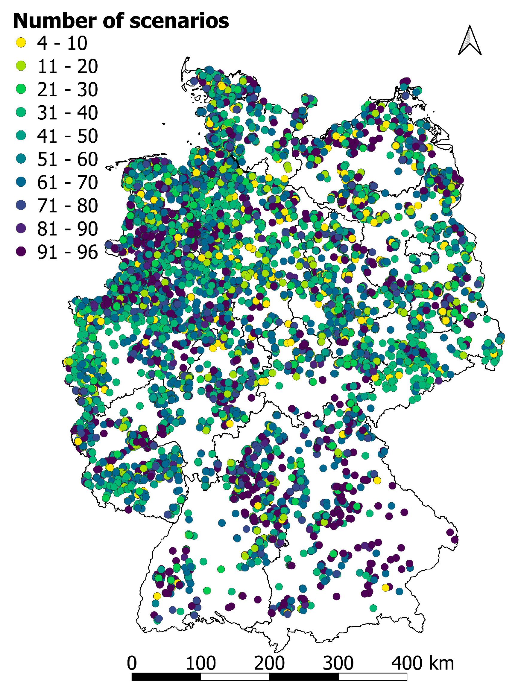
For all assessed wind turbine sites, the number of scenarios under which they are classified as repowerable is shown in Figure 3. The number of scenarios is a patchwork throughout the study area. There is no region in which a pronounced scenario-related systematic is dominant. This is mainly due to the diverse mix of regional wind resources and settlement structures in the study area.
Most of the sites fall into the class 61–70 scenarios, as indicated by the legend. About 8.3% fall into the lowest class 4–10 scenarios, while 15.0% of the sites are repowerable in at least 91 scenarios. From the original wind turbine fleet, 57.1%, i.e., 15,955 turbines, cannot be repowered in the scope of this study.
3.2. Greenhouse Gas Payback Times of Wind Turbines
The GPBTWT pattern in the study area associated with the worst-case scenario (S18) results from the combination {RCP8.5, WTT1, GRC–S, ES1} (Figure 4). Under this scenario, the share of wind turbines with GPBTWT > 7 months is 100% and therefore significantly higher than under any other scenario. The share of GPBTWT > 12 months amounts to 71%.
The best-case scenario (S80) is the outcome from the combination {RCP8.5, WTT4, GRC-W, ES4}. Only 1% of the wind turbines have GPBTWT > 7 months. The share of wind turbines with less than 5 months is around 80%. For better comparison, all three scenarios refer to the same climate change scenario.
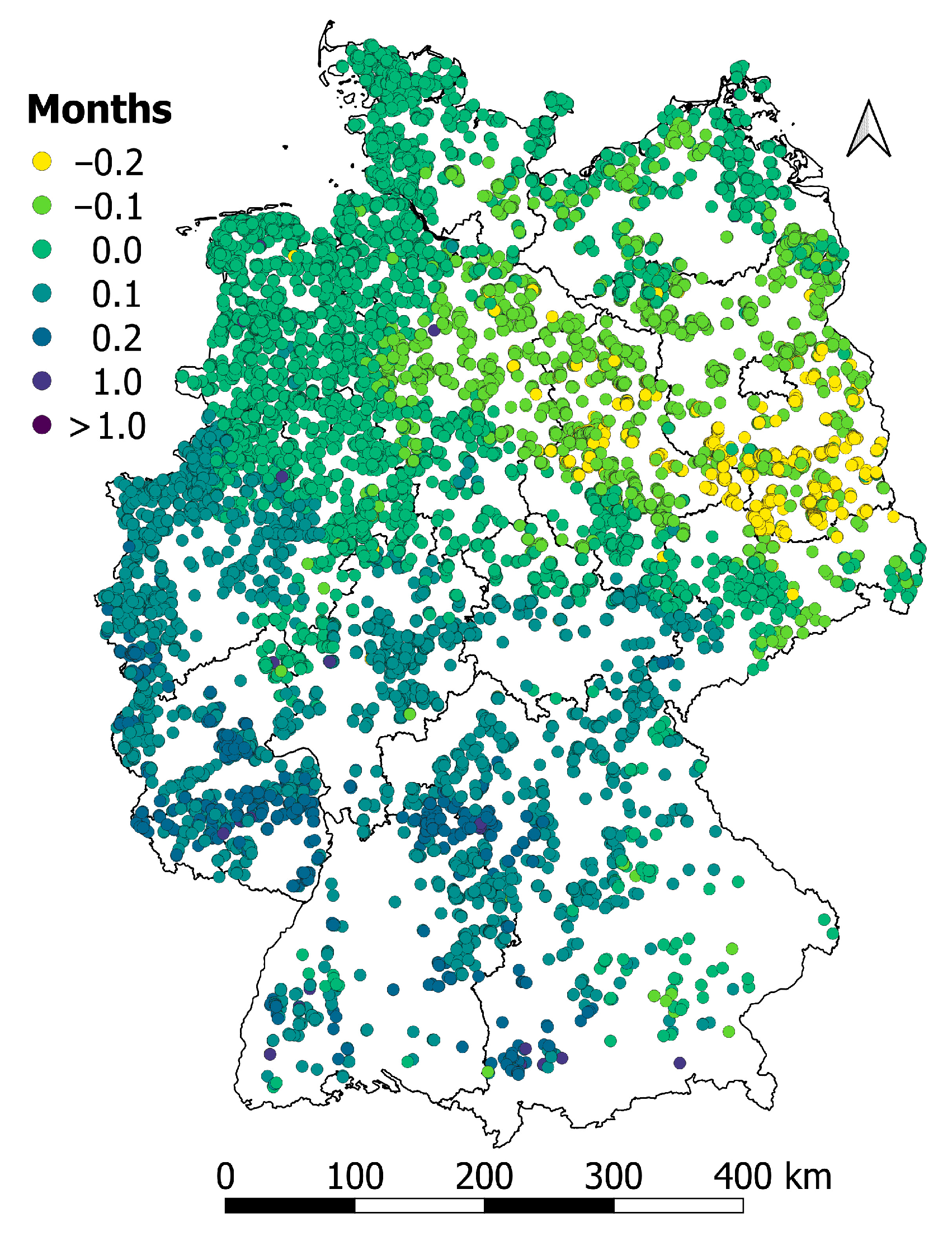
The median difference of GPBTWT between RCP8.5 and RCP4.5 (ΔGPBTWT) is mostly marginal (Figure 5). It varies in the range of −2.4 to 2.6 months. The majority of the values lie between −0.2 and 0.1 months. This indicates a weak impact of the evaluated climate change scenarios on future GHG payback times. Different climate change scenarios project relatively small changes in the mean wind energy output in Europe. However, wind energy production depends on atmospheric conditions and thus could be potentially affected by climate change. There is a high uncertainty between the climate models concerning magnitude- and sign-related changes in the wind resource [48]. As used in this study, a multi-model approach is generally the best way to handle model-related uncertainties [52]. However, while changes in mean wind energy output are relatively small, climate models indicate that the inter- and intra-annual variabilities might change significantly [48,52,53]. Both aspects potentially affect the GHG payback times as periods with low wind availability could extend GPBT.
The spatial ΔGPBTWT pattern exhibits a weak, large-scale tendency towards greater ΔGPBTWT values from the northwestern to southwestern turbine sites. Most negative ΔGPBTWT values are found in a narrow band in the eastern parts of the study area. In the very south, sites where ΔGPBTWT = 0.0 months might neighbor sites where ΔGPBTWT > 1.0 months.
Since the differences in climate change scenario-related GPBTWT are extremely small, they are not considered to affect the repowering strategy in this study. However, climate change might affect regions in the study area differently. The higher ΔGPBTWT values in the southern and southwestern parts indicate that under RCP8.5, wind energy yield is projected to decrease, leading to higher GPBTWT compared to RCP4.5.
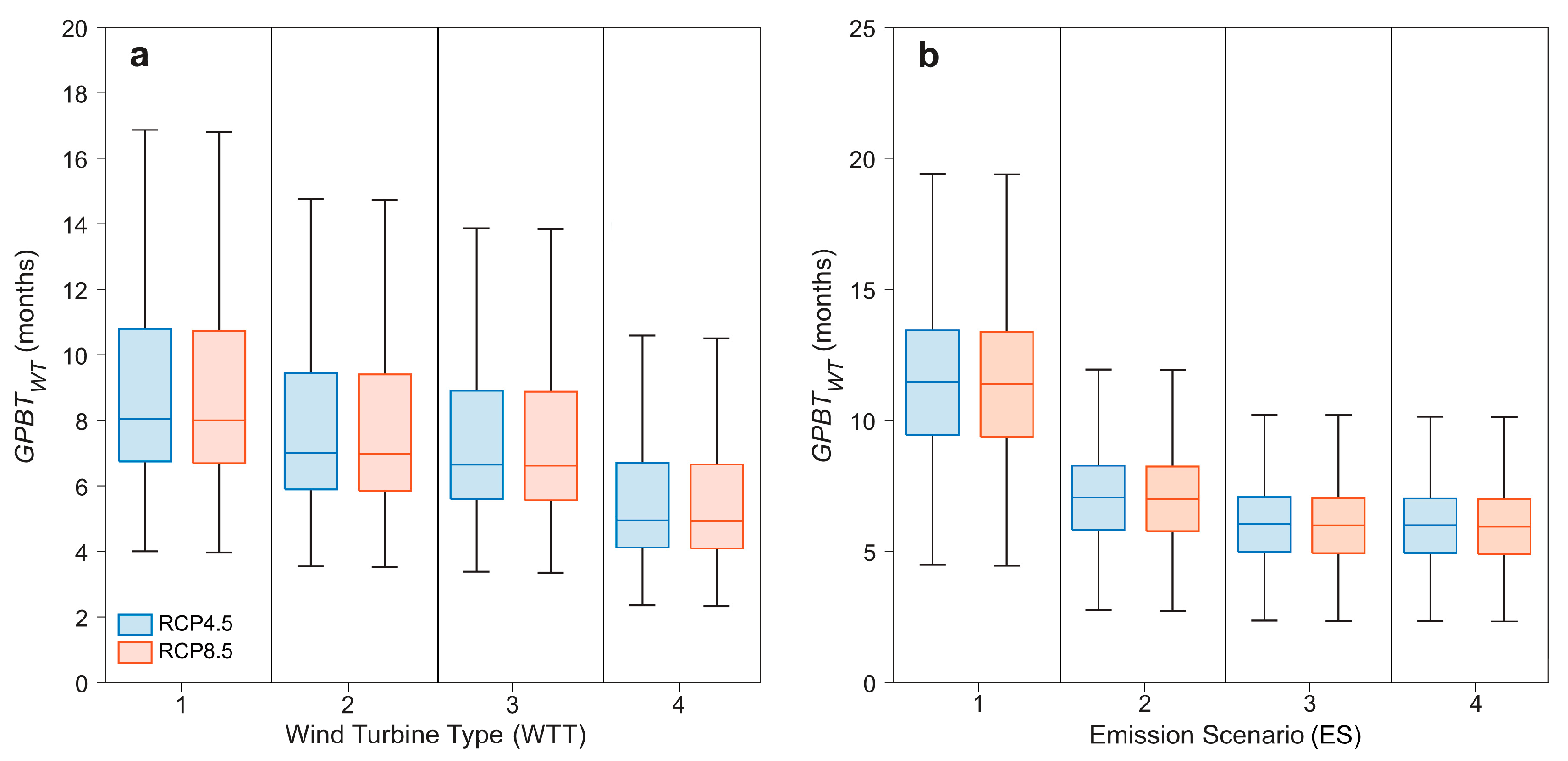
The wind turbine type-specific GPBT at the wind turbine level decreases from WTT1 to WTT4 (Figure 6). There are no significant (α = 0.05) differences in the medians between RCP8.5 and RCP4.5, indicating that WTT and not the projected climate change dominates future GPBTWT development. Depending on WTT, median GPBTWT varies from 4.9 (interquartile range of 4.1 to 6.7 months) to 8.0 months (interquartile range of 6.7 to 10.8 months), with WTT4 exhibiting the lowest median values of 4.9 months under RCP8.5 and 5.0 months under RCP4.5. The presented GPBT values are in accordance with the findings from an earlier study [17], which calculated a GPBT of 1.8 to 22.5 months (mean: 5.3 months) for wind turbines in northwestern Europe.
Under ES1, the median GPBTWT of 11.5 months is almost 2.0 times higher than the ES3- and ES4-related median GPBTWT of 6.0 months. ES1- and ES2-related GPBTWT medians differ significantly from each other and ES3 and ES4 medians. In contrast, the GPBTWT medians under ES3 and ES4 show no significant difference. This is due to a more negligible difference in GGAPM between ES3 and ES4 of 5.0 gCO2,eq/kWh.
The different emission scenarios account for the uncertainties related to future life cycle emissions and power mix benchmarks. In fact, GGAPM and life cycle emissions are not constant as assumed in this study, but very dynamic [29]. On the one hand, GGAPM might decrease if society becomes more decarbonized. On the other hand, feedback mechanisms due to an increasing share of renewables might reduce the carbon intensity of materials used for wind turbine constructions. Therefore, life cycle emissions of each wind turbine decrease while saving potentials increase. Unfortunately, there is a high uncertainty related to the GHG intensity of materials and life cycle processes [6]. The future GGAPM development is a technological and economic issue as the merit order determines the substitution process [30].
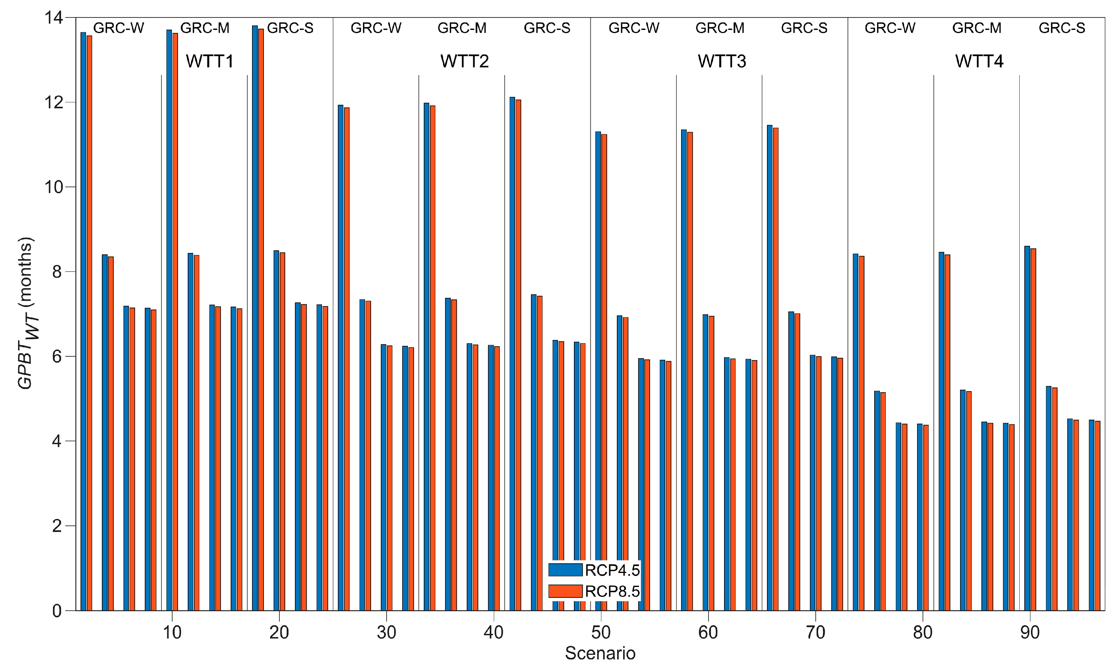
The compilation of mean GPBTWT values associated with S1–S96 reveals the dominant impact of ES, GRC, and WTT features on the projected GPBTWT development (Figure 7). Whereas there are no significant differences between RCP4.5 and RCP8.5, GPBTWT significantly decreases with increasing WTT and ES and slightly increases with stricter GRC scenarios.
The effect of GRC on GPBTWT is weak, as GRC controls the quantity but not the quality of wind turbine sites. The most potent effect is shown between ES1 and ES2. Power mix benchmarks are therefore essential factors determining future GPBTWT. In total, the mean values of GPBTWT range from 4.5 months (S96) to 13.8 months (S17). Wind turbines contribute to net GHG savings in most scenarios after a short timeframe of fewer than 12 months.
3.3. Annual GHG Savings of Wind Turbines
The ASWT pattern associated with the worst-case scenario (S18) results from the combination {RCP8.5, WTT1, GRC-S, ES1}. Under this scenario, the amount of wind turbines is significantly reduced compared to the other scenarios, and the maximal value of ASWT is only 3.3 ktCO2,eq. Most values are smaller than 2.5 ktCO2,eq (Figure 8).
The best-case scenario (S80) is the outcome from the combination {RCP8.5, WTT4, GRC-W, ES4} and shows significantly higher ASWT reaching up to 21.3 ktCO2,eq, and 41% of the values are higher than 12 ktCO2,eq. In all scenarios, the highest ASWT occurs in the study area’s northern and northwestern coastal zones.
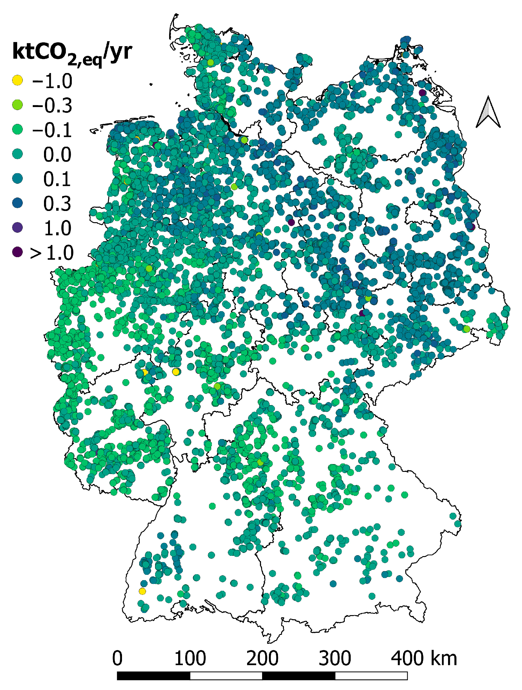
The values of ΔASWT are mostly small (Figure 9). In a few extreme cases, they reach −6.1 to 6.2 ktCO2,eq. However, the majority of the values range from −0.3 to 0.1 ktCO2,eq. This indicates again a generally weak impact of the evaluated climate change scenarios on future ASWT. Complementary to the patterns of ΔGPBTWT, the variability of ΔASWT exhibits a weak, large-scale tendency towards lower ΔASWT values from the northeastern to southwestern turbine sites. Values in the lowest class with ΔASWT < −1.0 ktCO2,eq only rarely occur. In the south and southwest of the study area, sites with high ΔASWT might neighbor sites with low ΔASWT.
3.4. Annual GHG Savings in the Study Area
The impact of the climate change scenarios on mean ASC is marginal and non-significant (α = 0.05), as shown in Figure 10. These results are plausible with the background of only small projected changes in the mean future wind energy output under climate change [48,52]. However, the inter-annual variability of ASC might be affected by climate change-induced shifts in the wind energy output [48,52,53].
The differences in S1–S96 mainly result from the combination of WTT, GRC, and ES. In general, with stricter distance to settlement regulations, ASC becomes significantly smaller, especially using WTT4 due to the 10H rule. Within the scenarios with the same distance regulations, ASC is always greatest using WTT4. The emission scenario leading to the most significant mean ASC values is ES4, although only with a slight difference to ES3, e.g., 75.7 (S80) to 75.2 (S78) MtCO2,eq.
The lowest mean ASC is connected with ES1, independent of the WTT and GRC scenario. The presented values are within the range of a previous study [54], which estimated ASC between 45.6 and 76.3 MtCO2,eq based on the inter-annual variability of the wind resource. The mean values of ASC are all lower than the current level of annual GHG savings in the study area (79.7 MtCO2,eq) [33].
The aggregated future GHG savings on the national level depend primarily on WTT (Figure 11). The effect of the underlying climate change scenario is not significant. The turbine type-specific ΔASC medians and the associated interquartile ranges are almost identical, with the median GHG savings under RCP8.5 being slightly higher for WTT1-WTT3 (−38.8 to −29.6 MtCO2,eq) than under RCP4.5 (−39.4 to −30.0 MtCO2,eq). For WTT4, the ΔASC median of RCP4.5 is slightly higher (−10.0 MtCO2,eq) compared to RCP8.5 (−10.2 MtCO2,eq).
The most considerable GHG savings by far were quantified for WTT4, 7.2 MtCO2,eq under RCP4.5 and 8.5 MtCO2,eq under RCP8.5. With WTT4, ASC exceeds the current state of annual GHG savings within some years and scenarios (>0.0 MtCO2,eq). Compared to ASC = 77.8 MtCO2,eq in 2019 [33], this corresponds to an increase of 11%.
As shown in Figure 10, these values do not occur if the scenario mean values are considered for all years. Compared to the other WTTs, WTT4 represents a somewhat hypothetical wind turbine type. It is not expected that comparable WTTs with such high rated powers and large rotor diameters will soon be used nationwide for onshore wind power generation. WTTs with rated power up to a maximum of 8 MW occur in the current onshore wind turbine fleet, but those are very rare. Only 1% of the existing wind turbines have a rated power higher than 4 MW [32].
With all other investigated WTTs, ASC is significantly lower than the current level, leading to decreased GHG savings under repowering. Accordingly, repowering alone is unable to maintain or even increase future ASC.
Without an expansion of the wind turbine fleet, the contribution of wind energy to the energy mix in the study area will constantly diminish [32].
As summarized in Table 5, GPBT, ASWT, and ASC are influenced by several drivers, represented by S1–S96. Those scenarios comprise assumptions about the climatological (RCP), technical (WTT, ES), political, social, and economic aspects (ES, GRC). Synergies of all those different aspects will determine the future wind energy deployment and the achievement of national and international climate targets [15].
The most critical drivers in S1–S96 are WTT, ES, and GRC. The effect of climate change on the mean wind energy use under RCP4.5 and RCP8.5 is projected to be small. Therefore, within 25 years, ASC is only marginally affected by climate change, as shown in the results. However, increasing intra- and inter-annual variability of the wind energy output as projected by climate models might affect GPBT, ASWT, and ASC within shorter timeframes. Additionally, our results indicate that spatial patterns of ASWT and GPBT could change slightly.
Technological aspects that could contribute to higher GHG savings and improved energy security are increasing wind turbine dimensions, extended wind turbine lifetime, a higher share of offshore wind energy, and expanding the power grid [7,8,9,16,18,21,55].
Following a previous study [32], the results emphasize the necessity of a substantial expansion of the wind turbine fleet to increase the share and GHG saving potential of wind energy in the study area as repowering alone is not sufficient to maintain or even increase the current level of annual GHG savings.
Relying only on the current wind turbine fleet endangers the binding GHG reduction targets in the energy sector. According to the German targets, the energy sector can emit a maximum of 175–183 MtCO2,eq in 2030 [56]. In 2020, GHG emissions in the energy sector were 280 MtCO2,eq [57]. Therefore, the gap between the current state and the climate target of 2030 amounts to 97–105 MtCO2,eq. In 2020, 79.7 MtCO2,eq were avoided by onshore wind energy in the study area [33]. With repowering, this amount would be replaced by ASC.
If one assumes ASC = 32 MtCO2,eq, which is the average across all S1–S96-related GHG savings at the national level, instead of the current amount of 80 MtCO2,eq, the gap increases to 145–153 MtCO2,eq. With a mean ASWT of 5 ktCO2,eq, about 30,000 additional wind turbines would be required to fulfill the climate target for 2030 in the energy sector if the share of other renewables remains stable. However, space for installing new onshore wind turbines is scarce [49].
To maximize the climate-related benefits of wind energy and other renewable energy technologies, the use of RE sources has to be coupled with reduced energy demand [7].
4. Conclusions
This study assessed Germany’s future wind turbine-specific GHG payback times and greenhouse gas emissions savings. The calculation of the payback times and emission savings was performed based on CORDEX climate model data for 2025–2049. In total, 96 repowering scenarios were investigated, comprising different assumptions on climatological, technical, economic, and political aspects of future wind energy deployment.
The results indicate that climate change affects wind energy output, GHG payback times, and emission savings only marginally regarding the study period. However, the spatiotemporal distribution of wind energy output in the study area might change under climate change, potentially altering the GHG balance within specific regions or resulting in shorter timeframes.
In contrast, the choice of wind turbine type, geographical restrictions, and emission scenarios had substantial impacts on future GHG payback times and emission savings. While the wind turbine type and the emission scenarios determine local values at the wind turbine level, geographical restrictions control annual emissions savings at the national scale by regulating the number of repowerable sites.
Although repowering of the current wind turbine fleet leads to more efficient exploitation of the wind resource, this study calculates that repowering alone is not able to maintain or even increase the current level of GHG savings in Germany, which is caused by a massive reduction of eligible wind turbine sites due to geographical restrictions. Even in the best-case scenario, future GHG savings might exceed current savings only in a few years. The maximum value of total GHG emission savings is 11% higher compared to the current level.
These findings emphasize that wind energy repowering alone significantly falls short in reaching the national climate targets of the energy sector in Germany. Up to 30,000 additional wind turbine sites will be required to fulfill the German climate targets for 2030 if the level of other renewable energy technologies remains stable.
Nevertheless, repowering of the current wind turbine fleet should be a crucial part of the future wind energy strategy as it reduces land requirements and time-consuming selection of new appropriate sites. The results of this study provide a multitude of measures that can be taken to improve future repowering-related GHG savings. Among these are the choice of appropriate, modern wind turbine types, substitution orders reflecting the technical aspects, economic possibilities and GHG intensity of different fossil fuels, less strict geographical restrictions, and decreasing energy demand. These aspects have to act synergistically to maximize the benefits of wind energy.
Supplementary Materials
The following are available online at https://0-www-mdpi-com.brum.beds.ac.uk/article/10.3390/wind1010001/s1, Table S1: Combinations of global (GCM) and regional (RCM) climate models (M1–M29) as well as analyzed model run under the climate change scenarios RCP4.5 and RCP8.5. Table S2: Characteristics of the 96 evaluated repowering scenarios (S1–S96), including climate change scenarios (RCP), wind turbine type (WTT), geographical restriction criterion (GRC), and emission scenario (ES).
Author Contributions
Conceptualization, L.S., C.J. and D.S.; methodology, L.S., C.J. and D.S.; software, L.S., C.J. and D.S.; validation, L.S., C.J. and D.S.; formal analysis, L.S., C.J.; resources, D.S.; data curation, L.S., C.J. and D.S.; writing—original draft preparation, L.S.; writing—review and editing, L.S., C.J. and D.S.; visualization, L.S., C.J. and D.S. All authors have read and agreed to the published version of the manuscript.
Funding
This research received no external funding.
Institutional Review Board Statement
Not applicable.
Informed Consent Statement
Not applicable.
Data Availability Statement
Data available on request from the authors.
Conflicts of Interest
The authors declare no conflict of interest.
Nomenclature
| Acronyms | Description |
| AEYC,2019 | annual wind energy yield in the study area in 2019 (Wh) |
| AEYC,F | future annual wind energy yield in the study area (Wh) |
| AEYWT | mean annual wind energy yield at a wind turbine site (Wh) |
| AS | annual greenhouse gas savings (gCO2,eq) |
| ASC | annual greenhouse gas savings in the study area (gCO2,eq) |
| ASWT | annual greenhouse gas savings at a wind turbine site (gCO2,eq) |
| d | number of days in a year |
| D | rotor diameter (m) |
| GGAPM | life cycle greenhouse gas emissions of the power mix benchmark (gCO2,eq) |
| GGAWTT | wind turbine type-specific life cycle greenhouse gas emissions (gCO2,eq) |
| GPBT | greenhouse gas payback time (month) |
| GPBTWT | greenhouse gas payback time at wind turbine sites (month) |
| GRC | geographical restriction criterion |
| H | total wind turbine height (m) |
| hhub | hub height (m) |
| LT | wind turbine’s service life (yr) |
| n | number of hours |
| Pr | rated power (W) |
| PWT | wind power (W) |
| Uhub | wind speed at hub height (m/s) |
| average wind speed at hub height (m/s) | |
| WFE | wind farm efficiency |
| WTA | wind turbine availability |
| WTSC | wind turbine spacing criterion (m) |
| Abbreviations | Description |
| CORDEX | Coordinated Regional Climate Downscaling Experiment |
| ES1-ES4 | emission scenarios 1 to 4 |
| GHG | greenhouse gas |
| GPBT | greenhouse gas payback time |
| LCA | life cycle assessment |
| RE | renewable energy |
| RCP | Representative Concentration Pathways |
| S1–S96 | repowering scenarios 1 to 96 |
| WSWS | Wind Speed-Wind Shear model |
| WT | wind turbine |
| WTT | wind turbine type |
References
- Bhandari, R.; Kumar, B.; Mayer, F. Life cycle greenhouse gas emission from wind farms in reference to turbine sizes and capacity factors. J. Clean. Prod. 2020, 277, 123385. [Google Scholar] [CrossRef]
- Zhao, X.; Cai, Q.; Zhang, S.; Luo, K. The substitution of wind power for coal-fired power to realize China’s CO2 emissions reduction targets in 2020 and 2030. Energy 2017, 120, 164–178. [Google Scholar] [CrossRef]
- Maennel, A.; Kim, H.G. Comparison of greenhouse gas reduction potential through renewable energy transition in South Korea and Germany. Energies 2018, 11, 206. [Google Scholar] [CrossRef] [Green Version]
- Sayed, E.T.; Wilberforce, T.; Elsaid, K.; Rabaia, M.K.H.; Abdelkareem, M.A.; Chae, K.J.; Olabi, A.G. A critical review on Environmental Impacts of Renewable Energy Systems and Mitigation Strategies: Wind, Hydro, Biomass and Geothermal. Sci. Total Environ. 2021, 766, 144505. [Google Scholar] [CrossRef] [PubMed]
- Sadorsky, P. Wind energy for sustainable development: Driving factors and future outlook. J. Clean. Prod. 2021, 289, 125779. [Google Scholar] [CrossRef]
- Wang, S.; Wang, S.; Liu, J. Life-cycle green-house gas emissions of onshore and offshore wind turbines. J. Clean. Prod. 2019, 210, 804–810. [Google Scholar] [CrossRef]
- Barthelmie, R.J.; Pryor, S.C. Potential contribution of wind energy to climate change mitigation. Nat. Clim. Chang. 2014, 4, 684–688. [Google Scholar] [CrossRef]
- Zhang, X.; Ma, C.; Song, X.; Zhou, Y.; Chen, W. The impacts of wind technology advancement on future global energy. Appl. Energy 2016, 183, 1033–1037. [Google Scholar] [CrossRef]
- Kaldellis, J.K.; Apostolou, D. Life cycle energy and carbon footprint of offshore wind energy. Comparison with onshore counterpart. Renew. Energy 2017, 108, 72–84. [Google Scholar] [CrossRef]
- Li, H.; Jiang, H.D.; Dong, K.Y.; Wei, Y.M.; Liao, H. A comparative analysis of the life cycle environmental emissions from wind and coal power: Evidence from China. J. Clean. Prod. 2020, 248, 119192. [Google Scholar] [CrossRef]
- Diógenes, J.R.F.; Rodrigues, J.C.; Diógenes, M.C.F.; Claro, J. Overcoming barriers to onshore wind farm implementation in Brazil. Energy Policy 2020, 138, 111165. [Google Scholar] [CrossRef]
- Arantegui, R.L.; Jäger-Waldau, A. Photovoltaics and wind status in the European Union after the Paris Agreement. Renew. Sustain. Energy Rev. 2018, 81, 2460–2471. [Google Scholar] [CrossRef]
- Ortega-Izquierdo, M.; del Río, P. An analysis of the socioeconomic and environmental benefits of wind energy deployment in Europe. Renew. Energy 2020, 160, 1067–1080. [Google Scholar] [CrossRef]
- Weigt, H. Germany’s wind energy: The potential for fossil capacity replacement and cost saving. Appl. Energy 2009, 86, 1857–1863. [Google Scholar] [CrossRef] [Green Version]
- IPCC (Intergovernmental Panel on Climate Change). Renewable Energy Sources and Climate Mitigation. Special Report of the Intergovernmental Panel on Climate Change. Available online: https://www.ipcc.ch/report/renewable-energy-sources-and-climate-change-mitigation/ (accessed on 28 June 2021).
- Wang, Y.; Sun, T. Life cycle assessment of CO2 emissions from wind power plants: Methodology and case studies. Renew. Energy 2012, 43, 30–36. [Google Scholar] [CrossRef]
- Dammeier, L.; Loriaux, J.M.; Steinmann, Z.J.N.; Smits, D.A.; van den Hurk, B.; Huijbregts, M.A.J. Space, time, and size dependencies of greenhouse gas payback times of wind turbines in Northwestern Europe. Environ. Sci. Technol. 2019, 53, 9289–9297. [Google Scholar] [CrossRef] [Green Version]
- Nugent, D.; Sovacool, B.K. Assessing the lifecycle greenhouse gas emissions from solar PV and wind energy: A critical meta-survey. Energy Policy 2014, 65, 229–244. [Google Scholar] [CrossRef]
- Pehnt, M. Dynamic life cycle assessment (LCA) of renewable energy technologies. Renew. Energy 2006, 31, 55–71. [Google Scholar] [CrossRef]
- Wang, S.; Wang, S. Impacts of wind energy on environment: A review. Renew. Sustain. Energy Rev. 2015, 49, 437–443. [Google Scholar] [CrossRef]
- Bonou, A.; Laurent, A.; Olsen, S.I. Life cycle assessment of onshore and offshore wind energy-from theory to application. Appl. Energy 2016, 180, 327–337. [Google Scholar] [CrossRef] [Green Version]
- Lenzen, M.; Wachsmann, U. Wind turbines in Brazil and Germany: An example of geographical variability in life-cycle assessment. Appl. Energy 2004, 77, 119–130. [Google Scholar] [CrossRef]
- Amponsah, N.Y.; Troldborg, M.; Kongton, B.; Aalders, I.; Hough, R.L. Greenhouse gas emissions from renewable sources: A review of lifecycle considerations. Renew. Sustain. Energy Rev. 2014, 39, 461–475. [Google Scholar] [CrossRef]
- Kadiyala, A.; Kommalapati, R.; Huque, Z. Characterization of the life cycle greenhouse gas emissions from wind electricity generation systems. Int. J. Energy Environ. Eng. 2017, 8, 55–64. [Google Scholar] [CrossRef] [Green Version]
- Wagner, H.J.; Baack, C.; Eickelkamp, T.; Epe, A.; Lohmann, J.; Troy, S. Life cycle assessment of the offshore wind farm alpha ventus. Energy 2011, 36, 2459–2464. [Google Scholar] [CrossRef]
- Yang, J.; Chang, Y.; Zhang, L.; Hao, Y.; Yan, Q.; Wang, C. The life-cycle energy and environmental emissions of a typical offshore wind farm in China. J. Clean. Prod. 2018, 180, 316–324. [Google Scholar] [CrossRef]
- Elshout, P.M.F.; Van Zelm, R.; Balkovic, J.; Obersteiner, M.; Schmid, E.; Skalsky, R.; Van der Velde, M.; Huijbregts, M.A.J. Greenhouse-gas payback times for crop-based biofuels. Nat. Clim. Chang. 2015, 5, 604–610. [Google Scholar] [CrossRef]
- Delarue, E.D.; Luickx, P.J.; D’haeseleer, W.D. The actual effect of wind power on overall electricity generation costs and CO2 emissions. Energy Convers. Manag. 2009, 50, 1450–1456. [Google Scholar] [CrossRef]
- Hernández, C.V.; González, J.S.; Fernández-Blanco, R. New method to assess the long-term role of wind energy generation in reduction of CO2 emissions–case study of the European union. J. Clean. Prod. 2019, 207, 1099–1111. [Google Scholar] [CrossRef]
- UBA (Federal Environment Agency). Emissionsbilanz Erneuerbarer Energieträger. Bestimmung der Verschiedenen Emissionen im Jahr 2018. Available online: https://www.umweltbundesamt.de/sites/default/files/medien/1410/publikationen/2019-11-07_cc-37-2019_emissionsbilanz-erneuerbarer-energien_2018.pdf (accessed on 16 March 2021). (In German).
- Di Cosmo, V.; Valeri, L.M. How Much Does Wind Power Reduce CO2 Emissions? Evidence from the Irish single electricity market. Environ. Resour. Econ. 2018, 71, 645–669. [Google Scholar] [CrossRef]
- Grau, L.; Jung, C.; Schindler, D. Sounding out the repowering potential of wind energy—A scenario-based assessment from Germany. J. Clean. Prod. 2021, 293, 126094. [Google Scholar] [CrossRef]
- UBA (Federal Environment Agency). Erneuerbare Energie in Deutschland. Daten zur Entwicklung im Jahr 2020. Available online: https://www.umweltbundesamt.de/sites/default/files/medien/5750/publikationen/2021_hgp_erneuerbareenergien_-deutsch_bf.pdf (accessed on 16 March 2021). (In German).
- GWEC (Global Wind Energy Council). Global Wind Report 2021. Available online: https://gwec.net/wp-content/uploads/2021/03/GWEC-Global-Wind-Report-2021.pdf (accessed on 9 April 2021).
- Lantz, E.; Leventhal, M.; Baring-Gould, I. Wind Power Project Repowering: Financial Feasibility, Decision Drivers, and Supply Chain Effects; National Renewable Energy Lab (NREL): Golden, CO, USA, 2013. Available online: https://www.nrel.gov/docs/fy14osti/60535.pdf (accessed on 22 August 2020).
- Copernicus. Corine Land Cover. Available online: https://land.copernicus.eu/pan-european/corine-land-cover (accessed on 1 June 2020).
- Jung, C.; Schindler, D. Development of a statistical bivariate wind speed-wind shear model (WSWS) to quantify the height-dependent wind resource. Energy Convers. Manag. 2017, 149, 303–317. [Google Scholar] [CrossRef]
- Jung, C.; Schindler, D.; Grau, L. Achieving Germany’s wind energy expansion target with an improved wind turbine siting approach. Energy Convers. Manag. 2018, 173, 383–398. [Google Scholar] [CrossRef]
- Jung, C.; Schindler, D. Introducing a new approach for wind energy potential assessment under climate change at the wind turbine scale. Energy Convers. Manag. 2020, 225, 113425. [Google Scholar] [CrossRef]
- Reiner Lemoine Institute (RLU). Wind Turbine Library. Available online: https://openenergy-platform.org/dataedit/view/supply/wind_turbine_library (accessed on 12 May 2021).
- Jung, C.; Schindler, D. The role of air density in wind energy assessment—A case study from Germany. Energy 2019, 171, 385–392. [Google Scholar] [CrossRef]
- Jung, C.; Schindler, D.; Laible, J. National and global wind resource assessment under six wind turbine installation scenarios. Energy Convers. Manag. 2018, 156, 403–415. [Google Scholar] [CrossRef]
- Jensen, J.P. Evaluating the environmental impacts of recycling wind turbines. Wind Energy 2019, 22, 316–326. [Google Scholar] [CrossRef]
- Germer, S.; Kleidon, A. Have wind turbines in Germany generated electricity as would be expected from the prevailing wind conditions in 2000–2014? PLoS ONE 2019, 14, e0211028. [Google Scholar] [CrossRef]
- Langer, K.; Decker, T.; Roosen, J.; Menrad, K. Factors influencing citizens’ acceptance and non-acceptance of wind energy in Germany. J. Clean. Prod. 2018, 175, 133–144. [Google Scholar] [CrossRef]
- UBA (Federal Environment Agency). Entwicklung der Spezifischen Kohlendioxid-Emissionen des Deutschen Strommix 1990–2020. Available online: https://www.umweltbundesamt.de/bild/entwicklung-der-spezifischen-kohlendioxid-1 (accessed on 28 June 2021). (In German).
- BMWi (Federal Ministry for Economic Affairs and Energy). Stromerzeugungskapazitäten, Bruttostromerzeugung und Brutto-stromverbrauch Deutschland. Available online: https://www.bmwi.de/Redaktion/DE/Binaer/Energiedaten/Energietraeger/energiedaten-energietraeger-08-xls.xlsx?__blob=publicationFile&v=35 (accessed on 3 July 2021). (In German).
- Reyers, M.; Moemken, J.; Pinto, J.G. Future changes of wind energy potentials over Europe in a large CMIP5 multi-model ensemble. Int. J. Climatol. 2016, 36, 783–796. [Google Scholar] [CrossRef]
- UBA (Federal Environment Agency). Auswirkungen von Mindestabständen Zwischen Windenergieanlagen und Siedlungen. Auswertung im Rahmen der UBA-Studie Flächenanalyse Windenergie an Land. Available online: https://www.umweltbundesamt.de/sites/default/files/medien/1410/publikationen/2019-03-20_pp_mindestabstaende-windenergieanlagen.pdf (accessed on 28 June 2021). (In German).
- BWE (Bundesverband Wind Energie). Potential of Onshore Wind. Short Version. Available online: https://www.wind-energie.de/fileadmin/redaktion/dokumente/publikationen-oeffentlich/themen/01-mensch-und-umwelt/03-naturschutz/bwe_potenzialstudie_kurzfassung_2012-03.pdf (accessed on 28 June 2021). (In German).
- Masurowski, F.; Drechsler, M.; Frank, K. A spatially explicit assessment of the wind energy potential in response to an increased distance between wind turbines and settlements in Germany. Energy Policy 2016, 97, 343–350. [Google Scholar] [CrossRef]
- Moemken, J.; Reyers, M.; Feldmann, H.; Pinto, J.G. Future changes of wind speed and wind energy potentials in EURO-CORDEX ensemble simulations. J. Geophys. Res. Atmos. 2018, 123, 6373–6389. [Google Scholar] [CrossRef]
- Tobin, I.; Jerez, S.; Vautard, R.; Thais, F.; Van Meijgaard, E.; Prein, A.; Déqué, M.; Kotlarski, S.; Maule, C.F.; Nikulin, G.; et al. Climate change impacts on the power generation potential of a European mid-century wind farms scenario. Environ. Res. Lett. 2016, 11, 034013. [Google Scholar] [CrossRef]
- Jung, C.; Schindler, D. On the inter-annual variability of wind energy generation—A case study from Germany. Appl. Energy 2018, 230, 845–854. [Google Scholar] [CrossRef]
- Wohland, J.; Omrani, N.E.; Keenlyside, N.; Witthaut, D. Significant multidecadal variability in German wind energy generation. Wind Energy Sci. 2019, 4, 515–526. [Google Scholar] [CrossRef] [Green Version]
- BMU (Federal Ministry for the Environment, Nature Conservation and Nuclear Safety). Klimaschutzplan 2050. Klimaschutzpolitische Grundsätze und Ziele der Bundesregierung. Available online: https://www.bmu.de/fileadmin/Daten_BMU/Download_PDF/Klimaschutz/klimaschutzplan_2050_bf.pdf (accessed on 1 July 2021). (In German).
- UBA (Federal Environment Agency). Treibhausgasminderungsziele Deutschlands. Available online: https://www.umweltbundesamt.de/daten/klima/treibhausgasminderungsziele-deutschlands (accessed on 28 June 2021). (In German).
Figure 1.
Overview of the repowering scenario-based assessment of greenhouse gas payback times (GPBTWT) and annual GHG savings at the wind turbine (ASWT) and study area (ASC) levels.
Figure 1.
Overview of the repowering scenario-based assessment of greenhouse gas payback times (GPBTWT) and annual GHG savings at the wind turbine (ASWT) and study area (ASC) levels.

Figure 2.
(a) Elevation (meters above sea level, asl) and wind turbine sites (•), (b) mean (1979–2014) wind speed at hub height (hhub, 140 m) in the study area ().
Figure 2.
(a) Elevation (meters above sea level, asl) and wind turbine sites (•), (b) mean (1979–2014) wind speed at hub height (hhub, 140 m) in the study area ().

Figure 3.
Number of repowering scenarios out of S1–S96 under which wind turbine sites in the study area are considered to be repowerable in 2025.
Figure 3.
Number of repowering scenarios out of S1–S96 under which wind turbine sites in the study area are considered to be repowerable in 2025.

Figure 4.
Greenhouse gas payback times at the wind turbine level (GPBTWT) under the repowering scenarios (a) S18 (worst case), (b) S36 (moderate case), and (c) S80 (best case) under the climate change scenario RCP8.5.
Figure 4.
Greenhouse gas payback times at the wind turbine level (GPBTWT) under the repowering scenarios (a) S18 (worst case), (b) S36 (moderate case), and (c) S80 (best case) under the climate change scenario RCP8.5.

Figure 5.
Median difference (ΔGPBTWT) of greenhouse gas payback times at the wind turbine level (GPBTWT) between climate change scenarios RCP8.5 and RCP4.5.
Figure 5.
Median difference (ΔGPBTWT) of greenhouse gas payback times at the wind turbine level (GPBTWT) between climate change scenarios RCP8.5 and RCP4.5.

Figure 6.
Boxplots of (a) wind turbine type-related (WTT1-WTT4) and (b) emission scenario-related (ES1–ES4) greenhouse gas payback times at the wind turbine level (GPBTWT).
Figure 6.
Boxplots of (a) wind turbine type-related (WTT1-WTT4) and (b) emission scenario-related (ES1–ES4) greenhouse gas payback times at the wind turbine level (GPBTWT).

Figure 7.
Mean greenhouse gas payback times at the wind turbine level (GPBTWT) under the evaluated 96 repowering scenarios (S1–S96).
Figure 7.
Mean greenhouse gas payback times at the wind turbine level (GPBTWT) under the evaluated 96 repowering scenarios (S1–S96).

Figure 8.
Mean annual GHG savings at wind turbine level (ASWT) under the repowering scenarios (a) S18 (worst case), (b) S36 (moderate case), and (c) S80 (best case) under the climate change scenario RCP8.5 in 2025–2049.
Figure 8.
Mean annual GHG savings at wind turbine level (ASWT) under the repowering scenarios (a) S18 (worst case), (b) S36 (moderate case), and (c) S80 (best case) under the climate change scenario RCP8.5 in 2025–2049.

Figure 9.
Median difference in annual GHG savings at the wind turbine level (ASWT) between climate change scenarios RCP8.5 and RCP4.5 (ΔASWT) in 2025–2049.
Figure 9.
Median difference in annual GHG savings at the wind turbine level (ASWT) between climate change scenarios RCP8.5 and RCP4.5 (ΔASWT) in 2025–2049.

Figure 10.
Mean annual GHG savings at the national level (ASC) under the climate change scenarios RCP4.5 and RCP8.5 in 2025–2049.
Figure 10.
Mean annual GHG savings at the national level (ASC) under the climate change scenarios RCP4.5 and RCP8.5 in 2025–2049.

Figure 11.
Difference between future (2025–2049) and 2019 annual GHG savings at the national level (ΔASC).
Figure 11.
Difference between future (2025–2049) and 2019 annual GHG savings at the national level (ΔASC).


Table 1.
Rated power (Pr), hub height (hhub), rotor diameter (D), and total height (H) of the evaluated four wind turbine types (WTT1-WTT4) [40]. As an example, the mean annual wind energy yield at a wind turbine site (AEYWT) is given at a capacity factor of 0.2.
Table 1.
Rated power (Pr), hub height (hhub), rotor diameter (D), and total height (H) of the evaluated four wind turbine types (WTT1-WTT4) [40]. As an example, the mean annual wind energy yield at a wind turbine site (AEYWT) is given at a capacity factor of 0.2.
| WTT | hhub (m) | D (m) | H (m) | AEYWT (GWh) | |
|---|---|---|---|---|---|
| 1 | 2371 | 140 | 97 | 189 | 4.2 |
| 2 | 3313 | 140 | 120 | 200 | 5.8 |
| 3 | 4201 | 140 | 134 | 207 | 7.4 |
| 4 | 9516 | 140 | 164 | 222 | 16.7 |
Table 2.
Emission scenario-related (ES1-ES4) power mix benchmarks (gCO2,eq/kWh).
| ES1 [46] | ES2 [47] | ES3 [30] | ES4 [46] | |
|---|---|---|---|---|
| Year | 2019 | 2019 | 1990 | |
| Value | 400 | 650 | 760 | 765 |
Table 3.
Specific life cycle GHG emissions of conventional energy sources (gCO2,eq/kWh) [23].
Table 3.
Specific life cycle GHG emissions of conventional energy sources (gCO2,eq/kWh) [23].
| Natural Gas | Mineral Oil | Hard Coal | Lignite | Nuclear Energy |
|---|---|---|---|---|
| 499 | 733 | 888 | 1054 | 24.2 |
Table 4.
Share of wind turbines (WTGRC) in the evaluated repowering scenarios (S1–S96) compared to the year 2020 wind turbine fleet after applying the geographical restriction criterion (GRC-W: S1–S8, S25–S32, S49–S56, S73–S80; GRC-M: S9–S16, S33–S40, S57–S64, S81–S88; GRC–S: S17–S24, S41–S48, S65–S72, S89–S96) and wind turbine spacing criterion (WTSC) under the climate change scenarios RCP4.5 (WTWTSC,RCP4.5) and RCP8.5 (WTWTSC,RCP8.5).
| Scenarios | WTGRC (%) | WTWTSC,RCP4.5 (%) | WTWTSC,RCP8.5 (%) |
|---|---|---|---|
| S1–S8 | 96.1 | 37.6 | 37.6 |
| S9–S16 | 79.1 | 31.9 | 31.9 |
| S17–S24 | 39.5 | 16.9 | 16.9 |
| S25–S32 | 96.1 | 30.2 | 30.2 |
| S33–S40 | 79.1 | 25.6 | 25.6 |
| S41–S48 | 34.4 | 12.2 | 12.2 |
| S49–S56 | 96.1 | 27.3 | 27.3 |
| S57–S64 | 79.1 | 23.2 | 23.3 |
| S65–S72 | 32.5 | 10.6 | 10.6 |
| S73–S80 | 96.1 | 23.0 | 23.0 |
| S81–S88 | 79.1 | 19.6 | 19.6 |
| S89–S96 | 28.5 | 8.1 | 8.1 |
Table 5.
Variables investigated, their main drivers, and the scenario elements representing the main drivers.
Table 5.
Variables investigated, their main drivers, and the scenario elements representing the main drivers.
| Variable | Main Driver | Scenario Element |
|---|---|---|
| GPBT | GGAWTT | WTT |
| GGAPM | ES | |
| AEYWT | RCP, WTT | |
| ASWT | GGAWTT | WTT |
| GGAPM | ES | |
| AEYWT | RCP, WTT | |
| ASC | GGAWTT | WTT |
| GGAPM | ES | |
| AEYWT | RCP, WTT | |
| WT number | GRC |
Publisher’s Note: MDPI stays neutral with regard to jurisdictional claims in published maps and institutional affiliations. |
© 2021 by the authors. Licensee MDPI, Basel, Switzerland. This article is an open access article distributed under the terms and conditions of the Creative Commons Attribution (CC BY) license (https://creativecommons.org/licenses/by/4.0/).
Share and Cite
MDPI and ACS Style
Sander, L.; Jung, C.; Schindler, D. Greenhouse Gas Savings Potential under Repowering of Onshore Wind Turbines and Climate Change: A Case Study from Germany. Wind 2021, 1, 1-19. https://0-doi-org.brum.beds.ac.uk/10.3390/wind1010001
AMA Style
Sander L, Jung C, Schindler D. Greenhouse Gas Savings Potential under Repowering of Onshore Wind Turbines and Climate Change: A Case Study from Germany. Wind. 2021; 1(1):1-19. https://0-doi-org.brum.beds.ac.uk/10.3390/wind1010001
Chicago/Turabian StyleSander, Leon, Christopher Jung, and Dirk Schindler. 2021. "Greenhouse Gas Savings Potential under Repowering of Onshore Wind Turbines and Climate Change: A Case Study from Germany" Wind 1, no. 1: 1-19. https://0-doi-org.brum.beds.ac.uk/10.3390/wind1010001