Article

Robotic Fertilisation Using Localisation Systems Based on Point Clouds in Strip-Cropping Fields

1
Centro de Automática y Robótica, Consejo Superior de Investigaciones Científicas, Universidad Politécnica de Madrid, 28006 Madrid, Spain
2
Departamento de Ingeniería Agroforestal, ETSI Agronómica, Alimentaria y de Biosistemas, Universidad Politécnica de Madrid, 28040 Madrid, Spain
*
Author to whom correspondence should be addressed.
Submission received: 29 October 2020 / Revised: 18 December 2020 / Accepted: 19 December 2020 / Published: 23 December 2020

Abstract

:
The use of robotic systems in organic farming has taken on a leading role in recent years; the Sureveg CORE Organic Cofund ERA-Net project seeks to evaluate the benefits of strip-cropping to produce organic vegetables. This includes, among other objectives, the development of a robotic tool that facilitates the automation of the fertilisation process, allowing the individual treatment (at the plant level). In organic production, the slower nutrient release of the used fertilisers poses additional difficulties, as a tardy detection of deficiencies can no longer be corrected. To improve the detection, as well as counter the additional labour stemming from the strip-cropping configuration, an integrated robotic tool is proposed to detect individual crop deficiencies and react on a single-crop basis. For the development of this proof-of-concept, one of the main objectives of this work is implementing a robust localisation method within the vegetative environment based on point clouds, through the generation of general point cloud maps (G-PC) and local point cloud maps (L-PC) of a crop row. The plants’ geometric characteristics were extracted from the G-PC as a framework in which the robot’s positioning is defined. Through the processing of real-time lidar data, the L-PC is then defined and compared to the predefined reference system previously deduced. Both subsystems are integrated with ROS (Robot Operating System), alongside motion planning, and an inverse kinematics CCD (Cyclic Coordinate Descent) solver, among others. Tests were performed using a simulated environment of the crop row developed in Gazebo, followed by actual measurements in a strip-cropping field. During real-time data-acquisition, the localisation error is reduced from 13 mm to 11 mm within the first 120 cm of measurement. The encountered real-time geometric characteristics were found to coincide with those in the G-PC to an extend of 98.6%.

1. Introduction

In recent years, there has been a global increase in food consumption [1,2,3]. Due to the use of fertilisers and herbicides in conventional agricultural practices [4], however, agricultural production has been progressively damaged, generating: soil erosion [5], river and land pollution [6,7,8], loss of soil nutrients, [9], and increasing CO2 emissions to the atmosphere [10]. Precision agriculture allows for the production of higher quality products, through sustainable development [11], technological tools, sensory systems [12,13], and modern actuation systems; robotic systems within precision agriculture has allowed optimising the fertilisation process, to develop specialised treatments based on the specific needs of each plant [14,15,16,17].
The Sureveg project [18] focuses on applying diversified strip-cropping systems to intensive organic vegetable cultivation, reusing biodegradable waste, and developing automated machinery for the management of strip-cropping systems (Sureveg concept Appendix A). A manually operated set-up is proposed for the latter, containing three lidar sensors, a multi-spectral camera, and a 5-DOF (degrees-of-freedom) manipulator. A nozzle connected to a tank of organic fertiliser is used as the end-effector of the actuator.
In this work, the real-time acquisition of point cloud data (L-PC) is compared to a previously obtained world model (G-PC) to deduce the platform’s estimated location. This method is based on feature extraction and matching techniques to apply the fertiliser at the base of the individual plants without damaging any of the crops.
The updated world model subsequently forms the basis for the robot arm’s path planning, to avoid collisions with its environment. This precision allows for a drastic reduction in fertiliser use, thereby mitigating herbicides’ harmful effects on the soil and the environment.
To develop the proposed tasks, it is essential to have a good localisation. Conventional methods use GPS [19,20], inertial sensors [21,22,23,24], cameras [25,26,27,28], odometry [29,30], lidars [31,32,33,34,35], kinect [36,37], or combined systems [36,38,39]. Other specific sensors highly used in agriculture are multi-spectral ones, although their application focuses more on the recognition and vegetative analysis than on the location within an environment [40,41,42]. For this proof-of-concept (POC), the focus was on limiting the amount of sensors necessary to keep the platform simple and more affordable. Lidars were selected due to their high reliability under different (outdoor) lighting conditions and high spatial resolution. In the future, these methods could be complemented by other stand-alone localisation algorithms, which is outside of the scope of this work.
Furthermore, this POC is also used to extract geometric characteristics of the plants as the basis for planning the robot’s movements at the time of fertilisation, for which the robot arm must follow a path near the plant base to apply the treatment. The vegetative state and developmental status are determined as discussed in [43] resulting in a map of fertilisation prescriptions for the robot to carry out.
The algorithms have been developed in ROS and tested and verified in a virtual environment developed in Gazebo that recreates the conditions of the crops found in the organic industry.
This paper is structured as follows: in Section 2, the experimental fields, hardware, and algorithms are introduced in detail, followed by the Results and Discussion in Section 3, containing the extracted point cloud features and localisation among others. To conclude, Section 4 summarises the main findings.

2. Materials and Methods
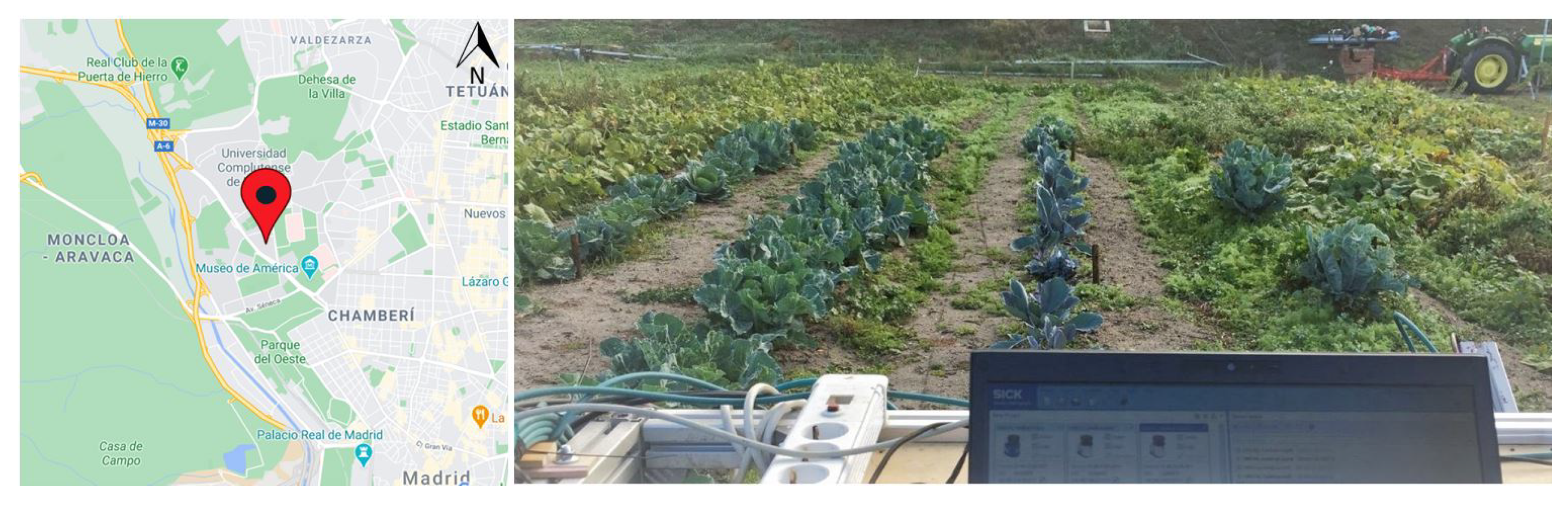
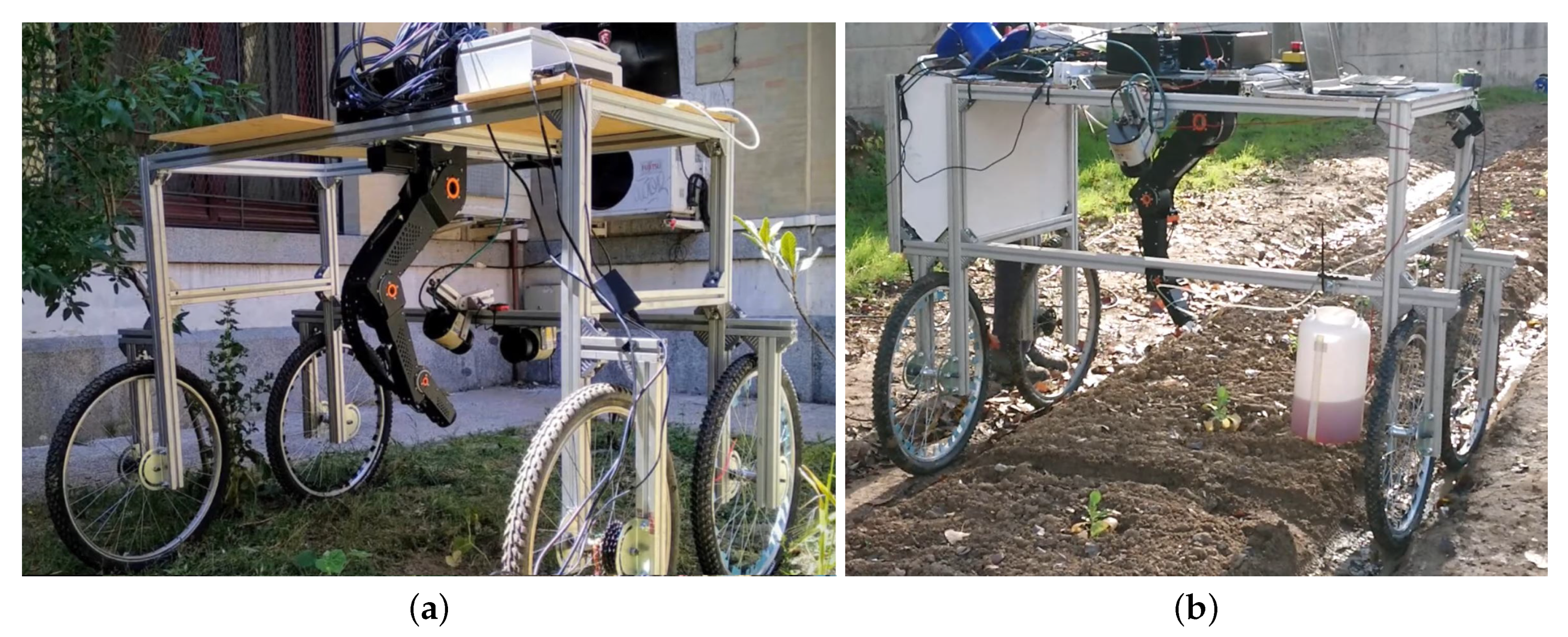
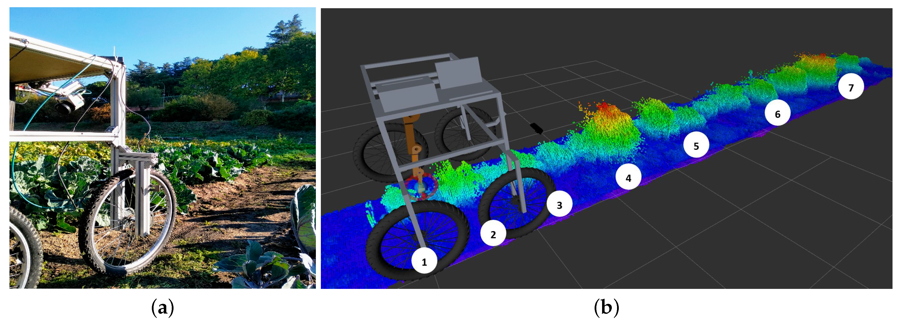
2.1. Materials

To develop this research, experiments were conducted in fields with cabbages in single rows, located at ETSIAAB-UPM ( 40 ° 26′38.9″ N 3 ° 44′19.3″ W), as shown in Figure 1. The crops were planted at the beginning of September 2019, obtaining cabbages with a mean diameter of 50 cm and an average height of 25 cm (Figure 1) at harvest.
The specialised fertilisation tasks were developed using a mobile platform (Figure 2a,b), with general dimensions of 1.6 (length) × 1.5 (height) × 0.8 (width) meters; it was built from aluminum profiles (Bosch Rexroth 45 × 45) and supported the robotic arm (Robolink Igus CPR RL-DC-5 STEP RL-D-RBT-5532S-BF). In Table 1, the sensors and actuators of the mobile platform are detailed.

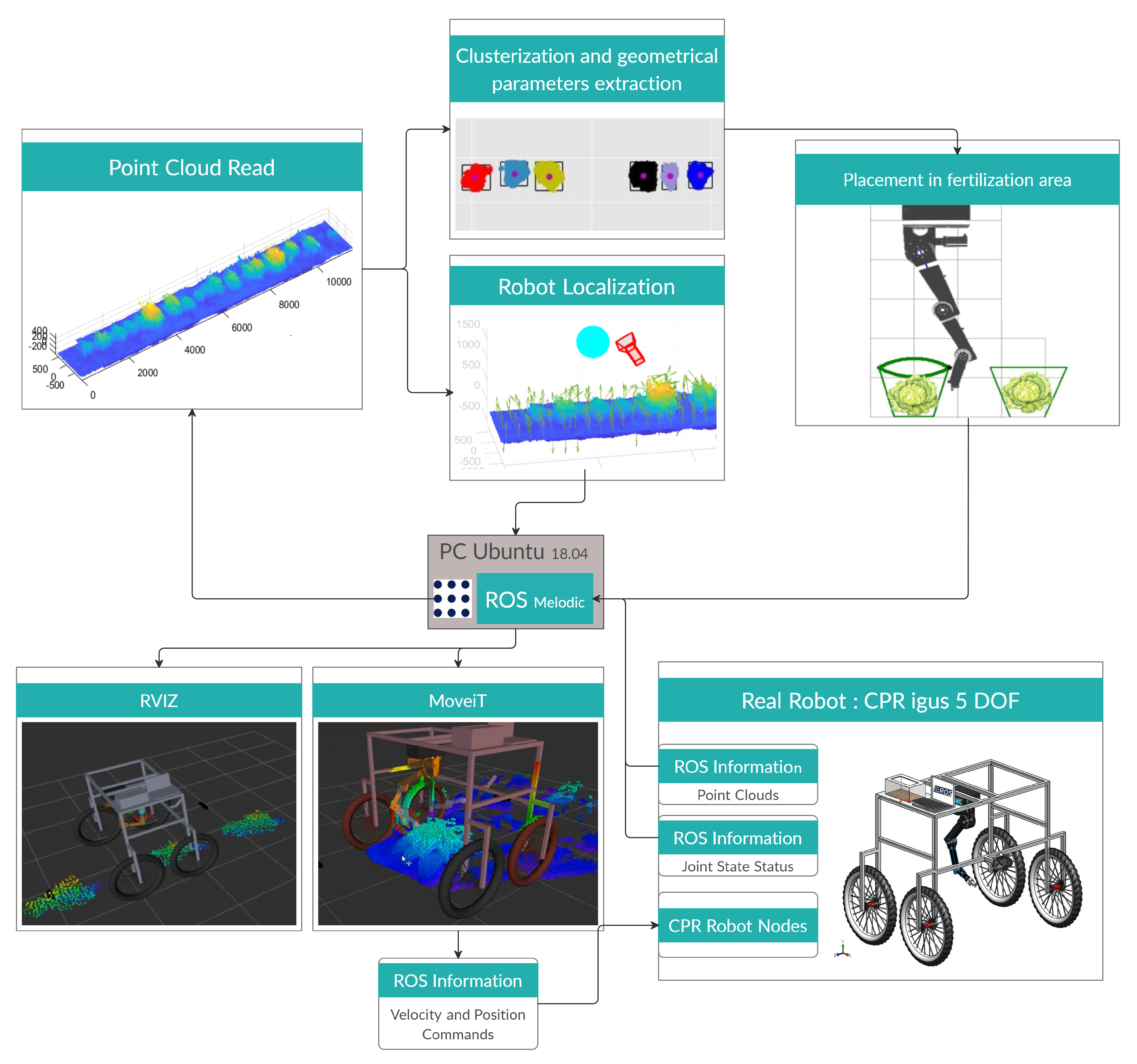
2.2. Interaction between Subsystems

In the information processing and the execution of the robotic fertilisation, several subsystems interact cyclically. The central processing core runs on a computer with Ubuntu 18.04, with ROS (Robot Operating System) Melodic installed. ROS provides a structured communications layer for integrating heterogeneous systems (e.g., sensors, drivers, actuators, etc.) [44]. The use of nodes and topics allowed information exchange between the subsystems as shown schematically in Figure 3, where topics can be regarded as a channel containing the information published by a node. This information can be of different types such as sensor data, joint states, point clouds, etc. [44].
First, three lidars provide point clouds describing the crop row. This information is sent through an ROS topic called “PointCloudRead”, to which the subsystems called “clusterisation and geometrical parameters extraction” and “robot location” both subscribe. The first produces the center coordinates and specific diameters of each plant, while the latter publishes the current relative location within the previously known point cloud directly to a ROS topic. Based on the plant characteristics, the “placement in fertilisation area” subsystem calculates a series of spraying positions taking into account each of the plants’ diameters to cover the entire circumference. These final joint positions are published in a ROS topic used by Moveit to run the collision-free planner to ensure a movement through all prescribed positions without violating any constraints, as e.g., the crop itself or the platforms’ hardware. Finally, this planner generates a sequence of positions and speeds for each of the five arm-motors, transmitted to the robot through a factory owner’s specialised node. To visualize the resulting path in real-time, an interface in Rviz has been implemented to simultaneously see the platform’s position situated within the general crop row point cloud as well as the actuator’s movements.

2.2.1. Data Acquisition and Communications

Prior to the fertilisation stage, the robot and the sensors go over the crop row to take spatial and vegetative measurements of the plants. The obtained point clouds are processed offline to generate the general cloud of the entire crop row (G-PC), as detailed in [43]. The processed cloud is published in a ROS topic “/point_cloud_2”.
The central node is “/move_group”, which receives the current robot joints’ position data, the platform’s position concerning the ground, as well as the real-time status of the detected plant (as point clouds).
Based on the data received, the central node performs the planning of robot’s movements avoiding collisions with the plants. Finally, trajectory and speeds were published in a topic “/move_group/display_planned_path” to move the real robot. The operating frequency of ROS and the system is 10 ms, while the speed of the platform is 1 km/h, so the laser measurements and the commands sent to the robot are processed without delay.

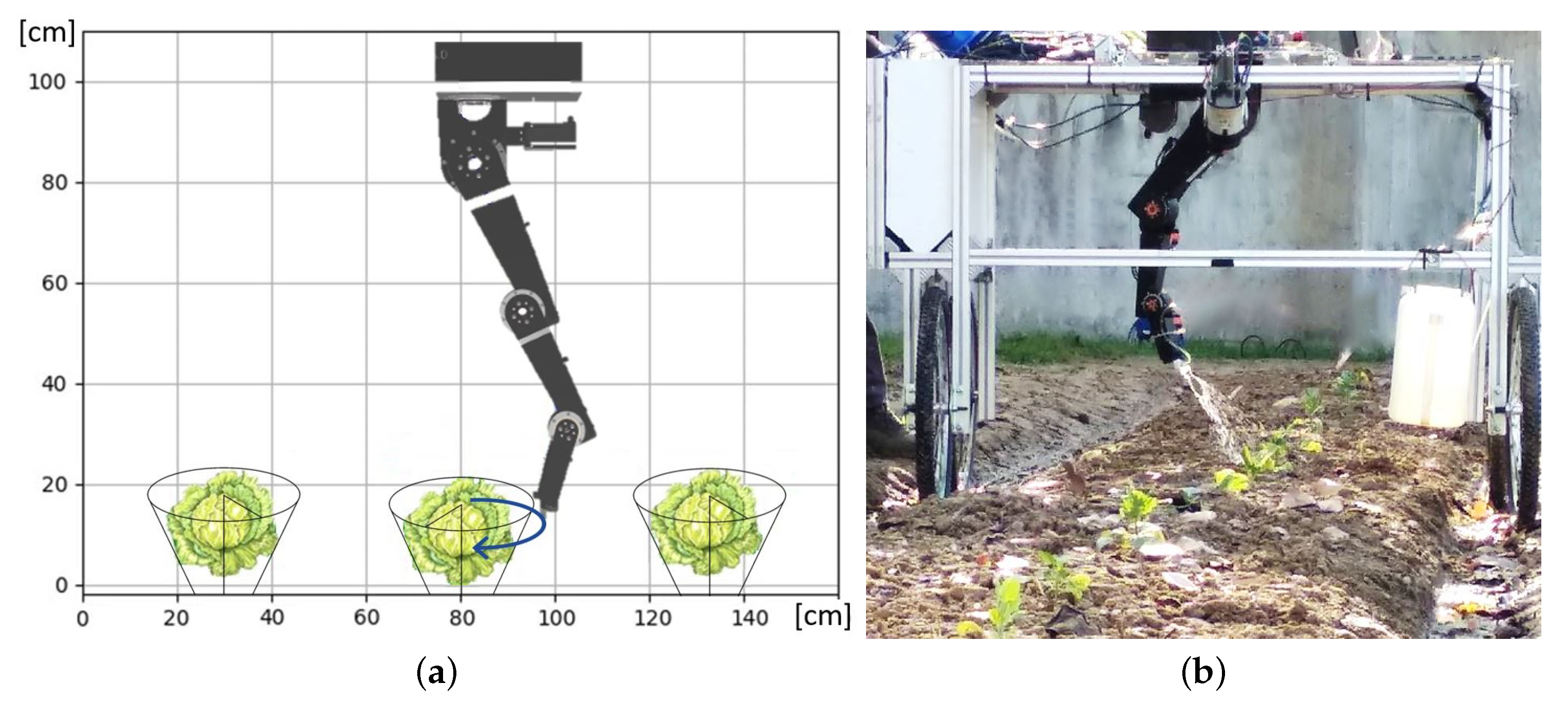
2.2.2. Robot Positioning Based on Geometrical Parameters Extraction of the Plants

As mentioned in Section 2.2, some plant parameters are required to define the fertiliser application zone, in which a semi-circular path can then be marked to apply the fertiliser. In [43], the removal of the soil points from the initial point cloud is discussed, leaving only the crop points. Based on this reduced cloud, the height (h), center (x, y), and plant boundaries are calculated. The edges are enveloped by a cylinder producing a crop radius R. The centers and radii are calculated for each of the plants present in the reduced point cloud as discussed in this section.
Firstly, the reduced point cloud is divided into clusters using the unsupervised learning algorithm K-means, which allows similar group data based on regions [45,46]. This is an iterative method that requires as inputs the data from the unlabeled point cloud and the number k of searched groups. The process starts by randomly assigning the centers [47,48], after which each point is assigned to the nearest centroid based on the Euclidean square distance. For the resulting clusters, the average location of each of the assigned points yields an updated location for the clusters’ centroid. This process is repeated until either the centroids remain unchanged or the change falls below a predefined threshold [49].
Each of the clusters are enveloped by cylinders around the previously mentioned centroids, which defines the maximal plant radius R. These cylinders are subsequently inclined inwards towards the soil to achieve a conical shape. With these geometric parameters, the kinematic positioning of the robot is calculated using the iterative CCD (Cyclic Coordinate Descent) algorithm. Ideally, the position and orientation of the end-actuator should be placed in an exact position with respect to the plant. This relative position depends on the plant’s occupied surface area and height, and could theoretically be outside the robot’s working area, which is why this iterative method [50] is used to approximate the joint positions to cover the area of application of the treatment, while respecting the limitations.
Figure 4a shows an example of the desired positioning for fertilisation, where the plant is enveloped with the conical figure based on the centroids and radius R, defining the inner boundary for the treatment application. This form was found to best encapsulate the experiment plants. Furthermore, the inclination of the cones allows for an inclination of the robot’s final joint.
Figure 4b shows the robot’s positioning based on the described method and the application of the fertiliser jet. The dosage of the fertiliser varies depending on the plant’s geometric characteristics, thus optimising the amount applied. The fertiliser irrigation is developed by activating a solenoid valve and a nozzle attached to the robot’s end.

2.3. Robot Localisation System in Row-Growing

One of the essential aspects during the application of fertiliser with the robotic arm is to locate the robotic platform within the crop at all times. The aspects required for the location include the changing process of the plants’ vegetative state (considering minor variations between one or two days); and the wind’s action.
The proposed method is based on point clouds captured from a set of three lidars placed with their respective positions and orientations concerning the platform. The process is developed for each row, taking the data previously, creating a G-PC and the second cloud L-PC, concerning the sections of G-PC that the platform reads while moving forward (being initially small).
For this development, the “python-PCL” libraries have been used; the point clouds are handled in PCD (Point Cloud Data) format. The proposed algorithm consists of two phases, the first one determines the position by rotation and translation of L-PC over G-PC and the second allows for adjusting the position by extracting key points.
As a preliminary stage, a down-sample is applied to reduce G-PC volume, in order to minimize processing time and optimise computational resources. Additionally, the noise present has been eliminated based on the local density method [51,52], which determines the probability that the point is an outlier, if its value is great [0–1], determining its conservation or elimination based on a threshold.

2.3.1. Normals Calculation

The first stage for the location comprises determining the normals of the surface; based on the primary analysis of the components of the neighboring points, the normals calculation is influenced by the radius and number of points in the neighborhood’s environment. Thus, if the environmental data are insufficient, this calculation will be inaccurate. To calculate the normal vector concerning a point, the normal vector to a plane tangent to the surface of a point is estimated, using the least-squares adjustment. To get the normal vector, the eigenvalues and eigenvectors of the covariance matrix of all the points that make up the area are calculated.
To know the L-PC position in the G-PC, the relative pose is estimated using the rotation and translation of L-PC on G-PC. This method is based on Normal Distribution Transformation, which starts from the previously calculated normals [53,54].

2.3.2. Key Points Extraction

This first stage of the algorithm would be ideal for estimating the robotic platform position. However, it does not contemplate changes or modifications within the environment, so a second stage has been implemented where the key points are calculated to be more robust. For this, the Kdtree type structure is used, which stores a set of k-dimensional points to perform searches between neighbors and establish correspondences between groups of points, adjusting the initial T transformation.
The key points that correspond to the cloud’s relevant characteristics, such as corners or edges, whose environment has enough information and is stable against possible disturbances. The NARF (Normal Aligned Radial Feature) detection method was used, which extracts key points in areas where the underlying surface is stable and the neighboring points contain significant changes; and consider the edges of the objects. Points with high-interest scores are considered key points [55].

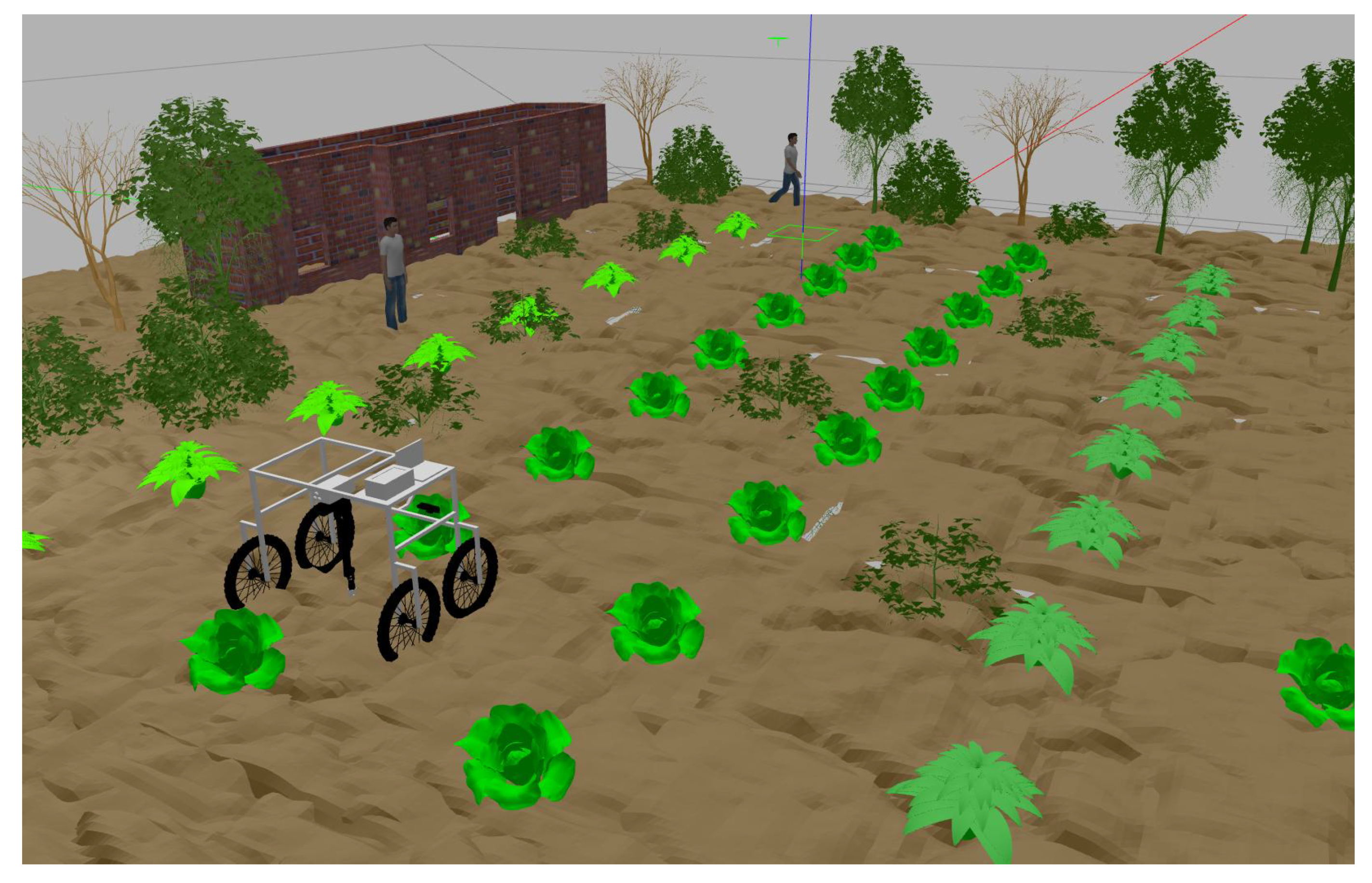
2.4. Simulated Gazebo Environment

To test the algorithms for the robot movement’s execution and its positioning next to the plant before the execution with real data, a simulated world has been developed in Gazebo, which is characterized by its power, realism, and object interaction [56]. The developed environment is shown in Figure 5, replicating the experimental site consisting of extensive vegetation and rows cultivated with different species: cabbages and beans. One of the advantages of using Gazebo is that it allows for simulating various types of environments, including robot models and developments, as well as sensors. The platform model with the robot arm has been incorporated into the simulation. Data taken from Gazebo are very similar to that taken in the physical environment.
A pushbroom lidar is included in the simulation and allows recreation of the point clouds, based on the progress over the crop rows. The laser data are published using ROS topics following the situation in the real environment.
Similarly, the robot joint’s positions are calculated and published in a ROS topic, based on the virtual readings from the simulated environment. In this manner, the planned trajectories and movements can be verified and adjusted where necessary before execution on the real robot. Through the simulated scanning of the virtual crops, the resulting point cloud can be taken into account when calculating the robot’s movements, thereby avoiding collisions with the crops.
The planning and control of movements were developed using ROS’s Moveit tool, which generates the different states for the robot’s joints and the speeds for each state. The fertilisation strategy to only apply to the soil immediately surrounding the plant, taking into account the plant’s geometric characteristics, forms the main objective for this optimisation.
The main benefit of including this pre-testing phase is to ensure that the developed algorithms are compatible with the simulated robot as well as the real robot in their respective environments.

3. Results and Discussion

The results shown below have allowed for verifying the algorithms and procedures described in the methodology. Several tests have been developed using synthetic and real point clouds.

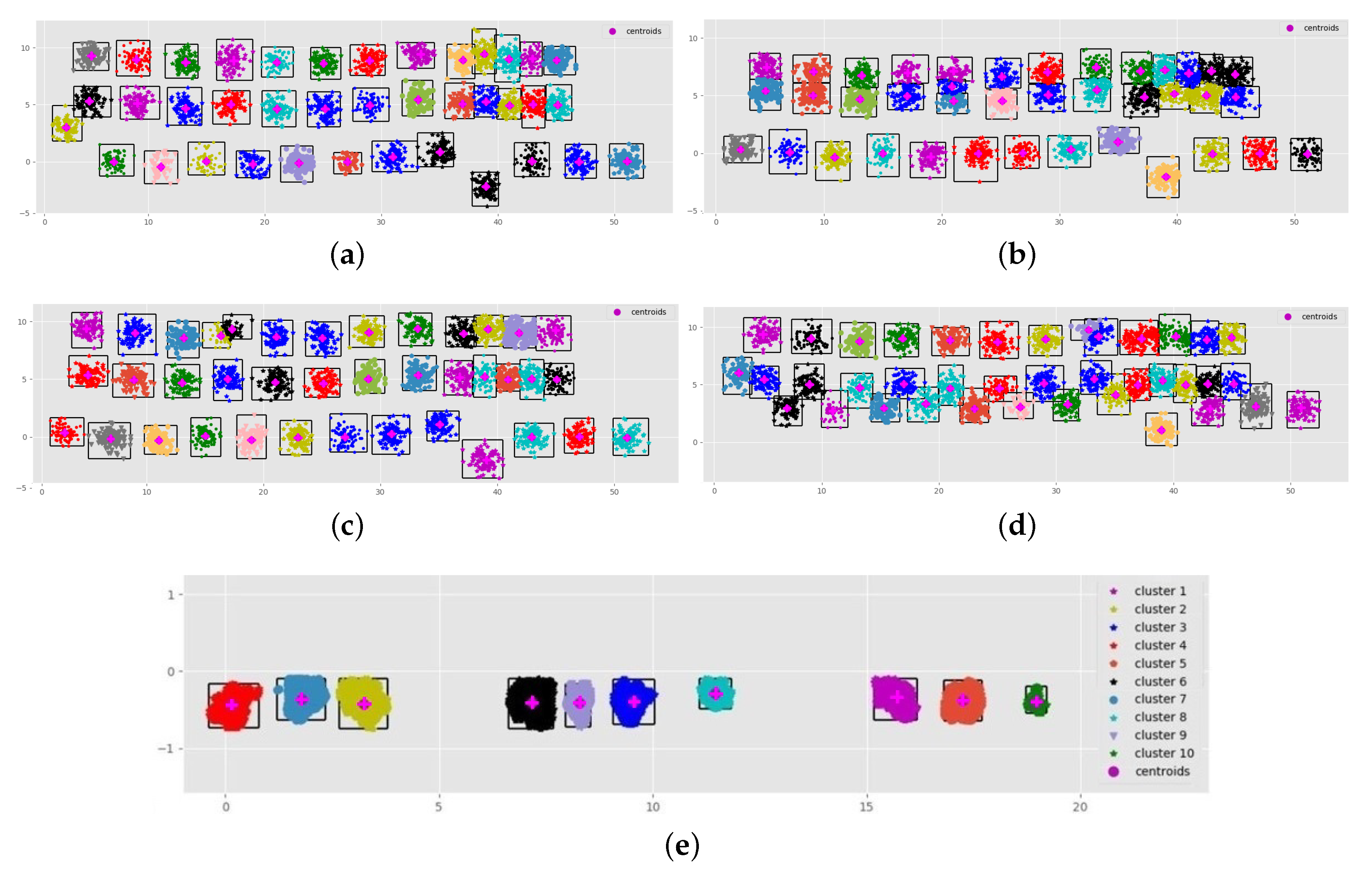
3.1. Geometrical Parameters Extraction from Point Cloud Plants

To verify the geometrical parameters extraction algorithm, tests have been developed with synthetic data and later with real data. In the first instance, (synthetic data) have been obtained from the gazebo environment, generating point clouds of the plants corresponding to the XY plane (ground), to get the clusters, centers and radii. The heights correspond to the cloud data on the z-axis (the maximum values).
The point clouds in Figure 6a–d were acquired from the gazebo environment. For this data generation, 39 plants were placed and distributed by rows as shown in Figure 5, with different spacing variations. As a result, Figure 6a–d shows each cloud’s center with points in fuchsia color, the edges with black quadrilaterals, and each group has been assigned a random color based on the classification to distinct each other.
The classified data concerning the generated data have an incidence of 98.6%, a value that has been measured based on the known labels (when obtained in Gazebo) and compared with the algorithm classification labels. This value is substantial, considering that several plants were placed close to each other to generate different complexity levels for classification.
The data shown in Figure 6e correspond to a row of the plants in Figure 1 (the development before this work [43] that follows the same line of the Sureveg project). As a result, it shows the clustering assigned to each cloud of points, centers, defined edges and color assignment to identify each cluster.
Table 2 shows the data obtained for this point cloud, sent to the arm positioning subsystem, to generate the joint positions and execute the fertilisation. The X values in Table 2 concerning the horizontal distance of the clusters is not growing because the unsupervised learning k-means algorithm used to form the clusters initializes its centres randomly. Therefore, the resulting order of the centres won’t be strictly increasing; However, to send the plant’s geometric characteristics to the robot planner, these are ordered growing. Figure 4 show an example of a robot position based on geometrical parameters.

3.2. Features Extraction from Point Clouds

This section shows the results obtained after applying the algorithms for the robot’s localisation. To develop these tests, real point clouds have been used, obtained in the fields of Figure 1, corresponding to a row with cabbage cultivation and are shown in Figure 7.
The location system is based on two-point clouds; the first called G-PC (Global Point Cloud), previously obtained by making a pass over the row with the platform; it is used as the basis for location. The second L-PC point cloud (Local Point Cloud) is obtained as the platform advances; this second cloud is small at the beginning and increases as the platform advances.

3.2.1. Normals Extraction

The respective normals calculated for each down-sample percentages applied to the original cloud are shown; Figure 7a. 60%, Figure 7b. 40%, Figure 7c. 22%, Figure 7d. 10%. Normals are shown on the original cloud to show the loss of information as the down-sample increases.
Based on the tests performed, the best results were obtained with a reduction of 22% in the volume; in addition, there is no loss of relevant information, and the computational process improves.
As the percentage reduction in the cloud’s volume increases, the number of normals is also reduced (Figure 7a), losing information and making it difficult to locate with great accuracy.

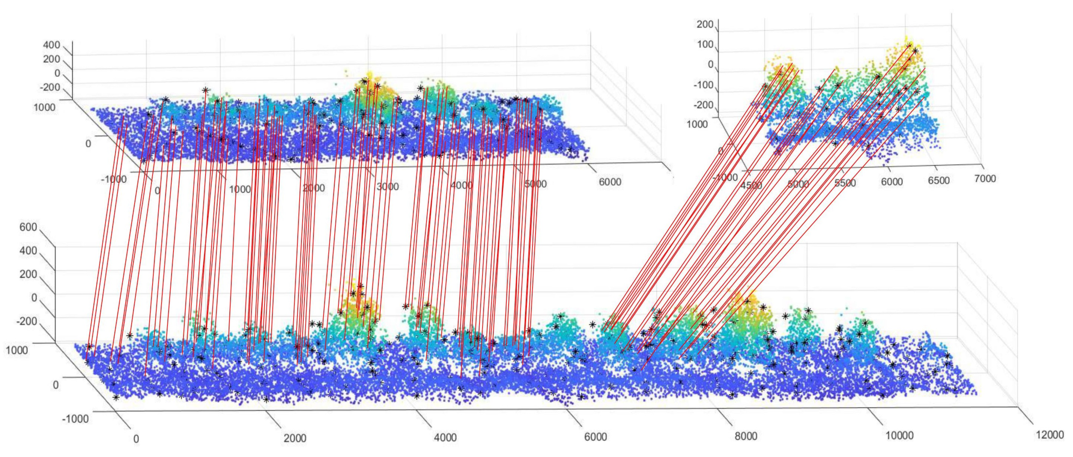
3.2.2. Key Points Extraction and Matching

Figure 8 in the lower part shows the G-PC (with a down-sample applied reducing the volume from 2.361.060 to 524.313), while the upper part corresponds to a first section (L-PC) read by the platform from the beginning of the row towards the middle, and the next cloud (L-PC) corresponds to a part of the row read at a height between 6 and 8 m from the G-PC. The clouds shown have been previously reduced with a down-sample of 22% generating more relevant results.
Key points correspond to corners, edges, or sections that contain enough information; although the environment is slightly changing from one day to the next because of the wind or the slight growth of vegetables, the key points tested in the cloud remain the same areas of the point clouds, according to different tests performed between readings on different days.
In Figure 8, the key points determined by the system can be observed with black asterisks, giving 17,462 key points. The red lines show the correspondence of L-PC points with the points of the G-PC, with a 97.3% efficiency. This allows for getting the position of the local cloud, and thus the position of the robotic platform within the crop, the experiments and measurements carried out are shown in the following section.

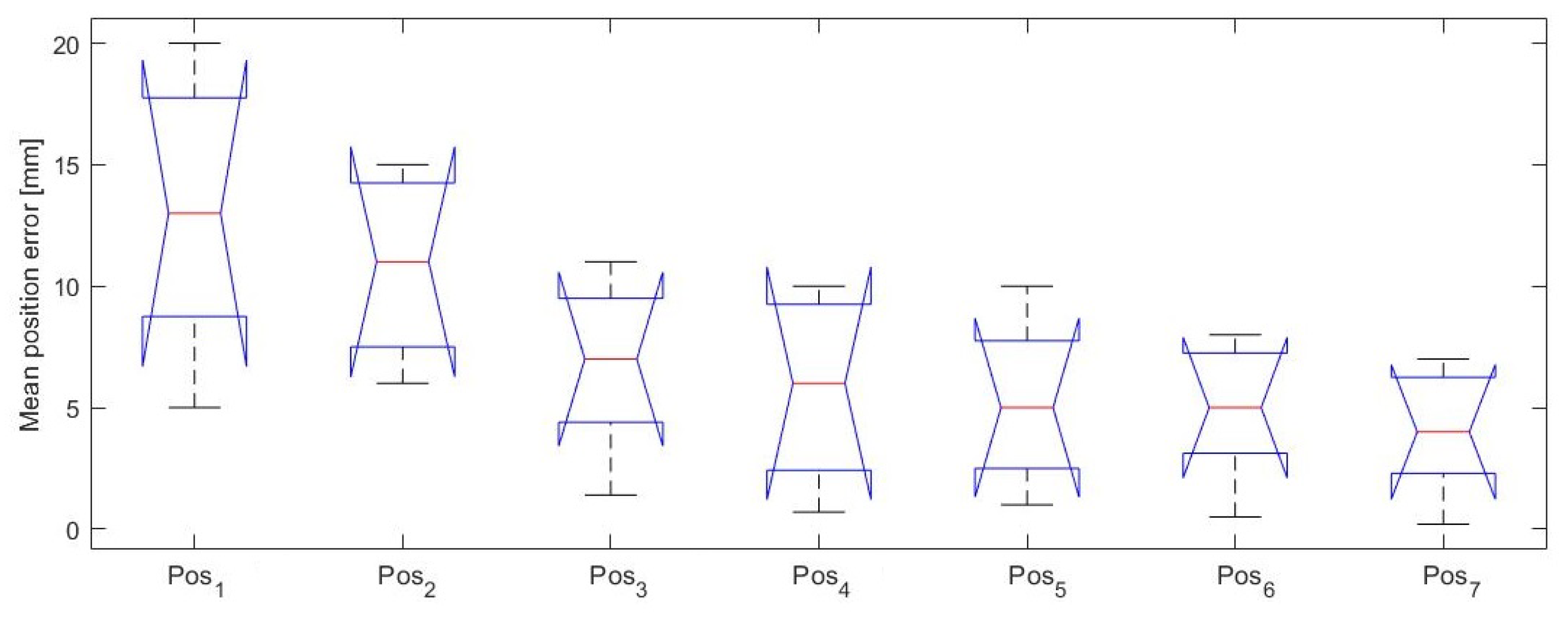
3.3. Localisation Test

Tests performed to estimate the position consisted of taking readings of the point clouds in seven different points of the row separated by a distance of 1.5 m and establishing the location based on the G-PC that contains the cloud of all the row. Figure 9a shows the robotic platform on the row in the test field, while Figure 9b shows the perception system in RVIZ, where the point cloud and the estimated position of the platform are shown for each instance.
As the robotic platform advances from point 1 to points 2, 3, ..., 7, the L-PC accumulates earlier values, which improves the location estimation according to measurements taken. The experiment was repeated ten times showing the following results in Figure 10.
Figure 10 shows the box plot of the data measured in the experiments carried out in Figure 9b. Initially, the average error for positions 1 and 2 ranges between 12 mm; values compared to the full extension of row 1200 mm approximately correspond to 0.1%.
This error does not affect fertilisation because it has been considered a margin of 5 cm additional to the radius defined in the geometrical parameters extraction to encompass the plant and define the passage zone of the robot’s trajectory, thus avoiding the fertiliser being applied on the plant and damaging it.
As the platform progresses, new points are added to the L-PC, allowing for more key points and improved localisation, resulting in errors with an average of 5 mm.
If the robot reaches the end of the row, the local point cloud L-PC is eliminated. The platform turns around and is positioned in the new row. The G-PC is updated (previously captured for each row), and the L-PC begins to be generated again depending on the advance.

4. Conclusions

This article shows the first proof-of-concept of an integrated robotic system for fertilisation using only lidar data to get the plants’ parameters as well as the platform’s relative position. Point clouds allow high precision localisation while at the same time form the basis for the tracking of individual crop growth when recorded over time. To this end, several subsystems were developed and integrated in ROS, alongside a simulation environment in Gazebo, after which the method was executed and validated on a real field test.
The proposed method for localisation through point clouds in strip-cropping environments has demonstrated that the relative location can be reliably established from real-time features’ extraction (in the L-PC) and point cloud matching with a previously established base cloud (G-PC). Low localisation errors were achieved, in the 4 to 13 mm range, allowing to develop with great precision the robotic fertiliser application without affecting the plant.
Applying the geometrical parameters’ extraction subsystem on the G-PC point clouds and the unsupervised learning algorithm K-means allows for identifying clusters concerning each individual plant in the crop row with a high incidence of 98.6%. Furthermore, to extract the clusters’ main characteristics (center, radius, height), trajectory points for the fertilisation movements can be developed for the robotic arm, depending on the plants’ size.
The interaction between the proposed subsystems allows the integral development of fertilisation, exchanging information through ROS nodes and topics. Possible future developments include the use of advanced interfaces for monitoring, and the development of additional tasks such as irrigation, weeding, or picking.

Author Contributions

Conceptualization, A.B., C.V., C.C.U., J.D.C., and A.K.; methodology, A.B. and C.C.U.; software, C.C.U. and A.K.; validation, C.C.U. and A.K.; formal analysis, C.C.U. and A.B.; investigation, C.C.U., A.B., A.K., J.D.C. and C.V.; resources, A.B. and C.V.; data curation, C.C.U. and A.K.; writing—original draft preparation, C.C.U., A.K., J.D.C.; writing—review and editing, C.C.U., A.B., C.V. and A.K.; visualization, A.B. and C.V.; supervision, A.B., J.D.C. and C.V.; project administration, A.B., J.D.C. and C.V.; funding acquisition, A.B. and C.V. All authors have read and agreed to the published version of the manuscript.

Funding

This research has been accomplished within the project “PCI2018-093074 Robot para cultivo en hileras y reciclaje de residuos para producción intensiva de hortalizas y eficiencia energética”, funded by the Ministerio de Ciencia, Innovación y Universidades and the Agencia Estatal de Investigación, within the R+D+i Programa de proyectos Programación conjunta internacional 2018 PCI-2018 and within the project “Sureveg: Strip-cropping and recycling for biodiverse and resource-efficient intensive vegetable production”, within the ERA-net CORE Organic Cofund action: http://projects.au.dk/coreorganiccofund/. Also financial support han been obtain from the project RoboCity2030-DIH-CM, Madrid Robotics Digital Innovation Hub, S2018/NMT-4331, funded by “Programas de Actividades I+D en la Comunidad de Madrid”.

Acknowledgments

This work was accomplished thanks to the important support of: ERAnet CORE Organic Cofound—Sureveg Project, AEI (Agencia Estatal de Investigación), CSIC (Consejo Superior de Investigaciones Científicas), Centro de Automática y Robótica—Departamento de Ingeniería Agroforestal, ETSI Agronómica, Alimentaria y de Biosistemas—Universidad Politécnica de Madrid. Special appreciation is given for the contribution made by Juan José Ramírez and Pablo Guillén Colomer during the development of field tests.

Conflicts of Interest

The authors declare no conflict of interest.

Abbreviations

The following abbreviations are used in this manuscript:
L-PCLocal Point Cloud
PCLPoint Cloud Library
G-PCGeneral Point Cloud
ROSRobot Operating System
RVIZROS Visualization

Appendix A

Link to Sureveg Concept project: https://www.youtube.com/watch?v=s60mOl1v7cA&t=5s.

References

  1. Cranfield, J.A.L. Framing consumer food demand responses in a viral pandemic. Can. J. Agric. Econ. Can. D’agroeconomie 2020, 68, 151–156. [Google Scholar] [CrossRef]
  2. Ritson, C. Population Growth and Global Food Supplies. In Food Education and Food Technology in School Curricula: International Perspectives; Springer International Publishing: Cham, Switzerland, 2020; pp. 261–271. [Google Scholar]
  3. Pachapur, P.K.; Pachapur, V.L.; Brar, S.K.; Galvez, R.; Le Bihan, Y.; Surampalli, R.Y. Food Security and Sustainability. In Sustainability; John Wiley & Sons, Ltd.: Hoboken, NJ, USA, 2020; Chapter 17; pp. 357–374. [Google Scholar]
  4. Srivasta, R.K. Influence of Sustainable Agricultural Practices on Healthy Food Cultivation. In Environmental Biotechnology Vol. 2; Springer International Publishing: Cham, Switzerland, 2020; pp. 95–124. [Google Scholar]
  5. Rendon, P.; Steinhoff-Knopp, B.; Saggau, P.; Burkhard, B. Assessment of the relationships between agroecosystem condition and soil erosion regulating ecosystem service in Northern Germany. bioRxiv 2020. [Google Scholar] [CrossRef]
  6. Silva, V.; Yang, X.; Fleskens, L.; Ritsema, C.; Geissen, V. Soil contamination by pesticide residues—what and how much should we expect to find in EU agricultural soils based on pesticide recommended uses? Sci. Total Environ. 2019, 653, 1532–1545. [Google Scholar] [CrossRef]
  7. Fernandes, C.L.F.; Volcão, L.M.; Ramires, P.F.; Moura, R.R.D.; Da Silva Júnior, F.M.R. Distribution of pesticides in agricultural and urban soils of Brazil: A critical review. Environ. Sci. Process. Impacts 2020, 22, 256–270. [Google Scholar] [CrossRef] [PubMed]
  8. Tarla, D.N.; Erickson, L.E.; Hettiarachchi, G.M.; Amadi, S.I.; Galkaduwa, M.; Davis, L.C.; Nurzhanova, A.; Pidlisnyuk, V. Phytoremediation and Bioremediation of Pesticide-Contaminated Soil. Appl. Sci. 2020, 10, 1217. [Google Scholar] [CrossRef] [Green Version]
  9. Majoro, F.; Wali, U.G.; Munyaneza, O.; Naramabuye, F.X.; Mukamwambali, C. On-site and Off-site Effects of Soil Erosion: Causal Analysis and Remedial Measures in Agricultural Land—A Review. Rwanda J. Eng. Sci. Technol. Environ. 2020, 3. [Google Scholar] [CrossRef]
  10. Asociación Española Agricultura de Conservación Suelos Vivos. Situación Actual de la Agricultura de Conservación en España. Available online: https://www.interempresas.net/Agricola/Articulos/126980-Situacion-actual-de-la-agricultura-de-conservacion-en-Espana.html (accessed on 27 August 2020).
  11. Loures, L.; Chamizo, A.; Ferreira, P.; Loures, A.; Castanho, R.; Panagopoulos, T. Assessing the Effectiveness of Precision Agriculture Management Systems in Mediterranean Small Farms. Sustainability 2020, 12, 3765. [Google Scholar] [CrossRef]
  12. Poblete-Echeverría, C.; Fuentes, S. Editorial: Special Issue “Emerging Sensor Technology in Agriculture”. Sensors 2020, 20, 3827. [Google Scholar] [CrossRef]
  13. Singh, R.K.; Aernouts, M.; De Meyer, M.; Weyn, M.; Berkvens, R. Leveraging LoRaWAN Technology for Precision Agriculture in Greenhouses. Sensors 2020, 20, 1827. [Google Scholar] [CrossRef] [Green Version]
  14. Cubero, S.; Marco-Noales, E.; Aleixos, N.; Barbé, S.; Blasco, J. RobHortic: A Field Robot to Detect Pests and Diseases in Horticultural Crops by Proximal Sensing. Agriculture 2020, 10, 276. [Google Scholar] [CrossRef]
  15. Moysiadis, V.; Tsolakis, N.; Katikaridis, D.; Sørensen, C.G.; Pearson, S.; Bochtis, D. Mobile Robotics in Agricultural Operations: A Narrative Review on Planning Aspects. Appl. Sci. 2020, 10, 3453. [Google Scholar] [CrossRef]
  16. Fue, K.G.; Porter, W.M.; Barnes, E.M.; Rains, G.C. An Extensive Review of Mobile Agricultural Robotics for Field Operations: Focus on Cotton Harvesting. AgriEngineering 2020, 2, 150–174. [Google Scholar] [CrossRef] [Green Version]
  17. Hussain, M.; Naqvi, S.H.A.; Khan, S.H.; Farhan, M. An Intelligent Autonomous Robotic System for Precision Farming. In Proceedings of the 2020 3rd International Conference on Intelligent Autonomous Systems (ICoIAS), Singapore, 26–29 February 2020; pp. 133–139. [Google Scholar]
  18. Cofund, C.O. Sureveg Project. Available online: https://projects.au.dk/coreorganiccofund/core-organic-cofund-projects/sureveg/ (accessed on 27 August 2020).
  19. Hernández-Pajares, M.; Moreno-Borràs, D. Real-Time Detection, Location, and Measurement of Geoeffective Stellar Flares From Global Navigation Satellite System Data: New Technique and Case Studies. Space Weather 2020, 18, e2020SW002441. [Google Scholar] [CrossRef] [Green Version]
  20. Pradhan, C.; Mohapatra, K.K.; Saren, S. GPS based sampling for determination of fertility status of some villages of Jatani block of khordha district, Odisha. IJCS 2020, 8, 2980–2984. [Google Scholar] [CrossRef]
  21. Kulkarni, A.A.; Dhanush, P.; Chetan, B.S.; Gowda, C.S.T.; Shrivastava, P.K. Applications of Automation and Robotics in Agriculture Industries A Review. IOP Conf. Ser. Mater. Sci. Eng. 2020, 748, 012002. [Google Scholar] [CrossRef]
  22. Sharifi, M.; Meenken, E.; Hall, B.; Espig, M.; Finlay-Smits, S.; Wheeler, D. Importance of Measurement and Data Uncertainty in a Digitally Enabled Agriculture System. In Nutrient Management in Farmed Landscapes; Farmed Landscapes Research Centre, Massey University: Palmerston North, New Zealand, 2020. [Google Scholar]
  23. Zhang, Q.; Li, S.; Xu, Z.; Niu, X. Velocity-Based Optimization-Based Alignment (VBOBA) of Low-End MEMS IMU/GNSS for Low Dynamic Applications. IEEE Sens. J. 2020, 20, 5527–5539. [Google Scholar] [CrossRef]
  24. Miletiev, R.; Kapanakov, P.; Iontchev, E.; Yordanov, R. High sampling rate IMU with dual band GNSS receiver. In Proceedings of the 2020 43rd International Spring Seminar on Electronics Technology (ISSE), Demanovska Valley, Slovakia, 13–17 May 2020; pp. 1–5. [Google Scholar]
  25. Fu, L.; Gao, F.; Wu, J.; Li, R.; Karkee, M.; Zhang, Q. Application of consumer RGB-D cameras for fruit detection and localization in field: A critical review. Comput. Electron. Agric. 2020, 177, 105687. [Google Scholar] [CrossRef]
  26. Singh, P.; Kaur, A.; Nayyar, A. Role of Internet of Things and image processing for the development of agriculture robots. In Swarm Intelligence for Resource Management in Internet of Things; Elsevier: Amsterdam, The Netherlands, 2020; pp. 147–167. [Google Scholar]
  27. Zong, Z.; Liu, G.; Zhao, S. Real-Time Localization Approach for Maize Cores at Seedling Stage Based on Machine Vision. Agronomy 2020, 10, 470. [Google Scholar] [CrossRef] [Green Version]
  28. Aghi, D.; Mazzia, V.; Chiaberge, M. Local Motion Planner for Autonomous Navigation in Vineyards with a RGB-D Camera-Based Algorithm and Deep Learning Synergy. Machines 2020, 8, 27. [Google Scholar] [CrossRef]
  29. Fariña, B.; Toledo, J.; Estevez, J.I.; Acosta, L. Improving Robot Localization Using Doppler-Based Variable Sensor Covariance Calculation. Sensors 2020, 20, 2287. [Google Scholar] [CrossRef] [Green Version]
  30. Zhao, D.; Whittaker, W. High Precision In-Pipe Robot Localization with Reciprocal Sensor Fusion. arXiv 2020, arXiv:2002.12408. [Google Scholar]
  31. Szaj, W.; Pieniazek, J. Vehicle localization using laser scanner. In Proceedings of the 2020 IEEE 7th International Workshop on Metrology for AeroSpace (MetroAeroSpace), Pisa, Italy, 22 June–5 July 2020; pp. 588–593. [Google Scholar]
  32. Vora, A.; Agarwal, S.; Pandey, G.; McBride, J. Aerial Imagery based LIDAR Localization for Autonomous Vehicles. arXiv 2020, arXiv:2003.11192. [Google Scholar]
  33. de Miguel, M.Á.; García, F.; Armingol, J.M. Improved LiDAR Probabilistic Localization for Autonomous Vehicles Using GNSS. Sensors 2020, 20, 3145. [Google Scholar] [CrossRef] [PubMed]
  34. Wang, Z.; Shen, Y.; Cai, B.; Saleem, M.T. A Brief Review on Loop Closure Detection with 3D Point Cloud. In Proceedings of the 2019 IEEE International Conference on Real-time Computing and Robotics (RCAR), Irkutsk, Russia, 4–9 August 2019; pp. 929–934. [Google Scholar]
  35. Comba, L.; Biglia, A.; Ricauda Aimonino, D.; Gay, P. Unsupervised detection of vineyards by 3D point-cloud UAV photogrammetry for precision agriculture. Comput. Electron. Agric. 2018, 155, 84–95. [Google Scholar] [CrossRef]
  36. Fu, W.; Liu, R.; Wang, H.; Ali, R.; He, Y.; Cao, Z.; Qin, Z. A Method of Multiple Dynamic Objects Identification and Localization Based on Laser and RFID. Sensors 2020, 20, 3948. [Google Scholar] [CrossRef] [PubMed]
  37. Liu, J.; Hoover, R.C.; McGough, J.S. Mobile Fiducial-Based Collaborative Localization and Mapping (CLAM). In Proceedings of the USCToMM Symposium on Mechanical Systems and Robotics, Rapid City, SD, USA, 14–16 May 2020; pp. 196–205. [Google Scholar]
  38. Yu, H.; Zhen, W.; Yang, W.; Scherer, S. Line-based 2D-3D Registration and Camera Localization in Structured Environments. IEEE Trans. Instrum. Meas. 2020, 69, 8962–8972. [Google Scholar] [CrossRef]
  39. Alves, R.C.; de Morais, J.S.; Yamanaka, K. Cost-effective Indoor Localization for Autonomous Robots using Kinect and WiFi Sensors. Intel. Artif. 2020, 23, 33–55. [Google Scholar]
  40. Barnes, E.; Moran, M.; Pinter, P., Jr.; Clarke, T. Multispectral remote sensing and site-specific agriculture: Examples of current technology and future possibilities. In Proceedings of the Third International Conference on Precision Agriculture, Minneapolis, MN, USA, 23–26 May 1996; pp. 845–854. [Google Scholar]
  41. Huang, Y.; Thomson, S.J.; Lan, Y.; Maas, S.J. Multispectral imaging systems for airborne remote sensing to support agricultural production management. Int. J. Agric. Biol. Eng. 2010, 3, 50–62. [Google Scholar]
  42. Cardim Ferreira Lima, M.; Krus, A.; Valero, C.; Barrientos, A.; Del Cerro, J.; Roldán-Gómez, J.J. Monitoring Plant Status and Fertilization Strategy through Multispectral Images. Sensors 2020, 20, 435. [Google Scholar] [CrossRef] [Green Version]
  43. Krus, A.; van Apeldoorn, D.; Montoro, J.J.R.; Ubierna, C.V. Acquiring plant features with optical sensing devices in an organic strip-cropping system. In Proceedings of the 12th European Conference on Precision Agriculture, Técnicas Avanzadas en Agroalimentación LPF-TAGRALIA, Montpellier, France, 8–11 July 2019; Volume 1, pp. 104–105. [Google Scholar]
  44. Quigley, M.; Conley, K.; Gerkey, B.; Faust, J.; Foote, T.; Leibs, J.; Wheeler, R.; Ng, A.Y. ROS: An open-source Robot Operating System. In Proceedings of the ICRA Workshop on Open Source Software, Kobe, Japan, 12–17 May 2009; Volume 3, p. 5. [Google Scholar]
  45. Pham, D.; Otri, S.; Afify, A.; Mahmuddin, M.; Al-Jabbouli, H. Data clustering using the bees algorithm. In Proceedings of the 40th CIRP International Manufacturing Systems Seminar, Liverpool, UK, 30 May–1 June 2007. [Google Scholar]
  46. Qi, J.; Yu, Y.; Wang, L.; Liu, J.; Wang, Y. An effective and efficient hierarchical K-means clustering algorithm. Int. J. Distrib. Sens. Netw. 2017, 13, 1550147717728627. [Google Scholar] [CrossRef] [Green Version]
  47. Ding, C.; He, X. K-Means Clustering via Principal Component Analysis. In Proceedings of the Twenty-First, International Conference on Machine Learning, ICML ’04, Banff, AB, Canada, 4–8 July 2004; Association for Computing Machinery: New York, NY, USA, 2004; p. 29. [Google Scholar]
  48. El Agha, M.; Ashour, W.M. Efficient and fast initialization algorithm for k-means clustering. Effic. Fast Initial. Algorithm K-Means Clust. 2012, 4, 21–31. [Google Scholar] [CrossRef]
  49. Scarlatache, F.; Grigoraş, G.; Chicco, G.; Cârţină, G. Using k-means clustering method in determination of the optimal placement of distributed generation sources in electrical distribution systems. In Proceedings of the 2012 13th International Conference on Optimization of Electrical and Electronic Equipment (OPTIM), Brasov, Romania, 24–26 May 2012; pp. 953–958. [Google Scholar]
  50. Martin, A.; Barrientos, A.; del Cerro, J. The natural-CCD algorithm, a novel method to solve the inverse kinematics of hyper-redundant and soft robots. Soft Robot. 2018, 5, 242–257. [Google Scholar] [CrossRef] [PubMed]
  51. Ning, X.; Li, F.; Tian, G.; Wang, Y. An efficient outlier removal method for scattered point cloud data. PLoS ONE 2018, 13, e0201280. [Google Scholar] [CrossRef] [PubMed] [Green Version]
  52. Rusu, R.; Blodow, N.; Marton, Z.; Soos, A.; Beetz, M. Towards 3D Object Maps for Autonomous Household Robots. In Proceedings of the IEEE/RSJ International Conference on Intelligent Robots and Systems, San Diego, CA, USA, 29 October–2 November 2007; pp. 3191–3198. [Google Scholar]
  53. Shi, X.; Peng, J.; Li, J.; Yan, P.; Gong, H. The Iterative Closest Point Registration Algorithm Based on the Normal Distribution Transformation. Procedia Comput. Sci. 2019, 147, 181–190. [Google Scholar] [CrossRef]
  54. Magnusson, M.; Duckett, T. A comparison of 3D registration algorithms for autonomous underground mining vehicles. In Proceedings of the European Conference on Mobile Robotics (ECMR 2005, Italy), Ancona, Italy, 7–10 September 2005; pp. 86–91. [Google Scholar]
  55. Hänsch, R.; Weber, T.; Hellwich, O. Comparison of 3D interest point detectors and descriptors for point cloud fusion. ISPRS Ann. Photogramm. Remote Sens. Spat. Inf. Sci. 2014, 2, 57. [Google Scholar] [CrossRef] [Green Version]
  56. Buyuksalih, I.; Bayburt, S.; Buyuksalih, G.; Baskaraca, A.; Karim, H.; Rahman, A.A. 3D Modelling and Visualization Based on the Unity Game Engine–Advantages and Challenges. ISPRS Ann. Photogramm. Remote Sens. Spat. Inf. Sci. 2017, 4, 161. [Google Scholar] [CrossRef] [Green Version]
Figure 1. Test fields with single cabbage rows. Source: Author.
Agronomy 11 00011 g001
Figure 2. Structure with the robot arm positioned in the center of the platform. (a) mobile platform assembled, (b) robotic platform—on field. Source: Author.
Agronomy 11 00011 g002
Figure 3. Layout of subsystems connection: data acquisition, clusterisation and geometrical parameters extraction, placement in fertilisation area, localisation and motion planning. Source: Author.
Agronomy 11 00011 g003
Figure 4. Positioning strategy for fertiliser application based on geometrical parameters. (a) Geometric description of robot positioning and movement, (b) fertiliser application by robotic arm. Source: Author.
Agronomy 11 00011 g004
Figure 5. Simulated environment of strip-cropping field developed in Gazebo for algorithm tests. Source: Author.
Agronomy 11 00011 g005
Figure 6. K-means classification and geometrical parameters extraction from synthetic and real data. (a) Synthetic data from 39 point clouds (distribution 1), (b) synthetic data from 39 point clouds (distribution 2), (c) synthetic data from 39 point clouds (distribution 3), (d) synthetic data from 39 point clouds (distribution 4), (e) real data from row cultivation. Source: Author.
Agronomy 11 00011 g006
Figure 7. Normals calculated from G-PC with different down-sample levels applied, (a) 60%, (b) 40%, (c) 22%, (d) 10%, represented on the original point cloud (G-PC). Source: Author.
Agronomy 11 00011 g007
Figure 8. Matching correspondences between key points from L-PC (upper—two captured partial sections) to G-PC(lower). Source: Author.
Agronomy 11 00011 g008
Figure 9. Test execution and data visualization for localisation. (a) Mobile robotic platform—on field, (b) mobile robotics platform position and data visualization in rviz. Source: Authors.
Agronomy 11 00011 g009
Figure 10. Box diagram for measured location positions taken in Figure 9b. Source: Author.
Agronomy 11 00011 g010
Table 1. Elements and components of the mobile platform.
ElementAmountDescription
Robot Igus CPR 5 DOF1Actuator
Lidar (SICK AG)32D Laser sensor
Parrot Sequoia1Multi-spectral camera
User interface1ROS Central Core
Control box1Electrical system
Table 2. Centers, radios and height obtained from Figure 6e.
Cluster12345678910
Radio (cm)51534953515554424839
X pos (cm)161038092020172074024011908101850
Y pos (cm)−39−51−41−40−38−39−37−30−39−36
Height (cm)40413944424544394140
Publisher’s Note: MDPI stays neutral with regard to jurisdictional claims in published maps and institutional affiliations.

