Mobile Plant Disease Classifier, Trained with a Small Number of Images by the End User

Abstract

Mobile applications that can be used for the training and classification of plant diseases are described in this paper. Professional agronomists can select the species and their diseases that are supported by the developed tool and follow an automatic training procedure using a small number of indicative photographs. The employed classification method is based on features that represent distinct aspects of the sick plant such as, for example, the color level distribution in the regions of interest. These features are extracted from photographs that display a plant part such as a leaf or a fruit. Multiple reference ranges are determined for each feature during training. When a new photograph is analyzed, its feature values are compared with the reference ranges, and different grades are assigned depending on whether a feature value falls within a range or not. The new photograph is classified as the disease with the highest grade. Ten tomato diseases are used as a case study, and the applications are trained with 40–100 segmented and normalized photographs for each disease. An accuracy between 93.4% and 96.1% is experimentally measured in this case. An additional dataset of pear disease photographs that are not segmented or normalized is also tested with an average accuracy of 95%.

1. Introduction

The economic and ecological overhead of crop management can be significantly increased if plant diseases are not detected and treated early. Larger amounts of pesticides are required if a disease has already spread, and part of the production may be permanently lost. The plants need to be continuously monitored in order for the initial disease symptoms to be recognized. Medium and small producers may not be able to afford to hire professional agronomists for long periods. Several precision agriculture and Internet of Things (IoT) tools have recently been proposed that can assist producers in efficiently monitoring the health of their plants. Although most of these tools cannot provide a certified diagnosis, they can guide the producer to perform additional, more reliable tests [1], if it is necessary, to verify a disease infection. The diagnosis of a plant disease can be based on its symptoms: under- or over-development of tissues or necrosis or alternation in the appearance of plant parts. The progression of the primary or secondary symptoms depends on biotic agents. Similar symptoms may also be caused by the use of herbicides, chemicals and air pollution.

Some approaches require advanced tools and hardware or a combination of information derived from multiple sources (e.g., sensors) to perform a reliable plant disease diagnosis. Image processing can be combined with sensor indications, meteorological data and information entered by the producers in response to questionnaires. Unmanned Air Vehicles (UAVs) and Internet of Things (IoT) sensors mounted in constant positions or on robots/tractors can be used to monitor large crops. A review of Machine Learning (ML) techniques for the detection of biotic stress in crops can be found in [2]. Ballesteros et al. discussed several UAV-assisted approaches in [3]. IoT sensors, robotics and image processing exploited by Convolutional Neural Networks (CNN) were combined in [4] for plant disease diagnosis. Natural language processing was applied in [5] for crop pests and disease recognition. A review of machine vision approaches used in the identification of common invertebrates (butterflies, snails, etc.) in crops was discussed in [6]. A review of deep learning techniques applied in hyperspectral information can be found in [7,8].

Many approaches combine image processing with deep learning techniques to detect plant diseases. We are especially interested in the tomato and pear diseases that are used as case studies in this paper. Grape leaf diseases were diagnosed in [9] by combining various CNN architectures (AlexNet, ResNet, GoogLeNet) and Support Vector Machines (SVM). Pear and apple fruit classes were examined in [10], where MobileNet and MobileNetV2 deep learning architectures for mobile devices were compared. Key influencing factors and severity recognition of pear diseases using deep learning were examined in [11]. Three pear diseases with six levels of severity were discriminated. A CNN was used in [12] to detect if a leaf is infected by one of the 12 tomato and potato diseases supported. In [13], an efficient smart mobile application model that is based on MobileNet CNN was used to recognize 10 tomato leaf diseases. A CNN architecture that recognizes 10 tomato leaf diseases was presented in [14] and was compared with Inception V3, Mobilenet and VGG16. The size of the trained model in [14] required 1.69 MB. Seven tomato disease classes were tested in [15] by AlexNet and VGG16 in order to investigate how accuracy and speed are affected by the number of training images and other parameters such as minibatch size, weight and bias learning rate. In [16], transfer learning was employed for use on mobile devices at reduced cost using pre-trained EfficientNetB0, MobileNetV2 and VGG 19 models as feature extractors. The resulting model size ranged between 24 MB and 155 MB.

Mobile applications, such as the ones presented in this paper, are also of special interest. A survey on mobile applications for various smart agriculture tasks can be found in [17]. Fertilizer and irrigation control was performed by the mobile application described in [18]. A review on mobile applications for plant disease signature detection was presented in [19]. Image processing and neural network architectures perform poorly on mobile devices due to limited resources (memory, processing speed) [20]. In the simplest case, mobile devices can be used for plant disease diagnosis based on descriptions entered by the end user in text format [21]. The referenced approaches in this category require internet connection and are often based on decision trees that model the combinations that should be examined according to the declared symptoms. A more advanced approach based on text analysis was presented in [22]. In this approach, an Android application was developed, addressing more than 100 crop disease problems of cotton/wheat leaves/fruits based on fuzzy inference. A mobile application for maize diseases was discussed in [23]. Another mobile application with a user-friendly interface that performs fungal disease detection was presented in [24]. The diagnosis was assisted by meteorological historic data and a chat with the end user. The mobile application presented in [25] estimated the damage caused by the Tuta absoluta pest. A mobile CNN approach for the diagnosis of 26 diseases from 14 crop species was presented in [26].

Deep-learning-based plant disease classification applications can achieve a superior accuracy that is often higher than 95%. However, these approaches require a large number of training samples and a long training period. The size ratio of the training dataset to test dataset is usually higher than 3:1. These training difficulties also exist in other machine learning techniques such as SVM. The training process in these approaches cannot be performed by an end user, e.g., an agronomist or a cultivator. The list of supported diseases and species can be extended only by the developer of these applications. For this reason, the plant disease applications presented in the literature support either a limited set of popular plant diseases (tomatoes, potatoes, citrus, grapevines, etc.) or they are developed for specific plants and lack portability. Many referenced plant disease applications use trained models several megabytes in size, and mobile platforms may not be able to provide the necessary resources. The work presented in this paper concerns two mobile applications (Disease Classification Trainer, Disease Classifier) that can be used to train and classify new diseases based on a method that does not require a large training dataset. Agronomists can exploit these tools to customize the supported set of diseases and perform appropriate training that satisfies the accuracy goals set. The complexity of the employed method is low, and the resulting diagnosis rules are stored in a file that is a few kilobytes in size. Therefore, this implementation is appropriate for mobile applications. Classification is performed almost instantaneously, while the training latency depends only on the time needed for the interactive selection of the training photographs.

An RGB photograph displaying a sick plant part (e.g., leaf or fruit) is segmented into four Regions of Interest (ROIs): the background, the normal part, the spots and the halo around the spots. Most of the features extracted concern histogram features for each ROI color. The ranges of these histograms form the disease signature. In real-time operation, the extracted feature values are compared to the feature ranges stored in each disease signature, and a grade is estimated that is used to sort the diseases. An initial version of this classification method was presented in [27] in the framework of the Plant Disease application. This method can also be used for different image classification applications such as skin disorder recognition [28]. The experimental results presented in this paper show that, despite the simplicity and extendibility of the proposed classification method, high accuracy (>95%) can be achieved in the recognition of some diseases even if a relatively small portion of the dataset is used for training. The applications were developed using the Visual Studio 2019—Xamarin platform sourced from the official Microsoft webpage, and, thus, they can be deployed as Android, iOS or Windows applications (Universal Windows Platform—UWP).

The approach presented in this paper differs from our previous work in the following ways: (a) the classification mobile application is extended to support dynamic training and loading of disease recognition rules, (b) a training application is developed to automate the training procedure on new diseases, (c) the classification algorithm is extended to support the comparison of a feature value with multiple ranges (only two ranges were supported in [27]) to improve accuracy, (d) the results presented in this work concern the classification of a larger number of diseases (10 tomato leaf diseases are examined in one case study instead of the five citrus diseases tested in [27]) and (e) a dataset of four pear diseases is also tested to measure the accuracy of the proposed method using photographs that are not segmented or normalized. The tomato photographs tested in this paper were retrieved from publically available datasets, while the ones displaying pear leaves are a private collection retrieved from the region of Achaia, Greece.

The dataset, the classification algorithm and the developed mobile applications are described in Section 2. The experimental results are presented in Section 3, and discussion follows in Section 4.

2. Materials and Methods

2.1. Dataset and Supported Diseases

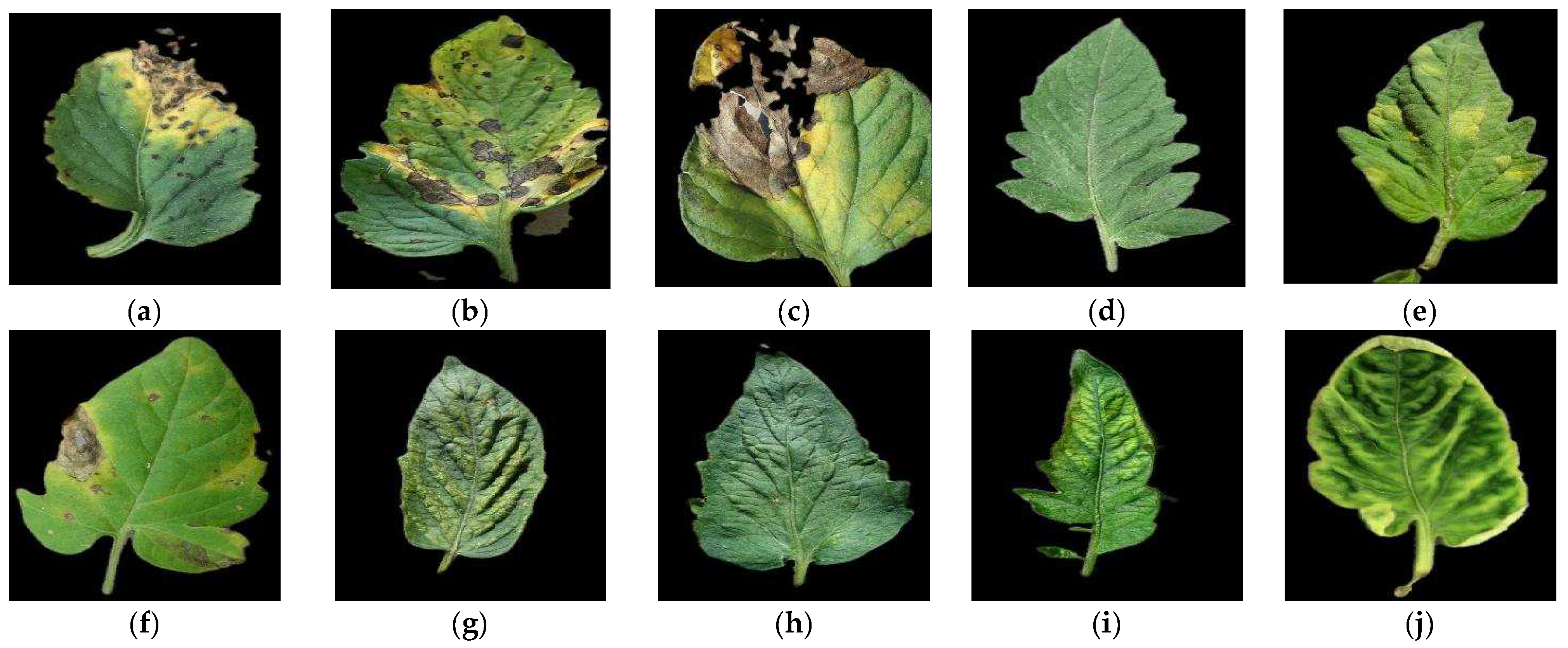
The tomato disease dataset used in this work was retrieved from PlantVillage [29]. In this dataset, 50,000 photographs are offered concerning 38 common plant diseases of potatoes, tomatoes, corn, pepper, apple, strawberries, etc. The photographs are available in three formats: (a) color scale, (b) gray scale and (c) color and segmented. Other datasets that can be exploited by our applications are the RoCoLe, containing annotated coffee leaf images [30], and the LeLePhid [31], with images of lemon leaves infected by aphid insects. We used the color and segmented tomato disease photographs from PlantVillage where the background is black. The background segmentation can be performed by our classification application if the plant part has a different color than the background, e.g., yellow citrus fruits or red tomatoes with green leaf or brown soil background or if the sick plant part is placed on a white sheet or bench. Employing a more sophisticated background separation method is part of our future work. Our application also supports normalization methods, such as dynamic range extension, that are described in detail in [27]. We randomly selected 140 photographs of each one of the 10 tomato diseases that are available in PlantVillage: healthy, bacterial spot, early/late blight, leaf mold, septoria, spider mites, target spot, mosaic and yellow leaf curl virus. In this way, a dataset of 1400 photographs was created. This is a far larger dataset compared to the one used in [27], where 22–56 photographs were used for each one of the five citrus diseases. All the photographs from the PlantVillage dataset are in JPEG format with 256 × 256 pixel resolution. Indicative photographs for each one of the supported diseases are shown in Figure 1.

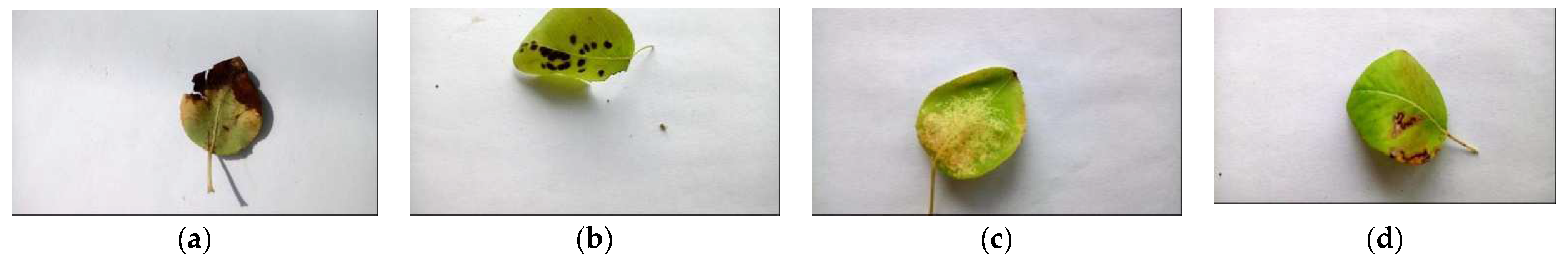
A pear dataset populated with photographs that are neither segmented or normalized was also used. This dataset is unbalanced since different numbers of photographs per disease are available. Four pear diseases are displayed: fire blight (120 images), fuzicladium fungi (80 images), podosphaera powdery mildew (82 images) and septoria fungi (40 images). These photographs display pear leaves retrieved from the Achaia county of Greece. The sizes of these photographs are not identical and are approximately 550 × 310 pixels. A public dataset of pear diseases was not employed because we required a leaf to be placed on a white sheet or marble bench in order for the system to separate the background using color thresholds. Indicative photographs for the 4 pear diseases examined in this paper are shown in Figure 2.

2.2. Image Processing and Classification

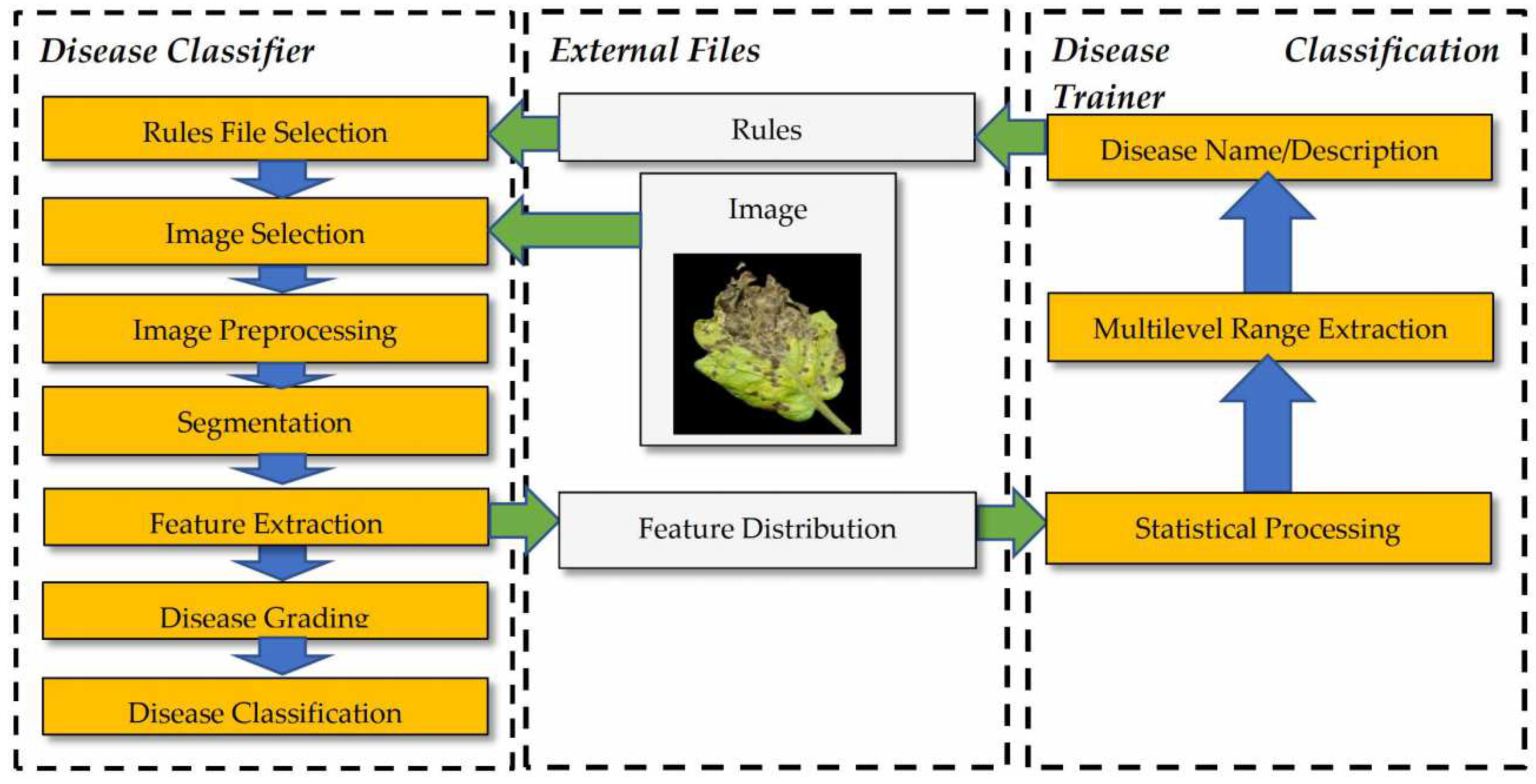
In this paragraph, a brief introduction to the image processing and classification techniques employed in [27] is presented, emphasizing to the new features offered by the Disease Classifier application. The steps followed in the pair of applications that were developed are shown in Figure 3. The information exchanged between the Disease Classifier and the Disease Classification Trainer is structured as a pair of files: (a) the Ranges file, containing the limits of each feature as determined after analyzing all the training photographs of a disease in the Disease Classifier application, and (b) the Rules file, generated after statistically processing the Ranges file in the Disease Classification Trainer application.

Initially, the disease recognition Rules file is selected in the Disease Classification application. A default pre-trained Rules file can also be selected if the training on the desired diseases has not yet been performed. The format of a Rules file is described in the following paragraphs. This option did not exist in the initial version of Plant Disease [27] application, where the rules were hardcoded, and any modification required a project rebuild in the Visual Studio 2019 Xamarin platform sourced from the original Microsoft webpage. An image is selected as a next step. The images display a sick part of the plant, e.g., a leaf or a fruit, and the background should be either dark or white for easier separation. During image preprocessing, a normalization in various color scales (RGB, Hue–Saturation–Lightness (HSL), Hue–Saturation–Value (HSV) or L*a*b format) can be performed, as described in [32]. The default color of the images is used in this work, since the first dataset with tomato diseases was already normalized. The photographs in the second dataset with pear diseases were inherently not normalized, while the normalization facilities offered by the Disease Classifier were not employed in order to treat the testing of this dataset as a worst case scenario.

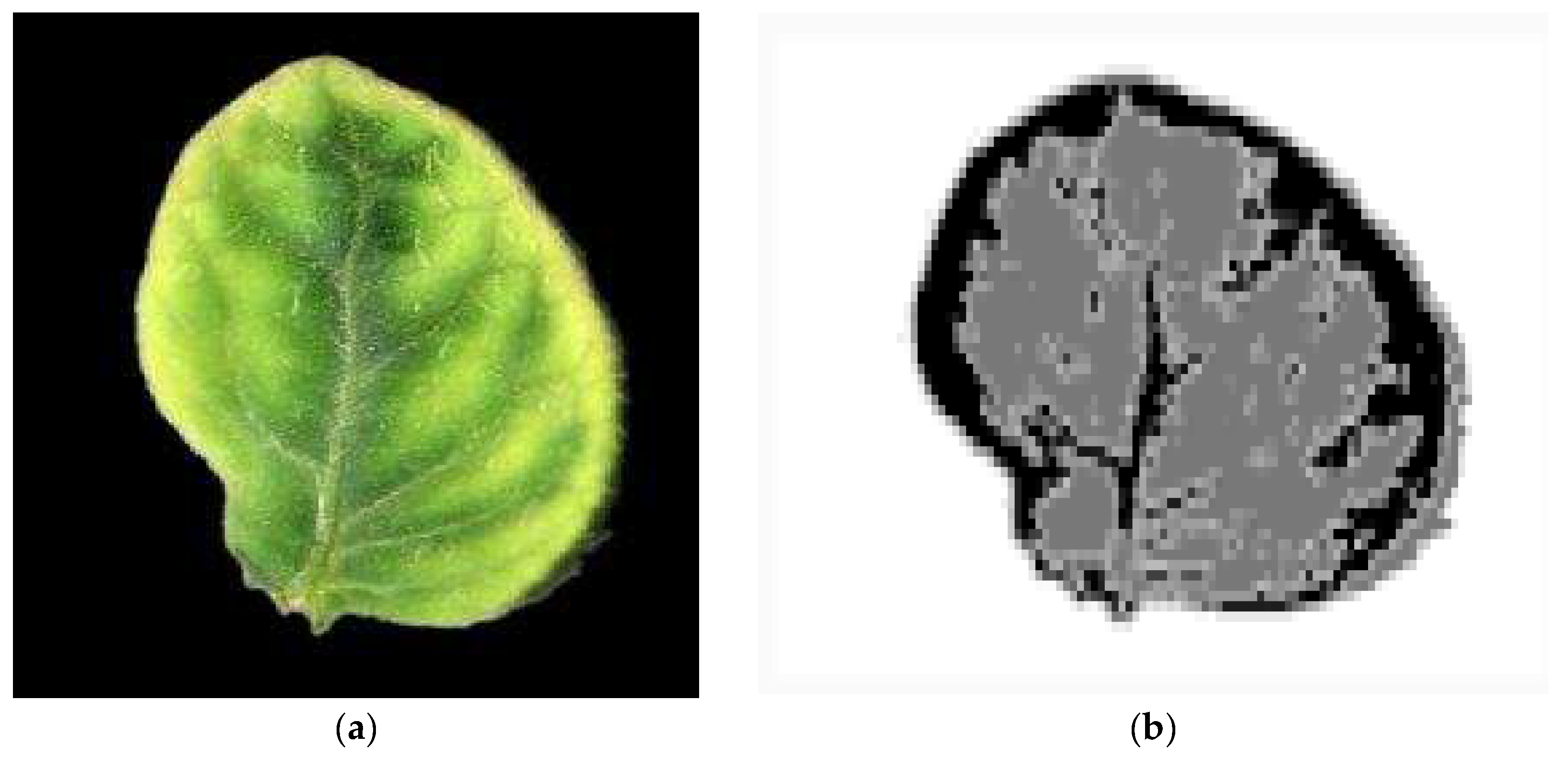
As a next step, the image is segmented in the four ROIs, the background (ignored), the normal leaf, the spots and the halo around the spots, based on two triplets of thresholds. An example image segmentation is shown in Figure 4. It is assumed that the yellow leaf regions are the spots. The background, normal leaf and spots are displayed in white, gray and black, respectively. A halo zone of 5 pixels is defined around the spots, and it is displayed in a lighter gray color. One threshold triplet (Tb) is used to separate the background and one (Ts) for the lesion spots. The image is scanned once, and the pixel color is compared to the Tb threshold triplet. Pixels that do not belong to the background are initially marked as normal leaf. Then, the color of the pixels belonging to the normal leaf ROI is compared to the Ts that separates the lesion spots. If the spots are darker than the normal leaf, the pixels with color below Ts are marked as spots. The adjacent spot islands are merged and then all the spot islands are numbered to identify the total number of spots. More details of this process can be found in [27]. The halo is defined as a zone of specific width around each spot. Very small spots can be considered as noise and ignored.

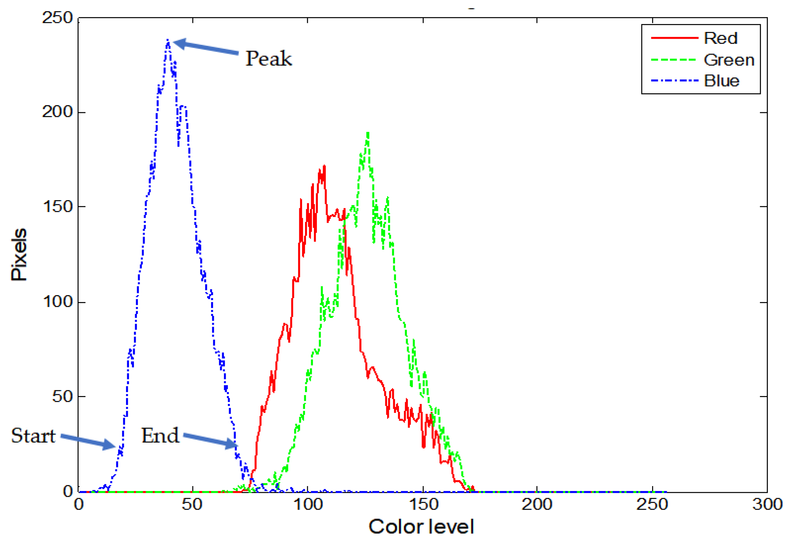
Histograms are constructed for each one of the red, green and blue colors of the pixels belonging to each one of the three ROIs (normal, spot, halo). Histograms for the red, green and blue color of a normal leaf ROI, reconstructed in Matlab, are shown in Figure 5. The horizontal axis displays the color level (0 to 255). The value of each point in a histogram curve is the number of pixels in the specific ROI that have the corresponding color level. More specifically, the hist[256] is the vector of values (initially all 0s) of a histogram that corresponds to a specific color (e.g., red) and ROI. For each pixel in this ROI that is found with red color equal to r, hist[r] is increased by 1. As can be seen in Figure 5, each one of the histograms consists of a single lobe. It is expected that the histograms corresponding to the same disease, color and ROI will be similar. However, instead of trying to measure the similarity between a pair of histograms following a complicated method, we simply compare the start, end and peak of the lobes. The start and the end points of the lobe can be selected as the lobe curve points that cross a specific level (e.g., 10% of the peak value). The majority of features used in the classification process are the start, the end and the peak values of the various histograms. The full list of the employed features used for classification are shown in

Table 1. The features used by the classification process.

Feature	Notes
Number of spots	A spot is defined as an island of adjacent pixels
Area of the spots	(lesion spot pixels)/(overall plant part pixels)
Average gray level of the spots	The average gray level extracted from the pixels belonging in each one of the normal, spot and halo ROIs
Average gray level of the normal plant part
Average gray level of the halo
Histogram lobe start, peak, end	3 ROIs × 3 colors × 3 parameters = 27 features
Average moisture	The average daily moisture, minimum and maximum daily temperatures estimated for a number of dates determined by the user (not tested in this paper)
Average minimum temperature
Average maximum temperature

[27].

The number of spots is estimated by finding the number of spot islands (adjacent spot pixels). The area of the spots can be a fraction between 1% and 100%. The weather features displayed in Table 1 (moisture, temperature) were not taken into consideration in the present work. After feature extraction, the disease grading takes place, and the supported diseases are sorted based on the grade they received. The current photograph is classified as the disease with the highest grade.

In this work, the extracted features can be buffered and their limits stored in the Rules csv file. In this way, training on new diseases can be performed automatically by a non-expert in computer science, e.g., an end user such as an agronomist. Using some indicative training photographs from each disease, the agronomist can start the Disease Classifier application, and the extracted features of a training photograph can be appended to the Range file of the specific disease. All the Ranges files are loaded to the Disease Classification Trainer application that performs a statistical processing in order to define the reference ranges. Moreover, two strings are defined in the trainer: the name of the disease and the message that should be displayed in the classification results. This message can be a short description of the actions that have to be taken by the producer. Alternatively, this message can be a link to a webpage where detailed instructions can be given to the producer in order to treat the diagnosed disease.

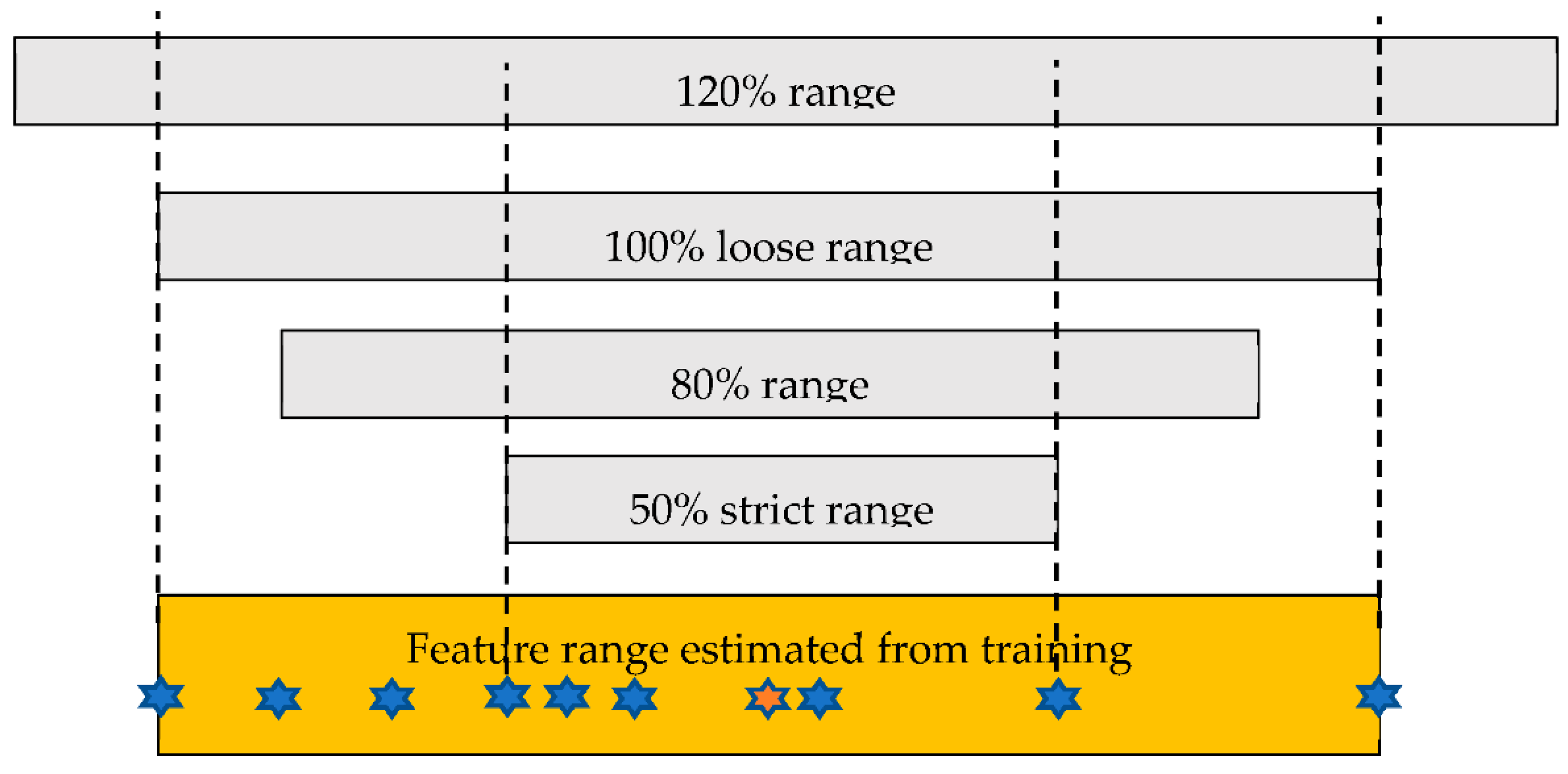
The statistical processing performed in the Disease Classification Trainer determines the ranges of each feature from the values appended in the Range file produced by the Disease Classifier (see Figure 3). The minimum and maximum values of each feature, as they appear in the training photographs, are characterized as the “loose range”, as can be seen in Figure 6. All 10 stars in the orange strip correspond to the training values of a specific feature. The loose range is determined by the minimum (the star at the far left) and the maximum (the star at the far right). A “strict range” is defined by a fraction a of the training values of this feature as follows: The median value is initially located within the loose range. Then, a% of the training values that are closer to the median is used to define the strict range, as shown in Figure 6. The red star is the median. If a = 0.5, then the five training values that are closer to the median are found in order to define the strict range, which is actually 50% of the loose range (the strict range is defined from the minimum and the maximum of these 5 values). The strict and loose range limits (4 values) of each feature in a disease are stored in the Rules file by the Disease Classification Trainer application when the training is completed, along with the disease name and message. Other ranges (e.g., 80% or 120%) can be defined in reference to the 100% loose range in real time within the Disease Classification application. Please note that, in the original Plant Disease application [27], only a strict range and a loose range were used, both of which were defined in a different way: the strict range was what is now called a loose range (100%), and the loose range was defined by extending the strict range by an arbitrary offset (e.g., 10).

The classification method followed in the present work was based on grading each disease by comparing the feature values extracted from a new image with the ranges defined in the Rules file. A weight is added to the grade if the feature value is found within a specific range. For example, if a weight of 10 is assigned to each one of the four ranges displayed in Figure 6, then, if a feature value falls within the 80%, 100% and 120% but not in the 50% range, a grade equal to 30 is given for this feature for the specific disease. The grades of all features are added. The grade G_d of a disease d can be formally defined as follows:

$$G\left(F_{id}\right)={\displaystyle \sum }_{r=1}^R{x}_{ird}{G}_{ird},$$

(1)

$$x_{ird}=1 if F_{ird\_L}\le F_{id}\le F_{ird\_H}, 0 \mathrm{otherwise}$$

(2)

$$G_d={\displaystyle \sum }_{i=1}^{F_N}G\left(F_{id}\right),$$

(3)

The parameter F_N is the number of features (32 in our case), R is the number of ranges defined and G_ird is the grade given if the feature value i is found within range r for the disease d. The overall grade for the feature i in the disease d is the G(F_id) estimated in Equation (1). The binary parameter x_ird is 1 if the feature value F_id is found within range r or is 0 otherwise. The disease grading method employed in [27] is the one described in Equations (1)–(3) for R = 2. The analyzed image is classified as the disease with the highest grade.

2.3. Description of the Developed Applications

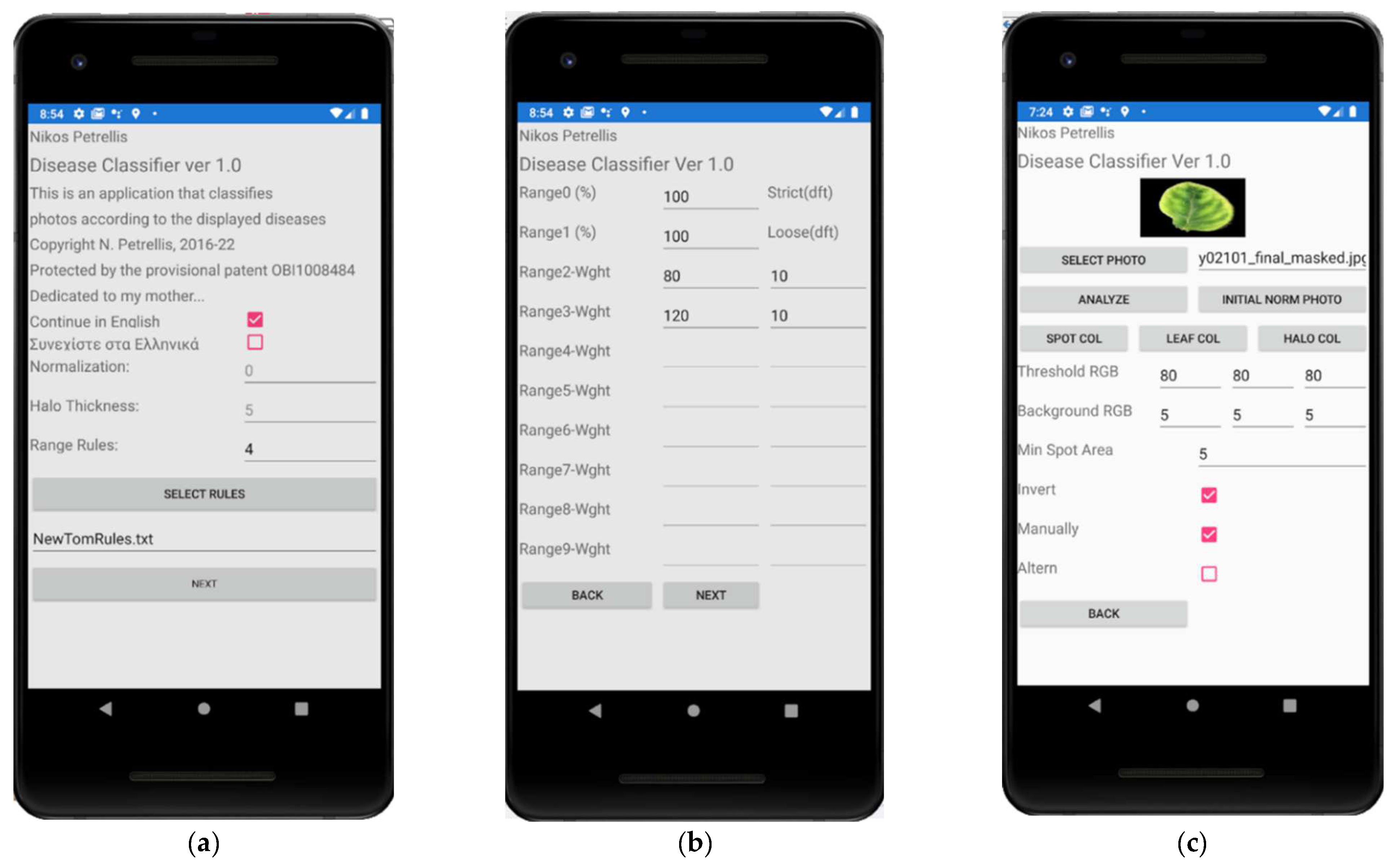
The pages of the Disease Classifier application appear in Figure 7. On the introductory page (Figure 7a), the user can define the language of the interface, a color normalization type (0 stands for no normalization), the thickness of the halo in pixels (default: 5 pixels) and the number of ranges R (default: 2). If there is no halo in the spots of a plant disease, the halo thickness, and the weights of the halo features can be set to 0. The button “Select Rules” can be used to load a Rules file that contains the definition of a disease and its feature ranges. The name of the file appears below this button (NewTomRules.txt). If the “Range Rules” field is set to a number higher than 2, then the page shown in Figure 7b appears. Up to 10 ranges can be defined in the current version. The default strict and loose ranges defined, as described in Section 2.2, cannot be modified. Two fields need to be filled for each one of the extra ranges that are defined: the range percentage (e.g., 80% and 120% for Range 2 and Range 3, respectively) and the weight G given for these ranges during disease grading. More customized weights per disease and feature can be defined by modifying the Rules file with a text editor. The next page is the one shown in Figure 7c–e. On this page, the user selects the image and performs the segmentation through the button “Analyze”, according to the defined threshold triplets (“Threshold RGB”, “Background RGB”).

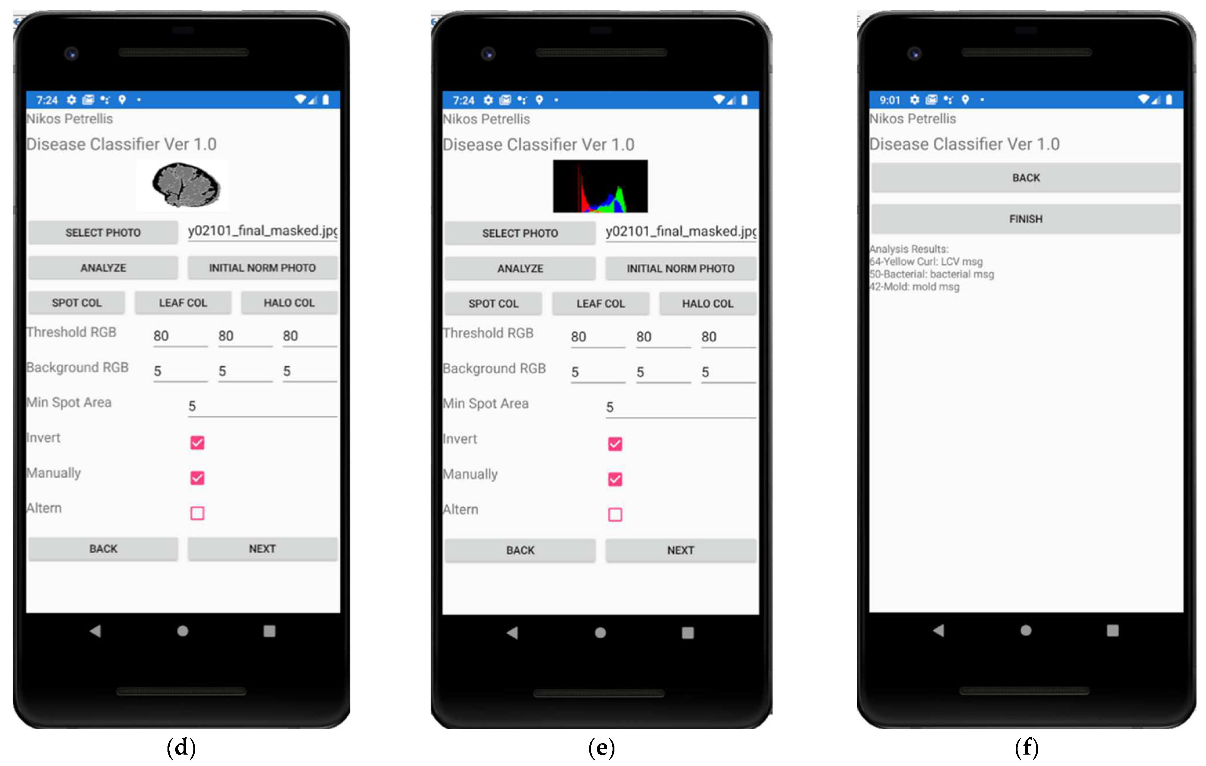
Since the tomato photographs tested in this work have a black background, a pixel is assumed to belong to the background if its R, G, B colors are lower than the “Background RGB” threshold triplet Tb. Similarly, if the background is white, as with the pear diseases, the pixels are assigned to it if the R, G, B values are greater than the triplet Tb. If the spots in a disease are darker than the normal leaf, a pixel that does not belong to the background is assumed to belong to a spot if its R, G, B colors are lower than the corresponding “Threshold RGB” triplet Ts. If the spots are brighter than the normal leaf, the user has to tick the “Invert” check box. In this case, a pixel belongs to a spot if its R, G, B colors are higher than Ts. The “Min Spot Area” field defines the minimum number of pixels a spot requires. Spots with fewer pixels than the “Min Spot Area” are treated as noise and are ignored. The user can assess the quality of the segmentation interactively by bringing back the initial photograph after segmentation using the “Initial Norm Photo” button. However, in this case, the photograph is not displayed in its original form but in its normalized form (in case a normalization method has been enabled in the application). The user can also preview the histograms created after the segmentation, as shown in Figure 7e. The results are shown as displayed in Figure 7f. The top 3 diseases with the higher grade are listed on each line, starting with the grade, the name of the disease and the message that gives instructions to the end user. Additional pages in the Disease Classifier application can be visited to access weather data, but they are not presented in this paper since meteorological data have not been taken into consideration.

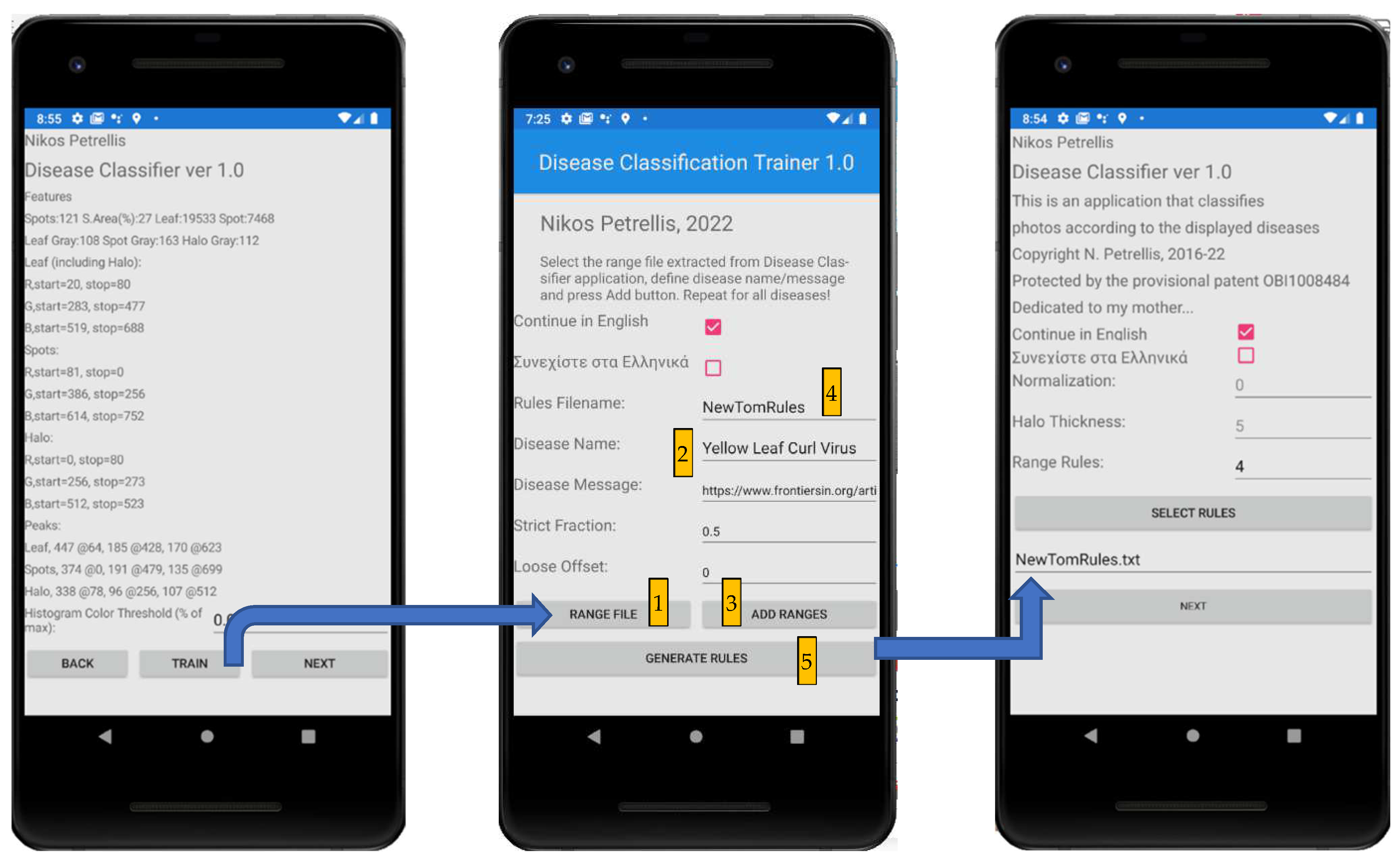
The only page of the Disease Classification Trainer is shown in the middle of Figure 8. In this figure, the entry page and the one with the extracted feature values of the Disease Classifier are also shown in order to explain how training can take place. When a training photograph is selected and analyzed in the Disease Classifier page, as seen in Figure 7c–e, the next page that appears is the one on the left of Figure 8. The user (e.g., an agronomist) can append the extracted feature values to a “Range File” by clicking the “Train” button. When the features from all the training photographs have been appended in different Range files for each disease, these files can be loaded one by one from the Disease Classification Trainer following the sequence shown in the middle of Figure 8. Each Range file is selected (by clicking the “Range File” button), and the name of the corresponding disease is defined, as well as the message that should be displayed. Then, the contents of the Range file are loaded and statistically processed by clicking the “Add Range” button. These three steps are repeated for all the supported diseases. The name of the Rules file is defined next, and the “Generate Rules” button is clicked to store the new Rules file.

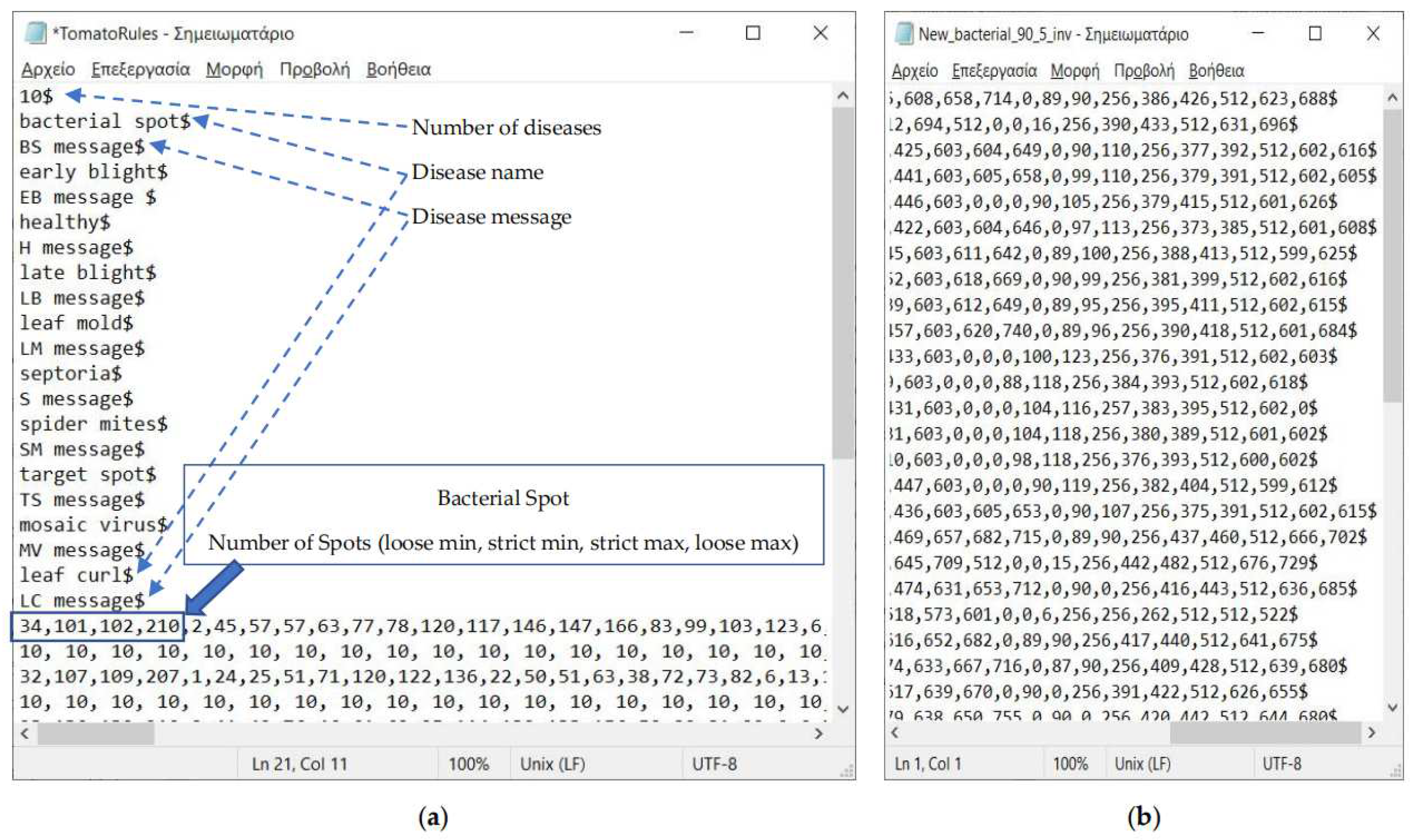
Figure 9 shows the format of the Rules and Range files. In the first line of the Rules file, the number of diseases D is declared. Then, in the following D pairs of rows, the name and the message of each disease are defined. Finally, another set of D pairs follows where the strict/loose ranges of each feature are declared in the first line and the weights in the second. Figure 9a shows an example of range definition for the first feature (Number of Spots) and for the first disease (Bacterial Spot). If different weights have to be given for each feature, the weights in the second row can be altered using a text editor. Part of a Range file is displayed in Figure 9b, where each line contains the feature values from a single training photograph.

3. Experimental Results

In the following experiments with tomato diseases, two splits of the dataset were tested. In the first split (T40), 40 of the 140 photographs of each disease (28.57%) in the dataset were used for training and the rest (100 images, 71.43%) for testing, as described in Section 3.1. The T100 split was tested, as described in Section 3.2. In T100, 100 photographs, i.e., 71.43% of the dataset, were used for training in order to assess the improvement in the classification accuracy with a larger training set. The other 40 photographs (28.57%) were used for testing. In both cases, three feature range configurations were tested: (i) the use of the default strict (50%) and loose (100%) range (Ra), (ii) 50%, 80% and 100% ranges (Rb) and (c) 40%, 50%, 100% and 120% ranges (Rc). A weight equal to five (instead of the default 10) was assigned in the 40%, 80% and 120% ranges. This smaller weight was selected since experiments showed that a higher value increases the bias between hits and misses, i.e., the same samples are still misclassified but with higher confidence. Configuration Rb was selected to investigate the effect of an extra grade that is given if feature values are found in an intermediate range between the strict and the loose one. Configuration Rc was tested to investigate the effect of assigning additional grades for the case where feature values are found in a stricter range than 50% or in a slightly broader range than 100%. A confusion matrix was presented for each one of the combinations that can be defined between Ra, Rb, Rc and T40 and T100. The pear disease dataset was tested, as described in Section 3.3.

Based on the true positive (TP), true negative (TN), false positive (FP) and false negative (FN) samples, the sensitivity, specificity, precision, accuracy and F1 score (classification quality metrics) can be estimated for each disease, as follows:

$$\mathrm{Sensitivity}=\frac{TP}{TP+FN},$$

(4)

$$\mathrm{Specificity}=\frac{TN}{TN+FP},$$

(5)

$$\mathrm{Precision}=\frac{TP}{TP+FP},$$

(6)

$$\mathrm{Accuracy}=\frac{TP+TN}{TP+TN+FN+FP},$$

(7)

$$\mathrm{F}1 \mathrm{score}=\frac{2TP}{2TP+FN+FP},$$

(8)

The experiments showed that most of the early blight test photographs were confused with late blight. However, since both sets described the same disease, the results were unified under the disease name Blight.

3.1. Use of Small Training Set (T40)

Since we desired to demonstrate that the developed classification tools could be trained with a small number of photographs, we initially used 40 out of 140 photographs from each disease for training. The rest of the 100 photographs were used for testing. If the training set was the only set used for testing, the confusion matrix appeared as in

Table 2. Confusion matrix for the training set of T40 and Ra configuration.

Disease	Bacterial Spot	Blight	Healthy	Leaf Mold	Septoria	Spider Mites	Target Spot	Mosaic	Yellow Leaf Curl
Bacterial Spot	36	0	0	0	0	4	0	0	0
Blight	0	80	0	0	0	0	0	0	0
Healthy	2	0	34	4	0	0	0	0	0
Leaf Mold	6	0	2	30	0	2	0	0	0
Septoria	0	0	0	0	40	0	0	0	0
Spider Mites	4	0	2	0	0	34	0	0	0
Target Spot	0	0	0	0	0	0	40	0	0
Mosaic	0	0	0	0	0	0	0	40	0
Yellow Leaf Curled	0	0	0	0	0	0	0	0	40

, and the corresponding classification quality metrics (sensitivity, specificity, precision, accuracy and F1 score) were as listed in

Table 3. Classification quality metrics for the training set of T40 and Ra configuration.

Disease	Sensitivity	Specificity	Precision	Accuracy	F1 Score
Bacterial Spot	90.0%	97.0%	75.0%	96.4%	81.8%
Blight	100.0%	100.0%	100.0%	100.0%	100.0%
Healthy	85.0%	99.0%	89.5%	97.7%	87.2%
Leaf Mold	75.0%	99.0%	88.2%	96.8%	81.1%
Septoria	100.0%	100.0%	100.0%	100.0%	100.0%
Spider Mites	85.0%	98.5%	85.0%	97.3%	85.0%
Target Spot	100.0%	100.0%	100.0%	100.0%	100.0%
Mosaic	100.0%	100.0%	100.0%	100.0%	100.0%
Yellow Leaf Curled	100.0%	100.0%	100.0%	100.0%	100.0%
Average:	92.8%	99.3%	93.1%	98.7%	92.8%

. Similarly, the confusion matrix and the corresponding classification quality metrics for the separate test set consisting of 100 photographs were as listed in

Table 4. Confusion matrix for the test set of T40 and Ra configuration.

Disease	Bacterial Spot	Blight	Healthy	Leaf Mold	Septoria	Spider Mites	Target Spot	Mosaic	Yellow Leaf Curl
Bacterial Spot	74	0	2	10	0	0	0	0	14
Blight	0	196	0	0	4	0	0	0	0
Healthy	36	0	52	10	0	2	0	0	0
Leaf Mold	18	0	2	52	0	16	0	0	12
Septoria	0	28	0	0	72	0	0	0	0
Spider Mites	10	0	14	8	0	68	0	0	0
Target Spot	6	0	0	6	0	4	70	12	2
Mosaic	2	0	0	2	0	0	10	82	4
Yellow Leaf Curled	0	0	6	4	0	0	0	0	90

and

Table 5. Classification quality metrics for the test set of T40 and Ra configuration.

Disease	Sensitivity	Specificity	Precision	Accuracy	F1 Score
Bacterial Spot	74.0%	92.0%	50.7%	90.2%	60.2%
Blight	98.0%	96.9%	87.5%	97.1%	92.5%
Healthy	52.0%	97.3%	68.4%	92.8%	59.1%
Leaf Mold	52.0%	95.6%	56.5%	91.2%	54.2%
Septoria	72.0%	99.6%	94.7%	96.8%	81.8%
Spider Mites	68.0%	97.6%	75.6%	94.6%	71.6%
Target Spot	70.0%	98.9%	87.5%	96.0%	77.8%
Mosaic	82.0%	98.7%	87.2%	97.0%	84.5%
Yellow Leaf Curled	90.0%	96.4%	73.8%	95.8%	81.1%
Average:	73.1%	97.0%	75.8%	94.6%	73.6%

, respectively.

The Rb and Rc configurations were tested for the test set of the 100 photographs, and the resulting confusion matrices and classification quality metrics are listed in

Table 6. Confusion matrix for the test set of T40 and Rb configuration.

Disease	Bacterial Spot	Blight	Healthy	Leaf Mold	Septoria	Spider Mites	Target Spot	Mosaic	Yellow Leaf Curl
Bacterial Spot	62	0	2	10	0	2	0	0	24
Blight	0	196	0	0	4	0	0	0	0
Healthy	42	0	48	10	0	0	0	0	0
Leaf Mold	18	0	2	56	0	14	0	0	12
Septoria	0	42	0	0	58	0	0	0	0
Spider Mites	4	0	12	18	0	64	2	0	0
Target Spot	6	0	2	2	0	8	70	8	4
Mosaic	2	0	0	2	0	0	10	74	12
Yellow Leaf Curled	0	0	8	14	0	2	0	0	76

,

Table 7. Classification quality metrics for the test set of T40 and Rb configuration.

Disease	Sensitivity	Specificity	Precision	Accuracy	F1 Score
Bacterial Spot	62.0%	92.0%	46.3%	89.0%	53.0%
Blight	98.0%	95.3%	82.4%	95.8%	89.5%
Healthy	48.0%	97.1%	64.9%	92.2%	55.2%
Leaf Mold	56.0%	93.8%	50.0%	90.0%	52.8%
Septoria	58.0%	99.6%	93.5%	95.4%	71.6%
Spider Mites	64.0%	97.1%	71.1%	93.8%	67.4%
Target Spot	70.0%	98.7%	85.4%	95.8%	76.9%
Mosaic	74.0%	99.1%	90.2%	96.6%	81.3%
Yellow Leaf Curled	76.0%	94.2%	59.4%	92.4%	66.7%
Average:	67.3%	96.3%	71.5%	93.4%	68.3%

,

Table 8. Confusion matrix for the test set of T40 and Rc configuration.

Disease	Bacterial Spot	Blight	Healthy	Leaf Mold	Septoria	Spider Mites	Target Spot	Mosaic	Yellow Leaf Curl
Bacterial Spot	70	0	2	14	0	0	0	0	14
Blight	0	200	0	0	0	0	0	0	0
Healthy	36	0	46	12	0	4	0	0	2
Leaf Mold	20	2	4	48	0	8	0	0	18
Septoria	0	32	0	0	68	0	0	0	0
Spider Mites	4	0	10	14	0	70	0	0	2
Target Spot	2	0	0	6	0	4	70	10	8
Mosaic	2	0	0	4	0	0	10	72	12
Yellow Leaf Curled	0	0	4	8	0	0	0	0	88

and

Table 9. Classification quality metrics for the test set of T40 and Rc configuration.

Disease	Sensitivity	Specificity	Precision	Accuracy	F1 Score
Bacterial Spot	70.0%	92.9%	52.2%	90.6%	59.8%
Blight	100.0%	96.2%	85.5%	96.9%	92.2%
Healthy	46.0%	97.8%	69.7%	92.6%	55.4%
Leaf Mold	48.0%	93.6%	45.3%	89.0%	46.6%
Septoria	68.0%	100.0%	100.0%	96.8%	81.0%
Spider Mites	70.0%	98.2%	81.4%	95.4%	75.3%
Target Spot	70.0%	98.9%	87.5%	96.0%	77.8%
Mosaic	72.0%	98.9%	87.8%	96.2%	79.1%
Yellow Leaf curled	88.0%	93.8%	61.1%	93.2%	72.1%
Average:	70.2%	96.7%	74.5%	94.1%	71.0%

.

3.2. Use of Large Training Set (T100)

The quality metrics presented in Table 5, Table 7 and Table 9 indicate that, although some particular diseases may be classified with a higher accuracy using Rb or Rc configuration, the average accuracy achieved is better when the default Ra configuration is used. Therefore, the test set of the T100 case was examined only with Ra configuration. The resulting confusion matrix and the classification quality metrics in this case are shown in

Table 10. Confusion matrix for the test set of T100 and Ra configuration.

Disease	Bacterial Spot	Blight	Healthy	Leaf Mold	Septoria	Spider Mites	Target Spot	Mosaic	Yellow Leaf Curl
Bacterial Spot	30	0	0	4	0	0	0	0	6
Blight	0	80	0	0	0	0	0	0	0
Healthy	6	0	30	2	0	0	0	0	2
Leaf Mold	16	0	0	24	0	0	0	0	0
Septoria	0	14	0	0	26	0	0	0	0
Spider Mites	4	0	8	6	0	22	0	0	0
Target Spot	0	0	0	6	0	2	30	2	0
Mosaic	0	0	0	0	0	0	8	32	0
Yellow Leaf Curled	0	0	0	0	0	0	0	0	40

and

Table 11. Classification quality metrics for the test set of T100 and Ra configuration.

Disease	Sensitivity	Specificity	Precision	Accuracy	F1 Score
Bacterial Spot	75.0%	92.8%	53.6%	91.0%	62.5%
Blight	100.0%	95.6%	85.1%	96.5%	92.0%
Healthy	75.0%	97.8%	78.9%	95.5%	76.9%
Leaf Mold	60.0%	95.0%	57.1%	91.5%	58.5%
Septoria	65.0%	100.0%	100.0%	96.5%	78.8%
Spider Mites	55.0%	99.4%	91.7%	95.0%	68.8%
Target Spot	75.0%	97.8%	78.9%	95.5%	76.9%
Mosaic	80.0%	99.4%	94.1%	97.5%	86.5%
Yellow Leaf Curled	100.0%	97.8%	83.3%	98.0%	90.9%
Average:	76.1%	97.3%	80.3%	95.2%	76.9%

, respectively.

3.3. Testing Pear Diseases with Photographs That Are Not Segmented and Normalized

The last experiment conducted was based on the pear disease dataset. As described in Section 2.1, it consisted of 322 images displaying four pear diseases (fire blight: 120 images, fusicladium: 80 images, podosphaera: 82 images and septoria: 40 images). The training set consisted of 20 images from each disease. This means that the fraction of the images that was used for training in each disease was 16.66%, 25%, 24.39% and 50%, respectively. The confusion matrix of this dataset is shown in

Table 12. Confusion matrix for the test set pear diseases and Ra configuration.

Disease	Fire Blight	Fusicladium	Podosphaera	Septoria
Fire blight	30	0	0	4
Fusicladium	0	80	0	0
Podosphaera	6	0	30	2
Septoria	16	0	0	24

. The imbalance in the distribution of the photographs in the training and the test set gave an opportunity for us to study its effect on the achieved accuracy (

Table 13. Classification quality metrics for the test set of pear diseases and Ra configuration.

Disease	Sensitivity	Specificity	Precision	Accuracy	F1 Score
Blight	81.7%	96.7%	90.7%	92.4%	86.0%
Fusicladium	82.5%	95.4%	82.5%	92.7%	82.5%
Podosphaera	100.0%	100.0%	100.0%	100.0%	100.0%
Septoria	90.0%	95.4%	56.3%	95.0%	69.2%
Average:	88.5%	96.9%	82.4%	95.0%	84.4%

).

4. Discussion

Initially, we compared the accuracy achieved in our previous work [27] with the accuracy results presented in Section 3. In [27], five citrus diseases were used as a case study, and they were classified with an accuracy ranging from 73% to 99% per disease and an average accuracy ranging from 84.4% (for photographs captured under direct sunlight) to 90.4% (photographs captured under a canopy). From the detailed experimental results presented in the previous paragraphs, it was deduced that a significant improvement had been achieved since, in Table 5, Table 7, Table 9 and Table 11, the accuracy ranged between 93.4% and 95.2% (average 94.4%). It has to be stressed that, in the present work, the number of supported diseases was doubled (10 tomato diseases), and the aforementioned average accuracy was estimated using a separate test set, while, in [27], the test also included the training set. If we also take into consideration the training set classification results by combining Table 2 and Table 4, the accuracy achieved with Ra configuration is 96.1%.

The significant improvement in the accuracy of the classification results is owed mainly to the different ways that the strict and loose ranges were defined. Defining the strict range of a feature from all the training values, as in [27], ignores the distribution of these values. In this way, a single training feature value that is far from the center of the distribution excessively elongates the strict range. Moreover, the loose range was defined arbitrarily in [27]. This definition lacked a rational justification. The strict and loose ranges were defined in a more sensible way in the updated classification method described here.

The use of multiple ranges also favors a fair disease grading method. Although all the average classification quality metrics (sensitivity, specificity, precision, accuracy, F1 score) were slightly degraded in the Rb and Rc configurations using the T40 training set, specific diseases were classified more accurately. For example, leaf mold was recognized with higher accuracy in Rb and blight and spider mites in Rc. Consequently, these configurations could be useful if a subset of the supported diseases consisting of the diseases that are favored by specific configurations such as Rb and Rc is used. Therefore, the multiple reference ranges supported in the Disease Classifier application can assist the improvement of the classification accuracy in specific sets of diseases.

Increasing the size of the training set from 28.5% to 71.5% of the dataset (and thus decreasing the size of the test set from 71.5% to 28.5%) does not significantly improve the classification quality metrics since the accuracy and the F1 score (which is the harmonic mean of the precision and sensitivity) were increased from 94.6% and 73.6% to 95.2% and 76.9%, respectively, with the Ra configuration. Therefore, it can be argued that, in the proposed classification method, it is sufficient to use a small training set with indicative samples. In contrast with deep learning approaches, the classification accuracy is not affected by the size of the plant part and its orientation. If a system has to be trained with a new set of diseases, a representative, small number of photographs per disease have to be collected, displaying the possible progression stages and coloring variations that can be met when a new photograph is analyzed.

The classification accuracy also depends heavily on the plant species and the plant parts used. In the pear photographs tested in Section 3.3, the number of diseases that had to be discriminated between was smaller than the tomato ones examined in Section 3.1 and Section 3.2. However, three of the four pear diseases are hardly distinguishable. More specifically, podosphaera is easily distinguished due to the white powder look. In contrast, the rest of the diseases show dark spots on the leaf with small differences. Another issue with the pear dataset is the fact that it was imbalanced concerning the number of images that were available for each disease (ranging from 40 septoria to 120 fire blight images). Finally, it was interesting to investigate how the use of photographs that are not segmented or normalized affects the achieved accuracy.

Table 13 shows that the accuracy ranged from 92.4% (fire blight) to 100% for podosphaera. Podosphaera achieved an excellent accuracy due to the fact that it is fully distinguishable from the rest of the diseases. On the other hand, the fact that fire blight achieved the lower accuracy can be explained by the fact that only 16.66% of the dataset was used for training. In septoria, 50% of the dataset was used for training, and the achieved accuracy was 95%. The average accuracy was also 95%, which is slightly better than the one achieved with the tomato diseases, and this is owed to the smaller number of pear diseases that were distinguished. Compared to the citrus diseases examined in [27], a similar study in terms of number of diseases, dataset size and unsegmented photographs, there was a definite improvement of more than 5%. This improvement is owed to the updated classification method and, more specifically, the way that the ranges were defined.

The threshold RGB triplets used per disease in the experiments conducted in Section 3 are shown in

Table 14. Threshold RGB values used per disease.

Disease	R	G	B	Invert
Tomato Bacterial Spot	90	90	90	Yes
Tomato Blight	80	80	80	No
Tomato Healthy	90	90	90	Yes
Tomato Leaf Mold	90	90	90	Yes
Tomato Septoria	100	100	160	No
Tomato Spider Mites	90	90	90	Yes
Tomato Target Spot	100	100	100	Yes
Tomato Mosaic	100	100	100	Yes
Tomato Yellow Leaf Curled	80	80	80	Yes
Pear Fire Blight	40	60	60	No
Pear Fusicladium	20	60	80	No
Pear Podosphaera	40	60	60	Yes
Pear Septoria	40	60	60	No

. Although further customization of the thresholds per photograph can lead to more accurate segmentation, it was preferable to sacrifice some of the segmentation accuracy in order to have a smaller number of predefined thresholds (six triplets covering 13 diseases). The interactive switching between the original and the segmented photograph supported in the Disease Classifier page shown in Figure 7b–e assists the end user with selecting the appropriate thresholds. In a future version of the system, the alternative threshold values will be validated automatically, and the ones that lead to higher segmentation accuracy will be selected based on certain criteria such as the recognized spot area, the distance between the average color level of the spots and the corresponding average color level of the whole leaf, etc. The segmented tomato disease photographs had a black background, thus, the corresponding threshold Tb for each R, G, B color was close to 0: Tb = (5,5,5). The photographs displaying pear diseases were not segmented and normalized, but were captured with the leaves placed on a white sheet or a white bench. The threshold triplet Tb = (120, 160, 220) was used with all pear photographs, leading to a successful background segmentation.

A comparison with some referenced deep learning approaches is shown in

Table 15. Comparison with referenced approaches.

Reference	Accuracy	Notes: Implementation Type, Supported Diseases, Dataset
[4]	92.39% (viral), 95.33% (late blight), 98.56% (bacterial)	CNN, 3 disease states, training:test set ratio = 800:200
[9]	99.55%	ResNet50/101 + SVM classifier, 4 grape diseases (black rot, esca measles, leaf spot, healthy), 423–1383 images/disease
[10]	99.8%	120 classes, pear and apple diseases testing MobileNet and MobileNetV2 on mobile devices, ~10,000 images training:test ratio = 75%:25%
[11]	99.44%, 98.43% and 97.67%	Septoria, Alternaria and Gymnosporangium pear disease with 6 severity levels 4944 pear images. Architecture: VGG16, Inception V3, ResNet50 and ResNet101
[12]	88.8%	CNN, 12 diseases on tomato/potato leafs, training:test ratio = 160:40
[13]	89.2%	MobileNet, 10 tomato leaf diseases 7176 images
[14]	76–100%	CNN, 10 tomato leaf diseases Training:validation:test ratio= 10,000:7000:500
[15]	97.49%	AlexNet, 7 tomato diseases 13,262 segmented images
[16]	Weighted average precision: 96.61% (segmented), 98.61 (unsegmented)	EfficientNet B0, 10 tomato leaf disease 15,000 segmented/unsegmented images
[24]	68.3%	CNN, 5 diseases, training:test ratio= 3000:50
[26]	95.7%	MobileNetV2 + Canny Edge Detection, 26 crop diseases of 14 different species, 87,860 leaf images
This work	94.4%95%	10 tomato diseases, (1400 images) training:test ratio = 400:1000 4 pear diseases (382 images) training:test ratio = 80:302

. Since the compared approaches do not use a common dataset, a fair comparison cannot be performed. However, Table 15 can give a clue about the accuracy achieved in the literature with similar approaches. The applications presented in [10,12,26] concern classification with a higher number of disease cases. The accuracy achieved in [12,13,14,24] was lower than that achieved in our approach. The accuracy achieved in the rest of the approaches was comparable to ours or higher, but most of these approaches support a smaller number of diseases, except for [10,26], where a higher accuracy was achieved for a relatively large number of diseases. The common problem with all the referenced approaches is that their training procedure requires a very large number of photographs. Moreover, they lack extensibility since the end user is not allowed to train the system on new diseases. In our approach, an acceptable accuracy can be achieved by using a relatively small training set consisting of 20–40 photographs per disease. The developed mobile applications can support professional agronomists to customize the supported set of diseases according to the needs of their customers. The resources required by our approach are also negligible since the file with the disease diagnosis rules is just a few kilobytes in size: much smaller than the model files several megabytes in size required by the referenced deep learning approaches.

Concerning the complexity of the proposed approach and its consequent speed, both the training and the test photographs are analyzed almost instantaneously. This is due to the fact that the only time-consuming operations concern the scan of the image: once for segmentation, a second time to merge the spot islands and a third time to create the histograms [27]. Since the images are internally resized to 324 × 182 pixels, the time needed to perform these operations is almost constant. The rest of the operations’ overhead is negligible. Although there is no meaning in giving an exact latency, since it depends on the Android platform used, it can be stated that it is in the order of a few hundreds of milliseconds. Bearing in mind that the user manually selects an image and validates the segmentation quality, most of the time needed to process a photograph is spent in the interaction between a user and the application. Traditional machine learning approaches require several hours to process a large number of training photographs in batch mode. In our approach, training the system with 400 photographs (e.g., 10 diseases with 40 training images per disease) may also require a few hours, but this can be reduced to a few minutes if training is performed in batch mode. Batch mode training will be supported in the next versions of our system when the threshold selection and the background separation will be performed automatically.

5. Conclusions

A pair of mobile disease classification and training tools was described in this paper. The employed classification method is simple and can be implemented efficiently on a smart phone, while, at the same time, it can achieve a remarkable accuracy considering a small training set is used. The architecture of the developed applications and the nature of the employed classification scheme allow the extension of the supported set of diseases by the end user. An average accuracy of about 95% was measured in the various experiments that were conducted.

The most important limitation of the current approach is the separation of complicated backgrounds. Thus, future work will focus on a more sophisticated segmentation approach that separates the background and locates the spots. Another limitation is the dependency on the specific thresholds, although all the experiments were conducted by switching between a very small number of thresholds. The quality of the segmentation is currently assessed interactively by the user, and, therefore, training cannot be performed in batch mode. Addressing this limitation is also part of our future work. Finally, alternative classification methods that can also support an extendible set of diseases will also be investigated.

6. Patents

This work is protected by the patents 1009346/13-8-2018 and 1008484/12-5-2015 (Greek Patent Office).

References

- Sankaran, S.; Mishra, A.; Ehsani, R.; Davis, C. A review of advanced techniques for detecting plant diseases. Comput. Electron. Agric. 2010, 72, 1–13. [Google Scholar] [CrossRef]
- Behmann, J.; Mahlein, A.-K.; Rumpf, T.; Römer, C.; Plümer, L. A review of advanced machine learning methods for the detection of biotic stress in precision crop protection. Precis. Agric. 2014, 16, 239–260. [Google Scholar] [CrossRef]
- Ballesteros, R.; Ortega, J.F.; Hernandez, D.; Moreno, M.A. Applications of georeferenced high-resolution images obtained with unmanned aerial vehicles. Part I: Description of Image Acquisition and Processing. Springer Precis. Agric. 2014, 15, 239–260. [Google Scholar] [CrossRef]
- Xenakis, A.; Papastergiou, G.; Gerogiannis, V.C.; Stamoulis, G. Applying a Convolutional Neural Network in an IoT Robotic System for Plant Disease Diagnosis. In Proceedings of the 11th IEEE International Conference on Information, Intelligence, Systems and Applications (IISA), Piraeus, Greece, 11 December 2020. [Google Scholar] [CrossRef]
- Rodríguez-García, M.; García-Sánchez, F.; Valencia-García, R. Knowledge-Based System for Crop Pests and Diseases Recognition. Electronics 2021, 10, 905. [Google Scholar] [CrossRef]
- Liu, H.; Lee, S.-H.; Chahl, J. A review of recent sensing technologies to detect invertebrates on crops. Precis. Agric. 2016, 18, 635–666. [Google Scholar] [CrossRef]
- Amirruddin, A.D.; Muharam, F.M.; Ismail, M.H.; Tan, N.P.; Ismail, M.F. Hyperspectral spectroscopy and imbalance data approaches for classification of oil palm’s macronutrients observed from frond 9 and 17. Comput. Electron. Agric. 2020, 178, 105768. [Google Scholar] [CrossRef]
- Bhujade, V.G.; Sambhe, V. Role of digital, hyper spectral, and SAR images in detection of plant disease with deep learning network. Multimedia Tools Appl. 2022, 1–26. [Google Scholar] [CrossRef]
- Peng, Y.; Zhao, S.; Liu, J. Fused-Deep-Features Based Grape Leaf Disease Diagnosis. Agronomy 2021, 11, 2234. [Google Scholar] [CrossRef]
- Kodors, S.; Lacis, G.; Zhukov, V.; Bartulsons, T. Pear and apple recognition using deep learning and mobile. Eng. Rural. Dev. 2020, 20, 1795–1800. [Google Scholar]
- Yang, F.; Li, F.; Zhang, K.; Zhang, W.; Li, S. Influencing factors analysis in pear disease recognition using deep learning. Peer-to-Peer Netw. Appl. 2020, 14, 1816–1828. [Google Scholar] [CrossRef]
- Shrestha, G.; Deepsikha; Das, M.; Dey, N. Plant Disease Detection Using CNN. In Proceedings of the IEEE Applied Signal Processing Conference (ASPCON), Kolkata, India, 7 December 2020; pp. 109–113. [Google Scholar] [CrossRef]
- Elhassouny, A.; Smarandache, F. Smart mobile application to recognize tomato leaf diseases using Convolutional Neural Networks. In Proceedings of the 2019 International Conference of Computer Science and Renewable Energies (ICCSRE), Agadir, Morocco, 22–24 July 2019; pp. 10–13. [Google Scholar]
- Agarwal, M.; Singh, A.; Arjaria, S.; Sinha, A.; Gupta, S. ToLeD: Tomato Leaf Disease Detection using Convolution Neural Network. Procedia Comput. Sci. 2020, 167, 293–301. [Google Scholar] [CrossRef]
- Rangarajan, A.K.; Purushothaman, R.; Ramesh, A. Tomato crop disease classification using pre-trained deep learning algorithm. Procedia Comput. Sci. 2018, 133, 1040–1047. [Google Scholar] [CrossRef]
- Bir, P.; Kumar, R.; Singh, G. Transfer Learning based Tomato Leaf Disease Detection for mobile applications. In Proceedings of the IEEE International Conference on Computing, Power and Communication Technologies (GUCON), Greater Noida, India, 2–4 October 2020; pp. 34–39. [Google Scholar] [CrossRef]
- Oteyo, I.N.; Marra, M.; Kimani, S.; De Meuter, W.; Boix, E.G. A Survey on Mobile Applications for Smart Agriculture. SN Comput. Sci. 2021, 2, 293. [Google Scholar] [CrossRef]
- Pérez-Castro, A.; Sánchez-Molina, J.; Castilla, M.; Sánchez-Moreno, J.; Moreno-Úbeda, J.; Magán, J. cFertigUAL: A fertigation management app for greenhouse vegetable crops. Agric. Water Manag. 2017, 183, 186–193. [Google Scholar] [CrossRef]
- Che’Ya, N.N.; Mohidem, N.A.; Roslin, N.A.; Saberioon, M.; Tarmidi, M.Z.; Shah, J.A.; Ilahi, W.F.F.; Man, N. Mobile Computing for Pest and Disease Management Using Spectral Signature Analysis: A Review. Agronomy 2022, 12, 967. [Google Scholar] [CrossRef]
- Johannes, A.; Picon, A.; Alvarez-Gila, A.; Echazarra, J.; Rodriguez-Vaamonde, S.; Navajas, A.D.; Ortiz-Barredo, A. Automatic plant disease diagnosis using mobile capture devices, applied on a wheat use case. Comput. Electron. Agric. 2017, 138, 200–209. [Google Scholar] [CrossRef]
- Adam, A.; Kho, P.E.; Sahari, N.; Tida, A.; Chen, Y.S.; Tawie, K.M.; Kamarudin, S.; Mohamad, H. Dr.LADA: Diagnosing Black Pepper Pests and Diseases with Decision Tree. Int. J. Adv. Sci. Eng. Inf. Technol. 2018, 8, 1584–1590. [Google Scholar] [CrossRef] [Green Version]
- Toseef, M.; Khan, M.J. An intelligent mobile application for diagnosis of crop diseases in Pakistan using fuzzy inference system. Comput. Electron. Agric. 2018, 153, 1–11. [Google Scholar] [CrossRef]
- Moawad, N.; Elsayed, A. Smartphone Application for Diagnosing Maize Diseases in Egypt. In Proceedings of the 14th IEEE International Conference on Innovations in Information Technology (IIT), Al Ain, United Arab Emirates, 25 December 2020; pp. 24–28. [Google Scholar] [CrossRef]
- Moloo, R.K.; Caleechurn, K. An App for Fungal Disease Detection on Plants. In Proceedings of the 2022 International Conference for Advancement in Technology (ICONAT), Goa, India, 21–22 January 2022; pp. 1–5. [Google Scholar] [CrossRef]
- Loyani, L.; Machuve, D. A Deep Learning-based Mobile Application for Segmenting Tuta Absoluta’s Damage on Tomato Plants. Eng. Technol. Appl. Sci. Res. 2021, 11, 7730–7737. [Google Scholar] [CrossRef]
- Shrimali, S. PlantifyAI: A Novel Convolutional Neural Network Based Mobile Application for Efficient Crop Disease Detection and Treatment. Procedia Comput. Sci. 2021, 191, 469–474. [Google Scholar] [CrossRef]
- Petrellis, N. Plant Disease Diagnosis for Smart Phone Applications with Extensible Set of Diseases. Appl. Sci. 2019, 9, 1952. [Google Scholar] [CrossRef] [Green Version]
- Petrellis, N. A Review of Image Processing Techniques Common in Human and Plant Disease Diagnosis. Symmetry 2018, 10, 270. [Google Scholar] [CrossRef] [Green Version]
- PlantVillage Dataset. Available online: https://www.kaggle.com/datasets/abdallahalidev/plantvillage-dataset (accessed on 1 May 2022).
- Parraga-Alava, J.; Cusme, K.; Loor, A.; Santander, E. RoCoLe: A robusta coffee leaf images dataset for evaluation of machine learning based methods in plant diseases recognition. Data Brief 2019, 25, 104414. [Google Scholar] [CrossRef] [PubMed]
- Parraga-Alava, J.; Alcivar-Cevallos, R.; Carrillo, J.M.; Castro, M.; Avellán, S.; Loor, A.; Mendoza, F. LeLePhid: An Image Dataset for Aphid Detection and Infestation Severity on Lemon Leaves. Data 2021, 6, 51. [Google Scholar] [CrossRef]
- Petrellis, N. Plant Disease Diagnosis with Color Normalization. In Proceedings of the 8th International Conference on Modern Circuits and Systems Technologies, MOCAST, Thessaloniki, Greece, 13–15 May 2019. [Google Scholar]
Figure 1.
Sample photographs from each one of the supported tomato leaf diseases: (a) bacterial spot; (b) early blight; (c) late blight; (d) healthy; (e) leaf mold; (f) septoria leaf spot; (g) spider mites; (h) target spot; (i) mosaic virus; (j) yellow leaf curl virus.
Figure 2.
Sample photographs from each one of the supported pear leaf diseases: (a) fire blight; (b) fusicladium; (c) podosphaera; (d) septoria.
Figure 3.
The steps followed in the image processing, classification and training procedure.
Figure 4.
Image segmentation for yellow leaf curl disease: (a) original image; (b) segmented image.
Figure 5.
Example RGB histograms.
Figure 6.
Feature range definition.
Figure 7.
Disease Classifier pages. (a) Entry page; (b) range definition; (c) image selection; (d) image segmentation; (e) spot histograms; (f) classification results.
Figure 8.
Disease Classifier and Disease Classification Trainer pages involved in the training process.
Figure 9.
File formats. Rules file format (a); range file format (b).