
Detection of Power Poles in Orchards Based on Improved Yolov5s Model
by
 ,
,
Yali Zhang
1,2,
Xiaoyang Lu
1,2,
Wanjian Li
1,2,
Kangting Yan
2,3,
Zhenjie Mo
1,2,
Yubin Lan
2,3 and
Linlin Wang
4,* 1
College of Engineering, South China Agricultural University, Guangzhou 510642, China
2
National Center for International Collaboration Research on Precision Agricultural Aviation Pesticides Spraying Technology, Guangzhou 510642, China
3
College of Electronic Engineering, South China Agricultural University, Guangzhou 510642, China
4
School of Artificial Intelligence, Shenzhen Polytechnic University, Shenzhen 518055, China
*
Author to whom correspondence should be addressed.
Agronomy 2023, 13(7), 1705; https://0-doi-org.brum.beds.ac.uk/10.3390/agronomy13071705
Submission received: 25 May 2023
/
Revised: 21 June 2023
/
Accepted: 24 June 2023
/
Published: 26 June 2023
(This article belongs to the Special Issue New Trends in Agricultural UAV Application)
Abstract
:During the operation of agricultural unmanned aerial vehicles (UAVs) in orchards, the presence of power poles and wires pose a serious threat to flight safety, and can even lead to crashes. Due to the difficulty of directly detecting wires, this research aimed to quickly and accurately detect wire poles, and proposed an improved Yolov5s deep learning object detection algorithm named Yolov5s-Pole. The algorithm enhances the model’s generalization ability and robustness by applying Mixup data augmentation technique, replaces the C3 module with the GhostBottleneck module to reduce the model’s parameters and computational complexity, and incorporates the Shuffle Attention (SA) module to improve its focus on small targets. The results show that when the improved Yolov5s-Pole model was used for detecting poles in orchards, its accuracy, recall, and mAP@50 were 0.803, 0.831, and 0.838 respectively, which increased by 0.5%, 10%, and 9.2% compared to the original Yolov5s model. Additionally, the weights, parameters, and GFLOPs of the Yolov5s-Pole model were 7.86 MB, 3,974,310, and 9, respectively. Compared to the original Yolov5s model, these represent compression rates of 42.2%, 43.4%, and 43.3%, respectively. The detection time for a single image using this model was 4.2 ms, and good robustness under different lighting conditions (dark, normal, and bright) was demonstrated. The model is suitable for deployment on agricultural UAVs’ onboard equipment, and is of great practical significance for ensuring the efficiency and flight safety of agricultural UAVs.
1. Introduction
The planting of fruit trees is an important part of China’s agricultural production structure, and the application of agricultural UAVs in orchards has been effective [1,2,3]. However, the operating environment of orchards is complex, and collisions with power lines are the main cause of agricultural UAV crashes [4,5]. Due to the complexity and variability of the orchard environment and the limitations of different sensor applicability ranges, there is a problem that obstacle avoidance sensors cannot effectively detect power line obstacles directly [6]. For only detecting the power lines themselves, the technical difficulty is high, and it is difficult to achieve maturity in the short term. Therefore, we consider an indirect recognition method, which recognizes substitutes for power lines such as the power pole or tower [7], and establish a feature database of relevant obstacle substitutes to propose a detection model that can be lightweight and deployed on agricultural UAVs. It can not only effectively improve the detection success rate of power line obstacles, but also improves the safety and efficiency of agricultural UAV orchard operations [8,9], promoting the mechanization process of orchards, and providing support for orchard plant protection [10,11], fruit tree pollination [12,13], information collection [14,15], monitoring and warning [16,17], which have practical production significance.
According to the research trends of industry, academia, and research institutions in recent years, it can be found that the current mainstream trend of obstacle avoidance research uses multi-sensor fusion of vision and non-vision [18,19,20] to identify field obstacles and improve plant protection operations. Qiu et al. [21] installed a machine vision system consisting of an RGB camera and a desktop computer on a paddy transplanter using an improved Yolov3 and deep SORT combined method to detect and track typical moving obstacles in the paddy field, such as people and water buffalo, and calculated the center point position of them. The results showed that the improved Yolov3 model had a processing speed that was 27.3% faster than the original Yolov3 module. In actual rice field tests, the average processing speed was 5–7 FPS, but this processing speed is difficult to meet the needs of detecting and tracking targets in actual UAV operations; furthermore, this machine vision system is too heavy to mount. Chen et al. [22] proposed an improved Yolov3-tiny target detection model, which uses a panoramic camera mounted on the top of the agricultural machinery to obtain 360° image information, and quickly detects field pedestrians and other agricultural machinery. The average accuracy and recall rates were 95.5% and 93.7%, respectively, which were 5.6% and 5.2% higher than the original network model, respectively. The average time for detecting a single panoramic image was 6.3 ms, and the average frame rate for video stream detection was 84.2 FPS. However, the model’s memory requirement of 64 MB renders it unsuitable for embedded devices and deployment. Chen et al. [23] proposed an innovative solution based on Yolov3 for the detection and pole counting of UAV patrol video distribution poles. The detection accuracy of this method was higher than 0.9. However, the high shooting angle of this method is not applicable to the working height of agricultural UAVs, and the effect of lighting on identification was not mentioned in the study.
Due to the limited arithmetic power of the embedded devices carried by agricultural UAVs [24,25], lightweight models are commonly selected for target recognition. Liu et al. [26] proposed an improved SSD (Single Shot MultiBox Detector) insulator and spacer detection algorithm that uses a lightweight network, MnasNet, as a feature extraction network to generate feature maps. Then, two multi-scale feature fusion methods were used to fuse multiple feature maps. The detection accuracy was up to 93.8%. The detection time for a single image on NVIDIA Jetson TX2 was 154 ms, and the capture rate on TX2 was 8.27 fps. Yu et al. [27] proposed a new lightweight neural network called TasselLFANet, which was specifically designed for the accurate and efficient detection and computation of maize male ears in high spatio-temporal image sequences. The method enhances the feature learning capability of TasselLFANet by employing a cross-stage fusion strategy that balances the variability of different layers. In addition, TasselLFANet utilizes multiple receptive fields to capture different feature representations, and incorporates an innovative visual channel attention module that allows for more flexible and accurate feature detection and capture. The network achieves impressive evaluation metrics, with F1 and mAP@50 scores of 94.4% and 96.8%, respectively, while only consisting of 6.0 M parameters.
Therefore, this study optimizes the Yolov5s model with the Shuffle Attention module to focus on important feature learning and reduce the interference of non-critical information. At the same time, to meet the real-time detection needs of embedded modules in agricultural UAVs, the model is made lightweight by replacing the C3 module with the GhostBottleneck module. To solve the problem of a small number of datasets, the Mixup data augmentation technique is used to propose a lightweight detection model Yolov5s-Pole based on Yolov5s, which is specifically used to detect orchard power poles, in order to improve the operation safety of agricultural UAVs and promote the mechanization process of orchards.
2. Materials and Methods
2.1. Power Pole Data Collection
There is no publicly available dataset that contains exactly the same content. Therefore, it was necessary to establish a relevant dataset applicable to this study. The dataset we used was collected from the Cuitian Orange Orchard in Sihui City, Guangdong Province. The planting area of Shatang oranges in the orchard in 2021 exceeded 1000 mu, and various common power poles and other pole-shaped obstacles were distributed throughout the orchard. The data were collected twice, from the end of July to early August 2021, by the DJI aerial survey UAV Phantom 4 RTK. In order to obtain more power pole data in a variety of scenes, the flight speed was set to 2 m/s, and the flight altitude was set to 1–5 m above the citrus canopy, with an absolute altitude of 3–8 m.
Due to the possibility of motion blur caused by UAV steering, the lack of specific operational obstacles, or a high similarity between adjacent frames in the exported images, it was necessary to manually filter the image set to form a preliminary dataset. After screening, the self-built dataset had a total of 305 images as original images, and the training set, validation set, and test set were divided into a ratio of 8:1:1. The power poles in the original images were manually labeled with LabelImg annotation tool, and the label for power poles was set as pole. The operating interface is shown in Figure 1, and the computer configuration used is shown in Table 1.
2.2. Introduction of Yolov5s Model
Yolov5 is an object detection model, and implemented in PyTorch. The model uses a new network structure called CSP (Cross-Stage Partial Network), which effectively reduces computation while retaining the original network characteristics. It also has innovative features such as adaptive anchor box calculation and adaptive image scaling. Yolov5 has multiple versions, including Yolov5s, Yolov5m, Yolov5l, and Yolov5x. This study used the Yolov5s model, including the input, backbone, neck, and prediction parts. The Yolov5s model uses rich data augmentation techniques during training, such as random size, proportional image clipping, random flip, random rotation, and random adjustments to brightness, contrast, and color balance. The improved Yolov5s-Pole model structure is shown in Figure 2.
2.3. Model Improvement
2.3.1. Mixup Data Enhancement
Mixup is a data augmentation technique that is based on sample interpolation [28]. It is used to increase the diversity of neural network training data, thereby improving the model’s generalization ability and robustness. Mixup combines two samples and their label data in proportion to create new sample and label data.
In Equations (1) and (2), and are the samples of the two inputs; with are the labels of the two inputs; and and are the new samples and the new labels of the output, respectively. , .
It can be seen from Figure 3 that when α = β = 1, the Beta distribution is equivalent to a uniform distribution with y = 1; when α = β < 1, the probabilities at both ends of the Beta distribution are higher than those in the middle; when α = β → 0, the Beta distribution is equivalent to a binomial distribution with x = 0, 1, indicating no data enhancement; when α = β > 1, the probabilities at both ends of the Beta distribution are lower than those in the middle, similar to a normal distribution; when α = β → ∞, the probabilities of the Beta distribution are always 0.5, equivalent to taking half of each of two samples. Therefore, using the Beta distribution for data augmentation is very flexible, and various probability distributions within the [0, 1] range can be obtained by adjusting the values of α and β, making it very convenient to use.
2.3.2. Replace the GhostBottleneck Module
GhostBottleneck is a network structure design method for deep neural networks that is aimed at reducing the number of model parameters and computational complexity while improving model performance [29]. The Ghost module divides the original convolution operation into two stages. In the first stage, half of the original convolution is used to generate a small number of feature maps. In the second stage, a 3 × 3 small convolution is used to convolve the feature maps obtained in the first stage, layer by layer, to obtain more feature maps. Finally, these feature maps are combined together. The number of feature maps obtained after the two-stage calculation in the Ghost module is consistent with the number of feature maps obtained by normal convolution operation.
As shown in Figure 4, GhostBottleneck consists of two Ghost modules. The first Ghost module increases the input feature map channel number, and the second Ghost module reduces the output feature map channel number. The two Ghost modules are connected by a diameter structure, and the first Ghost module uses the ReLU activation function, while the subsequent layers use batch normalization. In this way, GhostBottleneck can reduce model parameters and computational complexity while optimizing feature maps and improving model detection efficiency.
2.3.3. Adding SA Module
The attention mechanism is an important component of deep neural networks; it can accurately focus on input-related information to improve network performance. There are mainly two types of attention mechanisms in the computer vision field, the spatial attention mechanism and the channel attention mechanism, which capture the relationships between pixels and channel dependencies, respectively. Combining these two attention mechanisms may achieve better performance, but this increases computational costs. The SA module can efficiently combine these two attention mechanisms [30].
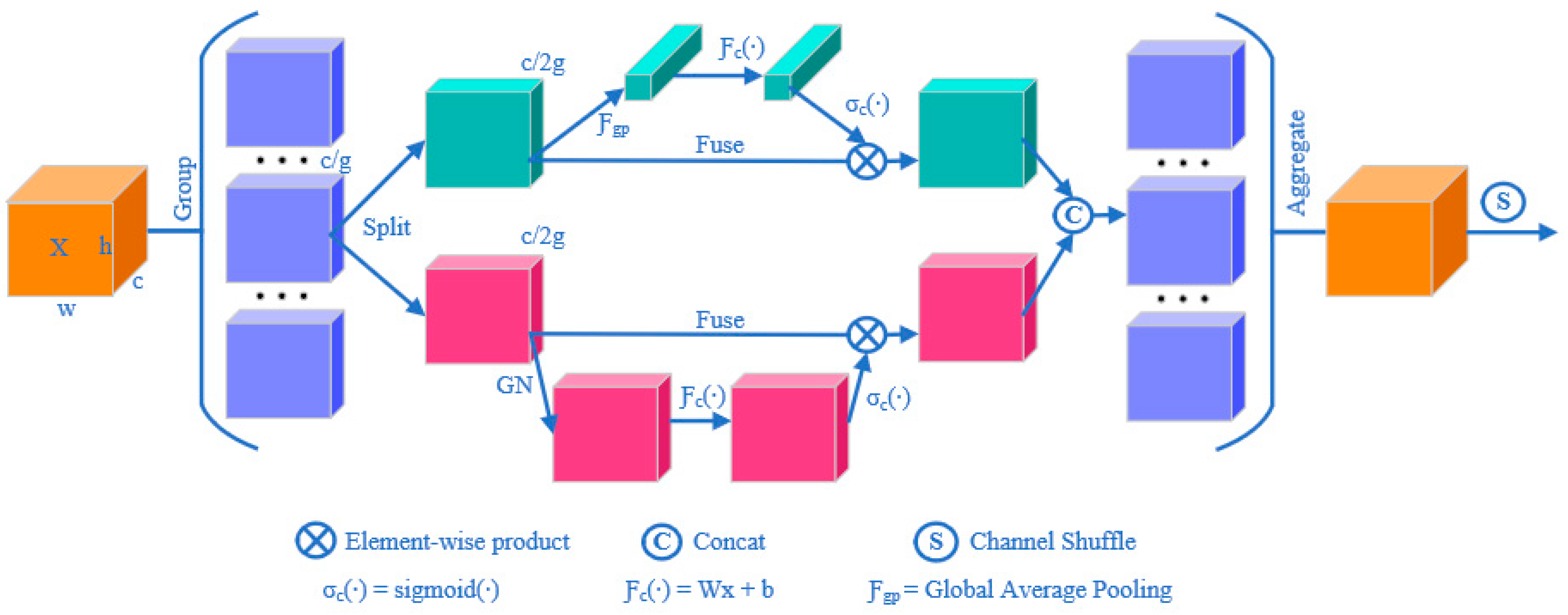
As shown in Figure 5, the input feature map is grouped and used as an SA unit. Each SA unit is divided into two parts, with one part using channel attention, as shown in the red part of the figure; the specific implementation is similar to the SE attention mechanism, and the other part uses spatial attention, as shown in the green part of the figure; GN means group normalization. The two internal parts of the SA unit are stacked by the channel number to achieve information fusion. Finally, a random mixing operation is performed on all SA units to obtain the final output feature map.
2.4. Model Evaluation Indicators
Commonly used in target recognition tasks, the evaluation indicators precision, recall, and mAP@50 are derived based on comparisons between the model prediction results and true labels.
- Precision refers to the proportion of predicted power poles that are truly power poles. For the proportion of correctly predicted samples to the number of samples predicted as power poles, the calculation formula is as follows:
In Equation (3), TP represents the number of samples that are truly power poles, and FP represents the number of samples that are incorrectly predicted as power poles.
- 2.
- Recall refers to the proportion of truly power pole samples that are correctly predicted to be power poles. The calculation formula is as follows:
In Equation (4), TP represents the number of truly power pole samples, and FN represents the number of samples predicted as background, but are actually power poles.
- 3.
- mAP@50 is a composite indicator. mAP@50 is obtained by calculating the area under the precision and recall curves with the following formula. Specifically, mAP@50 is the average value of AP that calculated for all categories when the IoU threshold is 0.5.
In the target recognition task, precision and recall are two important evaluation indicators that can be used to measure the performance of the model in terms of prediction accuracy and coverage. The mAP@50 is a comprehensive evaluation of precision and recall, which can evaluate the performance of the model more comprehensively.
3. Results
The following model training hyperparameters are uniformly used in the following experiments, as shown in Table 2.
3.1. Yolov5s Experiment
In the initial experiments, different input image sizes were chosen for training, 416 × 416, 512 × 512, and 640 × 640, and their effects on the experimental results were compared. The results are shown in Table 3, and it can be seen from the data that the evaluation metrics of the model all improve as the image size increases. Particularly, the best results were achieved with an image size of 640 × 640, although this also resulted in increased recall and inference time. This can be attributed to the fact that a larger image size provides more information, making the model easier to find the target object. Both precision and mAP@50 showed a small improvement when the size was increased from 416 to 512, but the recall remained the same. This can be explained by the higher resolution offering more information, thereby aiding the model in accurately locating the target object. However, when the size was further increased to 640, the model’s recall and mAP@50 also improved, but its precision slightly decreased. This could be due to the fact that the larger image size increases the computational and time costs, making the model less efficient in processing large-size images.
Brightness is one of the important factors affecting image recognition [31], because changes in brightness affect the contrast and color distribution of the image, which affects the recognition ability of the model. To better understand the effect of brightness on image recognition, the OpenCV library was used to convert images to grayscale images and calculate the average brightness value of grayscale images. For the average brightness value, the range of the dataset was 52–198, according to the size of the average brightness value of the image and considering the distribution of the number of datasets after classification. It was divided into three parts, which are dark (52–98), medium (98–112), and bright (112–198). The light in the dark dataset was weak, and the color of the power poles in the image was more similar to the background, which made recognition difficult, and the power poles in individual images needed to be seen by magnifying the image. In the medium dataset, the light was normal, and the poles were better distinguished from the background, which was easier to recognize. For the bright dataset with sufficient light, power poles could be unclear in the sky background, which may lead to incomplete recognition, as shown in Figure 6. Experiments were conducted on the poles under different luminance conditions, and the results are shown in Table 4. It can be seen that the recognition accuracy and the average accuracy of the model improved with an increase in the brightness, and the inference time also increased. In particular, the model had the best recognition effect under bright light conditions, while recall and precision also improved. This may be due to the fact that the contrast and color distribution of the image were more obvious under bright light conditions, helping the model to more easily and accurately recognize objects in the image. On the contrary, in the dark light condition, the model had the worst recognition effect, with low recall and precision. In such conditions, the blurred contrast and color distribution made it challenging for the model to accurately detect objects.
There were some problems in the recognition of power poles using the Yolov5s model, such as false recognition, an inability to recognize occlusion, inaccurate recognition of multiple targets, and incomplete recognition, as shown in Figure 7. All of these problems affected the recognition accuracy and robustness of the model, and subsequent improvement experiments will address and optimize these existing problems.
3.2. Experiment with the Improved Yolov5s
3.2.1. Ablation Experiments
In order to verify the optimization effect of each improved module on the Yolov5s model, ablation experiments were conducted on the modules, as shown in Table 5. The constructed pole datasets were trained and tested separately, and the experimental results are shown in Table 6.
After a comparative analysis, it was found that the group with the lowest precision score was group A (0.798), and the highest was group C (0.864). Except for group A, the precision scores of the other groups were all above 0.8. The group with the lowest recall score was group A (0.731), and the highest was group F (0.831). Except for groups E and F, the recall scores of the other groups were below 0.8. The group with the lowest mAP@50 score was group A (0.746) and the highest was group F (0.838), while groups B and E also performed well. Overall, all three evaluation metrics for Group A were below 0.8, which also were the lowest. The best results were found in group F, where all three evaluation metrics were above 0.8, with recall and mAP@50 being the highest values.
All three improved modules improved the evaluation metrics for the model. Mixup increased the recall and mAP@50 metrics by 0.027 and 0.09, respectively, while reducing the inference time by 0.1 ms. GhostBottleneck improved the precision metric of the model by 0.066, increased the number of layers by 57, but reduced the weight by 5.74 MB, and decreased the number of parameters by 3,048,208, reduced GFLOPs by 6.9, and also reduced the inference time by 2.3 ms. SA has improved the recall and mAP@50 metrics of the model combined with Mixup and GhostBottleneck by 0.031 and 0.026, respectively, but increased the inference time by 0.1 ms. Compared to the Yolov5s model, the improved Yolov5s-Pole model improved the precision, recall, and mAP@50 metrics by 0.005, 0.1, and 0.092, respectively. It is worth noting that there is a certain balance between the precision and recall metrics; improving one metric may reduce the other, so the balance of the two metrics should be considered comprehensively. Overall, the improved model showed significant progress in all three metrics.
3.2.2. Different Brightness Comparison
Ablation experiments were carried out to investigate the effect of the improved module with different brightness datasets. Test datasets with different brightness were used in the experiments, and the performance with or without the improvement module was compared; the results are shown in Table 7.
For the three types of datasets, the brighter the dataset was, the higher the three evaluation metrics were, and the higher the upper and lower bounds were. The evaluation metrics of the model were improved by the three improvement modules. The SA module alone did not improve the evaluation metrics as much as the other two modules, but the effect was significant when combined with the other two modules; comparing Group E and Group F on the bright dataset, the improvement in precision, recall, and mAP@50 metrics were 0.056, 0.106, and 0.075, respectively, but the effect on the ark dataset was less effective. This may be due to the fact that the model generated more interest in regions with high brightness, and thus gained more attention. Comparing the different datasets, group F was better than group A in all cases.
3.2.3. Comparison of Yolov5s-Pole and Yolov5s Effects
In response to the problems of false recognition, an inability to recognize occlusion, inaccurate recognition of multiple targets, and incomplete recognition when Yolov5s model recognizes power poles, Yolov5s-Pole solved and optimized the existing problems and obtained better results and higher confidence, as shown in Figure 8.
4. Discussion
4.1. Comparison of Different Models
For the Yolov5-Pole model proposed in this study with different versions of the Yolov5 and Yolov7-tiny models [32], a comprehensive performance comparison was conducted, and the results are shown in Table 8. Collectively, the different versions of the Yolo model differ in terms of their accuracy, model size, and inference speed.
Among them, the Yolov5-Pole model performed best in the recall and mAP@50 metrics, while the Yolov5l model performed best in the precision metric. The Yolov5-Pole model had the smallest weight, parameters, and GFLOPs, which were 42.2%, 42.4%, and 43.3% less than the Yolov5s model, respectively. It was the lightest model among all of the models. In terms of layers, the Yolov5-Pole model had 275 layers, which was 61 more than the smallest Yolov5s model; however, thanks to the smaller number of parameters, the actual running time was faster than the Yolov5s model. The fastest inference time was for the Yolov7-tiny model, but the Yolov5-Pole model did not perform poorly either, being 35.3% faster than the Yolov5s model.
The network structures of the Yolov5m and Yolov5l models are relatively large, but the results did not significantly improve. This may be attributed to the fact that the larger the deep learning network is, the number of parameters and computation time of the model increases, leading to a more complex model and increased time and resource consumption for training and inference. This may lead to problems such as overfitting, gradient disappearance, and gradient explosion, resulting in a decrease in the performance of the model.
Moreover, the Yolov5-Pole model achieved the best results with the smallest network structure. It is possible that for some simple tasks and small datasets, smaller deep learning networks may perform better. Smaller networks are more likely to learn patterns and features in the data, while being less prone to overfitting. In this case, choosing a smaller network can improve the performance and effectiveness of the model. Therefore, when choosing a deep learning network size, it is necessary to select the most suitable network size according to specific application scenarios and datasets, in order to achieve the best performance and effect.
4.2. The Effect of Brightness
When performing a model target recognition task, changes in brightness have a significant impact on the recognition results. Brightness variations affect the appearance of the target in the image, thereby diminishing target recognizability. In low-light conditions, details and edges of the target may be blurred or lost, leading to situations such as missed recognition or false recognition. In the test dataset, these situations mainly occurred in the dark dataset. Therefore, to improve the recognition of the model in low-light conditions, HDR (High Dynamic Range) techniques can be considered to capture images to obtain richer lighting information. In addition, models with robustness, such as those with better robustness to noise and illumination changes, can also be considered for model training to improve the recognition ability of the model. When data acquisition is performed, it should be selected under well-lit conditions as much as possible to improve the quality of the data and, consequently, the accuracy of target recognition [33]. These measures can be combined to improve the recognition performance of the model, and thus better cope with the target recognition tasks under different lighting conditions.
4.3. Adding Identification Classes
In orchard obstacle recognition applications, UAVs can add the recognition of classes such as people and power lines, in addition to recognizing common obstacles such as power poles [34]. These obstacles often appear in UAV operations, so the ability of UAVs to identify the locations of people and power lines can effectively improve the safety and efficiency of operations. For example, when a UAV sprays pesticides, if a person appears in the spraying area, the UAV can automatically stop spraying by recognizing the location of the person, thus avoiding the harm of exposing human beings to toxic pesticides. In addition, UAVs can also help farmers better plan the paths of UAV operations by identifying the locations of power lines. This can avoid collisions between UAVs and power lines and improve operational efficiency and safety. Therefore, for UAV farming operations, it is important to accurately identify and locate these obstacles, which helps to guarantee safer and more efficient agricultural production.
5. Conclusions
The relevant safety distance is determined according to the obstacle category to guarantee the safety of personal and public property. This study used a lightweight deep learning model to enable the rapid deployment of performance-limited embedded devices on agricultural UAVs. It was able to complete obstacle recognition and detection of specific operations in planting orchards. After improvements, the model’s performance was re-evaluated, and the detection results were analyzed. When the improved Yolov5s-Pole model was applied to orchard poles recognition detection, it performed as follows: precision of 80.3%, recall of 83.1%, and mAP@50 of 83.8%. Compared with the previous model, the improvements in these evaluation metrics were by 0.5%, 10%, and 9.2%, respectively. The model weights were compressed from the original version of 13.6 M to 7.86 M, and the model was reduced by 42.2%. The parameters and GFLOPs were compressed by 43.4% and 43.3% to 3,974,310 and 9, respectively. The single-image detection time was 4.2 ms, which indicates that the Yolov5s-Pole model can fully meet the real-time detection needs of orchard obstacles in the working state of the visual module. It was also shown that the Yolov5s-Pole model achieved a significant degree of compression on the basis of basic retention of the original model’s performance, which is beneficial to lightweight deployment on the airborne visual module. In future developments, the recognition of more types of obstacles on agricultural UAVs can be added. As the technology continues to advance and the arithmetic power increases, more target recognition models and algorithms can be explored and applied to expand the recognition capability of UAVs.
Author Contributions
Conceptualization, methodology, software, Y.Z. and X.L.; validation, Y.Z., X.L. and Z.M.; formal analysis, X.L. and Z.M.; investigation, X.L., L.W. and W.L.; resources, L.W. and W.L.; data curation, X.L., K.Y. and Z.M.; writing—original draft preparation, X.L. and L.W.; writing—review and editing, L.W., K.Y. and W.L.; visualization, Y.Z. and X.L.; supervision, X.L.; project administration, Y.Z.; funding acquisition, Y.Z. and Y.L. All authors have read and agreed to the published version of the manuscript.
Funding
This research was funded by the Laboratory of Lingnan Modern Agriculture Project, grant number NT2021009, the Key Field Research and Development Plan of Guangdong Province, China, grant number 2019B020221001, and the 111 Project, grant number D18019.
Data Availability Statement
The data presented in this study are available on request from the corresponding author. The data are not publicly available due to the multiple interests involved in the data.
Acknowledgments
Special thanks to Huanzhou Cui for writing assistance.
Conflicts of Interest
The authors declare no conflict of interest.
References
- Lan, Y.; Chen, S. Current Status and Trends of Plant Protection UAV and Its Spraying Technology in China. Int. J. Precis. Agric. Aviat. 2018, 1, 1–9. [Google Scholar] [CrossRef]
- Yang, S.; Yang, X.; Mo, J. The Application of Unmanned Aircraft Systems to Plant Protection in China. Precis. Agric. 2018, 19, 278–292. [Google Scholar] [CrossRef]
- Huang, Y.; Thomson, S.J.; Hoffmann, W.C.; Lan, Y.; Fritz, B.K. Development and Prospect of Unmanned Aerial Vehicle Technologies for Agricultural Production Management. Int. J. Agric. Biol. Eng. 2013, 6, 1–10. [Google Scholar] [CrossRef]
- Xiongkui, H.; Bonds, J.; Herbst, A.; Langenakens, J. Recent Development of Unmanned Aerial Vehicle for Plant Protection in East Asia. Int. J. Agric. Biol. Eng. 2017, 10, 18–30. [Google Scholar] [CrossRef]
- Uche, U.E.; Audu, S.T. UAV for Agrochemical Application: A Review. Niger. J. Technol. 2021, 40, 795–809. [Google Scholar] [CrossRef]
- Wang, L.; Lan, Y.; Zhang, Y.; Zhang, H.; Tahir, M.N.; Ou, S.; Liu, X.; Chen, P. Applications and Prospects of Agricultural Unmanned Aerial Vehicle Obstacle Avoidance Technology in China. Sensors 2019, 19, 642. [Google Scholar] [CrossRef] [Green Version]
- Qian, S.; Dai, S. Identification of High-Speed Railway Trackside Equipments Based on YOLOv4. In Proceedings of the 2022 China Automation Congress (CAC), Xiamen, China, 25–27 November 2022; pp. 3635–3640. [Google Scholar]
- Clothier, R.; Walker, R. Determination and Evaluation of UAV Safety Objectives. In Proceedings of the 21st International Conference on Unmanned Air Vehicle Systems, Dubrovnik, Croatia, 21–24 June 2022; Hugo, S., Ed.; University of Bristol: Bristol, UK, 2006; pp. 18.1–18.16. ISBN 978-0-9552644-0-5. [Google Scholar]
- Balestrieri, E.; Daponte, P.; De Vito, L.; Picariello, F.; Tudosa, I. Sensors and Measurements for UAV Safety: An Overview. Sensors 2021, 21, 8253. [Google Scholar] [CrossRef]
- Cao, G.; Li, Y.; Nan, F.; Liu, D.; Chen, C.; Zhang, J. Development and Analysis of Plant Protection UAV Flight Control System and Route Planning Research. Trans. Chin. Soc. Agric. Mach. 2020, 51, 1–16. [Google Scholar]
- ShengDe, C.; YuBin, L.; ZhiYan, Z.; JiYu, L.; Fan, O.; XiaoJie, X.; WeiXiang, Y. Test and evaluation for flight quality of aerial spraying of plant protection UAV. J. South China Agric. Univ. 2019, 40, 89–96. [Google Scholar]
- Chen, Y.; Pi, D.; Xu, Y. Neighborhood Global Learning Based Flower Pollination Algorithm and Its Application to Unmanned Aerial Vehicle Path Planning. Expert Syst. Appl. 2021, 170, 114505. [Google Scholar] [CrossRef]
- Broussard, M.A.; Coates, M.; Martinsen, P. Artificial Pollination Technologies: A Review. Agronomy 2023, 13, 1351. [Google Scholar] [CrossRef]
- Wang, X.; Sun, H.; Long, Y.; Zheng, L.; Liu, H.; Li, M. Development of Visualization System for Agricultural UAV Crop Growth Information Collection. IFAC-PapersOnLine 2018, 51, 631–636. [Google Scholar] [CrossRef]
- Tsouros, D.C.; Bibi, S.; Sarigiannidis, P.G. A Review on UAV-Based Applications for Precision Agriculture. Information 2019, 10, 349. [Google Scholar] [CrossRef] [Green Version]
- Xie, C.; Yang, C. A Review on Plant High-Throughput Phenotyping Traits Using UAV-Based Sensors. Comput. Electron. Agric. 2020, 178, 105731. [Google Scholar] [CrossRef]
- Velusamy, P.; Rajendran, S.; Mahendran, R.K.; Naseer, S.; Shafiq, M.; Choi, J.-G. Unmanned Aerial Vehicles (UAVs) in Precision Agriculture. Applications and Challenges. Energies 2022, 15, 217. [Google Scholar] [CrossRef]
- Morgan, B.E.; Chipman, J.W.; Bolger, D.T.; Dietrich, J.T. Spatiotemporal Analysis of Vegetation Cover Change in a Large Ephemeral River: Multi-Sensor Fusion of Unmanned Aerial Vehicle (UAV) and Landsat Imagery. Remote Sens. 2021, 13, 51. [Google Scholar] [CrossRef]
- Fei, S.; Hassan, M.A.; Xiao, Y.; Su, X.; Chen, Z.; Cheng, Q.; Duan, F.; Chen, R.; Ma, Y. UAV-Based Multi-Sensor Data Fusion and Machine Learning Algorithm for Yield Prediction in Wheat. Precis. Agric. 2023, 24, 187–212. [Google Scholar] [CrossRef]
- Mokhtari, A.; Ahmadi, A.; Daccache, A.; Drechsler, K. Actual Evapotranspiration from UAV Images: A Multi-Sensor Data Fusion Approach. Remote Sens. 2021, 13, 2315. [Google Scholar] [CrossRef]
- Qiu, Z.; Zhao, N.; Zhou, L.; Wang, M.; Yang, L.; Fang, H.; He, Y.; Liu, Y. Vision-Based Moving Obstacle Detection and Tracking in Paddy Field Using Improved Yolov3 and Deep SORT. Sensors 2020, 20, 4082. [Google Scholar] [CrossRef]
- Chen, B.; Zhang, M.; Xu, H.; Li, H.; Yin, Y. Farmland Obstacle Detection in Panoramic Image Based on Improved YOLO v3—Tiny. Trans. Chin. Soc. Agric. Mach. 2021, 52, 58–65. [Google Scholar]
- Chen, B.; Miao, X. Distribution Line Pole Detection and Counting Based on YOLO Using UAV Inspection Line Video. J. Electr. Eng. Technol. 2020, 15, 441–448. [Google Scholar] [CrossRef]
- Basso, M.; Stocchero, D.; Ventura Bayan Henriques, R.; Vian, A.L.; Bredemeier, C.; Konzen, A.A.; Pignaton de Freitas, E. Proposal for an Embedded System Architecture Using a GNDVI Algorithm to Support UAV-Based Agrochemical Spraying. Sensors 2019, 19, 5397. [Google Scholar] [CrossRef] [PubMed] [Green Version]
- Ki, M.; Cha, J.; Lyu, H. Detect and Avoid System Based on Multi Sensor Fusion for UAV. In Proceedings of the 2018 International Conference on Information and Communication Technology Convergence (ICTC), Jeju Island, Republic of Korea, 17–19 October 2018; pp. 1107–1109. [Google Scholar]
- Liu, X.; Li, Y.; Shuang, F.; Gao, F.; Zhou, X.; Chen, X. ISSD: Improved SSD for Insulator and Spacer Online Detection Based on UAV System. Sensors 2020, 20, 6961. [Google Scholar] [CrossRef]
- Yu, Z.; Ye, J.; Li, C.; Zhou, H.; Li, X. TasselLFANet: A Novel Lightweight Multi-Branch Feature Aggregation Neural Network for High-Throughput Image-Based Maize Tassels Detection and Counting. Front. Plant Sci. 2023, 14, 1158940. [Google Scholar] [CrossRef] [PubMed]
- Zhang, H.; Cisse, M.; Dauphin, Y.N.; Lopez-Paz, D. Mixup: Beyond Empirical Risk Minimization. arXiv 2018, arXiv:1710.09412. [Google Scholar]
- Han, K.; Wang, Y.; Tian, Q.; Guo, J.; Xu, C.; Xu, C. GhostNet: More Features from Cheap Operations. In Proceedings of the IEEE/CVF Conference on Computer Vision and Pattern Recognition (CVPR), Seattle, WA, USA, 14–19 June 2020; pp. 1580–1589. [Google Scholar]
- Zhang, Q.-L.; Yang, Y.-B. SA-Net: Shuffle Attention for Deep Convolutional Neural Networks. In Proceedings of the ICASSP 2021–2021 IEEE International Conference on Acoustics, Speech and Signal Processing (ICASSP), Toronto, ON, Canada, 6–11 June 2021; pp. 2235–2239. [Google Scholar]
- Steffens, C.R.; Messias, L.R.V.; Drews, P.L.J.; da Costa Botelho, S.S. Can Exposure, Noise and Compression Affect Image Recognition? An Assessment of the Impacts on State-of-the-Art ConvNets. In Proceedings of the 2019 Latin American Robotics Symposium (LARS), 2019 Brazilian Symposium on Robotics (SBR) and 2019 Workshop on Robotics in Education (WRE), Joao Pessoa, Brazil, 6–10 October 2019; pp. 61–66. [Google Scholar]
- Wang, C.-Y.; Bochkovskiy, A.; Liao, H.-Y.M. YOLOv7: Trainable Bag-of-Freebies Sets New State-of-the-Art for Real-Time Object Detectors. In Proceedings of the IEEE/CVF Conference on Computer Vision and Pattern Recognition (CVPR), New Orleans, LA, USA, 18 June 2022. [Google Scholar]
- Kedzierski, M.; Wierzbicki, D. Radiometric Quality Assessment of Images Acquired by UAV’s in Various Lighting and Weather Conditions. Measurement 2015, 76, 156–169. [Google Scholar] [CrossRef]
- YuBin, L.; LinLin, W.; YaLi, Z. Application and prospect on obstacle avoidance technology for agricultural UAV. Trans. Chin. Soc. Agric. Eng. 2018, 34, 104–113. [Google Scholar]
Figure 1.
Image annotation of self-built datasets.

Figure 2.
Yolov5s-Pole structure.

Figure 3.
Beta distribution.

Figure 4.
GhostBottleneck structure diagram.

Figure 5.
SA module structure.

Figure 6.
Brightness classification.

Figure 7.
Yolov5s recognition effect. The red box is the recognition result of the Yolov5s model; (a) the blue box part is wrong recognition, there is no power pole in this area; (b) the blue box area has a power pole that is obscured but not recognized; (c) the blue box area has two power poles, but three recognition boxes appear; (d) the blue area is the complete area of power poles, and the recognition of power poles is incomplete.

Figure 8.
Comparison of Yolov5s and Yolov5s-Pole effects. (a) false recognition; (b) an inability to recognize occlusion; (c) inaccurate recognition of multiple targets; (d) incomplete recognition.
Figure 8.
Comparison of Yolov5s and Yolov5s-Pole effects. (a) false recognition; (b) an inability to recognize occlusion; (c) inaccurate recognition of multiple targets; (d) incomplete recognition.


Table 1.
Server configuration for training the deep learning model.
| Components | Parameters |
|---|---|
| CPU | AMD Ryzen 7 5800X 8-Core Processor (3801 MHz) |
| Motherboard | MAG B550M MORTAR WIFI (MS-7C94) |
| Memory | 16.00 GB (2133 MHz) |
| Main Hard Drive | 1000 GB (KIOXIA-EXCERIA SSD) |
| Video Cards | NVIDIA GeForce RTX 3060 (12,288 MB) |
| Monitors | Redmi Monitor\u0001j 32-bit true color 60 Hz |
Table 2.
Experimental hyperparameters.
| Hyperparameters | Value |
|---|---|
| Batch_size | 16 |
| Steps | 300 |
| Lr0 | 0.01 |
| Lrf | 0.01 |
| Momentum | 0.937 |
| Weight_decay | 0.0005 |
Table 3.
Training results at different resolutions.
| Image Size | Precision | Recall | mAP@50 | Inference Time (ms) |
|---|---|---|---|---|
| 416 | 0.803 | 0.7 | 0.719 | 2.8 |
| 512 | 0.804 | 0.7 | 0.722 | 4.7 |
| 640 | 0.798 | 0.731 | 0.746 | 6.5 |
Table 4.
Test results of different brightnesses.
| Brightness Classification | Precision | Recall | mAP@50 | Inference Time (ms) |
|---|---|---|---|---|
| Dark | 0.758 | 0.683 | 0.696 | 4.8 |
| Medium | 0.797 | 0.756 | 0.74 | 6.7 |
| Bright | 0.838 | 0.88 | 0.865 | 6.7 |
Table 5.
Ablation experiment setup.
| Group | Mixup | GhostBottleneck | SA |
|---|---|---|---|
| A | |||
| B | √ | ||
| C | √ | ||
| D | √ | ||
| E | √ | √ | |
| F | √ | √ | √ |
Table 6.
Results of ablation experiments.
| Group | Precision | Recall | mAP@50 | Weights (MB) | Layers | Parameters (Pieces) | GFLOPs | Inference Time (ms) |
|---|---|---|---|---|---|---|---|---|
| A | 0.798 | 0.731 | 0.746 | 13.6 | 214 | 7,022,326 | 15.9 | 6.5 |
| B | 0.825 | 0.796 | 0.836 | 13.6 | 214 | 7,022,326 | 15.9 | 6.4 |
| C | 0.864 | 0.732 | 0.783 | 7.86 | 271 | 3,974,118 | 9 | 4.2 |
| D | 0.812 | 0.785 | 0.79 | 13.6 | 218 | 7,022,518 | 15.9 | 6.6 |
| E | 0.823 | 0.8 | 0.812 | 7.86 | 271 | 3,974,118 | 9 | 4.1 |
| F | 0.803 | 0.831 | 0.838 | 7.86 | 275 | 3,974,310 | 9 | 4.2 |
Table 7.
Ablation experiments for different brightness test sets.
| Group | Dark | Medium | Bright | ||||||
|---|---|---|---|---|---|---|---|---|---|
| Precision | Recall | mAP@50 | Precision | Recall | mAP@50 | Precision | Recall | mAP@50 | |
| A | 0.758 | 0.683 | 0.696 | 0.797 | 0.756 | 0.74 | 0.838 | 0.88 | 0.865 |
| B | 0.756 | 0.8 | 0.786 | 0.821 | 0.817 | 0.849 | 0.944 | 0.88 | 0.958 |
| C | 0.804 | 0.684 | 0.716 | 0.91 | 0.733 | 0.807 | 0.913 | 0.839 | 0.893 |
| D | 0.817 | 0.745 | 0.736 | 0.785 | 0.822 | 0.799 | 0.817 | 0.894 | 0.917 |
| E | 0.827 | 0.75 | 0.784 | 0.816 | 0.778 | 0.803 | 0.905 | 0.88 | 0.915 |
| F | 0.742 | 0.783 | 0.754 | 0.955 | 0.778 | 0.871 | 0.961 | 0.986 | 0.99 |
Table 8.
Comprehensive comparison of different models.
| Model | Precision | Recall | mAP@50 | Weights (MB) | Layers | Parameters (Pieces) | GFLOPs | Inference Time (ms) |
|---|---|---|---|---|---|---|---|---|
| Yolov5s | 0.798 | 0.731 | 0.746 | 13.6 | 214 | 7,022,326 | 15.9 | 6.5 |
| Yolov5m | 0.768 | 0.765 | 0.784 | 40.1 | 291 | 20,871,318 | 48.2 | 7.8 |
| Yolov5l | 0.796 | 0.812 | 0.823 | 88.4 | 368 | 46,138,294 | 108.2 | 13 |
| Yolov7-tiny | 0.775 | 0.769 | 0.783 | 11.6 | 255 | 6,014,038 | 13.2 | 3 |
| Yolov5-Pole | 0.803 | 0.831 | 0.838 | 7.86 | 275 | 3,974,310 | 9 | 4.2 |
Disclaimer/Publisher’s Note: The statements, opinions and data contained in all publications are solely those of the individual author(s) and contributor(s) and not of MDPI and/or the editor(s). MDPI and/or the editor(s) disclaim responsibility for any injury to people or property resulting from any ideas, methods, instructions or products referred to in the content. |
© 2023 by the authors. Licensee MDPI, Basel, Switzerland. This article is an open access article distributed under the terms and conditions of the Creative Commons Attribution (CC BY) license (https://creativecommons.org/licenses/by/4.0/).
Share and Cite
MDPI and ACS Style
Zhang, Y.; Lu, X.; Li, W.; Yan, K.; Mo, Z.; Lan, Y.; Wang, L. Detection of Power Poles in Orchards Based on Improved Yolov5s Model. Agronomy 2023, 13, 1705. https://0-doi-org.brum.beds.ac.uk/10.3390/agronomy13071705
AMA Style
Zhang Y, Lu X, Li W, Yan K, Mo Z, Lan Y, Wang L. Detection of Power Poles in Orchards Based on Improved Yolov5s Model. Agronomy. 2023; 13(7):1705. https://0-doi-org.brum.beds.ac.uk/10.3390/agronomy13071705
Chicago/Turabian StyleZhang, Yali, Xiaoyang Lu, Wanjian Li, Kangting Yan, Zhenjie Mo, Yubin Lan, and Linlin Wang. 2023. "Detection of Power Poles in Orchards Based on Improved Yolov5s Model" Agronomy 13, no. 7: 1705. https://0-doi-org.brum.beds.ac.uk/10.3390/agronomy13071705
Note that from the first issue of 2016, this journal uses article numbers instead of page numbers. See further details here.