Detection of Spatial and Temporal Variability of Wheat Cultivars by High-Resolution Vegetation Indices

Abstract

An on-farm research study was carried out on two small-plots cultivated with two cultivars of durum wheat (Odisseo and Ariosto). The paper presents a theoretical approach for investigating frequency vegetation indices (VIs) in different areas of the experimental plot for early detection of agronomic spatial variability. Four flights were carried out with an unmanned aerial vehicle (UAV) to calculate high-resolution normalized difference vegetation index (NDVI) and optimized soil-adjusted vegetation index (OSAVI) images. Ground agronomic data (biomass, leaf area index (LAI), spikes, plant height, and yield) have been linked to the vegetation indices (VIs) at different growth stages. Regression coefficients of all samplings data were highly significant for both the cultivars and VIs at anthesis and tillering stage. At harvest, the whole plot (W) data were analyzed and compared with two sub-areas characterized by high agronomic performance (H) yield 20% higher than the whole plot, and low performances (L), about 20% lower of yield related to the whole plot). The whole plot and two sub-areas were analyzed backward in time comparing the VIs frequency curves. At anthesis, more than 75% of the surface of H sub-areas showed a VIs value higher than the L sub-plot. The differences were evident also at the tillering and seedling stages, when the 75% (third percentile) of VIs H data was over the 50% (second percentile) of the W curve and over the 25% (first percentile) of L sub-plot. The use of high-resolution images for analyzing the frequency value of VIs in different areas can be a useful approach for the detection of agronomic constraints for precision agriculture purposes.

1. Introduction

Monitoring the spatial and temporal variability of wheat within a season is crucial to decision-making in precision farming. Precision agriculture is a modern farming management concept using digital techniques to monitor and optimize agricultural production processes. Precision agriculture can play an important role in enhancing crop yield and ensuring sustainability [1]. Among the tools used to acquire information, unmanned aerial vehicles (UAVs) equipped with visible and near-infrared cameras, provide, in a fast and easy way, field data for precision agriculture applications [2,3]. The resolution of information from satellite data typically ranges from 5 to 30 m pixels and is unsuitable in agronomy trials given the limitations of real-time monitoring and accuracy [4]. In contrast to satellite imagery and aircraft-based remote sensing, UAVs can be used frequently during the entire growth period [5]. Furthermore, vegetation indices (VIs) of UAV imagery have the same ability as ground-based recordings to quantify crop responses to experimental treatments [6]. UAVs are a useful technology for crop monitoring at different scales and can be used for agronomic experiments where space, resource, and time constraints limit manual sampling [7]. Furthermore, UAVs provide images at small pixel sizes (3–5 cm² pixels), with a higher resolution than an aerial or satellite platform [8,9,10]. Moreover, a field can be frequently surveyed to study ongoing different phenological development phenomena [3]. Unmanned aerial vehicles equipped with near-infrared (NIR) and multispectral sensors have been useful in the research environment for determining principal spectral patterns and wavebands that relate to plant stress, through the estimation of vegetation indices (VIs), which are based on formulations fitted with the canopy light reflected at different wavelengths [11,12]. Starting from wavebands and spectral patterns, different VIs have been developed and were related to vegetation canopies including plant nutrient status, plant growth rate, physiological conditions, and crop yields [13,14,15,16]. Among VIs, the normalized difference vegetation index (NDVI) and optimized soil-adjusted vegetation index (OSAVI) are generally employed as the typical quantitative data for the estimation indicator of crop growth. Crop phenotyping involves the measurement and evaluation of physical characteristics such as biomass, leaf area index (LAI), height [17,18] and that represents a bottleneck for the fine-tuning management of field crops [19]. Crop phenology is characterized by a set of growth stages; it is well known that a single crop trait in a single growth stage plays an important role in establishing the final grain yield [20,21]. These phenological events affect the vegetation index (VI) value and provide essential information for the detection of the agronomic practices and the identification of sub-field areas having the same yield-limiting factors or similar attributes that significantly affect crop yield [22].

Indeed, there are still many aspects to be analyzed in order to discriminate homogeneous agronomic areas, starting from spectroradiometric data, because many agronomic factors affect spatial and temporal crop variability. For precision agriculture purposes it is important to define, within each field, sub-areas having similar biotic or abiotic factors that are expected to affect yield significantly [23] and point out an automatic technique to detect homogeneous sub-areas. The most appropriate time to start crop monitoring for defining sub-plot areas remains unsolved [22]. Several cluster methods [24], among vegetation indices, and crop and soil parameters for delineating management zones maps have been used. Candiago et al., [3] proposed a new approach for analyzing the high-resolution contents of the VI images based on relative frequency distributions of VIs on vineyard and tomato crop, identifying best and worst vegetative areas, stating however that the main limitation of the study was the lack of ground measurements.

In the present paper, a new approach is proposed based on the combination of cluster analysis, relative frequency distribution of VIs and ground agronomic data of winter wheat cultivars.

Since each VI has its own peculiar suitability for specific purposes and practical applications, ground agronomic data of Odisseo (O) and Ariosto (A) at seedling, tillering, and anthesis have been linked to NDVI and OSAVI indices to verify the ability of VIs to detect yield and yield components.

Once the ability to detect crop parameters has been verified, within each cultivar, the relative frequency value of high-resolution VI data of the whole plot and of two homogeneous sub-areas identified by cluster analysis [22], one with high yield (HO and HA) and the second one with low yield (LO and LA) were investigated. The whole plot and the sub-areas were analyzed backward in time to assess the power of high-resolution VI data to detect, explain, and quantify the agronomic spatial and temporal variability.

2. Materials and Methods

2.1. Study Area and Field Measurements

An on-farm research study was carried out in Central Italy (411081.29 E, 4730618.48 N; UTM-WGS84 zone 33N Italy), in a flat area at 75 m above sea level, in the 2015 crop season. The experimental field (2 hectares) was cultivated with different plots of durum and winter wheat. Two cultivars of durum wheat, Odisseo and Ariosto, were cultivated on small plots 24 m × 30 m (720 m²), previously cultivated with soybean. Sowing was performed in December 2014 (200 kg of seeds ha⁻¹) and the crop was harvested in July 2015. The soil was prepared with the help of minimum-tillage equipment and basic fertilization was performed with 200 kg ha⁻¹ of P₂O₅ (27%). Nitrogen was applied at the end of March (tillering) with a slow release nitrogen fertilizer, 35% N; 23% SO₃, and at April (booting/stem elongation) with 150 kg ha⁻¹ of fertilizer with 30% N; 23% SO₃ and with two foliar nitrogen application. The weed and pest control scouting was carried out with chemical pesticides during the crop cycle.

A standard agro-meteorological station was placed in the experimental fields and temperatures, rainfall, wind, humidity, and radiation were recorded. The minimum temperature (−1 °C) was recorded in December 2014, while the maximum (36.2 °C) was recorded in July 2015. Through the whole cropping season (December 2014–July 2015), precipitation amounted to 680.2 mm; a good half of the total precipitation was recorded in 6 weeks, from the final third of January to the first third of March. From tillering to anthesis, rainfall was scarce, while from anthesis to ripening, rainfall was considerable. Air temperatures were mild from emergence to anthesis and afterwards, maximum air temperatures were around 30 °C, as expected.

The phenological stages of the wheat crop were periodically recorded according to the Zadoks Scale (ZS), which is a standardized reference scale used to evaluate and measure plant growth stage in cereals [25]. During the crop growth, sampling was carried out for each cultivar: 10 at seedling growth 13—ZS (February 23), 12 at tillering 25—ZS (March 30), 11 at anthesis 65—ZS (May 14), and 11 at harvest—99 ZS (July 7). Plants from 0.5 m² were georeferenced and hand cut for the calculation of yield-related traits (biomass, green leaf area index—LAI, number of spikes, plant height, yield, and thousand kernels weight). For each cultivar, 44 georeferenced samplings during crop growth were collected.

Whole plant dry mass was determined after oven drying the fresh plant material at 75 °C until constant weight for 48 h. The sampling points based on visual-spatial crop variability and identified by low-resolution orthoimages of flight were processed in real time in the field. Ground truth coordinates of target locations were recorded with GPS Leica Viva GS15 (Leica Geosystems AG, Heerbrugg, Switzerland) at each sampling and flight.

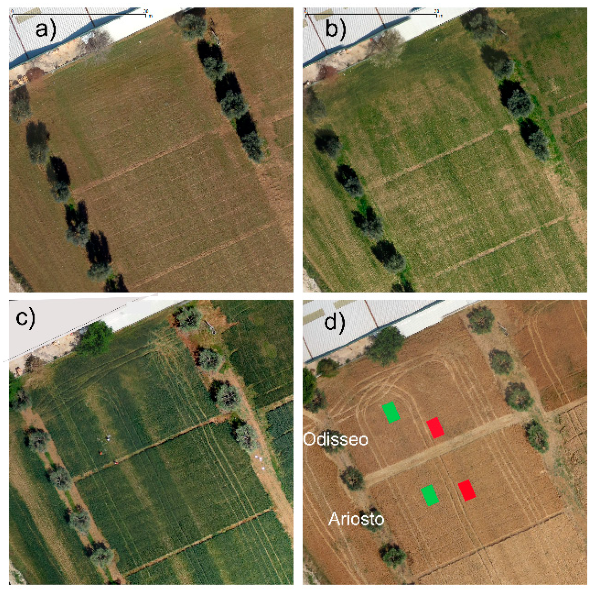
Furthermore, at harvest, within each cultivar, yield data and yield components of the whole plot (720 m²) were measured, as well as for four sub-areas, 10 m² each was characterized by the different yield levels in Figure 1 (H = high yield and L = low yield). The sub-areas were selected within the homogeneous areas detected using a hierarchical clustering method, Ward’s minimum variance approach, as reported in a previous paper for Odisseo [25] and calculated for Ariosto. NDVI and OSAVI high-resolution data of the four areas were analyzed backward in time to deliver relative frequency histograms of VI values.

2.2. UAV System and Flight Missions

Four flight missions were carried out in the same dates to measure the destructive plant samples: for seedling (February 23), tillering (March 30), anthesis (May 14), harvest (July 7), with eBee UAV (senseFly, Cheseaux-sur-Lausanne, Switzerland). The eBee, designed as a fixed-wing UAV for application in precision agriculture (payload of 150 g). All flights were carried out in stable ambient light conditions from 11:30 a.m. to 1:00 p.m., with excellent visibility and wind below 5 m s⁻¹, at a flight altitude of 97 m (A.G.L.). The imaged area of the experimental field, including the surroundings, is about 15 hectares so that 96 camera stations (single flight) and 15 min flight were needed. The autopilot analyzes (continuously) the inertial measurement unit (IMU) and onboard GPS data to control every aspect of the eBee’s flight. The integration of the UAV and sensors with GPS and IMU enables obtaining direct georeferencing imaging after image processing. At any acquisition date, two flights were carried out, the first one by a Canon Powershot S110 photo camera (visible spectrum, RGB-red/green/blue) for visible RGB image (orthophoto) to run a rapid analysis for visual crop variability. The second flight used a Canon Powershot S110 NIR camera (near infra-red, NIRGB—near infra-red/green/blue) which provides maximum absorption peaks at 550 nm (green), 625 nm (red), and 850 nm (NIR) wavelengths, respectively, allowing the computation of VIs.

The S110 RGB and S110 NIR camera characteristics were: weight 0.7 kg, resolution 12 million pixels, sensor size 5.58 × 7.44 mm², pixel pitch 1.33 μm, and format images RAW JPEG. The S110 RGB camera acquired the true-color, while the S110 NIR acquired the false-color image data at 0.55 μm (green), 0.625 μm (red), and 0.85 μm (NIR) bands.

To avoid geometric distortion due to low altitude, 96 overlapping pictures from each camera and flight were used for mosaicking to produce an ortho-image. An 80% frontal overlap and an 80% side overlap were used.

To relate and orient UAV imagery to the ground, ten ground control points (GCPs) were distributed across the field at the beginning of the season, to obtain photogrammetric imagery with uniform vertical and horizontal accuracy. The GCPs were 25 cm × 25 cm square, with a specific albedo for camera calibration (atmospheric corrections). The GCP coordinates were ensured with a Leica Viva GS15 (Leica Geosystems AG, Heerbrugg, Switzerland) GPS (horizontal accuracy of 0.025 m-vertical accuracy of 0.035 m). Fixed targets were used for a more accurate geo-referencing of UAV aerial imagery and for overlaying the measurements from multiple dates.

2.3. Data Processing

The acquired images were processed by the eMotion software (senseFly, Cheseaux-sur-Lausanne, Switzerland) to generate low-resolution visible (RGB) images of the crops. The eBee’s supplied software to build a project using the drone’s geo-tagged images. The project is loaded on a laptop in Pix4Dmapper Ag (senseFly, Cheseaux-sur-Lausanne, Switzerland) to run a rapid analysis for visual crop variability.

The multiple overlapped images of the whole plot were stitched and ortho-rectified to create the geo-referenced ortho-mosaicked image. In the laboratory, data processing (orthomosaicking) of acquired images were performed with Postflight Terra 3D software package, a customized version of the Pix4D digital photogrammetric solution specifically optimized for the eBee, to generate ortho-images. Postflight Terra 3D incorporates a scale-invariant feature transform (SIFT) algorithm to match key points across multiple images [26] and process data in three key steps: (1) initial processing, (2) point cloud densification, and (3) orthomosaic generation.

Ortho-rectification by aero-triangulation and mosaicking were elaborated for processing, starting from the exterior position and orientation parameters provided by the UAV internal system (roll, pitch, and yaw angles). Orthoimages were produced from the flights, with a pixel resolution of 5 cm. Ten GCPs (Leica Viva GS15 (Leica Geosystems AG, Heerbrugg, Switzerland) were used to complete the external camera orientation. The orthomosaic was georeferenced to UTM-WGS84 zone 33N Italy. The final outputs were an RGB (Visible) GeoTIFF with a resolution of 5 cm² pixels.

The normalized difference vegetation index (NDVI) and the soil-adjusted vegetation index (SAVI) layers were generated in a raster calculator from extracted red (R) and near infra-red (NIR) channels. The index calculator function of Postflight Terra 3D was used for generating VI maps. A certificate of calibration of Canon S110 NIR was uploaded in the software to optimize internal camera parameters, such as focal length, principal points, and lens distortions. The ten GCPs with a known albedo for Red, Green, and NIR channel (reflectance panel) were used to calibrate the camera to achieve uniform quality of image (exposure and brightness) and for atmospheric correction in the software section “processing options,” point 3 DSM, orthomosaic, index and for creating VIs map. The resolution of the reflectance map has been set at 5 cm² pixels, the whole map was elaborated for each VI and date, and the NDVI and OSAVI formula were selected (index map function). The final outputs were an NDVI GeoTIFF and an OSAVI GeoTIFF, both with a resolution of 5 cm² pixels. GeoTIFF images and georeferenced sampling data were processed for agronomic purpose with QGIS 2.8.1.

2.4. Vegetation Indices

The normalized difference vegetation index (NDVI) was calculated according to Equation (1):

NDVI = (NIR − RED)/(NIR + RED)

(1)

The NDVI ranges from −1.0 to 1.0, where positive values indicate increasing greenness and negative values indicate non-vegetated features. It has some disadvantages though such as saturation in later growth stages [27,28].

The optimized soil-adjusted vegetation index (OSAVI) was calculated according to Equation (2). The OSAVI index was proposed by Rondeaux et al. [29] using reflectance in the red and near-infrared bands; through the following formulation:

OSAVI = (NIR − RED)/(NIR + RED + 0.16)

(2)

where 0.16 is the soil adjustment coefficient, selected according to the optimal value to minimize soil background variations.

2.5. Statistical Analysis

Regression analysis, coefficients of determination, significance levels, and RMSE were computed on two sets of geo-referred data: ground crop samplings (LAI, Biomass, and spikes for square meter) and remote UAV data using the statistical package Origin PRO 8 (Origin Lab Corporation, Northampton, MA, USA). H and L sub-area were selected starting from homogeneous areas identified in a previous paper [22] as follow: the yield-related traits and VIs data were analyzed using the hierarchical clustering Ward’s minimum variance approach [30] to classify observations into groups, in which the group members have common properties. Statistical procedures were computed using OriginPRO 8. The difference between H and L sub-areas were recorded by the analysis of variance.

3. Results and Discussion

Ground agronomic data (biomass, green leaf area index, spikes, and plant height) of each cultivar have been correlated to high-resolution multispectral images (NDVI and OSAVI). The correlation of the whole crop cycle data was performed in accordance with van Ittersum et al. [31], who states that it is essential to study the relationship among VIs and crop traits, to evaluate and estimate the yield potential and the yield gap (

Table 1. Polynomial regression analysis of vegetation index (VI) data and crop parameters each based on 44 data points. LAI = leaf area index, RMSE = root mean square error. Significance level: p-value < 0.001.

	Odisseo				Ariosto
	NDVI		OSAVI		NDVI		OSAVI
	R2	RMSE	R2	RMSE	R2	RMSE	R2	RMSE
Biomass	0.953	0.06	0.943	0.062	0.859	0.075	0.857	0.082
LAI	0.910	0.059	0.879	0.076	0.777	0.095	0.763	0.106
Spikes	0.788	0.067	0.790	0.075	0.769	0.042	0.597	0.065
Height	0.828	0.083	0.817	0.102	0.518	0.105	0.519	0.127

). In the present study, polynomial regressions were found to be the simplest adjustment to report the time-course variability along the growth stage, starting from seedling to harvest. Moreover, significant relationships with different R² values were found for both the indices and crop growth traits. The spectro-radiometric response of the wheat canopy was not linear during the growing period in accordance with Aparicio et al. [32] and Dang et al. [33], since the high sensitivity of the VIs when LAI is lower (early season) and less sensitive after the canopy closes.

The relationships among VIs and crop parameters were highly significant: the R² for NDVI vs. biomass reached 0.953 for Odisseo and 0.859 for Ariosto, while the R² of OSAVI vs. biomass was 0.943 for Odisseo and 0.857 for Ariosto. The relationships among each VI and LAI showed an R² of 0.910 for NDVI Odisseo and R² of 0.777 for Ariosto, and it was 0.879 for OSAVI Odisseo and 0.763 for Ariosto. The relationships among each VI and height showed an R² of 0.828 for NDVI Odisseo and 0.817 for OSAVI Odisseo and R² of 0.518 for both NDVI and OSAVI for Ariosto. Ground truth georeferenced data of the number of spikes per square meter at harvest stages were also related to NDVI and OSAVI data; significant relationships were found with an R² of 0.788 for Odisseo and 0.769 for Ariosto recorded for NDVI index and an R² of 0.790 for Odisseo and of 0.597 for Ariosto recorded for OSAVI index.

Briefly, all R² of yield components were highly correlated (p-value < 0.001) with VIs, and are higher for Odisseo than the Ariosto.

3.1. Agronomic Data and VIs at Different Crop Growth Stages

In the whole plot, the biomass at seedling stage ranged from 68 to 156 g m⁻² for both cultivars and that of LAI (0.12 to 0.47) (

Table 2. Range value (min and max), mean and standard deviation (SD) of yield components (biomass, LAI, plant height, and spike) and vegetation indices (VIs) (NDVI and OSAVI) measured at seedling, tillering, and anthesis stages.

Growth Stages	Yield Components and VIs	Odisseo				Ariosto
		Min	Max	Mean	SD	Min	Max	Mean	SD
Seedling	Biomass (g m−2)	72.2	156.1	102.1	30.0	67.5	145.0	97.8	26.6
	LAI	0.167	0.472	0.267	0.086	0.123	0.424	0.269	0.089
	NDVI	0.266	0.467	0.383	0.083	0.263	0.569	0.414	0.098
	OSAVI	0.386	0.596	0.499	0.087	0.381	0.650	0.532	0.088
Tillering	Biomass (g m−2)	116	558	332	149	185.2	740.8	363.05	185.9
	LAI	0.328	1.610	0.922	0.409	0.500	2.259	1.106	0.566
	Plant height (cm)	34.5	54.5	45.8	5.43	28.3	45.6	39.1	5.2
	NDVI	0.338	0.828	0.639	0.165	0.434	0.857	0.637	0.145
	OSAVI	0.400	0.978	0.755	0.195	0.500	0.991	0.743	0.166
Anthesis	Biomass (g m−2)	282	1116	761	258	587.5	1453.9	911.5	251.6
	LAI	0.732	2.56	1.722	0.546	1.32	2.69	1.94	0.459
	Spikes (n° m−2)	217	527	411	91	258	651	415	119
	Plant height (cm)	39.0	73.0	63.2	10.7	60.0	73.0	69.5	3.9
	NDVI	0.527	0.838	0.753	0.092	0.654	0.876	0.814	0.073
	OSAVI	0.631	1.004	0.892	0.112	0.725	1.067	0.955	0.105

), while VIs ranged from 0.26 to 0.57 for NDVI and from 0.38 to 0.65 for OSAVI, for both cultivars. The light differences recorded within yield components as well as VIs value gave no significant relationships among VIs and yield components (

Table 3. Polynomial regression analysis of VIs data and crop parameters (whole plots) during crop cycle (seedling, tillering, and anthesis). LAI = leaf area index, RMSE = root mean square error, n.s. = not significant.

Growth Stages	VIs	Yield Components	Odisseo			Ariosto
			R2	RMSE	p-Value	R2	RMSE	p-Value
Seedling	NDVI	Biomass	n.s.	0.0588	0.039	n.s.	0.082	0.012
		LAI	n.s.	0.0577	0.034	n.s.	0.079	0.097
	OSAVI	Biomass	n.s.	0.5175	0.032	n.s.	0.071	0.092
		LAI	n.s.	0.0684	0.079	n.s.	0.076	0.144
Tillering	NDVI	Biomass	0.882	0.063	0.001	0.665	0.077	0.007
		LAI	0.852	0.070	0.001	0.689	0.089	0.005
		Plant height	0.866	0.091	0.002	n.s.	0.141	0.320
	OSAVI	Biomass	0.937	0.851	0.001	0.672	0.105	0.007
		LAI	0.844	0.085	0.001	0.687	0.103	0.005
		Plant height	0.859	0.110	0.002	n.s.	0.16	0.250
Anthesis	NDVI	Biomass	0.893	0.033	0.001	0.818	0.007	0.001
		LAI	0.843	0.040	0.001	0.694	0.073	0.422
		Spikes	0.725	0.060	0.001	0.768	0.044	0.001
		Plant height	0.736	0.070	0.030	0.820	0.046	0.010
	OSAVI	Biomass	0.804	0.756	0.001	0.777	0.055	0.002
		LAI	0.745	0.063	0.002	0.672	0.106	0.470
		Spikes	0.680	0.074	0.008	0.697	0.060	0.001
		Plant height	0.680	0.091	0.061	0.803	0.070	0.016

). This was due to a low amount of accumulated biomass and LAI values, as well as the difficulties of simple indices to discriminate between soil and vegetation as found also by many authors, such as Aparicio et al. [34] and Chlingaryan et al. [24].

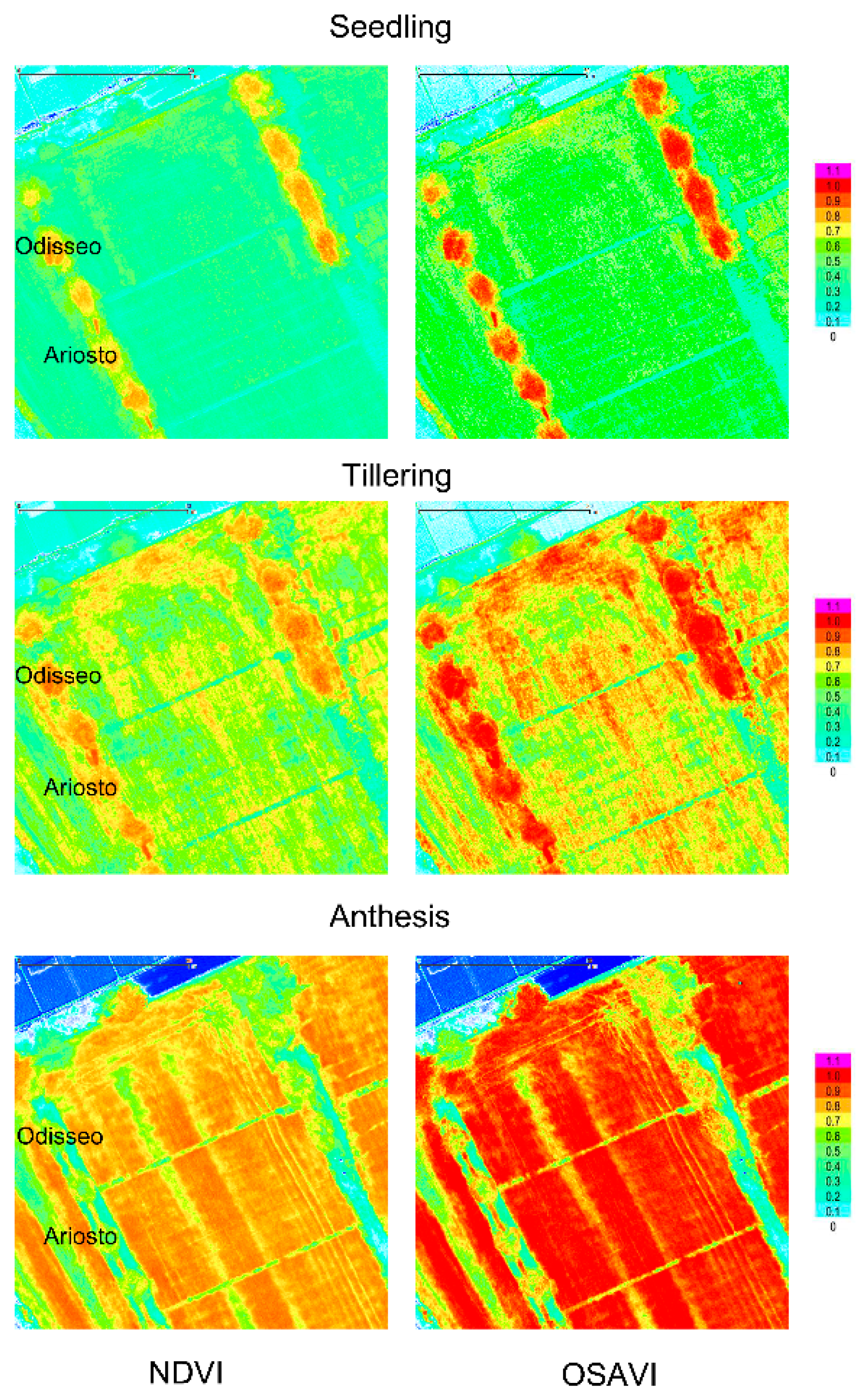
At the tillering stage, the spatial variability of crop traits was highly evident; thus, the most productive data was shown by the biomass and LAI which was four times higher than the less favored zones (Table 2).

In the most productive zones, VI values ranged from 0.85 to 0.99 (for both cultivars), which revealed 2.5 times more than the lower value (Figure 2).

The relationships between VIs and crop parameters were highly significant for both cultivars (Table 3). For biomass, the R² reached 0.88 for Odisseo and 0.66 for Ariosto for LAI, the R² reached 0.85 for Odisseo and 0.69 for Ariosto. The plant height and VI regression were not significant for Ariosto. These results are in accordance with findings of several authors at tillering, for example Dalla Marta et al. [35] found a highly significant (positive) relationship with biomass weight, while Reyniers and Vrindts [36] and Magney et al. [37] found respectively an R² of 0.76 and R² = 0.62 between NDVI and biomass.

At anthesis, the high spatial variability of the crop traits value and VI values were still evident for both cultivars (Table 2, Figure 2). VIs were highly correlated to crop traits as reported in Table 3; the values of the R² for NDVI vs. biomass reached 0.89 for Odisseo and 0.82 for Ariosto, while the R² of OSAVI vs. biomass was 0.80 for Odisseo and 0.78 for Ariosto (p < 0.001).

These results are in accordance with the Marti et al. [38], who found the highest correlation values between growth and NDVI measurements when performed around anthesis, such as with Villegas et al. [39] that reported the highest values of R² for the relationship between NDVI and crop dry weight at anthesis. Cabrera-Bosquet et al. [40] have demonstrated a strong linear regression between durum wheat and VIs. On the contrary, Dalla Marta et al. [35] found completely different results, with no correlations observed between the crop parameters and the indices, due to VIs saturation.

3.2. Backward Analysis

Table 4. Yield (t ha⁻¹), biomass (g m⁻²), spike number (n° m⁻²), and plant height (cm) of Odisseo and Ariosto at harvest stage. Mean data are related to the whole plot (W) and to the sub-areas; H_o (high yield of Odisseo) and H_A (high yield of Ariosto), L_O (low yield Odisseo), and L_A (low yield Ariosto). The p-level values are related to H and L significant differences within each cultivar.

	Odisseo				Ariosto
	W	HO (SD)	LO (SD)	p-level	W	HA (SD)	LA (SD)	p-level
Yield (t ha−1)	5.73	6.77 (0.83)	4.66 (0.61)	<0.0064	5.05	6.17 (0.44)	3.94 (0.25)	1.26 × 10−4
Biomass (g m−2)	760	1029 (106)	500 (208)	<0.0398	911	1171 (200)	682 (77)	<0.0039
Spikes (n° m−2)	412	509 (74.3)	320 (27.3)	<0.0034	360	465 (25)	230 (31)	2.39 × 10−5
Plant height (cm)	63.2	72.2 (2.95)	50.5 (8.5)	<0.0236	69.5	72.5 (5.57)	66.25 (4.78)	n.s.

reports yield and yield components at harvest for the complete plot (W), as well as data of the two sub-areas, H_O and H_A with high yield and L_O and L_A with low yield.

The yield data of both cultivars were in accordance with those reported by Visioli et al. [41] in Italy. The crop yield of the whole plots was 5.73 t ha⁻¹ for Odisseo (W_O) and 5.05 t ha⁻¹ for Ariosto (W_A). The yield of H_O and H_A were about 20% higher than the whole plot yield, which in turn were 20% higher than L_O and L_A. Yield components were ranked according to the yield levels: biomass and spikes per square meter of H were about 25–35% higher than the W and 37–50% higher than L sub-plot areas_. Differences in plant heights were less marked.

The subplot detected at harvest was analyzed backward in time from anthesis to seedling.

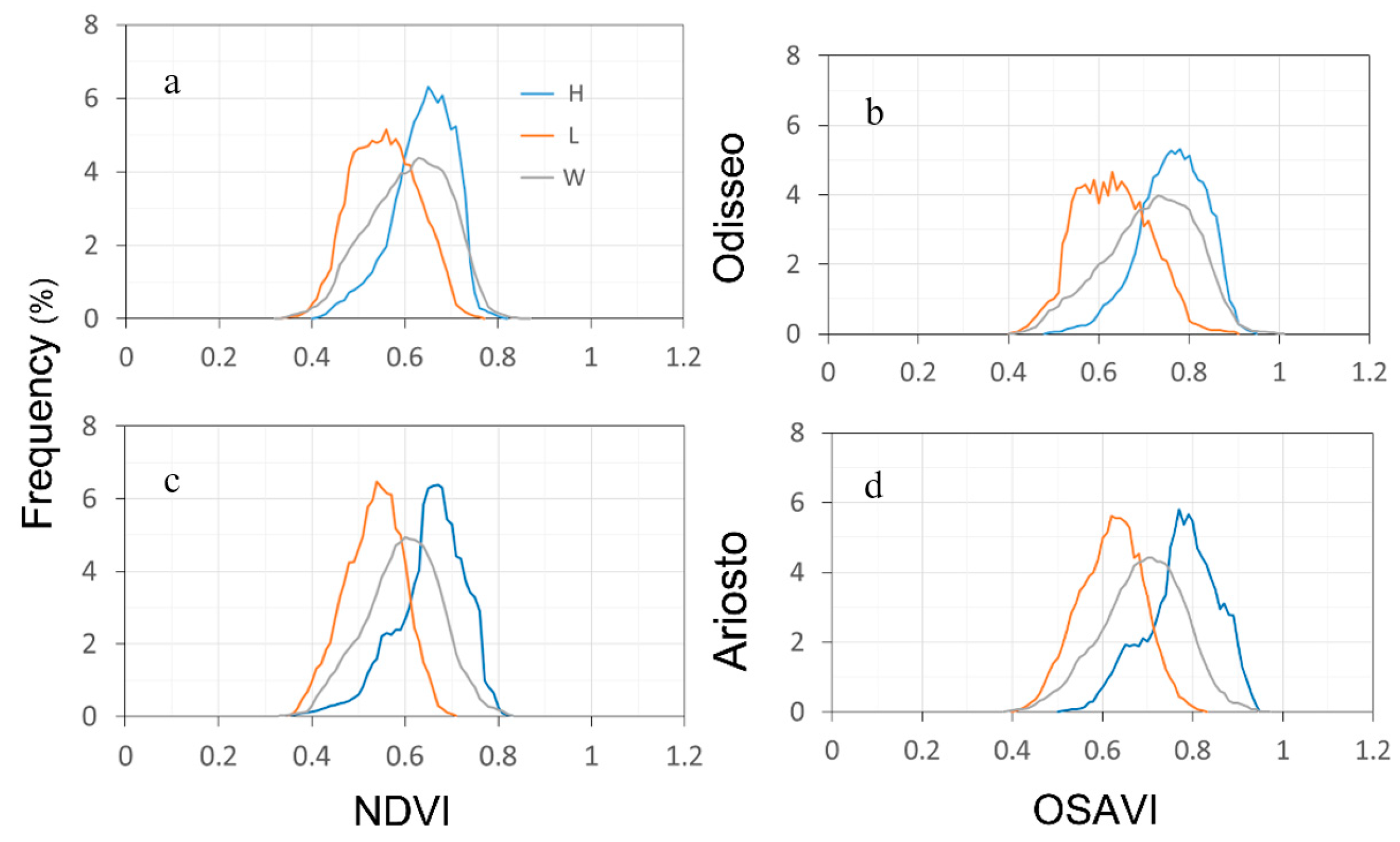
At anthesis, the analysis of VI value frequencies showed the maximum evidence of different crop status of H and L sub-areas and W plots. More than the 75% of the surface of the sub-areas showed a value higher (H sub-plot) or lower (L sub-plot) than W plot (Figure 3). The H and L areas curves showed a low overlapping. The H curve appeared narrow and tall. Data were confirmed by all the yield components that were significantly different from each other in the two sub-areas and W plot.

At tillering, the histogram of VIs frequency (Figure 4) shows differences among the whole plot data, both H and L areas. These differences were lower than those detected at the anthesis stage.

For both the cultivars and indices, the H zones showed values of the frequency which were higher than the 75% of H_O and H_A, and L_A, L_O VI values were higher and lower respectively than the median value of the whole plot.

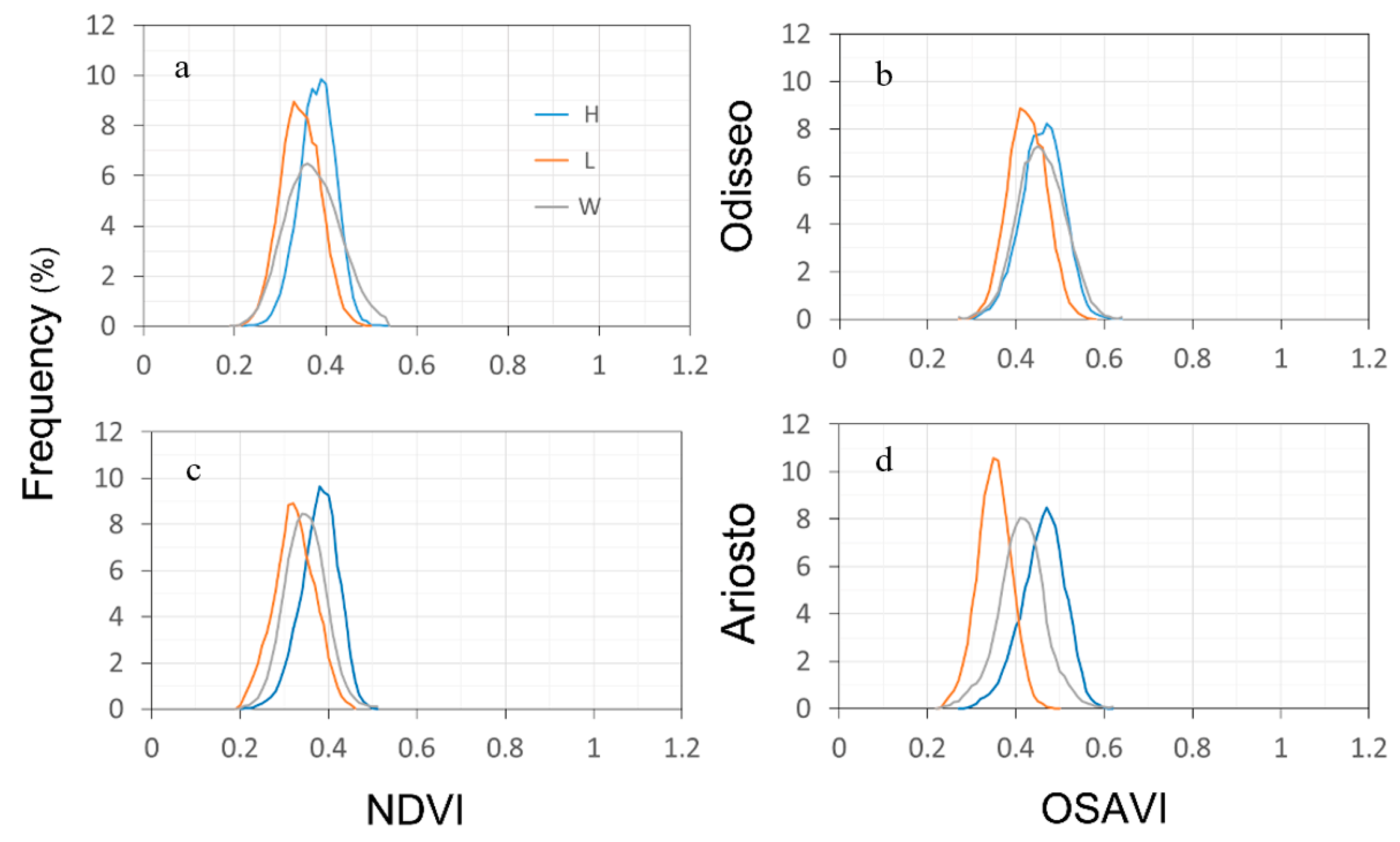
At the seedling stage, the relative frequency curves of the two VIs are presented in Figure 5. In all the graphs, the curves appeared to be very close, except for the OSAVI of Ariosto (d) at the seedling stage.

In all graphs, about 75% of the H data (third percentile) were higher than the second percentile of the W curve as well as the first percentile of L data. The highest differences between H and L curves were detected for the OSAVI index, Ariosto (d), because the index that considers soil brightness are perform slightly better than the NDVI, as reported in different studies [42,43].

4. Conclusions

In the last few years, UAVs have been used as tools that provide a high number of information per square meter for precision agriculture management and its development. The potentials of the information provided by the drone images have not yet been fully explored. In this paper, we have analyzed the frequency distribution curves of high-resolution VIs images of the two cultivars of durum wheat.

Within each cultivar, two yield sub-areas were detected by cluster analysis at the harvest stage and analyzed backward at different growth stages, in comparison with the whole plot data. The crop yield of the whole plots revealed 5.73 t ha⁻¹ for Odisseo (W_O) and 5.05 t ha⁻¹ for Ariosto (W_A). The yield for H_O and H_A recorded 20% higher than the whole plot yield, which in turn were 20% higher than L_O and L_A, moreover the biomass and the spikes per square meter of H was noted 25–35% higher than the W and 37–50% higher than L sub-plot areas, confirming the ability of cluster analysis to detect groups with the same variability.

The analysis of frequencies of high-resolution VI images showed that the 75% of H data (third percentile) were recorded higher than the second percentile of the W curve as well as for the first percentile of L data. The maximum evidence of different crop status of H and L sub-areas and W plots were detected at anthesis by both indices and cultivars.

The analysis of frequency curves provided significant differences at the seedling stage where agronomic parameters showed only slight differences which were revealed as not significant following the traditional approach (regression between agronomic traits and VIs). For Ariosto, the seedling OSAVI index showed an interesting differentiation among areas, confirming the ability of OSAVI to consider the soil brightness.

The analysis of frequencies of high-resolution VI images provided detailed information on crop spatial and temporal variability and can allow developing a new approach for automatic detection of suitable vegetation indices, and spatial and temporal crop variability for precision agriculture practices.

References

- Cavallo, G.; De Benedetto, D.; Castrignanò, A.; Quarto, R.; Vonella, A.V.; Buttafuoco, G. Use of geophysical data for assessing 3D soil variation in a durum wheat field and their association with crop yield. Biosyst. Eng. 2016, 152, 28–40. [Google Scholar] [CrossRef]
- Zhang, C.; Kovacs, J.M. The application of small unmanned aerial systems for precision agriculture: A review. Precis. Agric. 2012, 13, 693–712. [Google Scholar] [CrossRef]
- Candiago, S.; Remondino, F.; De Giglio, M.; Dubbini, M.; Gattelli, M. Evaluating multispectral images and vegetation indices for precision farming applications from UAV images. Remote Sens. 2015, 7, 4026–4047. [Google Scholar] [CrossRef]
- Guo, L.; An, N.; Wang, K. Reconciling the discrepancy in ground- and satellite-observed trends in the spring phenology of winter wheat in China from 1993 to 2008. J. Geophys. Res. Atmos. 2016, 121, 1027–1042. [Google Scholar] [CrossRef] [Green Version]
- Schirrmann, M.; Giebel, A.; Gleiniger, F.; Pflanz, M.; Lentschke, J.; Dammer, K.H. Monitoring Agronomic Parameters of Winter Wheat Crops with Low-Cost UAV Imagery. Remote Sens. 2016, 8, 706. [Google Scholar] [CrossRef]
- Rasmussen, J.; Ntakos, G.; Nielsen, J.; Svensgaard, J.; Poulsen, R.N.; Christensen, S. Are vegetation indices derived from consumer-grade cameras mounted on UAVs sufficiently reliable for assessing experimental plots? Eur. J. Agron. 2016, 74, 75–92. [Google Scholar] [CrossRef]
- Duan, T.; Chapman, S.C.; Guo, Y.; Zheng, B. Dynamic monitoring of NDVI in wheat agronomy and breeding trials using an unmanned aerial vehicle. F. Crop. Res. 2017, 210, 71–80. [Google Scholar] [CrossRef]
- Abdollahnejad, A.; Panagiotidis, D.; Surový, P.; Ulbrichová, I. UAV capability to detect and interpret solar radiation as a potential replacement method to hemispherical photography. Remote Sens. 2018, 10, 423. [Google Scholar] [CrossRef]
- Alvino, A.; Marino, S.; Alvino, A.; Marino, S. Remote Sensing for Irrigation of Horticultural Crops. Horticulturae 2017, 3, 40. [Google Scholar] [CrossRef]
- Mulla, D.J. Twenty five years of remote sensing in precision agriculture: Key advances and remaining knowledge gaps. Biosyst. Eng. 2013, 114, 358–371. [Google Scholar] [CrossRef]
- Kyratzis, A.C.; Skarlatos, D.P.; Menexes, G.C.; Vamvakousis, V.F.; Katsiotis, A. Assessment of Vegetation Indices Derived by UAV Imagery for Durum Wheat Phenotyping under a Water Limited and Heat Stressed Mediterranean Environment. Front. Plant Sci. 2017, 8, 1–14. [Google Scholar] [CrossRef] [PubMed]
- Liebisch, F.; Kirchgessner, N.; Schneider, D.; Walter, A.; Hund, A. Remote, aerial phenotyping of maize traits with a mobile multi-sensor approach. Plant Methods 2015, 11. [Google Scholar] [CrossRef] [PubMed]
- Basso, B.; Cammarano, D.; Cafiero, G.; Marino, S.; Alvino, A. Cultivar discrimination at different site elevations with remotely sensed vegetation indices. Ital. J. Agron. 2011, 6, 1–5. [Google Scholar] [CrossRef]
- Marino, S.; Alvino, A. Proximal sensing and vegetation indices for site-specific evaluation on an irrigated crop tomato. Eur. J. Remote Sens. 2014, 47, 271–283. [Google Scholar] [CrossRef] [Green Version]
- Marino, S.; Aria, M.; Basso, B.; Leone, A.P.; Alvino, A. Use of soil and vegetation spectroradiometry to investigate crop water use efficiency of a drip irrigated tomato. Eur. J. Agron. 2014, 59, 67–77. [Google Scholar] [CrossRef]
- Marino, S.; Cocozza, C.; Tognetti, R.; Alvino, A. Use of proximal sensing and vegetation indexes to detect the inefficient spatial allocation of drip irrigation in a spot area of tomato field crop. Precision Agric. 2015, 16, 613–629. [Google Scholar] [CrossRef]
- Yue, J.; Feng, H.; Jin, X.; Yuan, H.; Li, Z.; Zhou, C.; Yang, G.; Tian, Q. A comparison of crop parameters estimation using images from UAV-Mounted Snapshot Hyperspectral Sensor and High-Definition Digital Camera. Remote Sens. 2018, 10, 1138. [Google Scholar] [CrossRef]
- Holman, F.H.; Riche, A.B.; Michalski, A.; Castle, M.; Wooster, M.J.; Hawkesford, M.J. High throughput field phenotyping of wheat plant height and growth rate in field plot trials using UAV based remote sensing. Remote Sens. 2016, 8. [Google Scholar] [CrossRef]
- Araus, J.L.; Cairns, J.E. Field high-throughput phenotyping: The new crop breeding frontier. Trends Plant Sci. 2014, 19, 52–61. [Google Scholar] [CrossRef] [PubMed]
- Erdle, K.; Mistele, B.; Schmidhalter, U. Spectral high-throughput assessments of phenotypic differences in biomass and nitrogen partitioning during grain filling of wheat under high yielding Western European conditions. F. Crop. Res. 2013, 141, 16–26. [Google Scholar] [CrossRef]
- Fischer, R.A. Wheat physiology: A review of recent developments. Crop Pasture Sci. 2011, 62, 95–114. [Google Scholar] [CrossRef]
- Marino, S.; Alvino, A. Detection of homogeneous wheat areas using multi-temporal UAS images and ground truth data analyzed by cluster analysis. Eur. J. Remote Sens. 2018, 51, 266–275. [Google Scholar] [CrossRef]
- Damian, J.M.; De Castro Pias, O.H.; Santi, A.L.; Di Virgilio, N.; Berghetti, J.; Barbanti, L.; Martelli, R. Delineating management zones for precision agriculture applications: A case study on wheat in sub-tropical Brazil. Ital. J. Agron. 2016, 11, 171–179. [Google Scholar] [CrossRef]
- Chlingaryan, A.; Sukkarieh, S.; Whelan, B. Machine learning approaches for crop yield prediction and nitrogen status estimation in precision agriculture: A review. Comput. Electron. Agric. 2018, 151, 61–69. [Google Scholar] [CrossRef]
- Zadoks, J.C.; Chang, T.T.; Konzak, C.F. A decimal code for the growth stages of cereals. Weed Res. 1974, 14, 415–421. [Google Scholar] [CrossRef]
- Küng, O.; Strecha, C.; Beyeler, A.; Zufferey, J.-C.; Floreano, D.; Fua, P.; Gervaix, F. The accuracy of automatic photogrammetric technique on ultra-light UAV imagery. Int. Arch. Photogramm. Remote Sens. Spat. Inf. Sci. 2012, XXXVIII-1/C22, 125–130. [Google Scholar] [CrossRef]
- Lopresti, M.F.; Di Bella, C.M.; Degioanni, A.J. Relationship between MODIS-NDVI data and wheatyield: A case study in Northern Buenos Airesprovince, Argentina. Inf. Process. Agric. 2015, 2, 73–84. [Google Scholar] [CrossRef]
- Colomina, I.; Molina, P. Unmanned aerial systems for photogrammetry and remote sensing: A review. ISPRS J. Photogramm. Remote Sens. 2014, 92, 79–97. [Google Scholar] [CrossRef] [Green Version]
- Rondeaux, G.; Steven, M.; Baret, F. Optimization of soil-adjusted vegetation indices. Remote Sens. Environ. 1996, 55, 95–107. [Google Scholar] [CrossRef]
- Ward, J.H. Hierarchical Grouping to Optimize an Objective Function. J. Am. Stat. Assoc. 1963, 58, 236–244. [Google Scholar] [CrossRef] [Green Version]
- Van Ittersum, M.K.; Cassman, K.G.; Grassini, P.; Wolf, J.; Tittonell, P.; Hochman, Z. Yield gap analysis with local to global relevance—A review. Field Crop. Res. 2013, 143, 4–17. [Google Scholar] [CrossRef] [Green Version]
- Aparicio, N.; Villegas, D.; Casadesus, J.; Araus, J.L.; Royo, C. Spectral Vegetation Indices as Nondestructive Tools for Determining Durum Wheat Yield. Agron. J. 2000, 92, 83–91. [Google Scholar] [CrossRef]
- Dang, Y.P.; Pringle, M.J.; Schmidt, M.; Dalal, R.C.; Apan, A. Identifying the spatial variability of soil constraints using multi-year remote sensing. F. Crop. Res. 2011, 123, 248–258. [Google Scholar] [CrossRef]
- Aparicio, N.; Villegas, D.; Royo, C.; Casadesus, J.; Araus, J.L. Effect of sensor view angle on the assessment of agronomic traits by ground level hyper-spectral reflectance measurements in durum wheat under contrasting Mediterranean conditions. Int. J. Remote Sens. 2004, 25, 1131–1152. [Google Scholar] [CrossRef]
- Dalla Marta, A.; Grifoni, D.; Mancini, M.; Orlando, F.; Guasconi, F.; Orlandini, S. Durum wheat in-field monitoring and early-yield prediction: Assessment of potential use of high resolution satellite imagery in a hilly area of Tuscany, Central Italy. J. Agric. Sci. 2015, 153, 68–77. [Google Scholar] [CrossRef]
- Reyniers, M.; Vrindts, E. Measuring wheat nitrogen status from space and ground-based platform. Int. J. Remote Sens. 2006, 27, 549–567. [Google Scholar] [CrossRef]
- Magney, T.S.; Eitel, J.U.H.; Huggins, D.R.; Vierling, L.A. Proximal NDVI derived phenology improves in-season predictions of wheat quantity and quality. Agric. For. Meteorol. 2016, 217, 46–60. [Google Scholar] [CrossRef]
- Marti, J.; Bort, J.; Slafer, G.A.; Araus, J.L. Can wheat yield be assessed by early measurements of Normalized Difference Vegetation Index? Ann. Appl. Biol. 2007, 150, 253–257. [Google Scholar] [CrossRef]
- Villegas, D.; Aparicio, N.; Blanco, R.; Royo, C. Biomass accumulation and main stem elongation of Durum wheat grown under Mediterranean conditions. Ann. Bot. 2001, 88, 617–627. [Google Scholar] [CrossRef]
- Cabrera-Bosquet, L.; Molero, G.; Stellacci, A.; Bort, J.; Nogués, S.; Araus, J. NDVI as a potential tool for predicting biomass, plant nitrogen content and growth in wheat genotypes subjected to different water and nitrogen conditions. Cereal Res. Commun. 2011, 39, 147–159. [Google Scholar] [CrossRef]
- Visioli, G.; Bonas, U.; Dal Cortivo, C.; Pasini, G.; Marmiroli, N.; Mosca, G.; Vamerali, T. Variations in yield and gluten proteins in durum wheat varieties under late-season foliar versus soil application of nitrogen fertilizer in a northern Mediterranean environment. J. Sci. Food Agric. 2018, 98, 2360–2369. [Google Scholar] [CrossRef] [PubMed]
- Marino, S.; Alvino, A. Hyperspectral vegetation indices for predicting onion (Allium cepa L.) yield spatial variability. Comput. Electron. Agric. 2015, 116. [Google Scholar] [CrossRef]
- Marino, S.; Basso, B.; Leone, A.P.; Alvino, A. Agronomic traits and vegetation indices of two onion hybrids. Sci. Hortic. 2013, 155, 56–64. [Google Scholar] [CrossRef]
Figure 1.
RGB images and samplings H (red) and L (green) areas of Odisseo (above) and Ariosto (below) at seedling (a), tillering (b), anthesis (c), and harvest (d) stages.
Figure 2.
Normalized difference vegetation index (NDVI) and optimized soil-adjusted vegetation index (OSAVI) images for Odisseo (upper plot) and Ariosto (lower plot), at seedling, tillering, and anthesis growth stages.
Figure 3.
Relative frequency curves of the two VIs, NDVI (a–c) and OSAVI (b–d) within each cultivar, Odisseo (a–b) and Ariosto (c–d). In grey, the whole plot (W) curves have been shown, in red the low-yield sub-areas (L), and in blue the high-yield sub-areas (H) at the anthesis stage.
Figure 4.
Relative frequency curves of the two VIs, NDVI (a–c) and OSAVI (b–d) within each cultivar, Odisseo (a–b) and Ariosto (c–d). In grey, the whole plot (W) curves have been shown, in red the low-yield sub-areas (L), and in blue the high-yield sub-areas (H) at the tillering stage.
Figure 5.
Relative frequency curves of the two VIs, NDVI (a–c) and OSAVI (b–d) within each cultivar, Odisseo (a–b) and Ariosto (c–d). In grey, the whole plot (W) curves have been shown, in red the low-yield sub-areas (L), and in blue the high-yield sub-areas (H) at the seedling stage.