Different Paths for Developing Terrestrial LiDAR Data for Comparative Analyses of Topographic Surface Changes


Institute of Earth and Environmental Sciences, Faculty of Earth Sciences and Spatial Management, Maria Curie-Sklodowska University in Lublin, Al. Krasnicka 2 D, 20-718 Lublin, Poland
Appl. Sci. 2020, 10(21), 7409; https://0-doi-org.brum.beds.ac.uk/10.3390/app10217409
Submission received: 16 September 2020
/
Revised: 12 October 2020
/
Accepted: 20 October 2020
/
Published: 22 October 2020
(This article belongs to the Special Issue Sustainable Use of Natural Resources)
Abstract
:High resolution terrestrial laser scanning data (TLS; terrestrial LiDAR) provide an excellent background for quantitative resource estimation through the comparative analysis of topographic surface changes. However, unlike airborne LiDAR data, which is usually provided as classified and contains a class of ground points, raw TLS data include all of the points of the scanned space within the specified scanner range. In effect, utilizing the latter data to estimate the volume of the resource by the differential analysis of digital elevation models (DEMs) requires the data to be specially prepared, i.e., separating from the point cloud only the data that represent the relevant class. In the case of natural resources, e.g., mineral resources, the class is represented by ground points. This paper presents the results that were obtained by differential analysis of high resolution DEMs (DEM of difference (DoD) method) using TLS data that were processed both manually (operator noise removal) and with the use of the automatic Cloth Simulation Filter (CSF) algorithm. Three different time pairs of DoD data were analyzed for a potential gravel-cobble deposit area of 45,444 m2, which was located at the bottom of the mouth section of the Scott River in south-east Svalbard. It was found that the applied method of ground point classification had very little influence on the errors in the range of estimating volumetric parameters of the mineral resources and measurement uncertainty. Moreover, it was shown that the point cloud density had an influence on the CSF filtering efficiency and spatial distribution of errors.
1. Introduction
High resolution LiDAR surveys have been used as basic data for the inventorying of both natural and man-made resources since the 1990s [1]. The obtained point clouds (PCs) are an accurate, unscaled representation of the scanned space [2]. The way they are used and their usefulness depend on the source, the data [3,4] and their resolution [1]. Point clouds that are obtained from airborne laser scanning (ALS) with densities ranging from a few to several dozen points per square meter (pt/m2) and with an accuracy of about 0.3–0.1 m [5] are normally used to inventory huge spaces as well as high-volume resources such as open pit mines, post-extraction heaps [6], railway or road embankments [7,8,9], landslide investigation [10] and various land cover features [11].
On the contrary, data from terrestrial laser scanning (TLS) with densities that range from several dozen to several hundred or even several thousand pt/m2 are used to inventory larger-scale resources such as quarries, gravel pits, sandpits [12] and areas that do not exceed 1 km2 [3,4]. High resolution TLS data can be used to estimate the volume of mineral deposits in order to determine the quantitative potential. The estimation of the resources’ cubic capacity (e.g., gravel or sand deposits) not only allows for assessing the economic viability of their exploitation or selecting the appropriate type of transport, but also planning the best course of action aimed at the revitalization of post-mining areas.
Repeat surveys are conducted with the intent of controlling for changes at the assumed time intervals in long-term investments as well as natural processes of geomorphic character such as erosion or deposition, which are extended in time. Such data sets, processed into digital elevation models (DEMs), make it possible to get accurate estimations of both changes in the altitude of the topographic surface and the volume in the assumed surface area where estimating the latter occurs indirectly. One of the methods of DEM differentiation at various time intervals was developed by Wheaton [13], which is the DEM of difference (DoD). Comparative studies using the DoD were used for the volumetric estimation of erosion and deposition as well as changes in the position of the topographic surface, e.g., [14,15,16,17,18].
In this method, the accuracy of estimating changes in the surface and thus the loss or increase in the resource depends on the accuracy of extracting from the raw point cloud only those points that represent the ground point [19]. On the one hand, generally available ALS data are usually provided as classified in accordance with the American Society for Photogrammetry and Remote Sensing (ASPRS) Standard LIDAR Point Classes [20] among which ground points are separated into class 2: Ground [20]. On the other hand, TLS data are usually obtained as raw and unclassified. It is in the case of the aforementioned data that the extraction of ground points from the entire cloud still poses a challenge and remains a process with a high risk of error [21]. The highest accuracy of classification is achieved by manual point cloud cleaning of all off-ground objects. However, this is an extremely time-consuming and tedious process, which can account for up to 80% of the time in the DEM development process [22,23]. Despite the widespread use of LiDAR data for DEM creation and the development of software that supports mass point cloud (PC) data processing, the classification process has proved to be extremely difficult to automate [24]. Large data sets of areas with varied land cover have proven to be a particular problem. Recently published works provide information on new generally available algorithms classifying PCs, which enable the separation of ground points, e.g., developed for the American Forestry Service (Fusion) [25], the Simple Morphological Filter [26], the Multilevel Adaptive Filter (MAF) [27] and the Cloth Simulation Filter (CSF) [28]. For noise removal from high resolution digital surface models (DSMs), deep learning methods are also applied, e.g., to sensitive filtering of raw surface elevation data or to effectively increase the automation of the segmentation process [29,30]. The CSF also handles the classification of TLS data relatively well [31]. Consequently, the accuracy of the quantitative estimation of the resource based on LiDAR data depends on the uncertainty range, which, in turn, is connected to survey errors and classification errors. The first group (survey errors) includes the range of accuracy of the measuring devices (scanner rangefinder) and positioning devices (GPS/GNSS, total station, etc.) as well as the accuracy of point cloud integration and georeferencing. While the first group includes among its input parameters the DoD for estimating the range of the measurement uncertainty, it does usually omit the accuracy of the ground point classification.
The aim and novelty of this study is therefore to answer the question as to what extent the ground point classification method affects the estimation of the quantitative parameters of mineral resources. For this purpose, an analysis was carried out on three collections of PC data sets that were obtained by utilizing one type of laser scanner at different time periods in a single area (area of interest (AoI)) whose surface was subject to significant changes during the survey’s three-year period. The classification of the ground points in this data was performed manually whilst using the CSF algorithm to obtain three sets of data to compare the range of measurement uncertainty.
2. Materials and Methods
2.1. Study Area
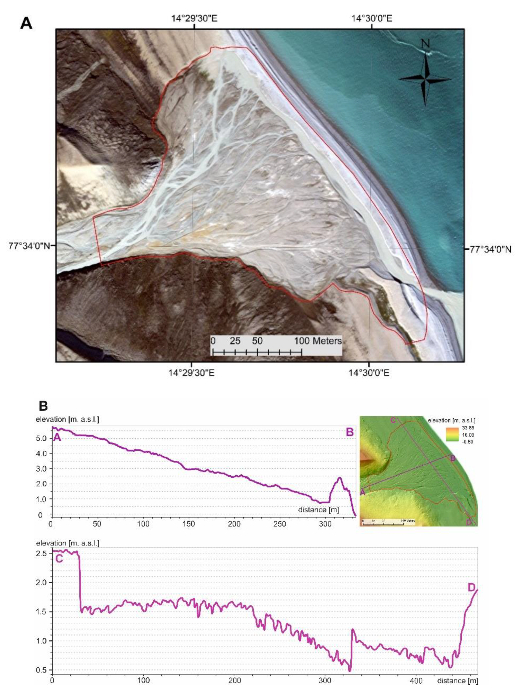
The study was carried out in the mouth section of the gravel-cobble Scott River valley floor located in the north-west part of Wedel Jarlsberg Land (south-west Svalbard, 80 km apart from the capital Longyearbyen) in the northern part of Sør-Spitsbergen National Park where 65% of the area is covered by glaciers. The Scottbreen valley glacier that occupies about 40% of the catchment area (10 km2) has been retreating at a rate of about 20 m/year and it is the main source of power (90%) of the proglacial river, which flows into the Recherche Fjord (Bellsundfjorden) (Figure 1A). The study was carried out on an alluvial fan filled with gravel and cobbles, which extends below the gorge section of the river through a raised marine terrace (25–30 m above sea level (a.s.l.)). In the gorge, the river floor narrows to 50 m and again expands to 500 m within the alluvial fan (Figure 1B).
At the bottom of the narrow gorge section, the Scott River’s channels converge into one, often cutting the steep edges of the slopes of tertiary sandstone outcrops with coal, sandstone, slate and sludge inserts. Below the gorge, the Scott River again branches out widely, occupying the entire surface of the alluvial fan whose bottoms are dominated by Quaternary sea gravels [32] with a large share of cobbles and boulders, which sometimes reach over 1 m in diameter. In the vicinity of the storm rampart separating the alluvial cone from the fjord, there are numerous driftwood trunks on the surface, which become embedded and partly buried in the bottom sediments during storms.
2.2. Methods
2.2.1. High Resolution Surveying: LiDAR-Derived Digital Terrain Model (DTM)
The survey used data from three measurement campaigns in July 2010, July 2013 and August 2013. High-precision TLS surveys were performed using a Leica Scan Station C10 terrestrial laser scanner. It is a scanner with a range up to 300 m emitting green laser pulses (532 nm) at 50,000 points per second [pt/s] [33]. During the 2010 and 2013 campaigns, various referencing techniques were used [34]. In 2010, a scan of the test area was performed in a local reference system. The analyzed section of the bottom was scanned from eleven sites that were registered by nine ground control points (GCPs) with an accuracy of ± 0.009 m. After the integration of the entire model by Leica’s Cyclone 8.1 software (Leica Geosystems AG, Heerbrugg, Switzerland), it was georeferenced basing it on position five of the proportionally distributed GCPs in the scanned area (measured by a Leica 500 dGPS with an accuracy of ±0.02 m). In 2013, a network of eleven GCPs was first established to determine georeferencing. The instrumentation was based on the use of dual-frequency GNSS TOPCON receivers, namely TopCon Hiper II, which were operated by employing the base-rover survey method. An application of the real-time kinematic Global Navigation Satellite System (rtkGNSS) (GPS+GLONASS; both a Global Positioning System (GPS) and its Russian equivalent named Globalnaya Navigacionaya Sputnikovaya Sistema (GLONASS)) allowed us to make measurements with an accuracy of ±0.02 m. The GCPs network was then used to locate both the scanner and the reference points. In 2010, the majority of the scans were made in high resolution mode (0.05/100 m), while for some part of July and the ensuing month of August in 2013, all measurements were obtained in medium resolution (0.1 m/100 m).
2.2.2. Classification of Ground Points and DEM Development
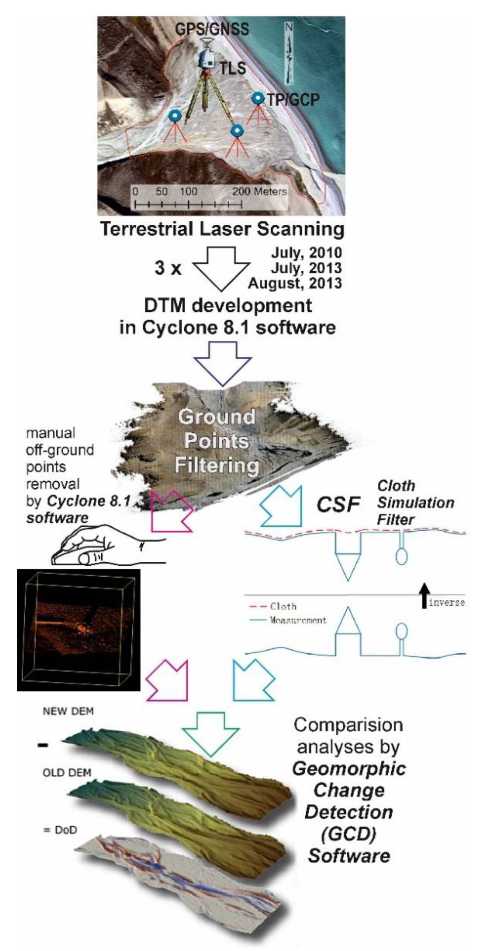
The measurement data from each campaign were integrated into the DTM by Leica’s Cyclone 8.1 software (Figure 2).
The point clouds in each of the three DTMs were then classified in order to separate the ground points. The classification was performed by adopting two methods; one done manually by the author and the other done automatically by using the CSF algorithm [28].
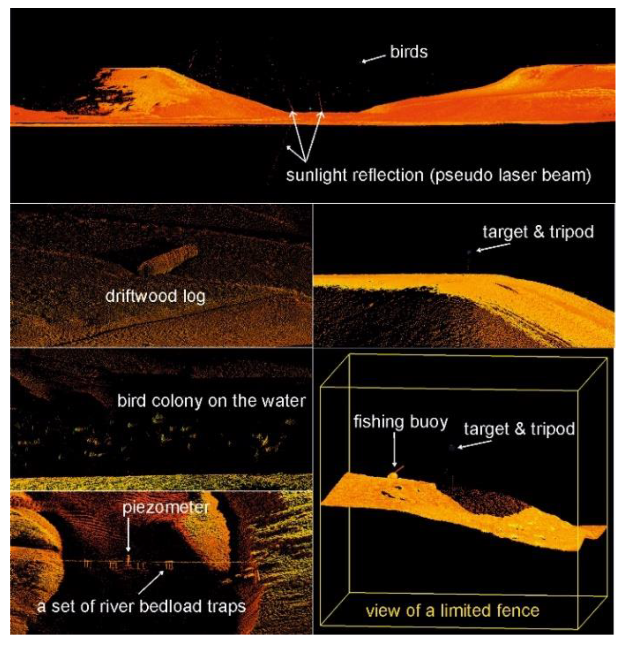
The ‘manual’ ground point classification was carried out in Leica Cyclone 8.1 software by removing all off-ground objects from the point cloud (Figure 2). As the High Arctic does not have any high vegetation (only dwarf vegetation and there is little of it in the valley floor), off-ground objects were limited to the following: living organisms (humans, birds, insects), objects abandoned in the coastal area during storms (fishing buoys, driftwood logs, fragments of a wooden winch), measurement installations (traps, piezometers, meteorological stations) and ‘noise’, i.e., points representing non-existent objects related to the misinterpretation of the sun’s rays directly striking the mirror of the scanner at an angle of about 45 degrees and the refraction of laser beams at the edge of water (Figure 3). The ‘limited fence’ function was used to remove off-ground points from the ‘view’ module, which made it possible to work on a fragment of the cloud that had been selected by the operator (Figure 3). This function significantly reduced the unintentional elimination of points from the cloud by the operator. At the same time, raw DTMs were filtered with the CSF algorithm (Figure 2) as a plug-in for CloudCompare 2.11. The following advanced parameter was used: the slope processing was set to ‘active’ (the valley section varies in altitude); then (1) the Cloth resolution was set to 0.1 m (the value refers to the grid size of cloth that was used to cover the terrain); (2) the max iterations were set to 1000 (the value refers to the maximum iteration counts of terrain simulation) and (3) the classification threshold was set to 0.1 m (the value of the threshold to classify the point clouds into ground as well as non-ground parts, which was based on the distances between points and the simulated terrain). In settings (1) and (3), respectively, the lower of the available units was used that was then the same as the unit in the point clouds processing. Lastly, using LP360 7.0 software, six ground point DTMs were converted into triangulated irregular network (TIN) models and further rasterized as a GeoTIFF with 0.1 m resolution to produce three pairs of DEMs (Figure 2).
2.2.3. Surface Change Detection by DEM of Difference (DoD)
For the purpose of obtaining information about the influence that the classification method has on the range of uncertainty in the estimation of surface and volume differences, three pairs of DEMs (prepared in exactly the same manner as mentioned above) were analyzed in Geomorphic Change Detection 7.4.4 (GCD) plug-in version for ArcGIS 10.8 software (Figure 2). According to the guidelines, as stated by the author of the DoD method [13], the approach, which is founded on the error assessment based on the spatial variable, was applied in order to calibrate the calculations.
There was an analysis done on data from the same source but differing in the method of separating the point clouds so the accuracy of the DEMs was closely related to the effectiveness of the ground point classification. The manually-classified DEM was assumed to be basal (new) and so least affected by classification errors. The DEM that resulted from Cloth Simulation Filtering was considered to be comparative (old) and more exposed to erroneous points, which had been omitted by the algorithm in Figure 2. Inherent to the calculation of the surface error for both DEMs was the assumption of the minimum detection level (minLoD) at ±0.1 m. A ‘mask’ for the AoI was applied, thus limiting the calculation results only to the gravel-cobbles surface of the 45,444 m2 alluvial fan. The final stage included applying ‘error propagation’ to determine the level of measurement uncertainty [15,33].
3. Results
The implementation of the various scanning methods in subsequent measurement campaigns as well as the application of two predefined measurement resolutions resulted in both the number of points and the average point density in the cloud being different. Both ‘manual’ and ‘automatic’ classification processes led to a reduction in the number of points within the range from 0.01% to 2.7% (Table 1). Out of the eleven individual point clouds from 2010, nine were made in high resolution. However, a relatively small number of scan stations produced a total of 52,358,443 points in the DTM, while the average density of points for the AoI equaled 345 pt/m2. Moreover, both of these parameters were similar to those effectively recorded in the third measurement campaign (August 2013) when the average resolution was predefined for all eleven scan stations. The result was a total number of 45,207,502 points in the DTM and an average point density of 309 pt/m2 for the AoI. The DTM from July 2013 was a fragment of the model of the whole valley so in addition to the eleven scan stations located at the bottom of the alluvial fan, the DTM supplemented points by taking them from seven other locations on the slopes as well as the lifted marine terraces plateau. Therefore, this last DTM was characterized by a much larger total number of points equal to 70,071,395 as well as a higher average point density for the AoI at 437 pt/m2 (Table 1).
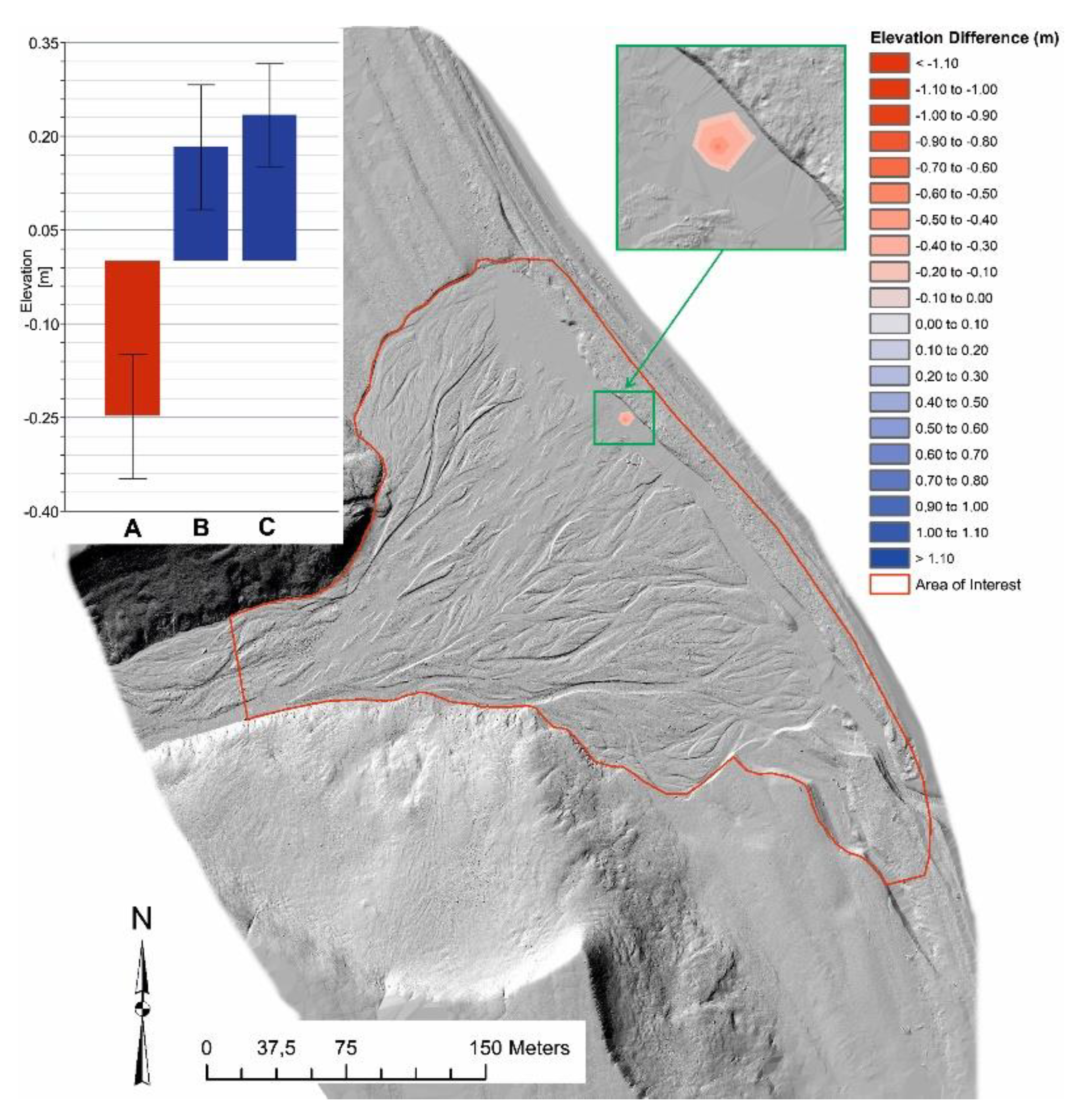
The analysis of surface differences carried out with the use of GCD software [12,14] made it possible to estimate the physical parameters of the gravel-cobble deposit, which was the result of errors in the CSF algorithm classification. The results of the DEMs comparison from 2010 show negligible differences between both methods of classifying the ground points (Figure 4; Table 2).
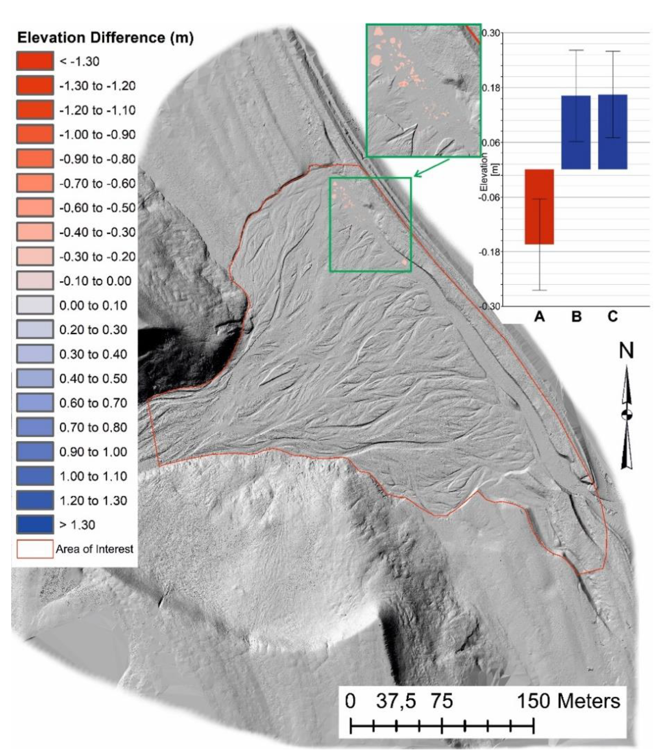
Surfaces that were misinterpreted by the CSF represented only 3% of the AoI. Insofar as lowered areas slightly predominated within the range of surfaces in the raw point cloud, the lowered areas at threshold values (minLoD = 0.1 m) constituted as much as 79% of them (Table 2). The height change diagram shows that the average total thickness of difference was 0.23 m (± 0.10) with an average net thickness difference of −0.16 m (± 0.08) (Figure 3). All error areas were concentrated in the north-east part of the AoI and occurred within or at the boundaries of water surfaces (Figure 4). The oval shape of these areas indicated that the CSF algorithm omitted small concentrated groups or even single points that were found below the water level.
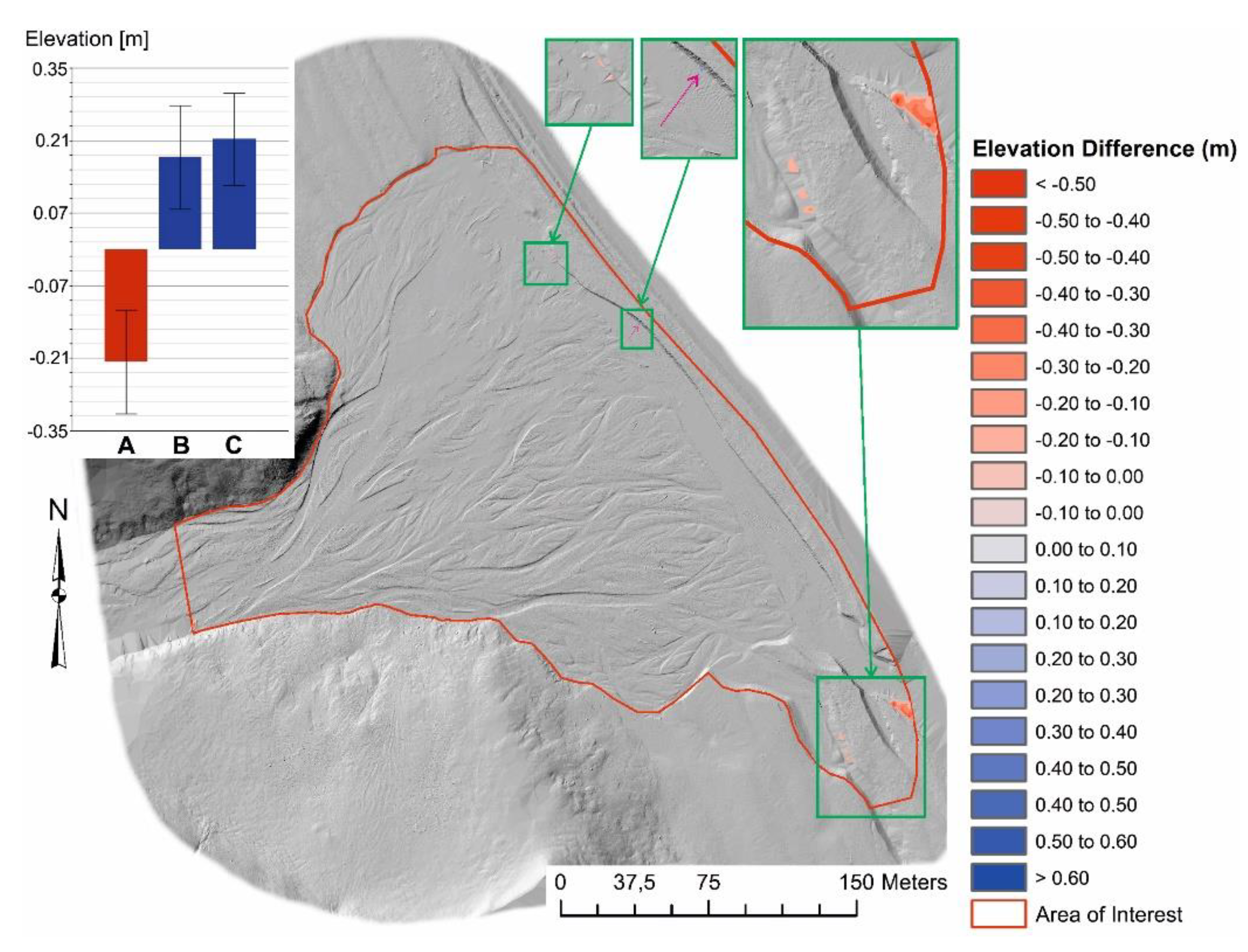
In relation to the data from July 2013, the area of detected changes was identical to the AoI area for raw point clouds whereas it was only 0.2% of the AoI area for the threshold values (minLoD = 0.1 m) (Table 3). Among the areas misinterpreted by the CSF, the raw PC was slightly dominated by elevated areas (52%) while for threshold values it was the lowered areas that prevailed (95%) (Table 3). An analysis of the height change diagram showed that the averages of the total as well as the net thickness of difference were smaller than in 2010 and were from 0.16 m (± 0.10) to −0.15 m (± 0.09), respectively (Figure 4). As in 2010, all of the error areas were concentrated in the north-east of the AoI where they occupied similar locations and took on comparable shapes (Figure 5).
In terms of the data from August 2013, the area of detected changes was less than 60% of the AoI area for raw point clouds whereas it was 0.1% of the AoI area for the threshold values (minLoD = 0.1 m), which was similar to the observations made in July (Table 4). Among the areas misinterpreted by the CSF, the raw PC was slightly dominated by elevated areas (52%) while for the threshold values, it was the lowered areas that prevailed (95%) (Table 4). An analysis of the height change diagram showed that the averages of the total and the net thickness of difference were similar to 2010 and were equal to 0.21 m (± 0.10) and −0.17 m (± 0.09), respectively (Figure 5). All of the error areas were concentrated on the right bank of the river in a section that was parallel to the storm dike. Lowered areas dominated there. Meanwhile, the largest area and height differences occurred coincidentally at the mouth of the river that flows into the fjord (Figure 6).
4. Discussion
In areas where mineral resources are extracted, the key issue is to quickly determine the quantities of extracted or exploitable mineral resources. An accurate estimation of deposit parameters requires taking into account three potential sources of uncertainty: (i) the physical properties of the material in the deposit, (ii) the measurement methodology along with the accuracy of the measuring equipment and also the measurement methods in the case of modern remote sensing (iii) the methods for classifying ground points as well as the interpolation of the ground surface and their respective analysis. In this context, a significant part of the research is focused on estimating the cubature or bulk density of the raw material under in situ conditions, all of the while using conventional and modern remote sensing methods such as digital close-range photogrammetry (structure from motion (SfM) photogrammetry) and terrestrial laser scanning. These works usually document relatively small (about 5%) differences between the parameters determined in a laboratory and those under field conditions by TLS [12]. This is all the more so because during the extraction or movement of the sediment resulting from natural processes (landslides, mud and rubble run-off, debris flow, etc.), the cohesion and loosening of the sediment structure is reduced. As a result, it is often found that the volume of the deposited material is larger than that of the erosion niche. Bremer and Sass [35] highlighted an average 7% prevalence of deposited volumes over the detected eroded volumes for two debris flow events in the Halltal (Austrian Alps). Kociuba [36] also pointed to a 6% growth of volume material that was deposited in a small alluvial fan that developed directly below a rill and suggested that this was due to the loosening of the transported material as well as multiple stages of aggradation (multilayer deposition on the cone). In fact, the loosening coefficient for the heterogeneous mineral resources of the perlite deposits was estimated to be 1.38 [12].
A similar uncertainty range (about 2%) is associated with the use of various algorithms for filtering ground points. Studies aimed at the accuracy of the algorithms most often focus on the following: comparing the effectiveness between the algorithms or deviations from differential morphological profiles and reference surfaces [37], discarding returns that exceed a threshold curvature calculated from a surface that is interpolated using a thin plated spline [38], identifying in the meantime the lowest elevation point in every cell that is defined by an operator and, finally, creating a surface by interpolating these lowest points [39].
The key classification problems are presented in many studies on the effectiveness of algorithms that classify ALS data; however, none of these works involve data obtained through terrestrial scanning [23,27,28,37,40,41]. Although some researchers think that the most effective classification of TLS point clouds is performed by manual point removal [42], others consider that automation of the classification process, especially with algorithms that do not use the altitude threshold parameter, significantly increases the time efficiency and eliminates errors resulting from operator bias [21].
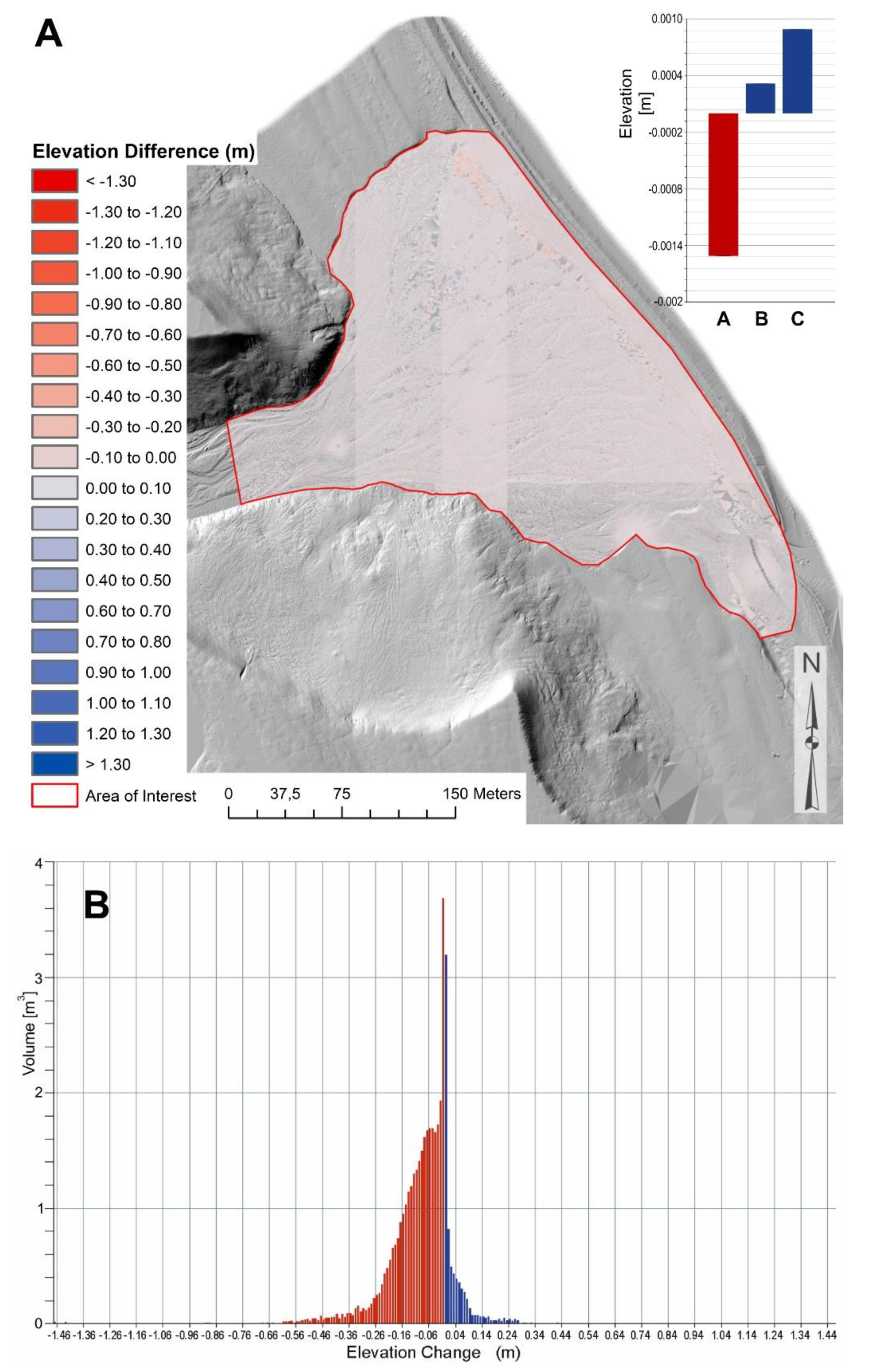
Many algorithms that successfully classify ground points from ALS data are much less effective in separating them from TLS clouds. This results, among others, from the following: (i) a different angle of attack of the laser beam, (ii) a significantly higher number of points in the cloud, (iii) a different density of points in the cloud (density decreases with the distance from the scanner) but also (iv) a lack of appropriate recommendations for the selection of classification parameters [24]. Available as a plug-in for Cloud Compare software, the CSF algorithm [28] is one of the few commonly available algorithms that has a graphical interface with tooltips or hints, which are shown in both graphic and text form, in order to help the user understand how the algorithm works and to significantly accelerate the definition of optimal parameters. It also provides relatively good results in the classification of ground points from TLS data due to its use of two factors; the inversion of the ground surface and coating the ground surface with a simulated cloth of specific strength and thickness [28]. This makes it possible to eliminate the previously mentioned differences between ALS and TLS clouds, which influence the less effective results of other algorithms that contain TLS data. Unfortunately, what is a ‘strength’ is also a minor ‘weakness’ of this method. The algorithm is sensitive to errors occurring on the boundary between land and water where we often have to deal with noise. As this study shows, it is below the water surface that the noise is not always filtered out by the CSF. Keeping these points leads to an artificial lowering of the surface. In addition, defining the thickness of the canvas results in the possibility of ‘shearing’ objects that exceed this parameter; for example, large boulders buried at the bottom of a gravel-cobble bed creek. The results of the study show that the applied method of filtering ground points by the CSF to a small extent increases the scope of uncertainty in estimating the quantitative parameters of the analyzed resource. The study adopted a range of MinLoD = 0.1 m as this value referred to the smallest possible key parameters defined in the CSF—the thickness and flexibility of the cloth. It also referred to the raster cell size used in this study. Working with this limitation caused the values that were estimated as the DoD threshold parameterizing the areas that deviated from the reference area to be only about 1% of the AoI area. The assumption of MinLoD = 0 as well as the application of error propagation made the values for raw data and the estimated DoD threshold area overlay in up to 100% of the AoI area. The obtained values for the raw and threshold data were also the same. However, the graphical representation of the DoD of these changes and the height indicators show (Figure 7A,B) that the uncertainty associated with the accuracy of the algorithm is not a parameter that significantly affects the results of the quantitative assessment of the deposit resources.
5. Conclusions
This paper answers the question as to what extent the method of classifying ground points affects the result of a mineral resource volume estimation. During the analysis of DTM pairs derived from the same area at three different times, it was shown that the errors associated with the applied automatic algorithm of ground points classification did not differ significantly from the model developed by the operator (manual noise removal). The main accomplishments of this research work are the two methods that were used in the classification of ground points (manual removal and CSF). These generated very similar results for cases of mineral resource exploitation (or potential exploitation) areas such as gravel, perlite and sand and in the analyses of changes to the land’s natural surface without vegetation cover such as landslides, river valleys, etc.
The CSF algorithm’s automatic classification errors minimally affected the scope of the quantitative estimation of the resource. In the assumed range of MinLoD = 0.1 m, the errors only pertained to about 1% of the AoI area while their average height deviation values were determined not to usually exceed 0.2 m.
The limitations of this study are that the analyses that were conducted in the course of the study have broadened the knowledge base in this topic area although it has only been in relation to a specific type of resource (gravel-cobble deposits) and two classification methods (manual and CSF).
In DoD analyses, any uncertainties that are associated with errors in the interpretation of the ground surface are usually not taken into account. We may question whether this is the right approach. It seems that due to the intensive development of current and newly available classification algorithms, this topic should be further explored and it ought to be looked at in terms of testing both new algorithms and other types of resources along with their conditions of occurrence.
Funding
This research received no external funding.
Acknowledgments
The field research with the application of TLS was conducted during the 22nd and 25th Polar Expedition of UMCS to Spitsbergen. The Measurement campaign 2013 was financed from the funds of the project of the National Science Centre 2011/01/B/ST10/06996 ‘Mechanisms of fluvial transport and sediment supply to channels of Arctic rivers with various hydrological regimes (SW Spitsbergen)’. I would like to thank all of participants of the expeditions for their assistance in conducting surveys and would particularly like to thank MSc. Eng. Waldemar Kubisz and the management of Leica Geosystems Polska for providing the measurement equipment in 2010 and active participation in both the research and development of the model. The author is grateful for the English language proofreading by Luke Boczkowski.
Conflicts of Interest
The author declares no conflict of interest.
References
- Yan, W.Y.; Shaker, A.; El-Ashmawy, N. Urban land cover classification using airborne LiDAR data: A review. Remote Sens. Environ. 2015, 158, 295–310. [Google Scholar] [CrossRef]
- Kociuba, W. Analysis of geomorphic changes and quantification of sediment budgets of a small Arctic valley with the application of repeat TLS surveys. Z. Geomorphol. 2017, 61, 105–120. [Google Scholar] [CrossRef]
- Milan, D.J.; Heritage, G.L.; Hetherington, D. Application of a 3D laser scanner in the assessment of erosion and deposition volumes and channel change in a proglacial river. Earth Surf. Process. Landf. 2007, 32, 1657–1674. [Google Scholar] [CrossRef]
- Bangen, S.G.; Wheaton, J.M.; Bouwes, N.; Bouwes, B.; Jordan, C. A methodological intercomparison of topographic survey techniques for characterizing wadeable streams and rivers. Geomorphology 2014, 206, 343–361. [Google Scholar] [CrossRef]
- Wack, R.; Wimmer, A. Digital Terrain Models from Airborne Laser Scanner Data—A Grid Based Approach; International Archives of Photogrammetry and Remote Sensing: Graz, Austria, 2002; Volume 34. [Google Scholar]
- Wężyk, P.; Szostak, M.; Krzaklewski, W.; Pająk, M.; Pierzchalski, M.; Szwed, P.; Hawryło, P.P.; Ratajczak, M. Landscape monitoring of post-industrial areas using LiDAR and GIS technology. Geod. Cartogr. 2015, 64, 125–137. [Google Scholar] [CrossRef] [Green Version]
- Boyko, A.; Funkhouser, T. Extracting roads from dense point clouds in large scale urban environment. ISPRS J. Photogramm. Remote Sens. 2011, 66, S2–S12. [Google Scholar] [CrossRef] [Green Version]
- Wang, J.; González-Jorge, H.; Lindenbergh, R.; Arias-Sánchez, P.; Menenti, M. Automatic estimation of excavation volume from laser mobile mapping data for mountain road widening. Remote Sens. 2013, 5, 4629–4651. [Google Scholar] [CrossRef] [Green Version]
- Quackenbush, L.J.; Im, I.; Zuo, Y. Road extraction: A review of LiDAR-focused studies. Remote Sens. Nat. Resour. 2013, 7, 155–169. [Google Scholar]
- Jaboyedoff, M.; Oppikofer, T.; Abellan, A.; Derron, M.H.; Alexandre, L.; Metzger, R.; Pedrazzini, A. Use of LIDAR in landslide investigations: A review. Nat. Hazards 2015, 61, 5–28. [Google Scholar] [CrossRef] [Green Version]
- Teo, T.-A.; Wu, H.-M. Analysis of land cover classification using multi-wavelength LiDAR system. Appl. Sci. 2017, 7, 663. [Google Scholar] [CrossRef] [Green Version]
- Blistan, P.; Jacko, S.; Kovanič, Ľ.; Kondela, J.; Pukanská, K.; Bartoš, K. TLS and SfM approach for bulk density determination of excavated heterogeneous raw materials. Minerals 2020, 10, 174. [Google Scholar] [CrossRef] [Green Version]
- Wheaton, J.M. Uncertainty in Morphological Sediment Budgeting of Rivers. Ph.D. Thesis, University of Southampton, Southampton, UK, 2008. [Google Scholar]
- Heritage, G.L.; Milan, D.J.; Large, A.R.G.; Fuller, I.C. Influence of survey strategy and interpolation model on DEM quality. Geomorphology 2009, 112, 334–344. [Google Scholar] [CrossRef]
- Wheaton, J.M.; Brasington, J.; Darby, S.E.; Sear, D.A. Accounting for uncertainty in DEMs from repeat topographic surveys: Improved sediment budgets. Earth Surf. Process. Landf. 2010, 35, 136–156. [Google Scholar] [CrossRef]
- Wheaton, J.M.; Brasington, J.; Darby, S.E.; Sear, D.A.; Kasprak, A. Morphodynamic signatures of braiding mechanisms as expressed through change in sediment storage in a gravel-bed river. J. Geophys. Res. Earth Surf. 2013, 118, 759–779. [Google Scholar] [CrossRef] [Green Version]
- Milan, D.J.; Heritage, G.L.; Large, A.R.G.; Fuller, I.C. Filtering spatial error from DEMs: Implications for morphological change estimation. Geomorphology 2011, 125, 160–171. [Google Scholar] [CrossRef]
- Schwendel, A.C.; Fuller, I.C.; Death, R.G. Assessing DEM interpolation methods for effective representation of upland stream morphology for rapid appraisal of bed stability. River Res. Appl. 2012, 28, 567–584. [Google Scholar] [CrossRef] [Green Version]
- Axelsson, P. DEM generation from laser scanner data using adaptive TIN models. Int. Arch. Photogramm. Remote Sens. 2000, 33, 203–210. [Google Scholar]
- ASPRS Standard LIDAR Point Classes 2008. Available online: https://www.asprs.org/a/society/committees/standards/asprs_las_format_v12.pdf (accessed on 15 May 2020).
- Chen, Z.; Gao, B.; Devereux, B. State-of-the-art: DTM generation using airborne LIDAR data. Sensors 2017, 17, 150. [Google Scholar] [CrossRef] [Green Version]
- Chen, C.; Yue, T. A method of DEM construction and related error analysis. Comput. Geosci. 2010, 36, 717–725. [Google Scholar] [CrossRef]
- Sithole, G.; Vosselman, G. Report: ISPRS Comparison of Filters; Department of Geodesy, Faculty of Civil Engineering and Geosciences, Delft University of Technology: Delft, The Netherlands, 2003. [Google Scholar]
- Montealegre, A.L.; Lamelas, M.T.; de la Riva, J. A comparison of open-source LiDAR filtering algorithms in a Mediterranean forest environment. IEEE J. Sel. Top. Appl. Earth Obs. Remote Sens. 2015, 8, 4072–4085. [Google Scholar] [CrossRef] [Green Version]
- Kraus, K.; Pfeifer, N. Determination of terrain models in wooded areas with airborne laser scanner data. ISPRS J. Photogramm. Remote Sens. 1998, 53, 193–203. [Google Scholar] [CrossRef]
- Pingel, T.J.; Clarke, K.C.; McBride, W.A. An improved simple morphological filter for the terrain classification of airborne LIDAR data. ISPRS J. Photogramm. Remote Sens. 2013, 77, 21–30. [Google Scholar] [CrossRef]
- Meng, X.; Currit, N.; Zhao, K. Ground filtering algorithms for airborne LiDAR data: A review of critical issues. Remote Sens. 2010, 2, 833–860. [Google Scholar] [CrossRef] [Green Version]
- Zhang, W.; Qi, J.; Wan, P.; Wang, H.; Xie, D.; Wang, X.; Yan, G. An easy-to-use airborne LiDAR data filtering method based on cloth simulation. Remote Sens. 2016, 8, 501. [Google Scholar] [CrossRef]
- Cereda, S. A comparison of Different Neural Networks for Agricultural Image Segmentation. Master’s Thesis, Politecnico di Milano, Milano, Italy, 2017. [Google Scholar]
- Dyson, J.; Mancini, A.; Frontoni, E.; Zingaretti, P. Deep learning for soil and crop segmentation from remotely sensed data. Remote Sens. 2019, 11, 1859. [Google Scholar] [CrossRef] [Green Version]
- Kociuba, W.; Krząstek, P.; Superson, J. Combining GPS-RTK and rephotographic methodologies for the assessment of transformations of the ephemeral landforms of the near foreland of a valley glacier (Scottbreen, Svalbard). Z. Geomorphol. 2016, 60, 29–44. [Google Scholar] [CrossRef]
- Harasimiuk, M.; Gajek, G. Tectonic and lithology. In Geographical Environment of NW Part of Wedel Jarlsberg Land (Spitsbergen, Svalbard); Zagórski, P., Harasimiuk, M., Rodzik, J., Eds.; Wydawnictwo UMCS: Lublin, Poland, 2013; pp. 34–47. [Google Scholar]
- Leica-Geosystems. Leica ScanStation C10-Datasheet. 2012. Available online: http://www.leica-geosystems.co.uk/downloads123/hds/hds/ScanStation%20C10/brochures-datasheet/Leica_ScanStation_C10_DS_en.pdf (accessed on 15 May 2020).
- Kociuba, W. Assessment of sediment sources throughout the proglacial area of a small Arctic catchment based on high-resolution digital elevation models. Geomorphology 2017, 287, 73–89. [Google Scholar] [CrossRef]
- Bremer, M.; Sass, O. Combining airborne and terrestrial laser scanning for quantifying erosion and deposition by a debris flow event. Geomorphology 2012, 138, 49–60. [Google Scholar] [CrossRef]
- Kociuba, W.; Kubisz, W.; Zagórski, P. Use of terrestrial laser scanning (TLS) for monitoring and modelling of geomorphic processes and phenomena at a small and medium spatial scale in Polar environment (Scott River—Spitsbergen). Geomorphology 2014, 212, 84–96. [Google Scholar] [CrossRef]
- Žalik, B.; Mongus, D.; Lukač, N. Ground and building extraction from LiDAR data based on differential morphological profiles and locally fitted surfaces. ISPRS J. Photogramm. Remote Sens. 2014, 93, 145–156. [Google Scholar]
- Evans, J.S.; Hudak, A.T. A multiscale curvature algorithm for classifying discrete return lidar in forested environments. IEEE Trans. Geosci. Remote Sens. 2007, 45, 1029–1038. [Google Scholar] [CrossRef]
- Streutker, D.; Glenn, N. LiDAR measurement of sagebrush steppe vegetation heights. Remote Sens. Environ. 2006, 102, 135–145. [Google Scholar] [CrossRef]
- Tinkham, W.T.; Hongyu, H.; Smith, A.M.S.; Shrestha, R.; Falkowski, M.J.; Hudak, A.T.; Link, T.E.; Glenn, N.F.; Marks, D.G. A comparison of two open source LiDAR surface classification algorithms. Remote Sens. 2011, 3, 638–649. [Google Scholar] [CrossRef] [Green Version]
- Mongus, D.; Zalik, B. Parameter-free ground filtering of LiDAR data for automatic DTM generation. ISPRS J. Photogramm. Remote Sens. 2012, 67, 1–12. [Google Scholar] [CrossRef]
- Kociuba, W.; Janicki, G.; Rodzik, J.; Stępniewski, K. Comparison of volumetric and remote sensing methods (TLS) for assessing the development of a permanent forested loess gully. Nat. Hazards 2015, 79, 139–158. [Google Scholar] [CrossRef]
Figure 1.
(A) Location of the study area. The mouth section of the gravel-cobble Scott River valley floor (north-west part of the Wedel Jarlsberg Land, south-west Svalbard). Red line: area of interest (AoI). Source of satellite image in the background: Image Landsat/Copernicus, Image IBACO; ESRI, DigitalGlobe, GeoEye, Earthstar Geographics, CNES/Airbus DS, USDA, USGS, AeroGRID, IGN and the GIS User Community. (B) The elevation of the Area of Interest: A–B longitudinal profile; C–D cross-profile.

Figure 2.
Framework of research method. Sources: Cloth Simulation Filter (CSF) diagram [28], Geomorphic Change Detection (GCD) diagram http://gcd.riverscapes.xyz, [13,15].
Figure 2.
Framework of research method. Sources: Cloth Simulation Filter (CSF) diagram [28], Geomorphic Change Detection (GCD) diagram http://gcd.riverscapes.xyz, [13,15].

Figure 3.
A few object types of the off-ground points in the raw point cloud.

Figure 4.
Digital elevation model (DEM) of difference (DoD) for the AoI (July 2010 with MinLoD = 0.1). Hillshade map is shown behind the DoD for context. Description of the bars in the diagram: (A) Average Depth of Lowering; (B) Average Depth of Raising; (C) Average Total Thickness Difference.
Figure 4.
Digital elevation model (DEM) of difference (DoD) for the AoI (July 2010 with MinLoD = 0.1). Hillshade map is shown behind the DoD for context. Description of the bars in the diagram: (A) Average Depth of Lowering; (B) Average Depth of Raising; (C) Average Total Thickness Difference.

Figure 5.
DEM of difference (DoD) for the AoI (July 2013 with MinLoD = 0.1). Hillshade map is shown behind the DoD for context. Description of the bars in the diagram: (A) Average Depth of Lowering; (B) Average Depth of Raising; (C) Average Total Thickness Difference.
Figure 5.
DEM of difference (DoD) for the AoI (July 2013 with MinLoD = 0.1). Hillshade map is shown behind the DoD for context. Description of the bars in the diagram: (A) Average Depth of Lowering; (B) Average Depth of Raising; (C) Average Total Thickness Difference.

Figure 6.
DEM of difference (DoD) for the AoI (August 2013 with MinLoD = 0.1). Hillshade map is shown behind the DoD for context. Description of the bars in the diagram: (A) Average Depth of Lowering; (B) Average Depth of Raising; (C) Average Total Thickness Difference.
Figure 6.
DEM of difference (DoD) for the AoI (August 2013 with MinLoD = 0.1). Hillshade map is shown behind the DoD for context. Description of the bars in the diagram: (A) Average Depth of Lowering; (B) Average Depth of Raising; (C) Average Total Thickness Difference.

Figure 7.
(A) DEM of difference (DoD) for the AoI (July 2013 with MinLoD = 0). Hillshade map is shown behind the DoD for context. (B) Histograms of volume and area changes of AoI. Description of the bars in the diagram: (A) Average Depth of Lowering; (B) Average Depth of Raising; (C) Average Total Thickness Difference.


Table 1.
Digital Terrain Model (DTM) model parameters from the three measurement campaigns.
| Parameter | Unit | July 2010 | July 2013 | August 2013 |
|---|---|---|---|---|
| Total number of points (raw DTM) | pt | 52,358,443 | 70,071,395 | 45,207,502 |
| Point density at Area of Interest (AoI) | pt/m2 | 345 | 437 | 309 |
| Total number of ground points (manually removed) | pt | 52,351,107 | 68,389,716 | 45,121,473 |
| Total number of ground points (CSF filtered) | pt | 52,121,610 | 68,187,224 | 45,046,205 |
| Percent of changes (manually removed DTM) | % | 0.01 | 2.40 | 0.19 |
| Percent of changes (CSF filtered DTM) | % | 0.45 | 2.69 | 0.36 |
Table 2.
Changes in physical parameters of the Area of Interest in July 2010 calculated volumetrically with reference to the total volume of the gravel-cobble material’s net change recorded by the DoD (both lowering and raising) from the manually cleaned-up (new) to the CSF-filtered (old) DTM. The uncertainty analysis was calculated by simply using the minimum level of detection (minLoD) approach while accounting for a uniform error of 0.1 m.
| Attribute | Raw | Thresholded DoD Estimate: | ||
|---|---|---|---|---|
| Areal Metrics | % of AoI | |||
| Total Area of Surface Lowering (m²) | 724 | 48 | 1.6% | |
| Total Area of Surface Raising (m²) | 716 | 13 | 1.6% | |
| Total Area of Detectable Change (m²) | 1440 | 61 | 4.0% | |
| Total Area of Interest (m²) | 45,444 | NA | NA | |
| Total Volumetric Metrics | ±Error Volume | % Error | ||
| Total Volume of Surface Lowering (m³) | 21 | 12 | ±5 | 40% |
| Total Volume of Surface Raising (m³) | 9 | 2 | ±1 | 55% |
| Total Volume of Difference (m³) | 30 | 14 | ±6 | 43% |
| Total Net Volume Difference (m³) | −12 | −10 | ±5 | −52% |
| Vertical Averages: | ||||
| Average Depth of Surface Lowering (m) | 0.03 | 0.25 | ±0.100 | 40% |
| Average Depth of Surface Raising (m) | 0.01 | 0.18 | ±0.100 | 55% |
| Average Total Thickness of Difference (m) for Area of Interest | 0.02 | 0.01 | ±0.004 | 43% |
| Average Net Thickness Difference (m) for Area of Interest | −0.01 | −0.01 | ±0.003 | −52% |
| Percentages (by volume) | ||||
| Percent Elevation Lowering | 69% | 84% | ||
| Percent Surface Raising | 31% | 16% | ||
| Percent Imbalance (departure from equilibrium) | −19% | −34% | ||
| Net to Total Volume Ratio | −38% | −67% | ||
NA = not available.
Table 3.
Changes in physical parameters of the Area of Interest in July 2013 calculated volumetrically with reference to the total volume of the gravel-cobble material’s net change recorded by the DoD (both lowering and raising) from the manually cleaned-up (new) to the CSF-filtered (old) DTM. The uncertainty analysis was calculated by simply using the minimum level of detection (minLoD) approach while accounting for a uniform error of 0.1 m.
| Attribute | Raw | Thresholded DoD Estimate: | ||
|---|---|---|---|---|
| Areal Metrics | % of AoI | |||
| Total Area of Surface Lowering (m²) | 21,977 | 89 | 0.40% | |
| Total Area of Surface Raising (m²) | 23,467 | 5 | 0.02% | |
| Total Area of Detectable Change (m²) | 45,444 | 94 | 0.21% | |
| Total Area of Interest (m²) | 45,444 | NA | NA | |
| Total Volumetric Metrics | ±Error Volume | % Error | ||
| Total Volume of Surface Lowering (m³) | 33 | 15 | ± 9 | 61% |
| Total Volume of Surface Raising (m³) | 7 | 1 | ± 1 | 62% |
| Total Volume of Difference (m³) | 41 | 15 | ± 9 | 61% |
| Total Net Volume Difference (m³) | −26 | −14 | ± 9 | −65% |
| Vertical Averages: | ||||
| Average Depth of Surface Lowering (m) | 0.0015 | 0.1645 | ± 0.1000 | 61% |
| Average Depth of Surface Raising (m) | 0.0003 | 0.1619 | ± 0.1000 | 62% |
| Average Total Thickness of Difference (m) for Area of Interest | 0.0009 | 0.0003 | ± 0.0002 | 61% |
| Average Net Thickness Difference (m) for Area of Interest | −0.0006 | −0.0003 | ± 0.0002 | −65% |
| Percentages (by volume) | ||||
| Percent Elevation Lowering | 82% | 95% | ||
| Percent Surface Raising | 18% | 5% | ||
| Percent Imbalance (departure from equilibrium) | −32% | −45% | ||
| Net to Total Volume Ratio | −63% | −89% | ||
NA = not available.
Table 4.
Changes in physical parameters of the Area of Interest in July 2013 calculated volumetrically with reference to the total volume of the gravel-cobble material’s net change recorded by the DoD (both lowering and raising) from the manually cleaned-up (new) to the CSF-filtered (old) DTM. The uncertainty analysis was calculated by simply using the minimum level of detection (minLoD) approach while accounting for a uniform error of 0.1 m.
| Attribute | Raw | Thresholded DoD Estimate: | ||
|---|---|---|---|---|
| Areal Metrics | % of AoI | |||
| Total Area of Surface Lowering (m²) | 13,595 | 91 | 0.67% | |
| Total Area of Surface Raising (m²) | 13,376 | 13 | 0.10% | |
| Total Area of Detectable Change (m²) | 26,971 | 104 | 0.39% | |
| Total Area of Interest (m²) | 45,444 | NA | NA | |
| Total Volumetric Metrics | ±Error Volume | % Error | ||
| Total Volume of Surface Lowering (m³) | 32 | 20 | ± 9 | 46% |
| Total Volume of Surface Raising (m³) | 11 | 2 | ± 1 | 56% |
| Total Volume of Difference (m³) | 43 | 22 | ± 10 | 47% |
| Total Net Volume Difference (m³) | −21 | −18 | ± 9 | −52% |
| Vertical Averages: | ||||
| Average Depth of Surface Lowering (m) | 0.002 | 0.217 | 0.1000 | 46% |
| Average Depth of Surface Raising (m) | 0.001 | 0.178 | 0.1000 | 56% |
| Average Total Thickness of Difference (m) for Area of Interest | 0.002 | 0.001 | 0.0004 | 47% |
| Average Net Thickness Difference (m) for Area of Interest | −0.001 | −0.001 | 0.0003 | −52% |
| Percentages (by volume) | ||||
| Percent Elevation Lowering | 75% | 90% | ||
| Percent Surface Raising | 25% | 10% | ||
| Percent Imbalance (departure from equilibrium) | −25% | −40% | ||
| Net to Total Volume Ratio | −49% | −80% | ||
NA = not available.
Publisher’s Note: MDPI stays neutral with regard to jurisdictional claims in published maps and institutional affiliations. |
© 2020 by the author. Licensee MDPI, Basel, Switzerland. This article is an open access article distributed under the terms and conditions of the Creative Commons Attribution (CC BY) license (http://creativecommons.org/licenses/by/4.0/).
Share and Cite
MDPI and ACS Style
Kociuba, W. Different Paths for Developing Terrestrial LiDAR Data for Comparative Analyses of Topographic Surface Changes. Appl. Sci. 2020, 10, 7409. https://0-doi-org.brum.beds.ac.uk/10.3390/app10217409
AMA Style
Kociuba W. Different Paths for Developing Terrestrial LiDAR Data for Comparative Analyses of Topographic Surface Changes. Applied Sciences. 2020; 10(21):7409. https://0-doi-org.brum.beds.ac.uk/10.3390/app10217409
Chicago/Turabian StyleKociuba, Waldemar. 2020. "Different Paths for Developing Terrestrial LiDAR Data for Comparative Analyses of Topographic Surface Changes" Applied Sciences 10, no. 21: 7409. https://0-doi-org.brum.beds.ac.uk/10.3390/app10217409
Note that from the first issue of 2016, this journal uses article numbers instead of page numbers. See further details here.