A New “Good and Bad Groups-Based Optimizer” for Solving Various Optimization Problems

Abstract

Optimization is the science that presents a solution among the available solutions considering an optimization problem’s limitations. Optimization algorithms have been introduced as efficient tools for solving optimization problems. These algorithms are designed based on various natural phenomena, behavior, the lifestyle of living beings, physical laws, rules of games, etc. In this paper, a new optimization algorithm called the good and bad groups-based optimizer (GBGBO) is introduced to solve various optimization problems. In GBGBO, population members update under the influence of two groups named the good group and the bad group. The good group consists of a certain number of the population members with better fitness function than other members and the bad group consists of a number of the population members with worse fitness function than other members of the population. GBGBO is mathematically modeled and its performance in solving optimization problems was tested on a set of twenty-three different objective functions. In addition, for further analysis, the results obtained from the proposed algorithm were compared with eight optimization algorithms: genetic algorithm (GA), particle swarm optimization (PSO), gravitational search algorithm (GSA), teaching–learning-based optimization (TLBO), gray wolf optimizer (GWO), and the whale optimization algorithm (WOA), tunicate swarm algorithm (TSA), and marine predators algorithm (MPA). The results show that the proposed GBGBO algorithm has a good ability to solve various optimization problems and is more competitive than other similar algorithms.

1. Introduction

Optimization is the process in which the best solution (based on a set of constraints) to a particular problem is selected from a set of possible solutions. When an optimization problem is expressed, it must be modeled mathematically. In this modeling, the objectives of the problem and the limitations must be considered. In fact, an optimization problem has three main parts: the problem variables, the primary objects of the problem including constraints, and the secondary objects of the problem including the objective functions of the problem [1]. After designing the optimization problem, the next step is to solve the optimization problem using a suitable method. Optimization algorithms always have a special application in solving optimization problems. Optimization algorithms attempt to provide a solution by randomly scanning the search space.

An optimization problem has a definite optimal solution called global optimal. Optimization algorithms with random displacement in the problem search space provide a solution to a problem that is not necessarily global optimal, but close to it. For this reason, the solution obtained using optimization algorithms is called the quasi-optimal solution [2]. An optimization algorithm that presents a quasi-optimal solution closer to the global optimal solution is a more appropriate algorithm. This issue has led to the introduction of many optimization algorithms by researchers.

Various ideas have been applied in the design of optimization algorithms. These ideas are based on various natural phenomena, the behavior of living things, plants, the laws of physics, the rules of the game, etc. Optimization algorithms can be divided into four general groups based on the main design idea. These groups are physic-based optimization algorithms, swarm-based optimization algorithms, game-based optimization algorithms, and evolutionary-based optimization algorithms.

Physic-based optimization algorithms are designed based on simulations of processes and physical laws. Simulated annealing (SA) is a physics-based optimization algorithm modeled on the process of annealing metals [3]. In physics, annealing is the heat treatment during which changes the physical and sometimes chemical properties of a material occur. During this process, the metal is first heated, then kept at a certain temperature, and finally gradually cooled. The momentum search algorithm (MSA) is another physics-based optimization algorithm based on simulation of momentum laws and Newton’s laws of motion [4]. In MSA, the momentum that enters a bullet causes the bullet to motion toward quasi-optimal points in the search space. The gravitational search algorithm (GSA) is inspired by the physical law of gravity between objects at different distances from each other. According to this law, particles (or objects) in this universe always exert a force called gravity on each other, which is directly proportional to the mass of two objects and inversely proportional to the square of the distance between them. In GSA, the simulation of this concept is used in designing an optimizer for optimization problems [5].

Swarm-based optimization algorithms are modeled on various natural phenomena, the behavior of animals, plants, and other living organisms. Particle swarm optimization (PSO) is one of the oldest and most famous swarm-based optimization algorithms which is designed based on the simulation of group motion of birds [6]. The seagull optimization algorithm (SOA) is another swarm-based optimization algorithm that is designed based on simulating the migration and aggressive behavior of a seagull in nature [7]. The teaching–learning-based optimization (TLBO) was designed based on simulating the educational relationship between students and teacher that leads to student learning and progress. The TLBO has a mathematical model for teaching and learning, which is implemented in two stages teaching and learning [8]. The whale optimization algorithm (WOA) was developed based on simulation the social behavior of humpback whales in bubble-net hunting strategy [9]. The gray wolf optimizer (GWO) was inspired by the leadership hierarchy and hunting mechanism of gray wolves in nature. This natural behavior of gray wolves is such that four types of gray wolves such as alpha, beta, delta, and omega are used to simulate the leadership hierarchy. In addition, the three main steps of hunting— searching for prey, encircling prey, and attacking prey—are simulated in the GWO [10]. The tunicate swarm algorithm (TSA) was designed based on the simulation of jet propulsion and swarm behaviors of tunicates during the navigation and foraging process [11]. The marine predators algorithm (MPA) was inspired by the movement strategies that marine predators use when trapping their prey in the oceans. The main inspiration of the MPA is the widespread foraging strategy namely Lévy and Brownian movements in ocean predators along with optimal encounter rate policy in biological interaction between predator and prey [12].

Game-based optimization algorithms are designed using the potentials of various individual and group games. The orientation search algorithm (OSA) was designed by modeling the behavior of players and referees in the orientation game. In the orientation game, players move in the game space according to the direction specified by the reference [13]. The darts game optimizer (DGO) is another game-based optimization algorithm that was designed based on simulation of rules of the game and the behavior of the players in the darts game [14].

Evolutionary-based optimization algorithms as a family of stochastic search methods are inspired by the natural process of evolution of species. The genetic algorithm (GA) is an evolutionary-based optimization algorithm that was inspired by genetics and Darwin’s theory of evolution and is based on the survival of the fittest or natural selection. The GA simulates the reproductive process using three operators: selection, crossover, and mutation [15].

Although many optimization algorithms have been developed by scientists, no optimization algorithm can definitively provide global optimal solutions to the optimization problems. An optimization algorithm which provides the best solution for one optimization problem may fail to optimize another problem. The contribution of the authors and the main purpose of this paper was to design an optimization algorithm that could be used to solve optimization problems in various sciences. In designing the proposed algorithm, it was assumed that by increasing the power of exploration and exploitation of the algorithm, suitable quasi-optimal solutions are provided that are closer to the global optimal.

In this study, a new population-based optimization algorithm called the good and bad groups-based optimizer (GBGBO) was developed. The main idea of the proposed algorithm was to use more information from different population members in updating the whole population in such a way that instead of a good member, a good group, and instead of a bad member, a bad group would lead the population members. Thus, in each iteration, the status of the population members was updated based on two groups: The good group with the best values of the objective function and the bad group with the worst values of the objective function.

The rest of the article is organized in such a way that in Section 2, the proposed algorithm is introduced and modeled mathematically. In Section 3, the implementation of the proposed algorithm in the optimization is simulated. The Friedman rank test analysis is presented in Section 4. The analysis of the results and performance of the optimization algorithm is presented in Section 5. Section 6 provides conclusions and suggestions for future studies.

2. Good and Bad Groups-Based Optimizer

In this section, firstly the GBGBO is described, and then the mathematical modeling of the proposed algorithm is presented in order to implement in solving optimization problems.

The GBGBO is a population-based optimization algorithm, which is based on random scanning of the problem search space. The member of the population that has a better objective function as the best member of the population can direct the population of the algorithm to the optimal regions. However, the best member of the population may not provide the suitable amount for some problem variables. Thus, instead of just the best member of the population, GBGBO proposes a group of the best members to guide the population in the search space. This is also debatable for the worst member of the population. Instead of moving away from just the worst member of the population, GBGBO suggests moving away from a group of worst members. Thus, in GBGBO, population members update under the influence of two groups named the good group and the bad group. A good group consists of a certain number of the population members with better fitness function than other members and a bad group consists of a number of the population members with a worse fitness function than other members of the population.

The population of the GBGBO was defined using a matrix in which each row represented a member that proposed a solution to the optimization problem. The population matrix was first generated randomly and then updated according to the algorithm steps. This population matrix was specified in Equation (1).

$$X={\left[\begin{array}{c}\begin{array}{c}{X}_1\\ ⋮\\ X_i\end{array}\\ ⋮\\ X_N\end{array} |\begin{array}{ccccc}{x}_{1,1}& \cdots & x_{1,d}& \cdots & x_{1,m}\\ ⋮& \ddots & ⋮& ⋰& ⋮\\ x_{i,1}& \cdots & x_{i,d}& \cdots & x_{i,m}\\ ⋮& ⋰& ⋮& \ddots & ⋮\\ x_{N,1}& \cdots & x_{N,d}& \cdots & x_{N,m}\end{array}\right]}_{N\times m}$$

(1)

Here, $X$ is the population matrix, $X_i$ is the i-th population member, $x_{i,d}$ is the d-th dimension of the i-th population member, N is the number of population members, and m is the number of variables of the optimization problem. After determining the population matrix, the objective function of the optimization problem was evaluated based on each member of the population that represents a solution. The vector values of the fitness function are specified in Equation (2).

$$F={\left[\begin{array}{c}\begin{array}{c}{F}_1\\ ⋮\\ F_i\end{array}\\ ⋮\\ F_N\end{array} |\begin{array}{c}\begin{array}{c}F\left(X_1\right)\\ ⋮\\ F\left(X_i\right)\end{array}\\ ⋮\\ F\left(X_N\right)\end{array}\right]}_{N\times 1}$$

(2)

Here, $F$ is the fitness function value vector and $F_i$ is the fitness function value of the i-th population member.

Each optimization problem has a definite number of m variables that must be specified to optimize the objective function. In fact, the search space consists of m axes, each of which determines the value of a problem variable. In most optimization algorithms, a population member leads the population in the search space. That is, a good member leads the population in all axes. However, one or more other members may be more appropriate to guide the population in some axes. In addition, in some optimization algorithms, moving away from the worst population member is effective in updating and improving the population. The main idea of the GBGBO is to use the information of population members more effectively. Accordingly, instead of a good member leading the entire population in all axes, a group of good members was selected to lead the population. In addition, instead of just one bad member moving the algorithm away from the bad areas, a bad group was selected. In the GBGBO, the population members were updated based on two good and bad groups.

Good group updating:

The criterion for selecting good members was the value of the objective function. The number of NG members of the population that provide the best values of the objective function was selected as a good matrix.

Bad group updating:

As mentioned, the criterion for selecting bad members was also the value of the objective function. The number of NB members of the population that provided the worst values of the objective function was selected as the bad matrix.

In fact, if members of the population were arranged from the smallest to the largest value of the objective function, the NG number of the first member was selected as the good group and the NB number of the last member was selected as the bad group. Thus, based on the values of the fitness functions, the good group and the bad group could be calculated according to Equations (3) and (4).

$$GG={\left[\begin{array}{c}G{G}_1\\ ⋮\\ G{G}_i\\ ⋮\\ G{G}_N\end{array}|\begin{array}{ccccc}g{g}_{1,1}& \cdots & g{g}_{1,d}& \cdots & g{g}_{1,m}\\ ⋮& \ddots & ⋮& ⋰& ⋮\\ g{g}_{i,1}& \cdots & g{g}_{i,d}& \cdots & g{g}_{i,m}\\ ⋮& ⋰& ⋮& \ddots & ⋮\\ g{g}_{N_G,1}& \cdots & g{g}_{N_G,d}& \cdots & g{g}_{N_G,m}\end{array}\right]}_{N_G\times m}$$

(3)

$$BG={\left[\begin{array}{c}B{G}_1\\ ⋮\\ B{G}_i\\ ⋮\\ B{G}_N\end{array}|\begin{array}{ccccc}b{g}_{1,1}& \cdots & b{g}_{1,d}& \cdots & b{g}_{1,m}\\ ⋮& \ddots & ⋮& ⋰& ⋮\\ b{g}_{i,1}& \cdots & b{g}_{i,d}& \cdots & b{g}_{i,m}\\ ⋮& ⋰& ⋮& \ddots & ⋮\\ b{g}_{N_B,1}& \cdots & b{g}_{N_B,d}& \cdots & b{g}_{N_B,m}\end{array}\right]}_{N_B\times m}$$

(4)

Here, $GG$ is the good group, $G{G}_i$ is the i-th good member,$g{g}_{i,d}$ is the d-th dimension of the i-th good member, $N_G$ is the number of selected good members, $BG$ is the bad group, $B{G}_i$ is the i-th bad member,$b{g}_{i,d}$ is the d-th dimension of the i-th bad member, and $N_B$ is the number of selected bad members.

Each row of the population matrix as a population member was a proposed solution and indeed determined the variables of the problem. The best member of the population was the member that provided the best value for the objective function. Although the best member suggested appropriate values for the problem variables, it may not necessarily have been appropriate to guide the population in some variables. If the members of the algorithm population moved only under the guidance of the best member in the problem search space, all variables of each member moved towards the variables determined by the best member. In the GFBGO, a member of a good group was randomly selected to guide each variable of each member of the population. In fact, a good group member may have only led only a few variables of a population member in the search space, although a good group member may not have been selected to lead any variables. These concepts could also be developed for the worst members of the population and the bad group. This step of the GBGBO was simulated using Equations (5) and (6).

$$x_{i,d}=\{\begin{array}{l}{x}_{i,d}+rand\times \left(g{g}_{k,d}-2\times x_{i,d}\right), F_i<F_k^{GG}\\ x_{i,d}+rand\times \left(x_{i,d}-2\times g{g}_{k,d}\right), else\end{array} \& k\in 1:N_G$$

(5)

$$x_{i,d}=\{\begin{array}{l}{x}_{i,d}+rand\times \left(b{g}_{k,d}-2\times x_{i,d}\right), F_i<F_k^{BG}\\ x_{i,d}+rand\times \left(x_{i,d}-2\times b{g}_{k,d}\right), else\end{array} \& k\in 1:N_B$$

(6)

Here, $g{g}_{k,d}$ is the d-th dimension of selected good member to guide the d-th dimension of the ith population member, $F_k^{GG}$ is the objective function value of the k-th selected good member, $b{g}_{k,d}$ is the d-th dimension of selected bad member to guide the d-th dimension of the i-th population member, $F_k^{BG}$ is the objective function value of the k-th selected bad member, and rand is a random number with a normal distribution within the range from 0 to 1.

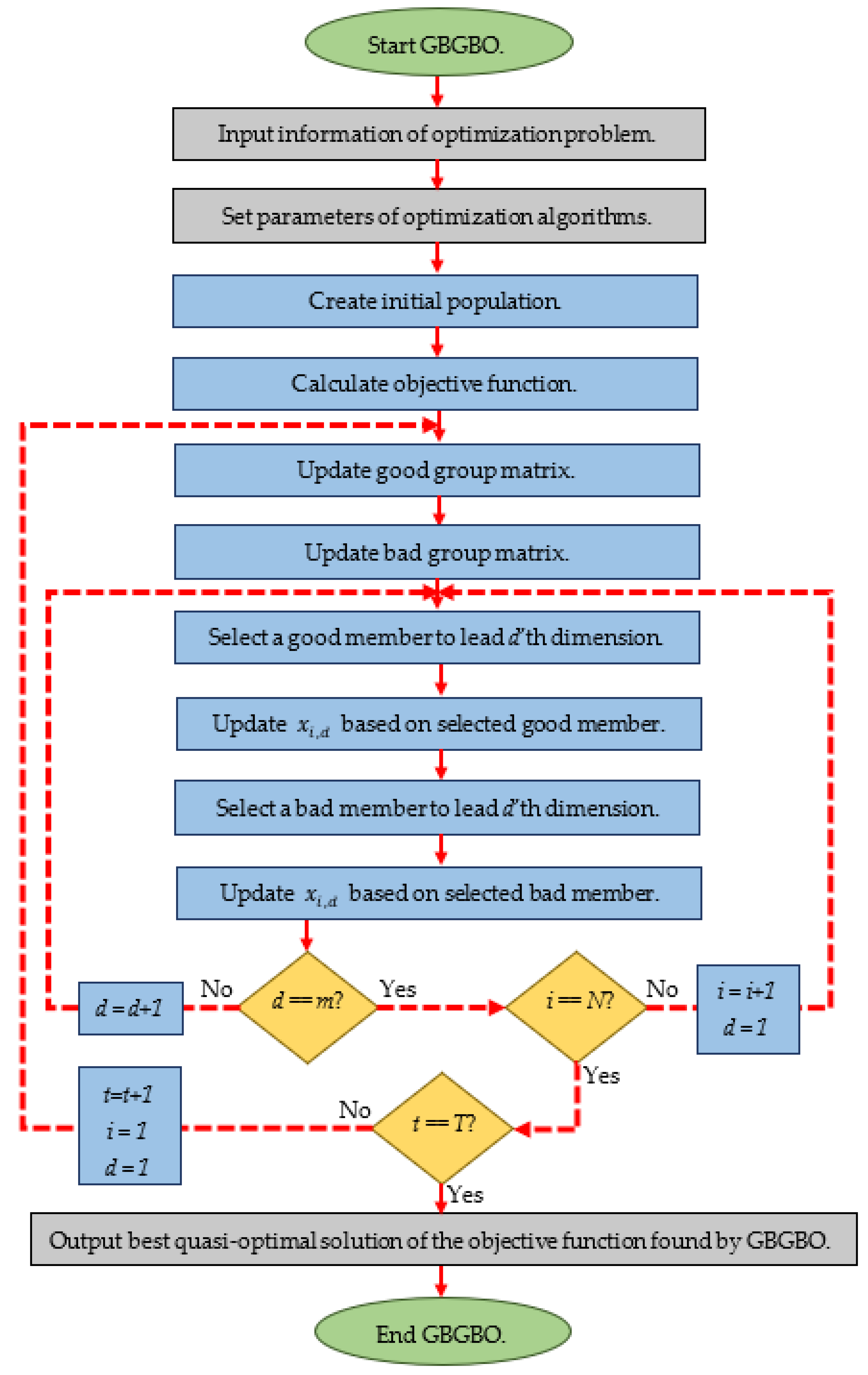
After all variables of all population members were updated based on Equations (5) and (6), the algorithm process was repeated until the stop condition was reached. Then, after the end of the algorithm iterations, the best solution obtained using the BGBGO was presented. Figure 1 shows the implementation of the BGBGO as a flowchart.

3. Simulation and Results

In this section, the performance of the proposed BGBGO algorithm in solving various optimization problems is evaluated. For this purpose, a set of twenty-three standard objective functions including unimodal, high-dimensional multimodal, and fixed-dimensional multimodal functions [16] were optimized using BGBGO. Complete information on these objective functions is given in

Table A1. Unimodal test functions.

$F_1\left(x\right)={{\displaystyle \sum }}_{i=1}^m{x}_i^2$	${\left[-100,100\right]}^m$	m = 30
$F_2\left(x\right)={{\displaystyle \sum }}_{i=1}^m\left|x_i\right|+{{\displaystyle \prod }}_{i=1}^m\left|x_i\right|$	${\left[-10,10\right]}^m$	m = 30
$F_3\left(x\right)={{\displaystyle \sum }}_{i=1}^m{\left({{\displaystyle \sum }}_{j=1}^i{x}_i\right)}^2$	${\left[-100,100\right]}^m$	m = 30
$F_4\left(x\right)=max\left\{\left|x_i\right| , 1\le i\le m \right\}$	${\left[-100,100\right]}^m$	m = 30
$F_5\left(x\right)={{\displaystyle \sum }}_{i=1}^{m-1}\left[100{\left(x_{i+1}-x_i^2\right)}^2+{\left(x_i-1\right)}^2)\right]$	${\left[-30,30\right]}^m$	m = 30
$F_6\left(x\right)={{\displaystyle \sum }}_{i=1}^m{\left(\left[x_i+0.5\right]\right)}^2$	${\left[-100,100\right]}^m$	m = 30
$F_7\left(x\right)={{\displaystyle \sum }}_{i=1}^{m}i{x}_i^4+random\left(0,1\right)$	${\left[-1.28,1.28\right]}^m$	m = 30

,

Table A2. High-dimensional multimodal test functions.

$F_8\left(x\right)={{\displaystyle \sum }}_{i=1}^m-x_i \sin \left(\sqrt{\left|x_i\right|}\right)$	${\left[-500,500\right]}^m$	m = 30
$F_9\left(x\right)={{\displaystyle \sum }}_{i=1}^m\left[ x_i^2-10\cos \left(2\pi x_i\right)+10\right]$	${\left[-5.12,5.12\right]}^m$	m = 30
$F_{10}\left(x\right)=-20\exp \left(-0.2\sqrt{\frac{1}{m}{{\displaystyle \sum }}_{i=1}^m{x}_i^2}\right)-\exp \left(\frac{1}{m}{{\displaystyle \sum }}_{i=1}^m\cos \left(2\pi x_i\right)\right)+20+e$	${\left[-32,32\right]}^m$	m = 30
$F_{11}\left(x\right)=\frac{1}{4000}{{\displaystyle \sum }}_{i=1}^m{x}_i^2-{{\displaystyle \prod }}_{i=1}^{m}cos\left(\frac{x_i}{\sqrt{i}}\right)+1$	${\left[-600,600\right]}^m$	m = 30
$\begin{array}{c}{F}_{12}\left(x\right)=\frac{\pi }{m} \left\{10\sin \left(\pi y_1\right)+{{\displaystyle \sum }}_{i=1}^m{\left(y_i-1\right)}^2\left[1+10{\sin }^2\left(\pi y_{i+1}\right)\right]+{\left(y_n-1\right)}^2\right\}\\ +{{\displaystyle \sum }}_{i=1}^{m}u\left(x_i,10,100,4\right)\end{array}$ $u\left(x_i,a,i,n\right)=\{\begin{array}{c}k{\left(x_i-a\right)}^n, x_i>-a;\\ 0, -a<x_i<a;\\ k{\left(-x_i-a\right)}^n, x_i<-a \end{array}$	${\left[-50,50\right]}^m$	m = 30
$\begin{array}{l}{F}_{13}\left(x\right)=0.1\{{\sin }^2\left(3\pi x_1\right)\\ \hspace{1em}\hspace{1em}\hspace{1em}\hspace{1em}\hspace{1em}\hspace{1em}+{{\displaystyle \sum }}_{i=1}^m{\left(x_i-1\right)}^2\left[1+{\sin }^2\left(3\pi x_i+1\right)\right]+{\left(x_n-1\right)}^2\left[1+{\sin }^2\left(2\pi x_m\right)\right]\}\\ \hspace{1em}\hspace{1em}\hspace{1em}\hspace{1em}\hspace{1em}\hspace{1em}+{{\displaystyle \sum }}_{i=1}^{m}u\left(x_i,5,100,4\right)\end{array}$	${\left[-50,50\right]}^m$	m = 30

and

Table A3. Fixed-dimensional multimodal test functions.

$F_{14}\left(x\right)={\left(\frac{1}{500}+{{\displaystyle \sum }}_{j=1}^{25}\frac{1}{j+{{\displaystyle \sum }}_{i=1}^2{\left(x_i-a_{ij}\right)}^6}\right)}^{-1}$	${\left[-65.53,65.53\right]}^2.$
$F_{15}\left(x\right)={{\displaystyle \sum }}_{i=1}^{11}{\left[a_i-\frac{x_1\left(b_i^2+b_i{x}_2\right)}{b_i^2+b_i{x}_3+x_4}\right]}^2$	${\left[-5,5\right]}^4$
$F_{16}\left(x\right)=4x_1^2-2.1x_1^4+\frac{1}{3}{x}_1^6+x_1{x}_2-4x_2^2+4x_2^4$	${\left[-5,5\right]}^2$
$F_{17}\left(x\right)={\left(x_2-\frac{5.1}{4{\pi }^2}{x}_1^2+\frac{5}{\pi }{x}_1-6\right)}^2+10\left(1-\frac{1}{8\pi }\right)cos{x}_1+10$	[−5,10] $\times$ [0,15]
$\begin{array}{c}{F}_{18}\left(x\right)=\left[1+{\left(x_1+x_2+1\right)}^2\left(19-14x_1+3x_1^2-14x_2+6x_1{x}_2+3x_2^2\right)\right]\\ \times \left[30+{\left(2x_1-3x_2\right)}^2\times \left(18-32x_1+12x_1^2+48x_2-36x_1{x}_2+27x_2^2\right)\right]\end{array}$	${\left[-5,5\right]}^2$
$F_{19}\left(x\right)=-{{\displaystyle \sum }}_{i=1}^4{c}_i\exp \left(-{{\displaystyle \sum }}_{j=1}^3{a}_{ij}{\left(x_j-P_{ij}\right)}^2\right)$	${\left[0,1\right]}^3$
$F_{20}\left(x\right)=-{{\displaystyle \sum }}_{i=1}^4{c}_i\exp \left(-{{\displaystyle \sum }}_{j=1}^6{a}_{ij}{\left(x_j-P_{ij}\right)}^2\right)$	${\left[0,1\right]}^6$
$F_{21}\left(x\right)=-{{\displaystyle \sum }}_{i=1}^5{\left[\left(X-a_i\right){\left(X-a_i\right)}^T+6c_i\right]}^{-1}$	${\left[0,10\right]}^4$
$F_{22}\left(x\right)=-{{\displaystyle \sum }}_{i=1}^7{\left[\left(X-a_i\right){\left(X-a_i\right)}^T+6c_i\right]}^{-1}$	${\left[0,10\right]}^4$
$F_{23}\left(x\right)=-{{\displaystyle \sum }}_{i=1}^{10}{\left[\left(X-a_i\right){\left(X-a_i\right)}^T+6c_i\right]}^{-1}$	${\left[0,10\right]}^4$

in Appendix A. Eight optimization algorithms, including the genetic algorithm (GA) [15], particle swarm optimization (PSO) [6], gravitational search algorithm (GSA) [5], teaching–learning-based optimization (TLBO) [8], gray wolf optimizer (GWO) [10], whale optimization algorithm (WOA) [9], tunicate swarm algorithm (TSA) [11], and marine predators algorithm (MPA) [12], were investigated in order to compare the optimization results. The experimentation was performed on MATLAB (version R2020a) using a 64-bit Core i7 processor with 3.20 GHz and 16 GB of main memory. Each of the optimization algorithms were independently implemented twenty times, and at the end the optimization results were presented as the mean and standard deviation of the best solutions as “ave” and “std”.

The values used for the main controlling parameters of the comparative algorithms are specified in

Table 1. Parameter values for the comparative algorithms.

Algorithm	Parameter	Value
GA
	Type	Real coded
	Selection	Roulette wheel (Proportionate)
	Crossover	Whole arithmetic (Probability = 0.8, $\alpha =\left[-0.5, 1.5\right]$)
	Mutation	Gaussian (Probability = 0.05)
PSO
	Topology	Fully connected
	Cognitive and social constant	(C1, C2) 2, 2
	Inertia weight	Linear reduction from 0.9 to 0.1
	Velocity limit	10% of dimension range
GSA
	Alpha, G0, Rnorm, Rpower	20, 100, 2, 1
TLBO
	TF: teaching factor	TF = round $\left[\left(1+rand\right)\right]$
	random number	rand$\mathrm{is}\mathrm{a}\mathrm{random}\mathrm{number}\mathrm{in}\left[0, 1\right].$
GWO
	Convergence parameter (a)	a: Linear reduction from 2 to 0.
WOA
	Convergence parameter (a)	a: Linear reduction from 2 to 0.
	r$\mathrm{is}\mathrm{a}\mathrm{random}\mathrm{vector}\mathrm{in}\left[0,1\right].$
	l$\mathrm{is}\mathrm{a}\mathrm{random}\mathrm{number}\mathrm{in}\left[-1,1\right].$
TSA
	Pmin and Pmax	1, 4
	c1, c2, c3	Random numbers lie in the range from 0 to 1.
MPA
	Constant number	p = 0.5
	Random vector	R$\mathrm{is}\mathrm{a}\mathrm{vector}\mathrm{of}\mathrm{uniform}\mathrm{random}\mathrm{numbers}\mathrm{in}\left[0, 1\right].$
	Fish Aggregating Devices (FADs)	FADS = 0.2
	Binary vector	U = 0 or 1

.

3.1. Simulation Results on Unimodal Test Function F₁ to F₇

Seven objective functions F₁ to F₇ were selected as unimodal objective functions to evaluate the performance of the GBGBO and other algorithms. Complete information on these objective functions is given in Table A1 in Appendix A. These objective functions had only one optimal solution and were therefore suitable for evaluating the exploitation power of optimization algorithms. The results of the optimization of these objective functions after twenty independent implementations are presented in

Table 2. Optimization results of GBGBO and other algorithms on unimodal test function.

		GA	PSO	GSA	TLBO	GWO	GOA	TSA	MPA	GBGBO
F1	Ave	13.2405	1.7740 × 10−5	2.0255 × 10−17	8.3373 × 10−60	1.09 × 10−58	2.1741 × 10−9	7.71 × 10−38	3.2715 × 10−21	3.2429 × 10−121
	std	4.7664 × 10−15	6.4396 × 10−21	1.1369 × 10−32	4.9436 × 10−76	5.1413 × 10−74	7.3985 × 10−25	7.00 × 10−21	4.6153 × 10−21	4.8 × 10−138
F2	Ave	2.4794	0.3411	2.3702 × 10−8	7.1704 × 10−35	1.2952 × 10−34	0.5462	8.48 × 10−39	1.57 × 10−12	8.51 × 10−65
	std	2.2342 × 10−15	7.4476 × 10−17	5.1789 × 10−24	6.6936 × 10−50	1.9127 × 10−50	1.7377 × 10−16	5.92 × 10−41	1.42 × 10−12	1.66 × 10−79
F3	Ave	1536.8963	589.492	279.3439	2.7531 × 10−15	7.4091 × 10−15	1.7634 × 10−8	1.15 × 10−21	0.0864	4.45 × 10−64
	std	6.6095 × 10−13	7.1179 × 10−13	1.2075 × 10−13	2.6459 × 10−31	5.6446 × 10−30	1.0357 × 10−23	6.70 × 10−21	0.1444	4.15 × 10−74
F4	Ave	2.0942	3.9634	3.2547 × 10−9	9.4199 × 10−15	1.2599 × 10−14	2.9009 × 10−5	1.33 × 10−23	2.6 × 10−8	1.22 × 10−55
	std	2.2342 × 10−15	1.9860 × 10−16	2.0346 × 10−24	2.1167 × 10−30	1.0583 × 10−29	1.2121 × 10−20	1.15 × 10−22	9.25 × 10−9	2.27 × 10−70
F5	Ave	310.4273	50.26245	36.10695	146.4564	26.8607	41.7767	28.8615	46.049	27.02145
	std	2.0972 × 10−13	1.5888 × 10−14	3.0982 × 10−14	1.9065 × 10−14	0	2.5421 × 10−14	4.76 × 10−3	0.4219	3.97 × 10−15
F6	Ave	14.55	20.25	0	0.4435	0.6423	1.6085 × 10−9	7.10 × 10−21	0.398	0
	std	3.1776 × 10−15	1.2564	0	4.2203 × 10−16	6.2063 × 10−17	4.6240 × 10−25	1.12 × 10−25	0.1914	0
F7	Ave	5.6799 × 10−3	0.1134	0.0206	0.0017	0.0008	0.0205	3.72 × 10−4	0.0018	3.3919 × 10−5
	std	7.7579 × 10−19	4.3444 × 10−17	2.7152 × 10−18	3.87896 × 10−19	7.2730 × 10−20	1.5515 × 10−18	5.09 × 10−5	0.001	2.67 × 10−19

. The optimization results of these objective functions showed that the proposed GBGBO offered better solutions than other algorithms. This indicates that the GBGBO had a high exploitation power in achieving the optimal solution.

3.2. Simulation Results on High Dimensional Multi Modal Test Function F₈ to F₁₃

The second group of objective functions to evaluate optimization algorithms are the high dimensional multimodal test function. The six target functions F₈ to F₁₃ are of this type. Complete information on these objective functions is given in Table A2 in Appendix A. These types of objective functions are several local optimal solutions and were therefore suitable for evaluating the exploration power of the optimization algorithms. The results of the optimization of these objective functions are presented in

Table 3. Optimization results of GBGBO and other algorithms on high dimensional test function.

E		GA	PSO	GSA	TLBO	GWO	GOA	TSA	MPA	GBGBO
F8	Ave	−8184.4142	−6908.6558	−2849.0724	−7408.6107	−5885.1172	−1663.9782	−5740.3388	−3594.16321	−4548.05
	std	833.2165	625.6248	264.3516	513.5784	467.5138	716.3492	41.5	811.32651	1.02 × 10−12
F9	Ave	62.4114	57.0613	16.2675	10.2485	8.5265 × 10−15	4.2011	5.70 × 10−3	140.1238	0
	std	2.5421 × 10−14	6.3552 × 10−15	3.1776 × 10−15	5.5608 × 10−15	5.6446 × 10−30	4.3692 × 10−15	1.46 × 10−3	26.3124	0
F10	Ave	3.2218	2.1546	3.5673 × 10−9	0.2757	1.7053 × 10−14	0.3293	9.80 × 10−14	9.6987 × 10−12	4.44 × 10−15
	std	5.1636 × 10−15	7.9441 × 10−16	3.6992 × 10−25	2.5641 × 10−15	2.7517 × 10−29	1.9860 × 10−16	4.51 × 10−12	6.1325 × 10−12	1.41 × 10−30
F11	Ave	1.2302	0.0462	3.7375	0.6082	0.0037	0.1189	1.00 × 10−7	0	0
	std	8.4406 × 10−16	3.1031 × 10−18	2.7804 × 10−15	1.9860 × 10−16	1.2606 × 10−18	8.9991 × 10−17	7.46 × 10−7	0	0
F12	Ave	0.047	0.4806	0.0362	0.0203	0.0372	1.7414	0.0368	0.0851	1.60 × 10−4
	std	4.6547 × 10−18	1.8619 × 10−16	6.2063 × 10−18	7.7579 × 10−19	4.3444 × 10−17	8.1347 × 10−12	1.5461 × 10−2	0.0052	2.17 × 10−17
F13	Ave	1.2085	0.5084	0.002	0.3293	0.5763	0.3456	2.9575	0.4901	1.08 × 10−4
	std	3.2272 × 10−16	4.9650 × 10−17	4.2617 × 10−14	2.1101 × 10−16	2.4825 × 10−16	3.25391 × 10−12	1.5682 × 10−12	0.1932	2.98 × 10−16

. These results indicate the ability of the GBGBO to solve these types of objective functions and the superiority of the proposed algorithm over other algorithms. Therefore, the GBGBO had good exploration capability and scanned the search space of the problem well.

3.3. Simulation Results on Fixed Dimensional Multi Modal Test Function F₁₄ to F₂₃

The third group of objective functions, including F₁₄ to F₂₃, was selected from the fixed dimensional multimodal type. Complete information on these objective functions is given in Table A3 in Appendix A. This type of objective function was also suitable for evaluating the exploration power of optimization algorithms. The results of optimization of these objective functions using GBGBO and eight other algorithms are presented in

Table 4. Optimization results of GBGBO and other algorithms on fixed dimensional test function.

E		GA	PSO	GSA	TLBO	GWO	GOA	TSA	MPA	GBGBO
F14	Ave	0.9986	2.1735	3.5913	2.2721	3.7408	0.998	1.9923	0.998	0.998
	std	1.5640 × 10−15	7.9441 × 10−16	7.9441 × 10−16	1.9860 × 10−16	6.4545 × 10−15	9.4336 × 10−16	2.6548 × 10−7	4.2735 × 10−16	1.44 × 10−16
F15	Ave	5.3952 × 10−2	0.0535	0.0024	0.0033	0.0063	0.0049	0.0004	0.003	0.0003
	std	7.0791 × 10−18	3.8789 × 10−19	2.9092 × 10−19	1.2218 × 10−17	1.1636 × 10−18	3.4910 × 10−18	9.0125 × 10−4	4.0951 × 10−15	3.64 × 10−20
F16	Ave	−1.0316	−1.0316	−1.0316	−1.0316	−1.0316	−1.0316	−1.0316	−1.0316	−1.0316
	std	7.9441 × 10−16	3.4755 × 10−16	5.9580 × 10−16	1.4398 × 10−15	3.9720 × 10−16	9.9301 × 10−16	2.6514 × 10−16	4.4652 × 10−16	9.93 × 10−17
F17	Ave	0.4369	0.7854	0.3978	0.3978	0.3978	0.4047	0.3991	0.3979	0.3979
	std	4.9650 × 10−17	4.9650 × 10−17	9.9301 × 10−17	7.4476 × 10−17	8.6888 × 10−17	2.4825 × 10−17	2.1596 × 10−16	9.1235 × 10−15	9.93 × 10−17
F18	Ave	4.3592	3	3	3.0009	3	3	3	3	3
	std	5.9580 × 10−16	3.6741 × 10−15	6.9511 × 10−16	1.5888 × 10−15	2.0853 × 10−15	5.6984 × 10−15	2.6528 × 10−15	1.9584 × 10−15	1.99 × 10−16
F19	Ave	−3.85434	−3.8627	−3.8627	−3.8609	−3.8621	−3.8627	−3.8066	−3.8627	−3.8627
	std	9.9301 × 10−17	8.9371 × 10−15	8.3413 × 10−15	7.3483 × 10−15	2.4825 × 10−15	3.1916 × 10−15	2.6357 × 10−15	4.2428 × 10−15	4.97 × 10−16
F20	Ave	−2.8239	−3.2619	−3.0396	−3.2014	−3.2523	−3.2424	−3.3206	−3.3211	−3.3219
	std	3.97205 × 10−16	2.9790 × 10−16	2.1846 × 10−14	1.7874 × 10−15	2.1846 × 10−15	7.9441 × 10−16	5.6918 × 10−15	1.1421 × 10−11	2.88 × 10−15
F21	Ave	−4.3040	−5.3891	−5.1486	−9.1746	−9.6452	−7.4016	−5.5021	−10.1532	−10.1532
	std	1.5888 × 10−15	1.4895 × 10−15	2.9790 × 10−16	8.5399 × 10−15	6.5538 × 10−15	2.3819 × 10−11	5.4615 × 10−13	2.5361 × 10−11	7.94 × 10−16
F22	Ave	−5.1174	−7.6323	−9.0239	−10.0389	−10.4025	−8.8165	−5.0625	−10.4029	−10.4029
	std	1.2909 × 10−15	1.5888 × 10−15	1.6484 × 10−12	1.5292 × 10−14	1.9860 × 10−15	6.7524 × 10−15	8.4637 × 10−14	2.8154 × 10−11	7.15 × 10−15
F23	Ave	−6.5621	−6.1648	−8.9045	−9.2905	−10.1302	−10.0003	−10.3613	−10.5364	−10.5364
	std	3.8727 × 10−15	2.7804 × 10−15	7.1497 × 10−14	1.1916 × 10−15	4.5678 × 10−15	9.1357 × 10−15	7.6492 × 10−12	3.9861 × 10−11	7.94 × 10−16

. What is clear from these results is that the proposed GBGBO algorithm performed very well in such objective functions and in most cases provided the global optimal solution. This concept demonstrates the acceptable exploration ability of the GBGBO in accurately searching the problem search space.

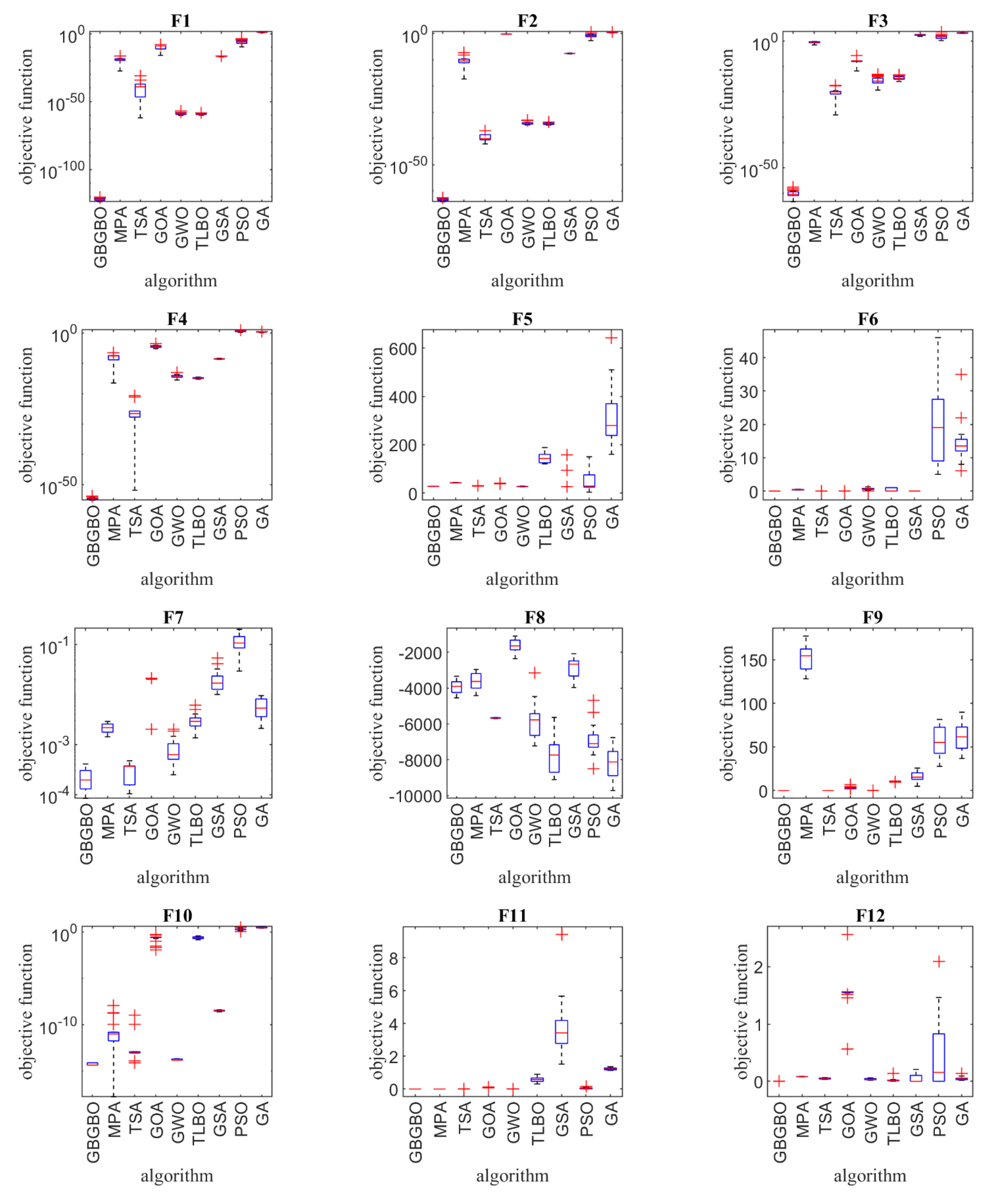
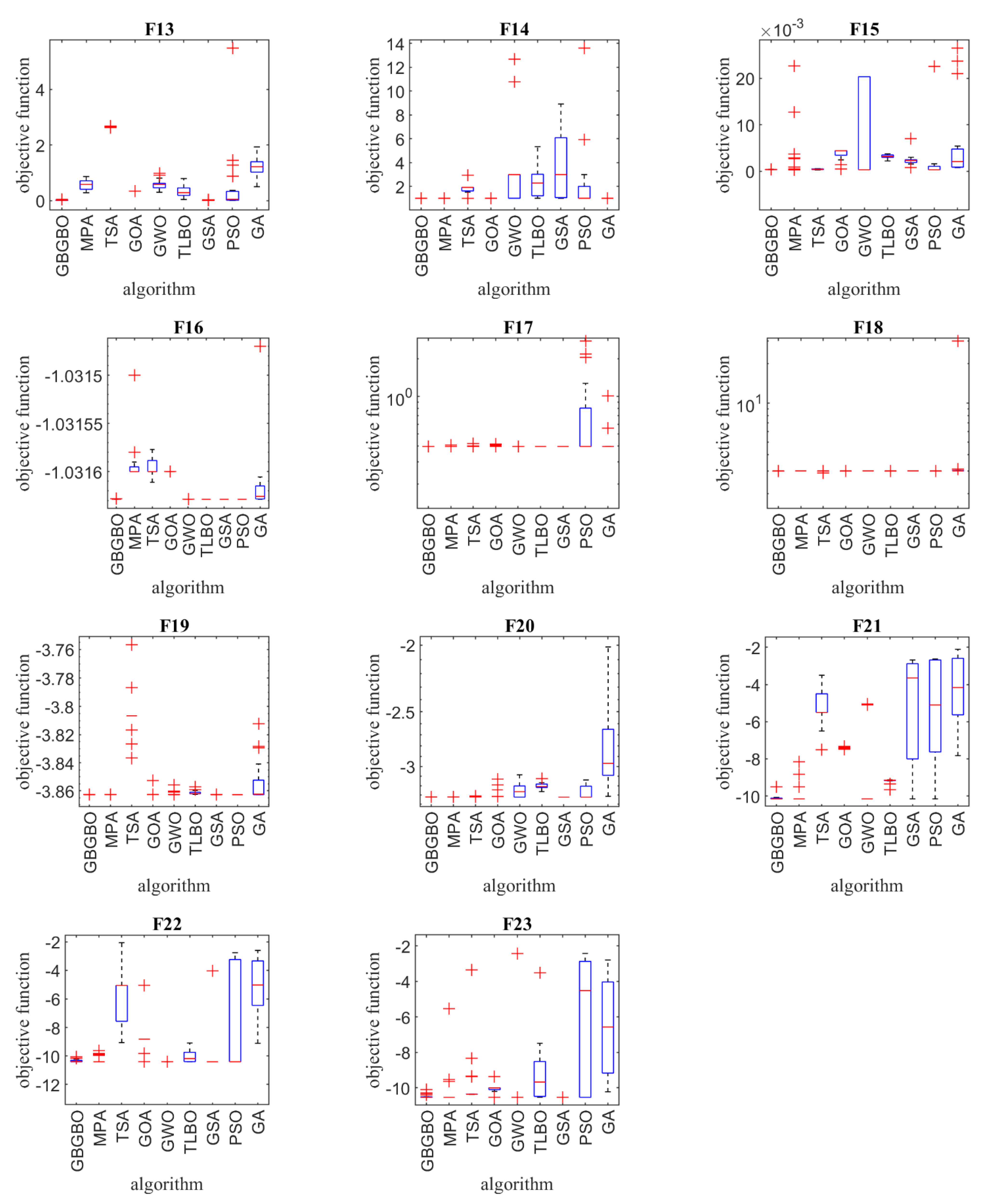
Optimization results of the F₁ to F₂₃ objective functions using the proposed algorithm and eight other optimization algorithms are presented in Table 2, Table 3 and Table 4. The boxplot of results for each algorithm and objective function are drawn in Figure 2 for further analysis and visual comparison of the performance of the optimization algorithms. Based on the boxplots shown in Figure 2, in the unimodal objective functions type F₁, F₂, F₃, F₄, F₆, and F₇, the superiority of the GBGBO over the other eight algorithms is obvious. The function F₅ of the GWO offers better performance. However, the GBGBO offers acceptable performance with little difference to the GWO. In the functions F₉, F₁₀, F₁₁, F₁₂, and F₁₃ of the high-dimensional multimodal objective functions type, the GBGBO is the best optimizer among the review algorithms. In the objective function F₈, the GA presented better performance. In the functions F₁₄, F₁₅, F₁₆, F₁₈, F₁₉, F₂₀, F₂₁, F₂₂, and F₂₃ of the fixed-dimensional multi-model objective function type, the proposed algorithm could provide a more efficient quasi-optimal solution with smaller values of standard deviation. The function F₁₇ in the GWO offers better performance. However, the GBGBO offers acceptable performance with little difference to the GWO.

4. Statistical Analysis

The optimization results of all three types of objective functions were presented as the mean and standard deviation of the solutions. Although these indicators make important information available, they alone were not enough to ensure that one algorithm is superior to other algorithms. This is because even after twenty independent executions, the superiority of one optimization algorithm over other algorithms may occur randomly, even with the lowest probability. Thus, a statistical analysis of the optimization results provided more information than the capability of an optimization algorithm. In this article, the Friedman rank test [17] was used. The results of this test are determined in

Table 5. Results of Friedman rank test.

Test Function			GA	PSO	GSA	TLBO	GWO	GOA	TSA	MPA	GBGBO.
1	Unimodal	Friedman value	56	55	37	27	24	41	16	36	8
	(F1–F7)	Friedman rank	9	8	6	4	3	7	2	5	1
2	High dimensional multimodal	Friedman value	37	34	30	22	21	36	24	32	11
	(F8–F13)	Friedman rank	8	6	4	3	2	7	3	5	1
3	Fixed dimension multimodal	Friedman value	56	48	42	37	33	37	35	23	11
	(F14–F23)	Friedman rank	8	7	6	5	3	5	4	2	1
4	All 23-test function	Friedman value	149	137	109	86	78	114	75	91	30
		Friedman rank	9	8	6	4	3	7	2	5	1

. Analysis and comparison of these results show that BGBGO performs better than other algorithms in all three different types of objective functions unimodal, high dimensional multimodal, and fixed dimensional multimodal. In addition, the result of analysis on all twenty-three objective functions shows that the GBGBO ranks first among compared algorithms.

5. Discussion

Exploitation and exploration indexes are two important criteria and indicators in analyzing and evaluating the performance of optimization algorithms. The exploitation power means the ability of an optimization algorithm to provide a suitable quasi-optimal solution at the end of the algorithm iterations. Thus, in comparing the performance of several optimization algorithms on an optimization problem, the algorithm that can ultimately provide a quasi-optimal solution closer to the global optimal has higher exploitation power. The unimodal objective functions F₁ to F₇ have only one main solution and are therefore very suitable for evaluating the exploitation power of optimization algorithms. Comparison of the optimization results of these functions using the GBGBO and eight other algorithms in Table 2 shows the acceptable exploitation power of the GBGBO in solving optimization problems. Exploration power means the ability of an algorithm to accurately scan the search space of the optimization problem. In fact, among several optimization algorithms, an algorithm that can scan the search space well and is not limited to certain areas, as well as can pass locally optimal solutions, has higher exploration power. This indicator is especially important for optimization problems that have multiple local optimal solutions. The F₈ to F₂₃ objective functions had several local optimal solutions in addition to the main solution. Therefore, these objective functions were suitable for evaluating the exploration power of optimization algorithms. Analysis and comparison of the optimization results of the GBGBO and eight other algorithms on these objective functions, which are presented in Table 3 and Table 4, indicated the acceptable exploration power of the proposed GBGBO algorithm in solving this type of objective functions. On the other hand, the results of the Friedman rank test showed that the acceptable power of the GBGBO in exploration and exploitation indices is not random.

6. Conclusions and Future Work

Optimization algorithms are one of the efficient tools in solving optimization problems. Optimization algorithms with random search space scanning are able to provide quasi-optimal solutions to optimization problems. In this paper, a new optimization algorithm called the good and bad groups-based optimizer (GBGBO) was presented to solve optimization problems. The GBGBO was designed based on simulation of the process of guiding the population members by two groups named good and bad groups, instead of only the best and worst members. The proposed GBGBO was mathematically modeled. The performance of the GBGBO was implemented and evaluated on a set of twenty-three standard objective functions. These objective functions were selected in three different types unimodal to evaluate exploitation power, high-dimensional, and fixed-dimensional multimodal to evaluate exploration power. Eight optimization algorithms, concretely the genetic algorithm (GA), the particle swarm optimization (PSO), the gravitational search algorithm (GSA), the teaching–learning-based optimization (TLBO), the gray wolf optimizer (GWO), the whale optimization algorithm (WOA), the tunicate swarm algorithm (TSA), and the marine predators algorithm (MPA), were selected to compare with the optimization results obtained from the GBGBO. The optimization results showed that the GBGBO is more capable of solving optimization problems than the other eight optimization algorithms and is more competitive. In addition, the Friedman rank test was used for statistical analysis of optimization results provided by optimization algorithms. Based on the results of this test, the GBGBO had a good performance in solving optimization problems and was ranked first among the compared algorithms.

The authors suggest some ideas and perspectives for future studies. The design of the binary version, as well as the multi-objective version of the GBGBO, are two special potentials for this study. Apart from this, implementing the GBGBO on various optimization problems and real-world optimization problems could be some significant contributions as well.