A Study on the Errors of 2D Circular Trajectories Generated on a 3D Printer

Abstract

This paper presents a study on the movement precision and accuracy of an extruder system related to the print bed on a 3D printer evaluated using the features of 2D circular trajectories generated by simultaneous displacement on x and y-axes. A computer-assisted experimental setup allows the sampling of displacement evolutions, measured with two non-contact optical sensors. Some processing procedures of the displacement signals are proposed in order to evaluate and to describe the circular trajectories errors (e.g., open and closed curves fitting, the detection of recurrent periodical patterns in x and y-motions, low pass numerical filtering, etc.). The description of these errors is suitable to certify that the 3D printer works correctly (keeping the characteristics declared by the manufacturer) for maintenance purpose sand, especially, for computer-aided correction of accuracy (e.g., by error compensation).

1. Introduction

The additive fabrication is a common topic in various domains of activity (industry, biology, medicine). The compliance with precision conditions of 3D-printed parts (shape and dimensions tolerances, surface quality, etc.) becomes more and more a critical issue. Their use in some technical applications where precision and accuracy (P&A) are required is severely restricted since, for the present, other manufacturing technologies offer better results. Many studies in engineering and scientific research are focused on ensuring the P&A of 3D printers by error avoidance [1]. Other studies are involved in experimental research (measurements and data processing) in order to verify and to correct the errors generated by the lack of P&A on 3D printers by error compensation [1].

There are many issues involved in the appearance of errors in additive fabrication. Not surprisingly, some of them are not related with the 3D printer features (e.g., structure, P&A of kinematics, dynamics, position control, deposition process, temperature, etc.). For example, in [2] is established that the accuracy of STL (.stl) files (from Standard Tessellation Language or Standard Triangle Language, commonly used by Fused Deposition Modelling on 3D printers) essentially depends on the design of 3D CAD models (six different CAD systems generate STL files with different accuracies). In [3], is established that the conversion in STL format is done with errors by some CAD software products. The software interface used to drive the printer (slicer software, establishing the way the model is built) is often a source of inaccuracy [4] when inappropriate values of setting parameters are suggested by the software and accepted by user [5].

Sometimes the CAD models are generated with errors (and these errors are transferred to the printed object), especially when these models are generated as a virtual copy of a real object, e.g., by imaging, segmentation, and post processing of medical models [6,7] or by reverse engineering using a 3D-scanning and design process [8,9].

Some sources of errors are related to material deposition during additive manufacturing (e.g., flow properties) as susceptible to random variations [5]. The effect of print layer height on the accuracy of orthodontic models is considered in [10]. The effect of orientation (effect of gravity) and the effect of the support are investigated by [1]. A study on the influence of the accuracy related to size/position of printed benchmarks and the position of working planes on 3D printers is revealed in [11].The influence on P&A and mechanical properties (measured by tensile test) of a specimen object related to the print position of a specimen object is presented in [12,13].

The influence of different common printing technologies on the accuracy of mandibular models was considered in the research results shown in [14]. The influence of different types of thermoplastic filament materials used in additive fabrication on surface roughness was evaluated in [15].

The evolution in time of internal material tension, dimension and shape (by aging) as source of errors in 3D printing is a topic studied in [16]. A simple method to appreciate the P&A of 3D printers (and to calibrate it as well) is the measurement of a printed object (the most common being “#3D Benchy” from Creative Tools) or the quality of a printed structure (e.g.,“#All in one test 3D printer”). In [17], an insitu measurement method (by the scanning of layers) during the additive manufacturing process is proposed. The use of a coordinate measurement machine is proposed to describe the accuracy of medical models in [18,19]) and the optical scanning is mentioned in [6]). A metrology feedback procedure is used in [20,21] to improve the geometrical accuracy by errors compensation using a 3D scanning on sacrificial printed objects.

The displacement errors and the errors of the relative position of movable parts are often related by kinematics of a 3D printer. Frequently, the contouring errors due to axis misalignment (also a relevant topic, investigated in our study) are involved in a bad P&A. The measurement of these errors and their compensation in the computer numerical control system of the printer is a major challenge in improving the additive fabrication performances. Thus, in [22] is proposed a simple compensation model for kinematic errors based on measurement results done on the printer using a Renishaw QC10 ball bar device (from Renishaw, UK). For the 3D printers based on parallel robotic systems, in [23,24] some theoretical kinematic error models useful in automatic compensation are proposed. A volumetric experimental compensation technique for kinematic errors is exposed in [25]. In order to minimize the tracking errors of desired trajectories, a feed forward control procedure is proposed in [26].

This brief study of the literature reveals that few reports are focused on non-contact measurement methods of the errors produced by the kinematics of a 3D printer during complex motions of the extruder related to the print bed (especially 2D closed trajectories).

Our approach on this paper was based on this obvious remark: the open-loop computer-aided control of each of three motions of a printer (usually 3D printers don’t use feedback control related to real position) is vulnerable to some uncontrollable (constant or variable) phenomena generated by mechanical parts (elastic deformations in toothed belts, mechanical backlashes, hysteresis behaviour, errors in lead screw threads, variation of friction forces in axes carriages, mechanical wear, structural vibrations induced by stepper motors, etc.). Because the 3D printing is achieved by deposition of material layer by layer (in a horizontal plane), an important characterization of P&A for any printer should be done by the P&A displacement, position and, especially, of 2D complex closed trajectories with the printer running in absence of the printing process. On this line of thinking we consider that a circular trajectory (of the extruder system related to the print bed) is one of the best theoretical approaches mainly because two simultaneous, strictly correlated linear motions are involved (on the x and y-axis). With a constant speed on the circular trajectory, these motions should be described by two almost identical harmonic evolutions (except the π/2 phase shift between), with periodic changes of the position, direction, speed and acceleration. An important argument for our approach based on circular trajectories is this one: the 2D circular trajectories are systematically involved in ISO standards methods for P&A evaluation of CNC manufacturing systems (ISO 230-4, [27]).

The benefits of this approach with 2D circular trajectories in P&A evaluation is confirmed by the work from [22].

In addition, from an experimental point of view, it is appropriate to work with circular trajectories generated by two simultaneous, simple harmonic linear motions (cosine motion of the extruder system on the x-axis, sine motion of the print bed on the y-axis) measured with a computer-assisted experimental setup based on two optical (non-contact) position sensors. We consider that this is a better approach, in contrast with the measurement system proposed in [22], which uses a ball bar measurement device placed between the extruder and the print bed. Because of this device, the relative motion of the extruder related to the print bed is not totally free.

The Section 2 of this paper presents the computer-aided experimental measurement setup, the Section 3 presents the theoretical and experimental considerations and comments related with the results (signal processing and P&A estimation, based mainly on real trajectory circular fitting), and the Section 4 is dedicated to conclusions and future work.

2. Experimental Setup

The experimental research was done on an Anet A8 3D printer [28], previously used in additive manufacturing for 230 operating hours. The 3D printer has the print bed movable on the y-axis, while the extruder system moves along the x and z-axes independently. On the x-axis, motion is numerically controlled (in open loop) via a stepper motor and a toothed belt (similarly on the y-axis); on the z-axis, the motion is controlled (in open loop) with two synchronized stepper motors with screw-nut systems. The absolute displacement measurement on the y-axis is done with a non-contact ILD 2000-20 [29] laser triangulation sensor (from MICRO-EPSILON MESSTECHNIK GmbH & Co, Ortenburg, Germany) with 20 mm measurement range (1 μm resolution and 10,000 s⁻¹ sampling rate) with the laser beam placed perpendicularly on the target (the print bed) as Figure 1 indicates. Here the point of incidence is placed in the center of the red rectangle. An identical sensor is firmly placed on the print bed, with the laser beam placed perpendicularly to the extruder system (which moves as a sensor target in x-direction), as Figure 2 indicates.

The signals generated by these sensors are two voltages proportional with the displacements (with 1.975 mm/V as proportionality factor for the x-axis sensor and 2.0185 mm/V for the y-axis sensor) related to the middle of the measurement range.

These signals are simultaneously numerically described (by sampling and data acquisition)with a PicoScope 4824 numerical oscilloscope (from PicoTechnology UK, 8 channels, 12 bits, 80 MS/s maximum sampling rate, 256 MS memory) and delivered in numerical format to a computer for processing and analysis. Figure 3 presents a scheme of the computer-assisted experimental setup with only the movable parts of the 3D printer involved in 2D circular trajectories (the extruder and the print bed), the optical sensors for x and y-motion non-contact measurement, the power supply for sensors, the numerical oscilloscope and the computer.

Using an appropriate programming of the drive system written in G-code, the 3D printer was programmed to generate some identical repetitive circular trajectories of the extruder system related to the print bed (with 8.987 mm radius, each one covered in 8.987 s) for 50 s (for almost 5.5 complete trajectories). There are not special reasons to have this coincidence of values for radius and time, except the fact that these values should be accurately found by curve fitting (with the sine model) of the motions involved in the achieving of circular trajectory. However, these values assure a relatively small speed on the 2D circular trajectory. These trajectories are generated using two theoretical pure harmonic motions (x-motion accomplished by the extruder system, y-motion accomplished by the print bed) on the x and y-axes (both having a period T of 8.987 s), experimentally revealed by the computer measurement setup, as a detail in Figure 4 indicates. Here the blue-colored curve describes the motion on the x-axis; the one colored in red describes the motion on y-axis, both with 20,000 s⁻¹ sampling rate. The choosing of this sampling rate is based on this argument: it should be at least two times bigger than the sampling rate of the sensors (10,000 s⁻¹). The sampling rate of the sensors acts as the Nyquist frequency for the sampling rate of the oscilloscope. It is not difficult to remark the resources of these two simultaneous evolutions for P&A evaluation. In Figure 5, a zoomed in detail in area A of Figure 4 proves that each of two real x and y-motions are not strictly pure, simple harmonic shapes (especially the y-motion). As a result, in a summary valuation, the trajectory of the extruder system related to the print bed does not have a strictly circular shape as expected.

These two evolutions are useful for P&A evaluation of the circular trajectories on a 3D printer in experimental terms. For this purpose, some different techniques of computer-aided signal processing will be applied (e.g., the recurrent periodical pattern detection on x and y-motion, curve fitting, circular fitting, low pass numerical filtering).

3. Experimental Results and Discussion

There are many important exploitable resources of x and y-motions description already partially revealed in Figure 4 and Figure 5. As a first interesting approach, we propose the signals fitting, each one with a single harmonic function (fitting with a sine model). The Curve Fitting Tool from Matlab provides the best analytical approximation x_a and y_a of x and y-motion, as follows:

$$x_a\left(t\right)=8.987·\sin \left(0.6991·t+1.398\right)y_a\left(t\right)=8.987·\sin \left(0.6991·t-0.1883\right)$$

(1)

The fitting quality is confirmed for both motions by the same amplitude (8.987 mm, this being the radius of the circular trajectory) and angular frequency ω = 0.6991 rad/s (for a period T = 2π/ω = 8.987 s). These values found by curve fitting were already used in circular trajectory programming. However, there is a shift of phase by 1.5863 radians between motions (1.5863 > π/2 = 1.5707). This means that the x and y-axes are not rigorously perpendicular (there is an axes misalignment), as a first indicator for the lack of P&A. The printer works in a non-orthogonal x0y system (with an angle of 90.893 degrees between axes). As a result, a programmed circular trajectory will be executed as an elliptical one. Nevertheless, this non-perpendicularity of x and y-axes revealed here can be compensated by programming. In a short definition, this compensation should solve this question: what kind of elliptical trajectory should be programmed in order to achieve a desired circular trajectory?

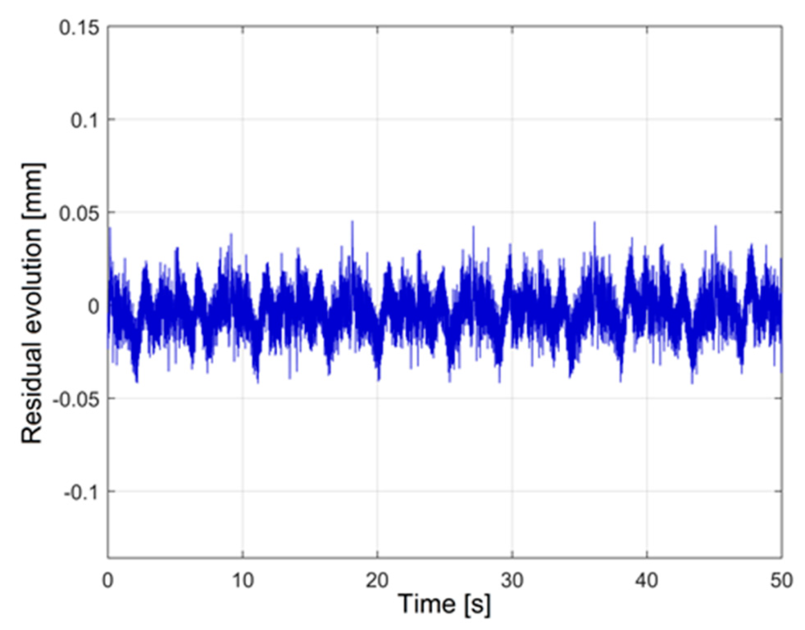
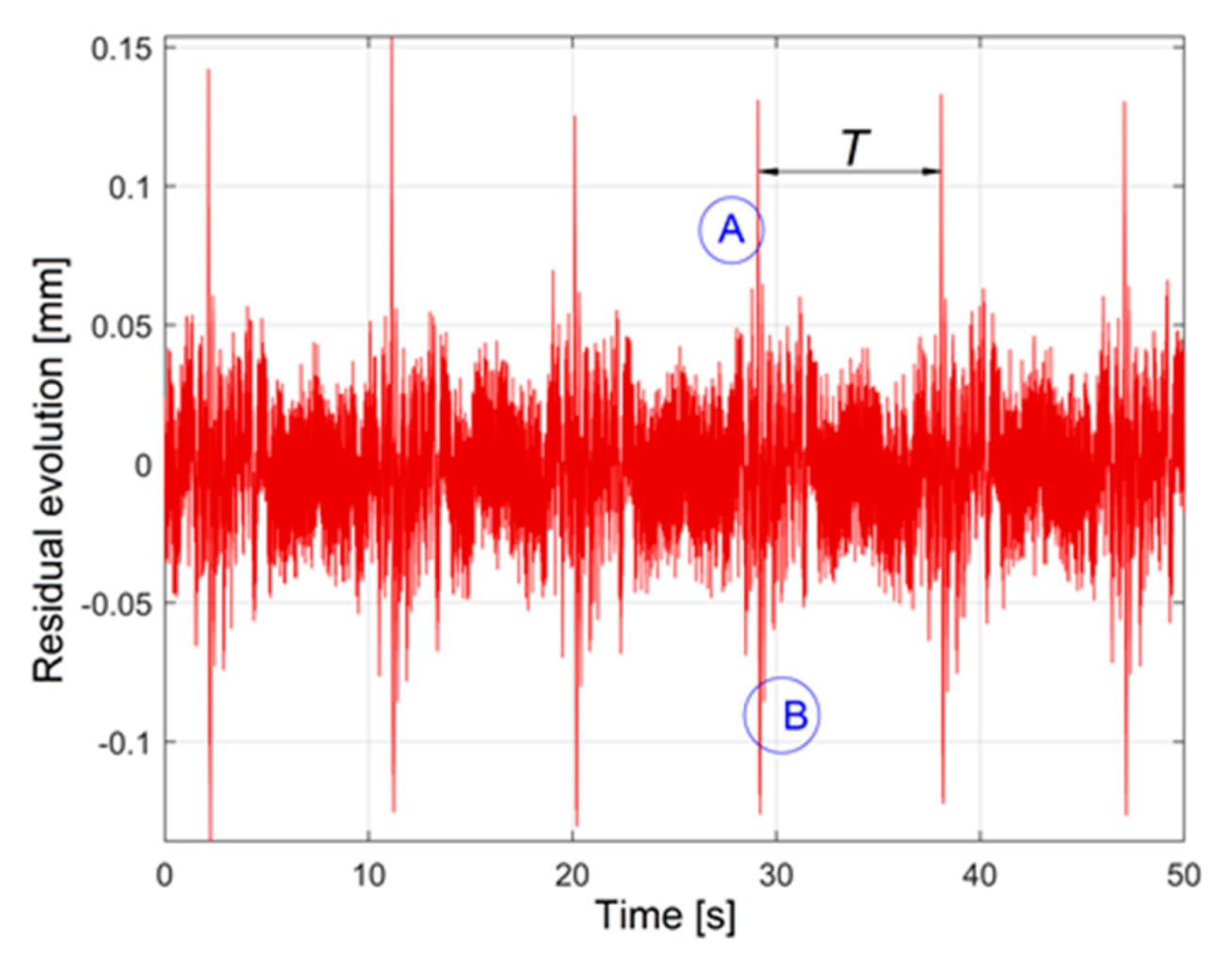
The evolution of residuals x_r(t) = x(t) − x_a(t) and y_r(t) = y(t) − y_a(t) from curve fitting of x and y-motions using a sine model are described in Figure 6 and Figure 7 (with the same scale). The shape and the magnitude of residuals proves that x and y-motions are not perfectly harmonic (as expected), as a new indicator for the lack of P&A of circular trajectories.

The evolution of residuals from Figure 6 and Figure 7 indicates that the negative effect on P&A of x-motion errors is smaller than of y-motion errors.

It is interesting to find out if there is a recurrent (or repeating)periodical pattern of the residual evolutions (x_r, y_r) on a complete period T of each motion (x, y). A simple way to check if there is a recurrent periodical pattern on x_r, and y_r evolutions is to build an average evolution of the residual (x_Ar, y_Ar) on a single period T with these definitions:

$$x_{Ar}\left(t\right)=\frac{1}{k}{\displaystyle \sum }_{i=0}^{k-1}{x}_r\left(t+i·T\right)y_{Ar}\left(t\right)=\frac{1}{k}{\displaystyle \sum }_{i=0}^{k-1}{y}_r\left(t+i·T\right)$$

(2)

Figure 8 presents the evolution of x_Ar(t = 0 ÷ T, with 179,740 samples) with k = 5 (for five completely circular trajectories), each sample of x_Ar being an average of k correlated samples of x_r. It is obvious that the x-motion has a well-defined repetitive periodical pattern, with systematic errors. In other words, x_r (and x-motion as well) is well correlated with itself.

The curve fitting of x_Ar evolution using a sum of sine model delivers the analytical evolution x_aAr of x_Ar as Figure 9 indicates. In Equation (3) is depicted the analytical model for x_aAr as it follows:

$$x_{aAr}\left(t\right)={\displaystyle \sum }_{j=1}^n{a}_{xj}·\sin \left(b_{xj}·t+c_{xj}\right)$$

(3)

With n = 16, the values of a_xj, b_xj and c_xj involved in x_aAr model from Equation (3) are depicted in

Table 1. The values of a_xj, b_xj and c_xj involved in x_aAr model from Equation (3) with n = 16.

j	axj[mm]	bxj[rad/s]	cxj[rad]	j	axj[mm]	bxj[rad/s]	cxj[rad]
1	0.203	0.3379	1.969	9	0.001888	6.191	−2.542
2	0.004801	4.885	0.3713	10	0.002353	119.3	1.698
3	0.004398	1.383	1.758	11	0.1188	121.8	2.263
4	0.003755	2.083	1.377	12	0.001696	44.14	−3.301
5	0.004055	4.163	−2.608	13	0.00148	120.4	−0.3449
6	0.004279	3.47	−2.578	14	−0.1166	121.8	2.283
7	0.1981	0.3481	−1.225	15	0.001224	123.3	−2.064
8	0.001892	42.6	−2.541	16	0.0004954	118.6	−2.431

(as results of x_Ar curve fitting).

A better model x_aAr for x_Ar is available by increasing the value of n. There is not a total fit between x_aAr and x_Ar, mainly because the model is not able to describe the phenomena characterized by temporary variations of amplitudes.

On this subject, Figure 10 presents a detail with x_aAr and x_Ar evolutions located in the area A of Figure 8 with n = 105 (105 components in sum of sine model from Equation (3)). The strong variation of displacement depicted here is likely the result of structural vibrations of the 3D printer induced by the stepper motor.

The x_Ar and x_aAr evolutions are certain arguments that the experimental setup is able to describe the P&A of x-motion. Moreover, the analytical model from Equation (3) and Table 1 helps (at least in theoretical terms) to compensate for the errors of x-motion.

Figure 11 presents the evolution of y_Ar with k = 5 (for five completely circular trajectories, each sample of y_Ar being an average of k correlated samples of y_r). As with x-motion, it is obvious that the y-motion also has a well-defined periodic recurrent pattern (the same period T as x_Ar), having systematic errors. In other words, y_r (and y-motion as well) is well correlated with itself. Unfortunately, it was not possible to find an acceptable analytical model y_aAr with harmonic components (similar to the x_aAr model for x_Ar based on Equation (3)). A very high number of harmonic components (n) is necessary in this sum of sine model. A future approach intends to identify a more appropriate analytical model. There are strong repetitive irregularities on y-motion (and y_r and y_Ar as well) revealed in A, B areas of Figure 8 and Figure 11. Likely they are irregularities generated by a suddenly releasing of a mechanical stress inside the toothed belt used to produce the y-motion.

It is interesting now to examine the average trajectory generated by the 3D printer with x_a(t) + x_Ar(t) = x_e(t) as x-motion and y_a(t) + y_Ar(t) = y_e(t) as y-motion. It is obvious that this trajectory is not a perfect circle (at least because the wrong phase shift between x_a and y_a). A computer program was developed in order to find out the description of the least square circle (the coordinates x_c, y_c of center and the radius R_c as well) by circular fitting. This program is available for the fitting of any closed curve with known analytical description. The circular fitting supposes to find out the values x_c, y_c and R_c for which a fitting criterion ε described in Equation (4) reaches a minimum value.

$$\epsilon ={\displaystyle \sum }_{i=1}^N\left[{\left(x_{ei}-x_c\right)}^2+{\left(y_{ei}-y_c\right)}^2-R_c^2\right]$$

(4)

In Equation (4), N is the number of samples x_ei or y_ei (N = 179,740) used for x_e-motion or y_e-motion description of the average trajectory. If the average trajectory is a perfect circle, then a perfect fitting produces a value ε = 0 for the fitting criterion. The circular fitting of average trajectory produces x_c = 0.00303 mm, y_c = 0.00252 mm and R_c = 8.9873 mm (this radius being very close to the amplitudes of x_a and y_a already revealed in Equation (1)). A first conventional graphical description of the circularity error of the average trajectory (as a first trajectory fitting residual, TFR₁) is available in polar coordinates (d_i1, α_i1), related to the least square circle, with d_i1, α_i1 defined as:

$$d_{i1}=\left|\sqrt{{\left(x_{ei}-x_c\right)}^2+{\left(y_{ei}-y_c\right)}^2}-R_c\right|{\alpha }_{i1}={\mathit{arctan}}^4\left(\frac{y_{ei}-y_c}{x_{ei}-x_c}\right)$$

(5)

Here d_i1 is the distance from average trajectory to the least square circle, α_i1 is the polar angle, with arctan⁴ the inverse of tangent function in four quadrants. This TFR₁ is also available in Cartesian coordinates as a curve described by a movable point having d_i1·cos(α_i1) + x_c as abscissa and d_i1·sin(α_i1) + y_c as ordinate. If the average trajectory is a perfect circle, then TFR₁ is a point placed in the center of the least square circle.

Figure 12 presents the TFR₁ of the average trajectory with a circular grid (with a 20 μm increment on radius). Here the maximum value of distance d_i1 is 145.8 μm.

It is interesting to explain why TFR₁ from Figure 12 has four almost similar lobes. The dominant component (as amplitude) in x_e-motion is x_a, while the dominant component in y_e-motion is y_a (with x_a and y_a experimentally revealed by fitting and depicted in Equation (1) as pure harmonic motions).

As previously shown, these two components (having the same amplitude and angular frequency) are not rigorously shifted with π/2 (as expected).This means that the dominant part of the average trajectory (generated by x_a and y_a motions composition) is not a circle (as expected) but an ellipse. 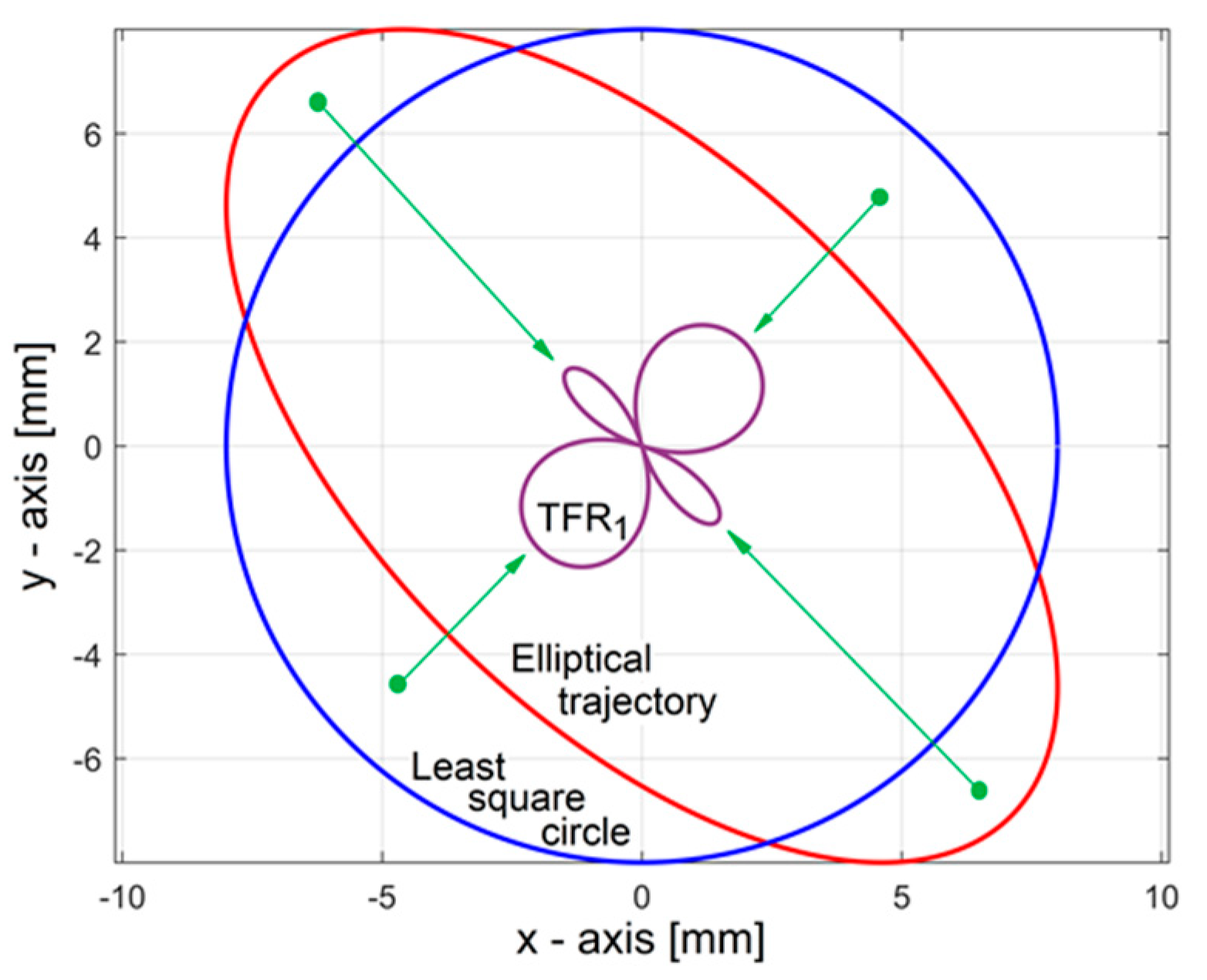The circular fitting of an ellipse produces a least square circle which intersects the ellipse in four points and a TFR₁ with four lobes, according to the simulation results from Figure 13 (with an elliptical trajectory generated by two harmonic signals shifted with 2.1863 radians). A better explanation for these four lobes in Figure 12 is produced if over this figure is added the TFR₁ of the trajectory generated only by x_a and y_a-motions, with green color, as Figure 14 indicates (here both curves being traversed counter clockwise). A better approach to the shape of TFR₁ involved in Figure 14 is produced if the distances d_i1 from Equation (5) are calculated related by a circle with smaller radius than the radius of the least square circle (R_c), as TFR_1a. As example, in TFR_1a from Figure 15, this radius is R_c − 0.025 μm.

For P&A evaluation of the average circular trajectory (the result of x_e and y_e simultaneous motions), an important item is the size of the surface delimited by the trajectories fitting residuals (TFR₁ and TFR_1a). Each area is a sum of the areas of N-1neighboring triangles. All triangles share a common vertex placed in the origin of coordinate systems. The other two vertices are two successive points on TFR. With the area formula of a triangle from [30] (based on the vertices coordinates), the total area delimited by TFR₁ generated by x_e and y_e (Figure 12 or Figure 14) is calculated as 8515.3 μm², while the total area delimited by TFR₁ generated by x_a and y_a (Figure 14) is 7624 μm².

A second conventional graphical description of the circularity error of the average trajectory (as a second trajectory fitting residual, TFR₂) is available in polar coordinates (d_i2, α_i2) related to the minimum circumscribed circle (having the same center as the center of the least square circle), with d_i2, α_i2 defined as:

$$d_{i2}=\sqrt{{\left(x_{ei}-x_c\right)}^2+{\left(y_{ei}-y_c\right)}^2}-R_{cc}{\alpha }_{i2}={\mathit{arctan}}^4\left(\frac{y_{ei}-y_c}{x_{ei}-x_c}\right)$$

(6)

In the first Equation from (6), $R_{cc}=\min \left(\sqrt{{\left(x_{ei}-x_c\right)}^2+{\left(y_{ei}-y_c\right)}^2}\right)$ is the radius of the minimum circumscribed circle.

Figure 16 presents the TFR₂ of the average trajectory generated by x_e and y_e (R_cc = 8.8434 mm) and TFR₂ generated by x_a and y_a (with green color, R_cc = 8.9171 mm), with circular grid (with a 50 μm increment on radius). Here the maximum value of distance d_i2 is 246 μm.

A TFR₂ for a perfect circular average trajectory is a point placed in the origin of the least square circle.

The existence of these two lobes on TFR₂ in Figure 16 is explicable if, in addition to the comments and simulation done in Figure 13, we take into account that the minimum circumscribed circle touches the elliptical trajectory in two symmetrical points. The TFR₂ evolution of a pure elliptical trajectory related to the minimum circumscribed circle is depicted in Figure 17 (by simulation).

Some supplementary resources on the P&A of circular trajectories are revealed by circular fitting of the 2D curve generated only by x_Ar-motion (already described in Figure 8) and y_Ar-motion (already described in Figure 11), as Figure 18 indicates.

The least square circle (14.2 μm radius, with center at x_c = −3.3 μm and y_c = −1.9 μm) should also be considered as an indicator for P&A of the average trajectory.

We should mention that the effect of strong repetitive irregularities on y-motion (y_r and y_Ar) already revealed in A, B areas on Figure 8 and Figure 11 are also well described in Figure 14, Figure 15 and Figure 16 and Figure 18. Moreover, the mirroring of these events A, B in Figure 14 or Figure 15 confirms the previously formulated hypothesis (the comments in Figure 11) that they are related by a sudden release of a mechanical stress inside the toothed belt used for y-motion. In Figure 11, a maximum positive peak from A is immediately followed by a minimum negative peak from B. Therefore, in Figure 14, these two peaks A, B are described as a single peak because of modulus in definition of d_i1 (Equation (5)).

As it is clearly indicated in Figure 8 and Figure 11, there are strong vibrations on both motions (on x and y), with a negative effect on the P&A of circular trajectories. There are two different strategies available to reduce or to eliminate these vibrations.

The first strategy (probably as the better approach) is to use each stepper motor also as an actuator inside an open-loop active vibration suppression system. The second strategy is to use passive dynamic vibration absorbers or tune mass dampers as well [31] placed on the print bed and on the extruder system. The effect of vibration suppression on TFR₁ or TFR_1a shapes should be similar to the effect of a low pass numerical filtering of x_e and y_e. Figure 19 presents the new shape of TFR_1a (as TFR_1af) if x_e and y_e motions are filtered with a moving average numerical filter (with 1000 samples in the average). As expected, the size of the surface delimited by the TFR_1af is not significantly changed (17,399 μm² here by comparison with 17,711 μm² on TFR_1a from Figure 15). The evolution of TFR_1af from Figure 19 is also useful when only the influence of the low frequency variable components from x_e and y_e-motions on P&A is investigated and used for errors compensation. The compensation is a feasible option with an appropriate control of stepper motors since they are operated using the microstepping drive technique [32].

If the accuracy describes how close the real trajectory is to a desired circle (or how close the shapes of TFR₁, TFR_1a and TFR_1af by a point are), the precision describes the repeatability of real trajectories, each trajectory being generated using a complete cycle (period) of x and y-motions, partially described in Figure 4. The best way to compare these real trajectories is to use the comparison between trajectories fitting residuals related to a circle with a smaller radius than the radius of least square circle (defined similarly to TFR_1a) but using low pass filtered x and y-motions (as TFR_3af). A perfect coincidence of real trajectories should produce a perfect coincidence of TFR_3af trajectories. 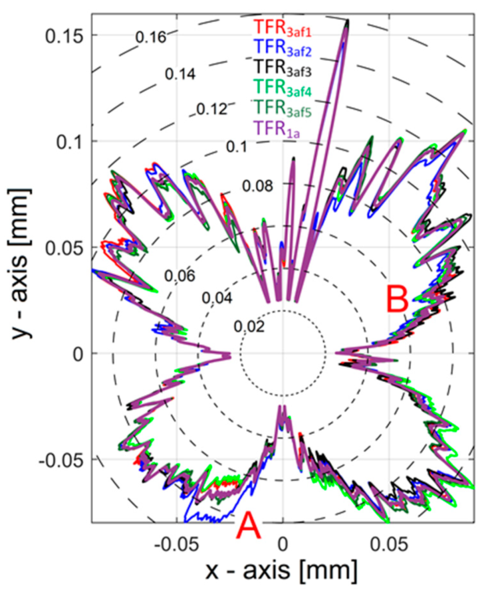Figure 20 presents the evolution of TFR_3af for five successive real trajectories (TFR_3af1 ÷ TFR_3af5) and the evolution of TFR_1a.

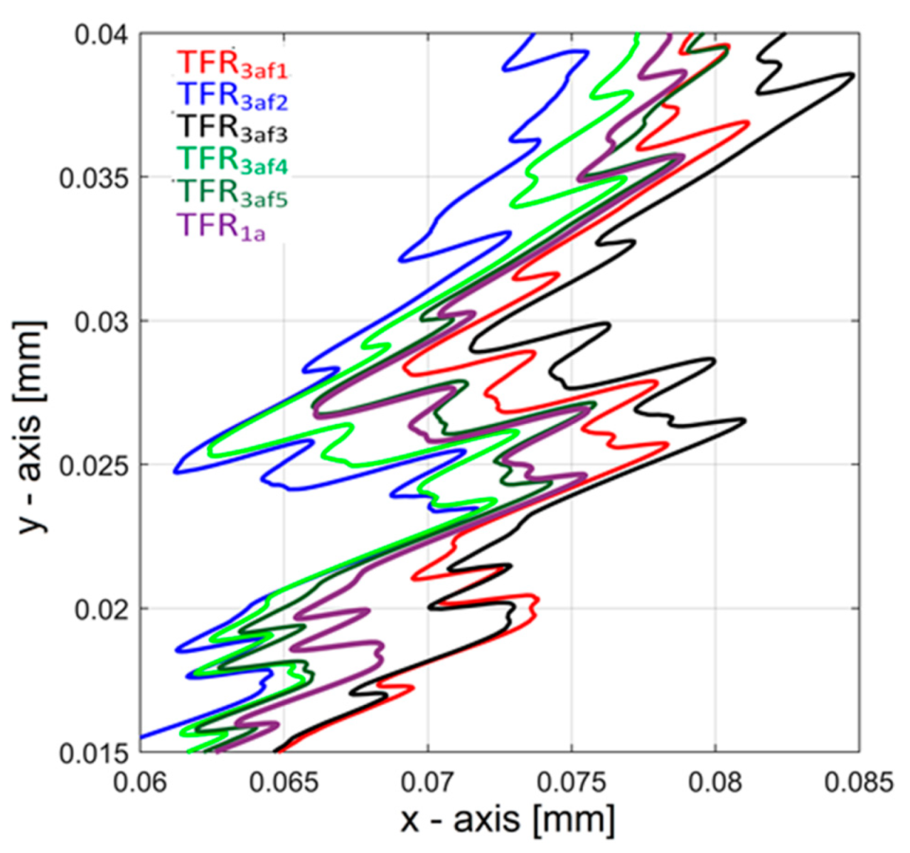
Figure 21 presents a zoomed in detail of Figure 20 in area B. As expected, there is not a perfect coincidence of TFR_3af trajectories, despite some certain shape similarities (except in area A on Figure 20 where the trajectory TFR_3af2 is extremely different). It is obvious that the difference between trajectories is less than 10 μm (except in area A). Without any improvement of the 3D printer structure and kinematics, this should also be the theoretical precision after an eventual compensation of the errors (using an appropriate control of the stepper motors). With ideal errors compensations, the trajectories TFR_1f should be bordered outside by a circle with 10 μm radius (or 35 μm radius for the trajectories TFR_3af).

A complete estimation of 3D printer P&A should consider specific trajectories (e.g., circles as in this study) placed in different positions in different 2D locations of the printing volume travelled with different speeds, clockwise and counter clockwise.

4. Conclusions and Future Work

Some theoretical and experimental approaches related to the precision and accuracy (P&A) of a 3D printer, particularly for 2D circular trajectories, were achieved in this paper. The choosing of 2D circular trajectories was inspired from ISO standards methods for P&A evaluation of CNC manufacturing systems (ISO 230-4 [27]) due to some similarities in terms of motion control. The evolution of the simultaneous displacement on two theoretically orthogonal axes (x and y) during a repetitive 2D circular trajectory of the extruder system related to the print bed was simultaneously and continuously measured using a computer-assisted setup based with two contactless optical sensors and a numerical oscilloscope (for sampling and data acquisition). The signals of description for x and y-motions were numerically processed in order to find out some motions characteristics involved in the evaluation of P&A for circular trajectories.

First, a non-perpendicularity of x and y-axes (or an axis misalignment) were experimentally detected (with 0.893 degrees error) by means of the curve fitting (using a pure sine model) of the dominant harmonic components of each signal (x and y-motions signal). Because of this error, a circular programmed trajectory is executed as an elliptical one (typically for a non-orthogonal x0y coordinate system), a topic also confirmed by some supplementary signal processing results.

Second, it was established that the x and y-motions are not simple pure harmonic motions. The residuals of previous curve fitting on each axis movement describe the deviation from pure harmonic shape. A procedure for finding a repetitive periodical pattern in the evolution of these residuals was established and applied with good results. The model of each repetitive pattern is useful in the amelioration of P&A by correction and compensation. The analytical description of the x-motion residual pattern was already established (by curve fitting with a sum of sine model); a future approach intends to do the same for y-motion residual.

Third, a procedure of the description for an average 2D trajectory (an average of several successive theoretically identical circular trajectories) was established. A computer-aided procedure of fitting for closed curves (particularly a circular trajectory) was developed. The circular fitting of the 2D average trajectory was done related to the least square circle. Two conventional graphical descriptions of the circularity errors of the average trajectory were proposed (as trajectory fitting residuals TFR₁ and TFR₂): first description being related to the least square circle, second related to the minimum circumscribed circle.

The shape of these trajectories fitting residuals and the size of the surface delimited by them are useful in P&A evaluation of circular trajectories in order to verify that the 3D printer works properly and, especially, for systematic errors compensation purposes. For example, the non-perpendicularity of x and y-axes previously detected is mirrored in the shape of the average trajectory and, finally, in the shape of these two trajectory fitting residuals (with four similar lobes on TFR₁ and two similar lobes on TFR₂). The deviation from the harmonic shape for x and y-motions is described on these trajectories.

A future approach will be focused on finding a complete procedure of experimental research of P&A using high range/resolution non-contact displacement sensors placed on each of three axes. Some complex 3D curves will be used as test trajectories. A numerical interface between the experimental setup and the 3D printer will be developed in order to perform automated testing and errors compensation.

These signal processing procedures are available to verify the P&A of 2Dcircular trajectories on any other similar equipment (e.g., a 3D CNC manufacturing system).