Article

Interferometric Satellite Data in Structural Health Monitoring: An Application to the Effects of the Construction of a Subway Line in the Urban Area of Rome

1
Department of Mechanical and Aerospace Engineering, Politecnico di Torino, 10129 Turin, Italy
2
Department of Structural, Geotechnical and Building Engineering, Politecnico di Torino, 10129 Turin, Italy
*
Author to whom correspondence should be addressed.
Submission received: 30 December 2021 / Revised: 26 January 2022 / Accepted: 27 January 2022 / Published: 5 February 2022
(This article belongs to the Special Issue Novel Approaches for Structural Health Monitoring II)

Abstract

:
In recent years, the use of interferometric satellite data for Structural Health Monitoring has experienced a strong development. The urban environment confirms its fragility to adverse natural events, made even more severe by climate change. Hence, the need to carry out continuous monitoring of structures and artefacts appears increasingly urgent. Furthermore, satellite data could considerably increase the feasibility of traditional Structural Health Monitoring (SHM) approaches. This study aims to explore this remote sensing approach, focusing on the representation techniques that can be adopted to highlight their advantages and provide an interpretation of the results. In particular, the study analyzes records from the urban area of Rome (Italy), subject to the construction of a new subway line. These data are exploited to create a velocity map to highlight the possible subsidence phenomenon induced by excavations. Then, the paper focuses on single buildings or building complexes through the entropy-energy representation. Beyond the different limitations caused by the input data, a correlation is identified between the results of the two representation techniques. Accordingly, the effects of excavation on the urban area are demonstrated, and the methodologies are validated.

1. Introduction

In recent years, the built environment and entire urban areas have been subjected to many adverse natural phenomena or extreme events, which can often be linked to advancing climate change. It highlighted how buildings, infrastructures and architectural heritage structures are highly fragile and vulnerable. Therefore, there is a growing concern in approaches to examine the built environment and, in particular, the constructions with strategic or historical/architectural value to ensure higher safety and reliability or predict the structural behavior in case of unforeseen events. Thus arises the need for novel Structural Health Monitoring (SHM) techniques and technologies capable of providing continuous datasets, with high efficiency and reduced costs.
Indeed, traditional SHM applications require the use of a high number of sensors (e.g., accelerometers for motion measuring, thermocouples, anemometers, etc.) [1], which can prove costly. Among new SHM technologies, the possibility of using remote sensing techniques [2], especially data gathered by constellations of artificial satellites, is becoming a viable option. Satellites allow observing the earth’s surface through the interaction of electromagnetic waves, with objects placed even at a considerable distance from the observer [3]. The main advantages are to guarantee a broad coverage both spatially and temporally, with a low environmental impact.
The potentialities of applying satellite remote sensing for urban applications have been highlighted as long ago as in 1985 by Foster [4]. However, the employment of this remote sensing approach for civil SHM is recent and has been fostered by the increase in data quality and the development of new algorithms for data processing.
The satellite sensors use radar waves, characterized by wavelengths in the range between 1 m and 1 mm. In addition, data can be acquired regardless of the presence of sunlight and can be used even in sub-optimal weather conditions (e.g., in the presence of clouds). Satellites commonly roughly follow polar orbits, with a slight inclination angle to the meridians, and descending and ascending orbits are distinguished depending on the pole toward which the satellite moves. The direction along which there is the emission and reception of the signal is called Line of Sight (LOS) and is the direction along which the sensors gather the images and information about the displacements of points on the earth’s surface.
The new SHM approaches exploit the radar images gathered from satellite constellations, adopting Synthetic Aperture Radar (SAR). It is a satellite radar acquisition technique that uses the synthesis of a virtual antenna with a kilometric aperture to improve spatial resolution. This virtual antenna is simulated by acquisitions made on the same area, observed at different times and positions by the same satellite [5].
Among SAR acquisition techniques, the Interferometric SAR (InSAR) is employed to extract displacement information. It allows describing interferograms by comparing the SAR data over a baseline time and evaluating the differences between the measures [6]. A particular kind of InSAR is the Differential Interferometry SAR (DInSAR), in which only the pure displacement components of the differential satellite target phases are depicted from the images acquired by the satellite in the same area at different time instants.
Satellite interferometric data have already been exploited in some early SHM applications for urban areas and to quantify large-scale phenomena, such as land subsidence [7,8,9,10,11,12]. Recently, the need for efficient real-time monitoring of damage led to the development of new techniques, such as the multi-temporal InSAR (MT-InSAR) [13]. By combining different differential interferograms, MT-InSAR approaches more accurately provide the trends of displacements in the area of interest and their temporal evolution. Therefore, they have been applied to detect anomalies in a single structure [14] and for the assessment of tunnel-induced subsidence and related damage [15]. Despite the advantages afforded by this new approach, there are still many limitations and challenges to overcome [16,17]. They are mainly due to the differences between satellite data and the information required by traditional SHM techniques and obtained from in situ sensors.
Furthermore, new visualization/representation approaches are necessary to give a relevant interpretation of the measures provided by satellite datasets. This issue is of primary importance to realize automatic procedures for the assessment of structures’ behavior and for the diagnosis of anomalies, which may be connected to structural damage. The main representation techniques refer to the distribution of direct quantities (i.e., displacements along the LOS, velocities along the LOS). However, it is also possible to create maps or diagrams of indirect measures to enhance data interpretation. It is the case of spectral entropy-energy graphs, which can be used to estimate the average information of the signal and to characterize the behavior of a system.
This study aims to explore and compare the possibilities given by the different methodologies of satellite data representation and to highlight the advantages provided by the evaluation of spectral entropy for the description of whole structural systems. This is accomplished by analyzing the case study of the area of Rome (Italy) subject to excavations for the construction of the T3 section of the subway line C. This work is under construction, which began in 2013, and affects an area rich in architectural heritage.
This paper is organized as follows: Section 2 briefly describes the characteristics of the satellite data employed and the proposed representation approaches; Section 3 concerns the results of the case studies; finally, conclusions are presented in Section 4. The case study initially focuses on representing data at a territorial scale to identify the subsidence phenomena induced by the excavation of the two tunnels of the underground railways. Then, the entropy-energy diagram is adopted to describe single monumental buildings or building complexes, highlighting the presence of points with outlier signals. However, the data used for this representation refer to a period that is insufficient to detect an actual anomaly in the structural behavior due to the poor frequency content. Consequently, the two types of representation used are compared to verify the results and obtain cross-validation of the methodology. A further comparison is made between the representations in the first and second parts of the analyzed period for a small complex of structures, as well as for the monumental Colosseum structure.

2. Materials and Methods

The analysis conducted employs the ascendant SAR images acquired by the COSMO SkyMed (CSK) satellite constellation in the period from March 2011 to March 2019, the same data employed in the DPC-ReLUIS 2019–2021 project [18]. CSK is an earth observation mission conceived for civil and military purposes, developed by the Italian Space Agency (ASI) [19] in cooperation with the Ministry of Defense. It is based on a constellation of low earth orbit satellites equipped with SAR working in X-band. The differential interferometric SAR information is processed by adopting the Small Baseline Subset algorithm (SBAS–DinSAR) [20,21]; thus, it is possible to obtain the displacements with the accuracy of centimeters and millimeters.

2.1. Satellite Data

It is necessary to underline that the satellite data used are subjected to different levels of preliminary treatments to obtain SAR standard products and higher-level products, such as the interferometric ones [22,23]. Afterward, these are additionally processed according to the SBAS–DinSAR algorithm [20,21]. The processing methods could cause new difficulties in the further treatment of data, e.g., the improper elimination of useful points, or the preservation of non-structural points, increasing the uncertainty of the results [16]. In addition, it has to be considered that the LOS data do not refer to the point on the ground, but to the point measured by the sensor (e.g., the roof of a building). Thus, to exploit them in the assessment of subsidence, the simplifying assumption of having structures undergoing a uniform subsidence phenomenon is introduced. Finally, a further limitation in the use of satellite data is due to the presence of a large dataset, in which points with incorrect measurements due to preliminary processing or insignificant ones (i.e., those that do not fall within the built area) are also included. As mentioned in reference [16], this presence contributes to increasing the analysis’ uncertainty, so these measures should be removed. However, this study considers an average, approximate behavior of the urbanized area and not the individual building. Therefore, this issue is neglected. For the evaluation of the case study, SAR images were extrapolated only for the area related to the T3 section of the Line C subway in Rome (Figure 1). This route connects the station of San Giovanni to the Colosseum, with an intermediate station (Amba Aradam/Ipponio). The area has great importance because it includes many structures of architectural and monumental value, such as the Colosseum itself, the Basilica of Santo Stefano Rotondo, the Basilica of Maxentius, the Aurelian Walls, the Colonnades of the Forum of Nerva and the Church of Santa Maria in Domnica. Although construction operations started in 2013, the project required various preparatory works and was subjected to delays. Therefore, tunnel excavation only began in 2018, after the inter-tract shafts realization in 2017 [24] (see Figure 1 for reference). This information is relevant for the identification of the area affected by the subsidence phenomenon induced by the excavations.
Regarding the soil characteristics, starting from the ground level, the stratigraphic succession shows the first layer of recent deposits, whose thickness reaches values of 13–16 m. It follows a layer of recent alluvial deposits lying on Pleistocene deposits, characterized in the upper portion by clayey silts and silty clays, locally sandy, and in the lower portion by sands and gravels. The water table level is placed at about 8–10 m from ground level. The depth of the tunnels is approximately 30 m between the San Giovanni and Amba Aradam stations, then increasing up to 57 m at shaft 3.2 and subsequently decreasing to 32 m at the Fori Imperiali station.
For each of the measured points, the employed dataset contains the geographic coordinates, the topographic elevation, the velocity and the LOS displacement at each time interval with respect to the initial one. The displacement and velocity values are given along the line of sight of the satellite sensor. Therefore, information on their overall deformation process can only be derived by processing the data obtained from both orbits (ascending and descending). However, a single dataset can still be used to obtain some preliminary information. In the case of subsidence phenomena, it can be assumed that the main direction of deformation is vertical. Thus, it is possible to derive the intensity of the displacement or the velocity along this direction, starting from the projection measured along the LOS of the satellite [18].
Furthermore, from a qualitative point of view, it is possible to observe only the displacements along the LOS, since, according to the assumption made earlier, a negative displacement or velocity (i.e., moving away from the satellite) is representative of a subsidence effect. From these presumptions, an interest in the representations/visualizations of direct quantities along the LOS arises. Furthermore, it is possible to derive valuable information from indirect measures, such as the spectral entropy of the signal.

2.2. Entropy Measures

According to Shannon’s definition, which is based on the concepts of information theory (IT), spectral entropy is a measure of uncertainty (or variability) associated with random variables [25]. It describes the information carried by a signal and allows quantifying its complexity. The introduction of this quantity for Structural Health Monitoring purposes arises from the assumption that the complexity of a structural system increases with the development of damage [26]. In the case of perturbations with specific, non-random behavior, there are low values of spectral entropy. On the contrary, a more complex and stochastic behavior leads to higher values of spectral entropy.
Shannon Spectral Entropy (SSE) evaluates the spectral power distribution from the Fourier transform of the signal to represent the dataset behavior in the whole observation period. Yet, it could be possible to use a spectrogram to estimate the instantaneous entropy and obtain its time series vectors. This study adopts the non-instantaneous spectral entropy, which is evaluated for each point of a system to describe the whole signal. In addition, the values are normalized with respect to the spectral entropy of the corresponding white noise to fit the regression inequalities rules. Given the signal x ( t ) , and the probability distribution P f in the frequency domain, the normalized Shannon Spectral Entropy is given by
H n = f = 1 N P f l o g 2 [ P f ] l o g 2 N
where N is the total number of frequencies, and l o g 2 N is the maximal spectral entropy of white noise. Consequently, this indirect measure can be used to realize maps or diagrams. In the following section, the spectral entropy is plotted on a dispersion diagram as a function of the signal energy. A regression model is adopted to highlight the trend and define the related probability distribution, which is used to impose a threshold for identifying the outliers.
The entropy-energy dispersion and the LOS information are evaluated together, employing scatter plots to assess how the points subjected to subsidence are located on the dispersion. In addition, the representations are evaluated for two subsequent periods, before and after the excavation, comparing their regression parameters to highlight the differences in the results.

3. Results

The present section describes the application of the interferometric satellite data to identify subsidence effects due to the excavation of the T3 section of Line C subway in Rome’s urban center. Firstly, the assessment is performed on a territorial scale of observation. Secondly, the entropy-energy representation is adopted to focus on the effects on a single structural system and to detect points with anomalous signals. In the third part, a comparison is discussed and, finally, the approach is applied to the Colosseum case study.

3.1. Territorial Scale Analysis

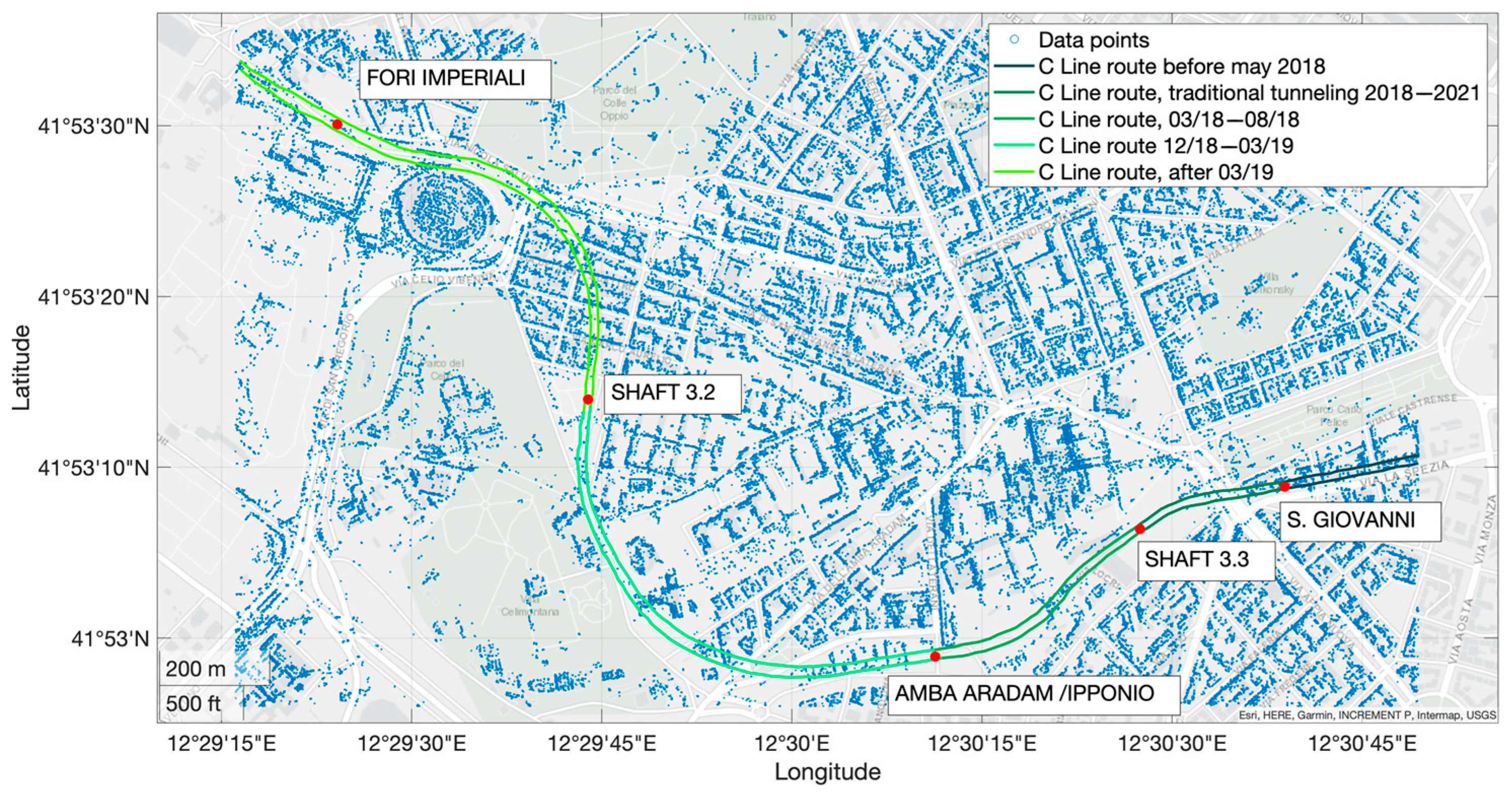
The subsidence effects induced by the excavation of the two subway tunnels can be observed in the years since 2017. In this period, the construction of the first section began with excavation performed using two TMB excavators. However, the entire route of the T3 section cannot be studied because it had not been finished by March 2019, which is the last time for which data are available. In detail, within this period, the excavations concerned the route from the station of San Giovanni to shaft 3.2, located in an intermediate position between the Amba Aradam/Ipponio station and the Colosseum, as shown in Figure 2. As a result, the area in which the displacements can be analyzed is further reduced.
The dataset contains the displacements along the LOS, which are used to evaluate the average annual velocity along the LOS. 
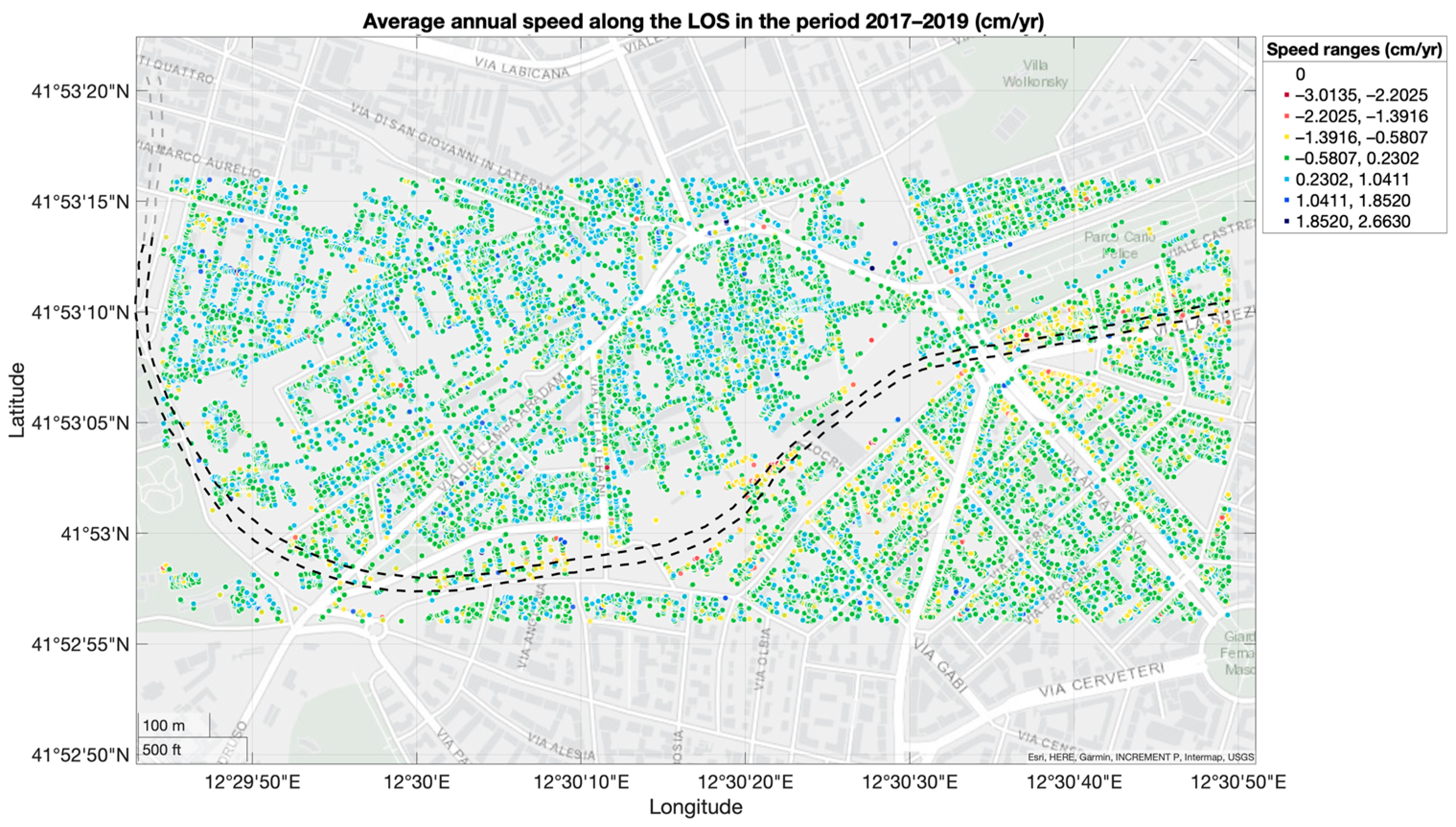
Figure 3 reports the velocity (cm/yr) on the map in the period from 2017 to 2019, while 
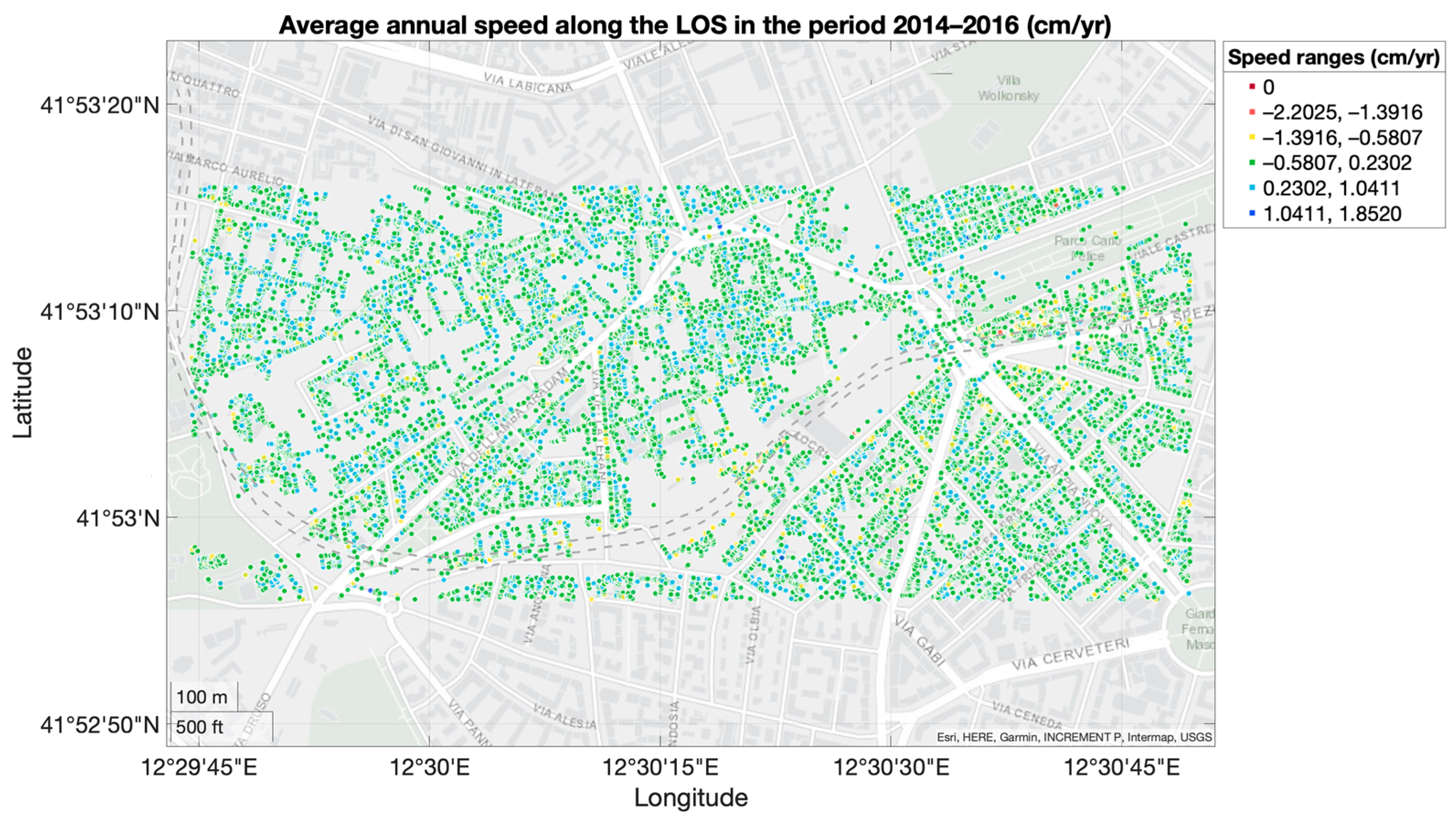
Figure 4 refers to the period from 2014 to 2016 and is used for comparison. It is worth observing that, in the period of the excavation (Figure 3), the velocity distribution presents a higher number of points with negative measures when compared to the previous years (Figure 4). These points are shown in yellow or red, and the negative value indicates that they are moving away from the satellite orbit, so they are qualitatively correlated to the subsidence phenomenon. As shown by the presence of negative values in Figure 4, it is not possible to exclude the possibility that subsidence also occurred before the construction of the metro line, for reasons uncorrelated with the excavations. However, it can be noticed how the points with negative velocity values strongly cluster along the subway route in Figure 3. Moreover, the underground work proceeded from the east of the reported area, moving westward; this may explain the larger concentration of these points on the rightmost portion of the figure.
To quantitatively study the subsidence phenomenon in the period from 2017 to 2019, the probability distribution of velocity values is estimated. Assuming a Gaussian distribution, the values have a mean equal to μ = 0.0440   cm / yr and a standard deviation equal to σ = 0.4132   cm / yr . This distribution allows identifying the negative outliers, points that deviate most from the general behavior of the distribution on the negative branch, in which the velocity is lower than μ 3 σ , that is to say, all the points with less than 0.14% probability of belonging to the same statistical distribution. From a physical point of view, these outliers can be interpreted as locations where subsidence is particularly prominent.
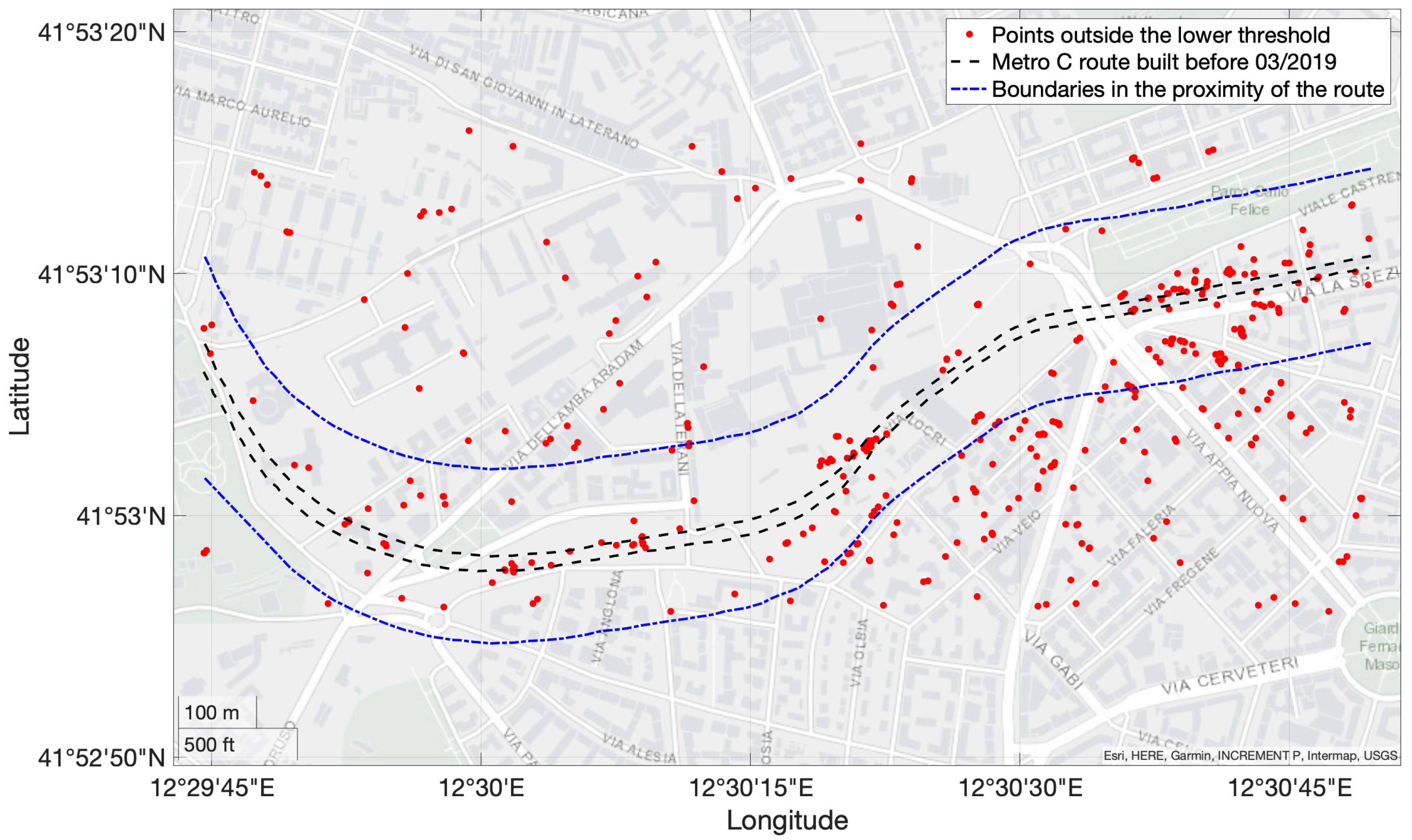
As seen in Figure 5, although the points outside this lower threshold are not exclusively distributed along the track, approximately 52% of them are concentrated in the route proximity (route ± 150 m). These points fall mainly on the route between San Giovanni station and the intermediate station of Amba Aradam/Ipponio, where the depth of the tunnels is about 30 m. On the other hand, in the latter part, the depth increases up to 57 m at shaft 3.2. Moreover, this portion of the track has been subjected to excavations near the end of the period for which data are available, so it was expected to find fewer points outside the threshold. The presence of excavation-induced subsidence was also confirmed in other studies [28,29].

3.2. Entropy-Energy Representation

The representations of mean velocity and entropy-energy data are basically complementary, that is, they provide different information, which are correlated. The entropy of a signal coming from a structural system defines its propensity to follow a deterministic behavior. That is to say, a lower entropy corresponds to a higher deterministic behavior. An output signal can change its characteristics due to: (i) system properties changes, and (ii) variation of input source. The interest here is only to input independent features; thus, what matters is how the entropy changes in relation to its energy value. This allows for discarding input-related variations, which are not of interest for SHM. When the entropy changes its value (in relation to its energy level) this means that the system changes its internal correlation (since entropy is used to estimate system complexity). Importantly, this can also happen if the mean velocities of the points remain constant; however, the opposite is not true, since an increase in the mean velocity would lead to higher energy and thus lower entropy. Thus, the mean velocity cannot change if the entropy-energy level remains constant.
Therefore, the energy-entropy representation implicitly carries more information than the mean velocity. The mean velocity is only representative of the displacement trend over time. Instead, any variation in the trend, frequency content, amplitude and phase is reflected in the entropy-energy representation.
An example is when a signal with zero mean increases its amplitude (e.g., due to a loss of stiffness). In this case, the mean velocity, being unchanged, would not allow for any novelty (thus, damage) detection. On the contrary, an increase in amplitude with constant mean velocity would lead to a change in entropy-energy values, and thus to a potential change of the complexity of the system. The mean velocity, however, is still an important datum to monitor because its straightforward physical meaning is connected to the rate of displacement in time (e.g., subsidence or swelling of the soil).
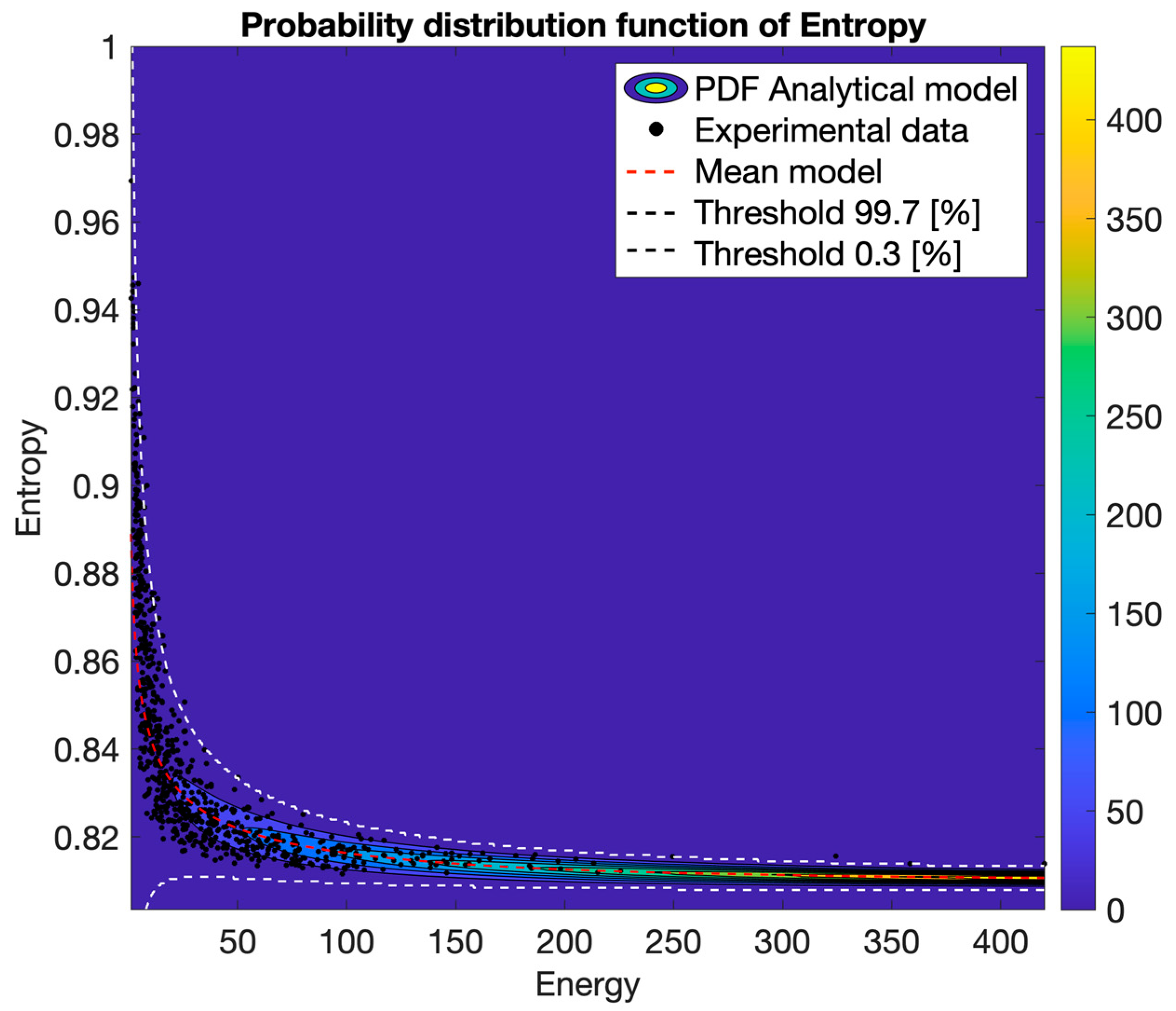
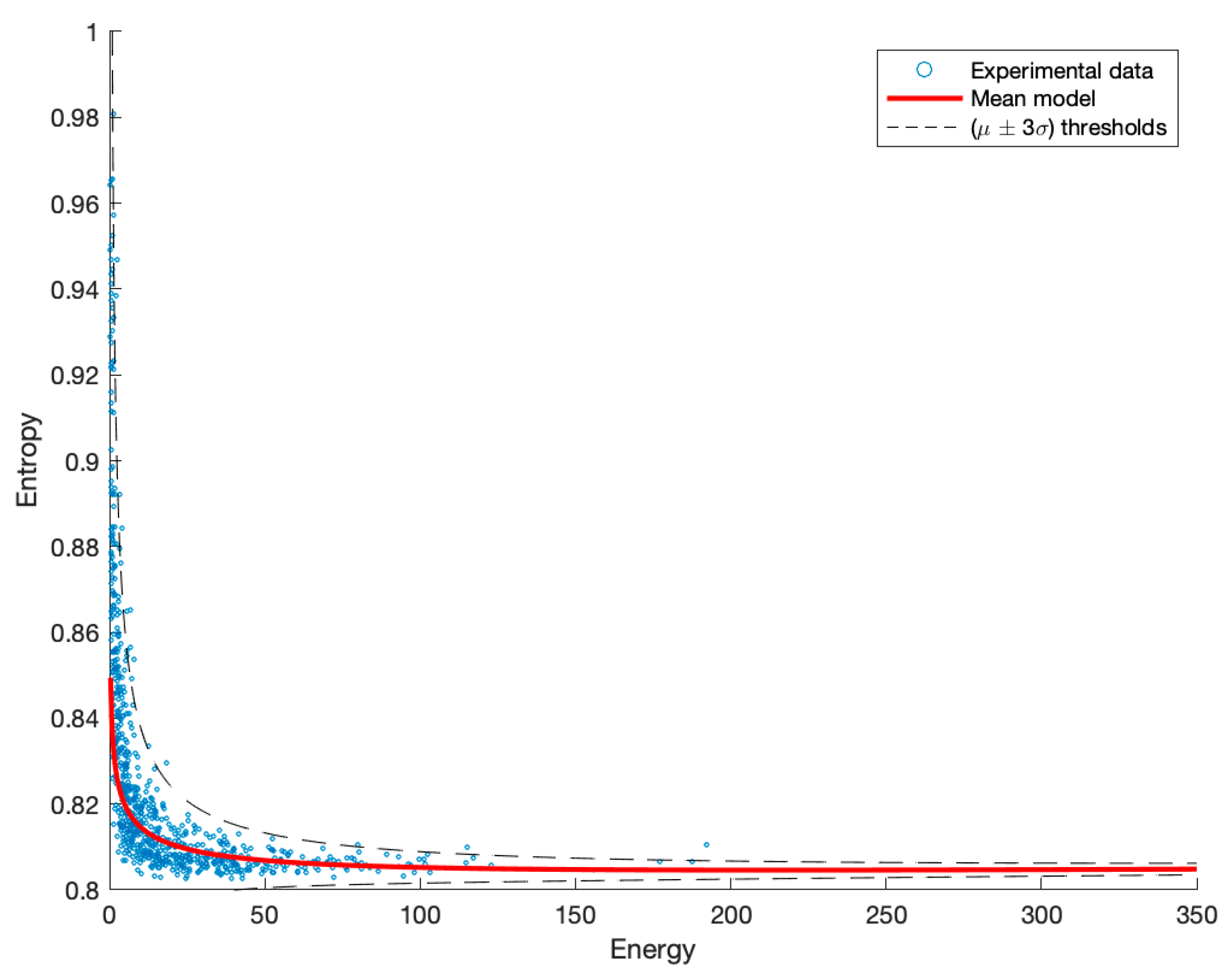
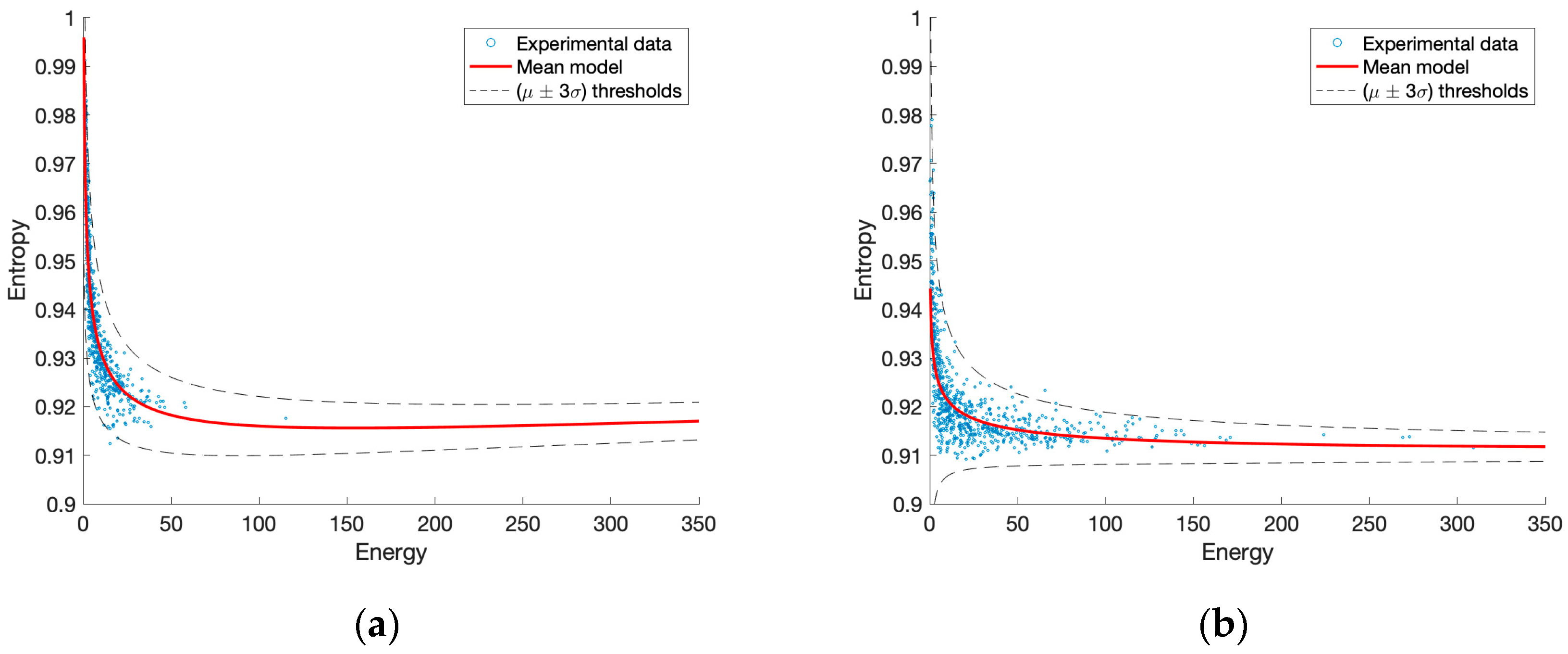
While it is true that entropy-energy representations cannot be adopted for the description of a whole urban area if the systems falling in the area are too different from a structural point of view, in the paper, the entropy-energy representation is used to study individual buildings. From the point scatter regression and probability distribution, it was possible to derive the limit curves (threshold 0.3% and 99.7%, according to the 3-sigma rule) and use them for the identification of outliers, i.e., points at which the signal deviates from the global analytical model and therefore requires further investigation. In order to quantify this deviation, the use of the Mahalanobis distance has been adopted. The points at which the entropy displays a low distance from the mean model can be interpreted as less stochastic (more deterministic). Conversely, if the entropy has a higher distance from the model, it indicates a less deterministic point.
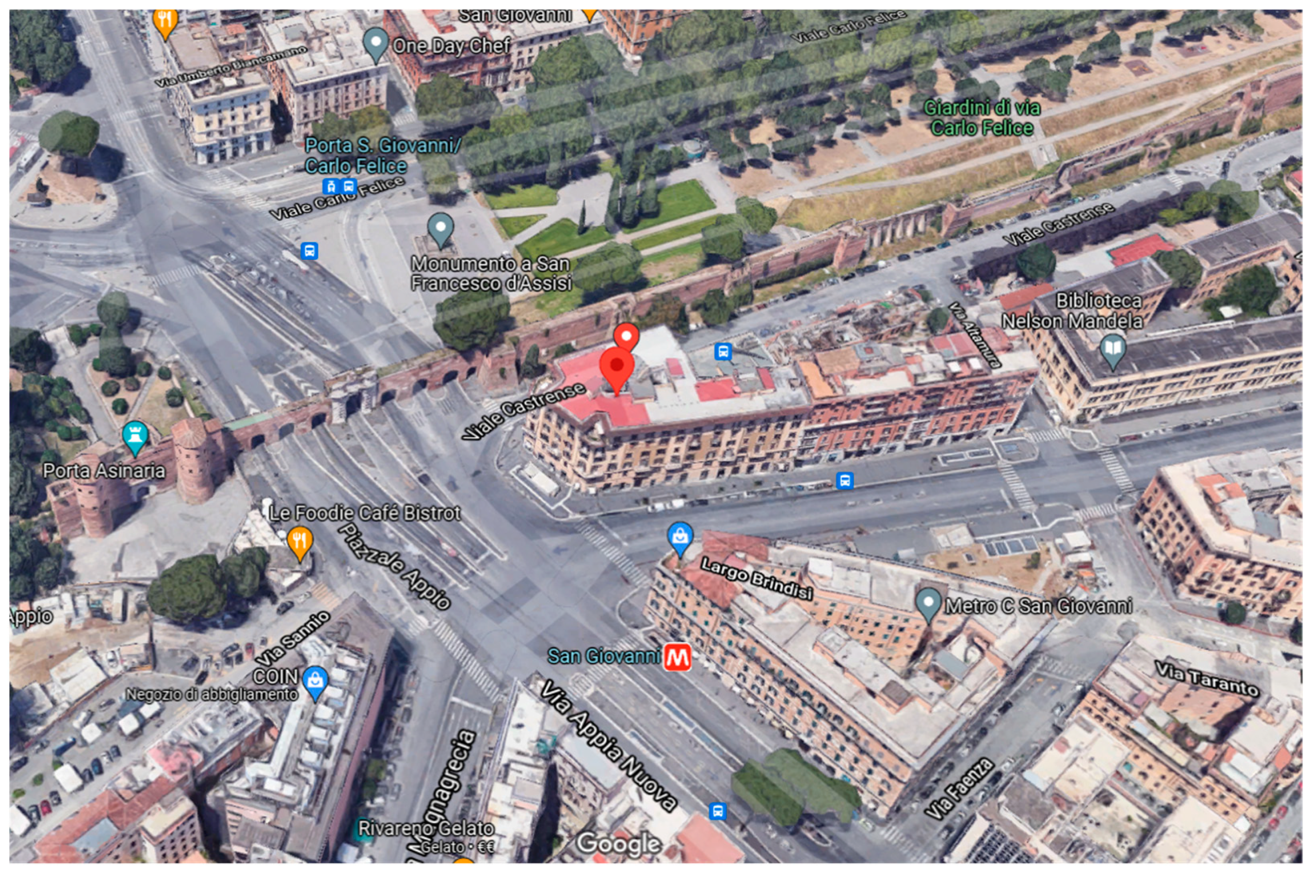
The following results refer to the building complex at the intersection of Via Emanuele Filiberto and Via Castrense (Figure 6), adjacent to San Giovanni’s station, in the period from 2017 to 2019. It has been analyzed as, according to the velocity, this area presents a concentration of points that are outside the subsidence threshold shown in Figure 5.
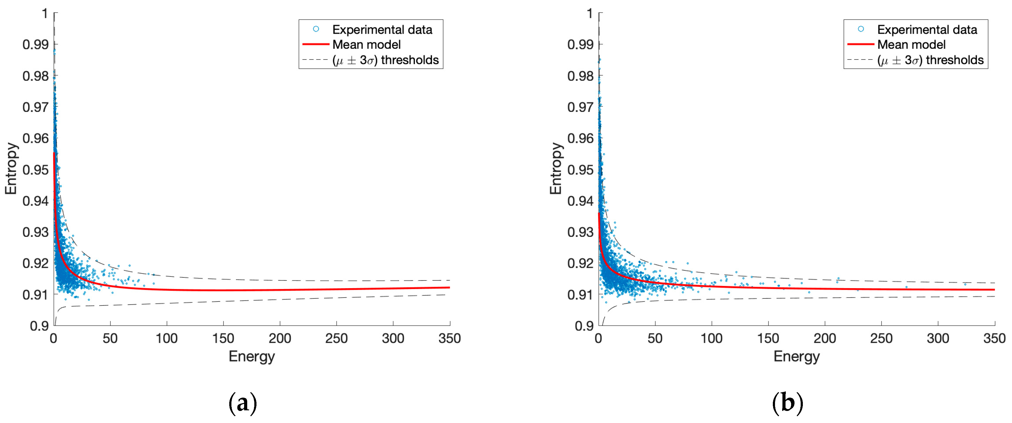
Figure 7 shows the dispersion of points and the mean model, which has a quadratic trend on a logarithmic scale. It also shows the analytical model’s probability distribution function (PDF) and allows the evaluation of the outliers.

3.3. Comparison of the Two Representations

The two approaches for representing the data shown above allow the localization of points of significant interest for monitoring structures and the subsidence phenomenon. These outcomes cannot be directly interpreted to perform novelty detection due to the limitations of the input data. However, it is possible to compare the results obtained through the two approaches to verify them. In detail, it is investigated how the points with a high-intensity negative velocity are distributed with respect to the values of entropy and energy of the signal. 
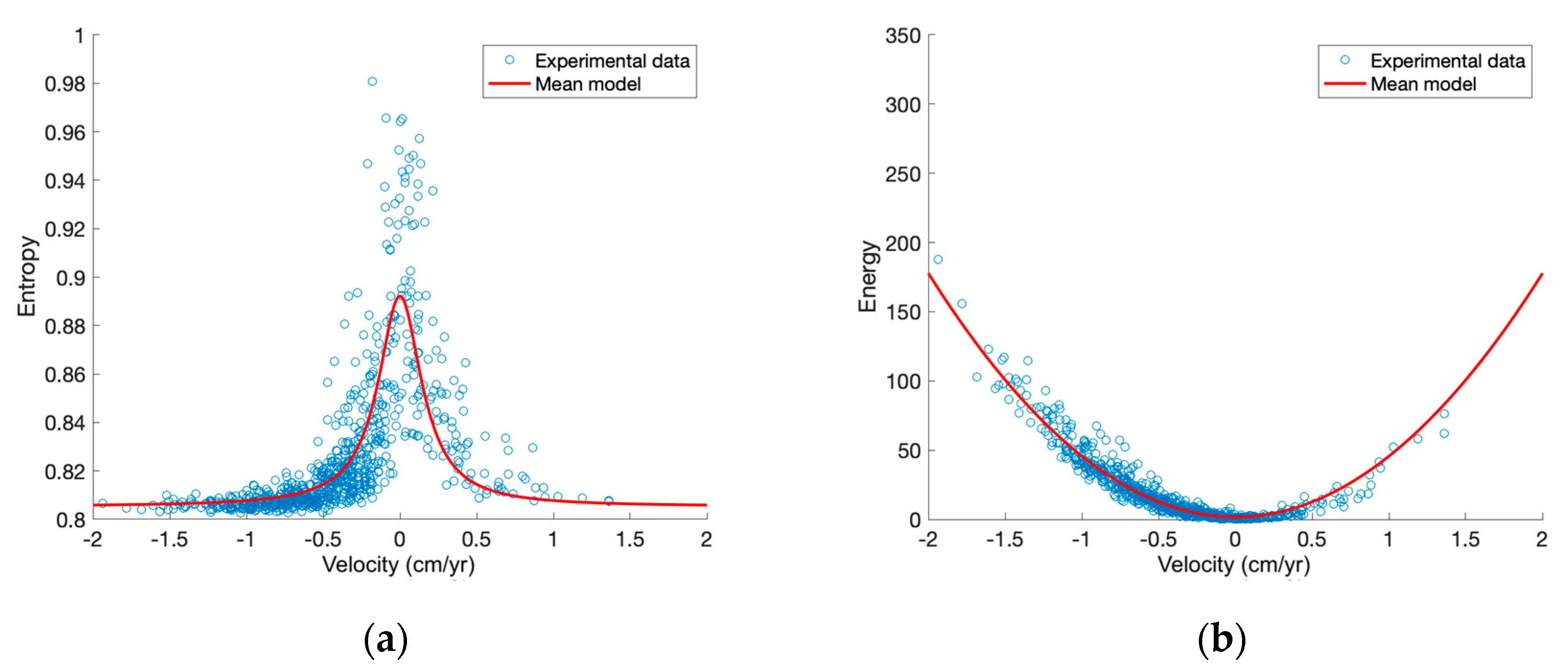
Figure 8a shows that points with higher absolute velocity have lower entropy values, concentrated in the range 0.8–0.82.
In contrast, points with velocities close to zero exhibit greater entropy. As the velocity increases beyond 0.5 cm/y, a further decrease in entropy is shown. Figure 8b shows how the energy remains low for velocity values close to zero and increases significantly for lower velocity values. These points correspond to locations subject to accentuated subsidence (beyond the μ 3 σ limit). Hence, in the entropy-energy dispersion, they constitute the decreasing branch on the right (Figure 9).
It can be observed that the experimental data subject to subsidence (low entropy and high energy) show lower variance with respect to the mean model, hence, lower uncertainty, and could be interpreted as signals related to perturbations that are actually moving those points. These points are represented in blue in Figure 10. The figure also shows in red the points that are defined as outliers of the entropy-energy dispersion, which are above the analytical threshold. Their signals show higher entropy than predicted by the mean model; thus, they are subjected to higher complexity and require further investigation, especially those that coincide with subsidence points.
For greater accuracy of the results, it would be necessary to identify and exclude any spurious points not related to the area of the buildings. In addition, structural type and features, such as the number of stories, should be investigated to reveal any variations due to dissimilarities between the adjacent structures. However, this can be left out as a consequence of the simplifying assumptions adopted in Section 2.
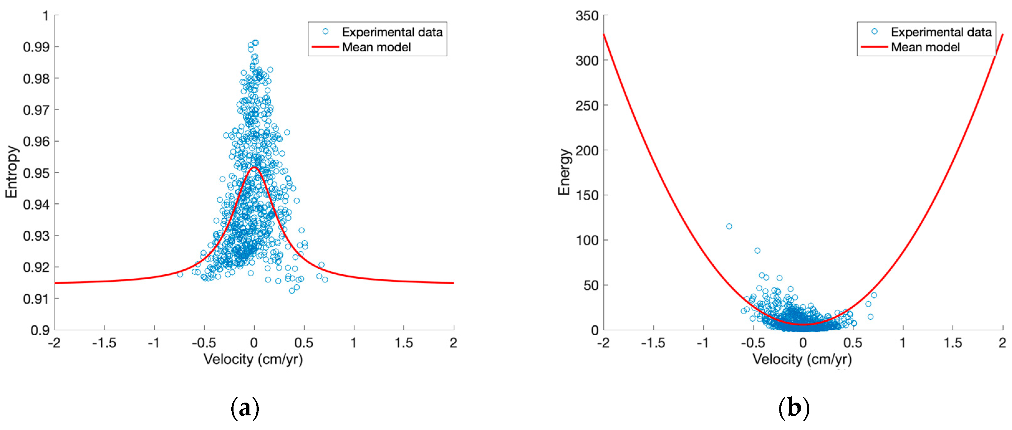
The entropy-energy dispersion can be further discussed by comparing two different periods to study the results before and after tunnel excavation. Given the complete dataset from 2011 to 2019, the following section distinguishes two periods of the same duration: 2011–2015 and 2015–2019. Figure 11 shows the correlation between the entropy-energy dispersion and the LOS velocity in the period from 2011 to 2015. Meanwhile, 
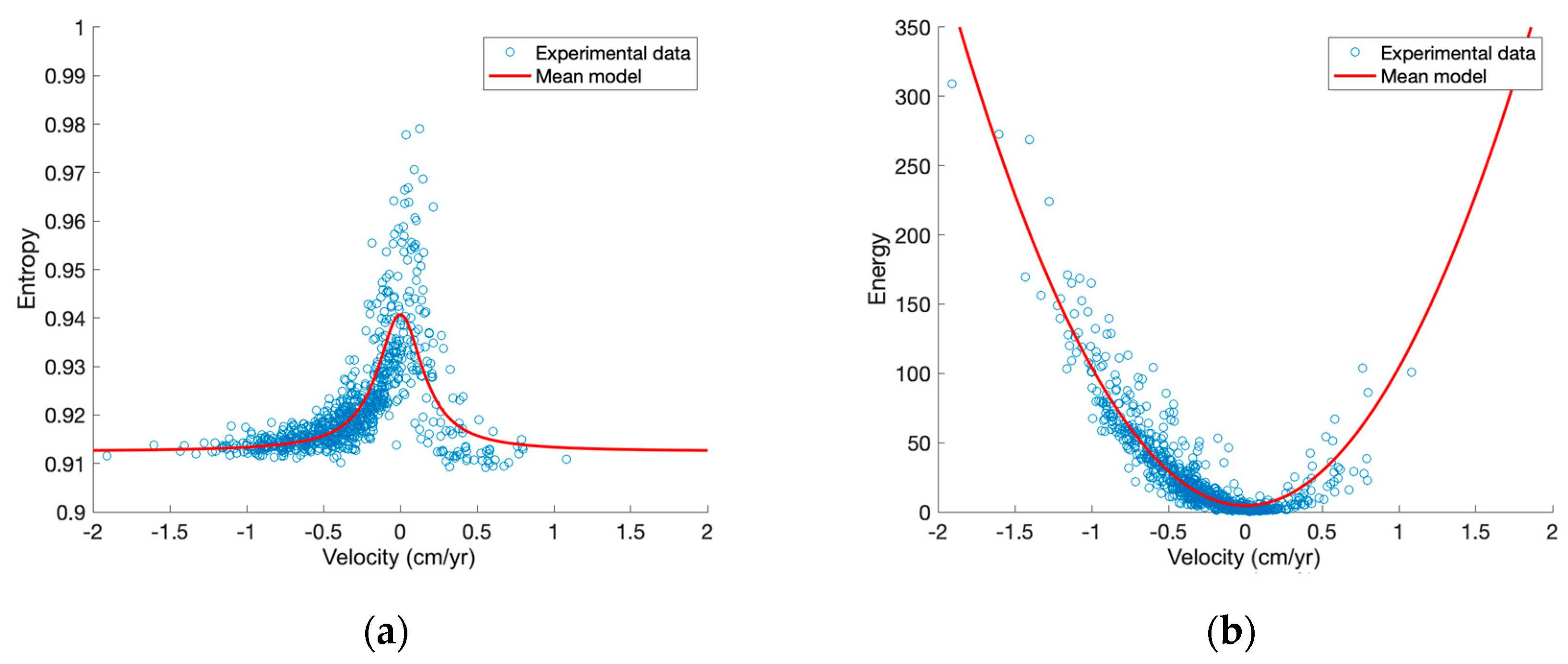
Figure 12 refers to the period from 2015 to 2019.
Figure 11a displays a higher level of scattering than Figure 12a. In addition, velocity values in the period 2011–2015 are more evenly dispersed when compared to the following period, and their intensity in the negative portion is lower, therefore significant subsidence is not observed. Consequently, the entropy-energy dispersion in the first period (Figure 13a) has fewer points on the low entropy–high energy branch with respect to Figure 13b, none of which reaches the limit of subsidence previously evaluated.
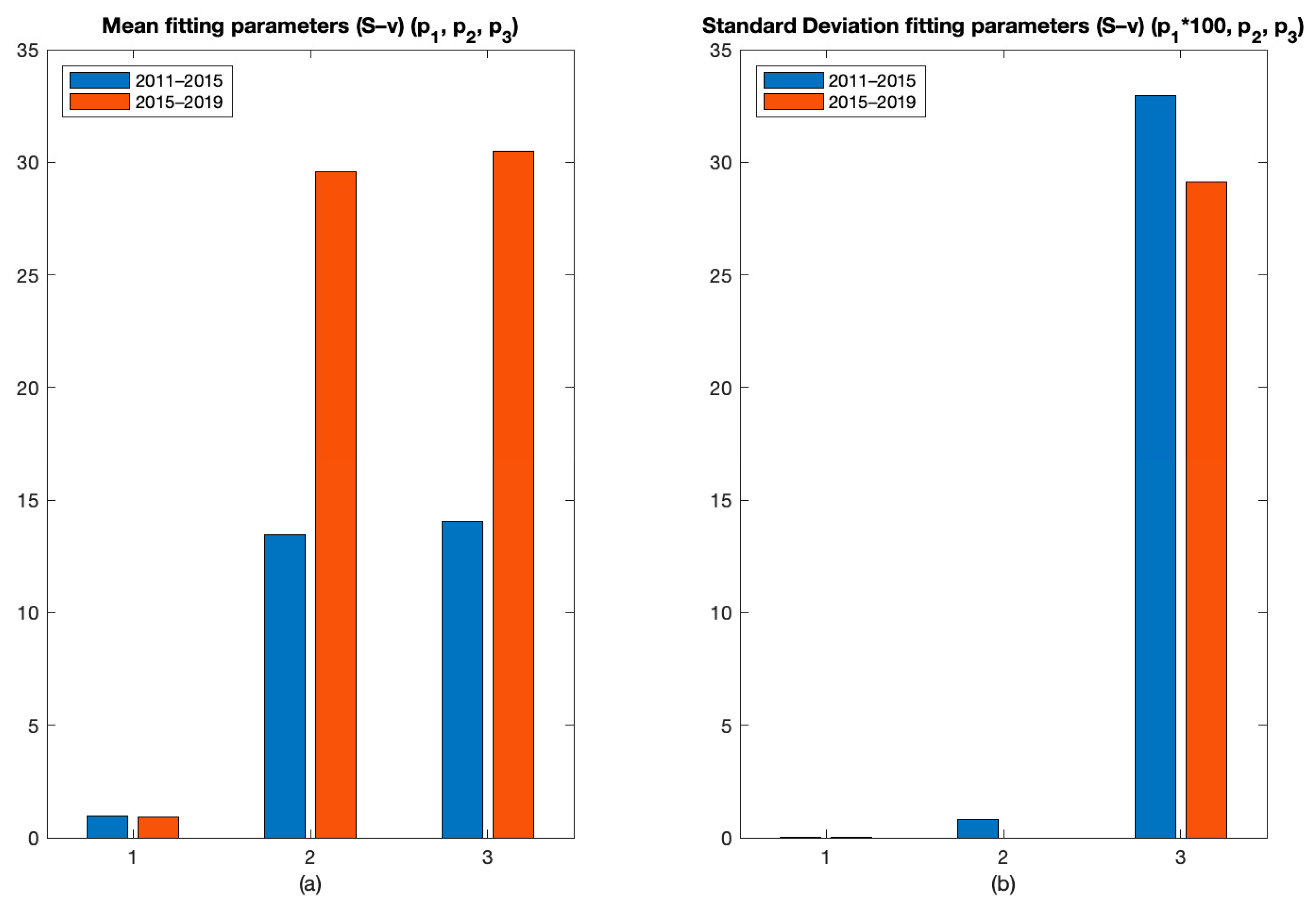
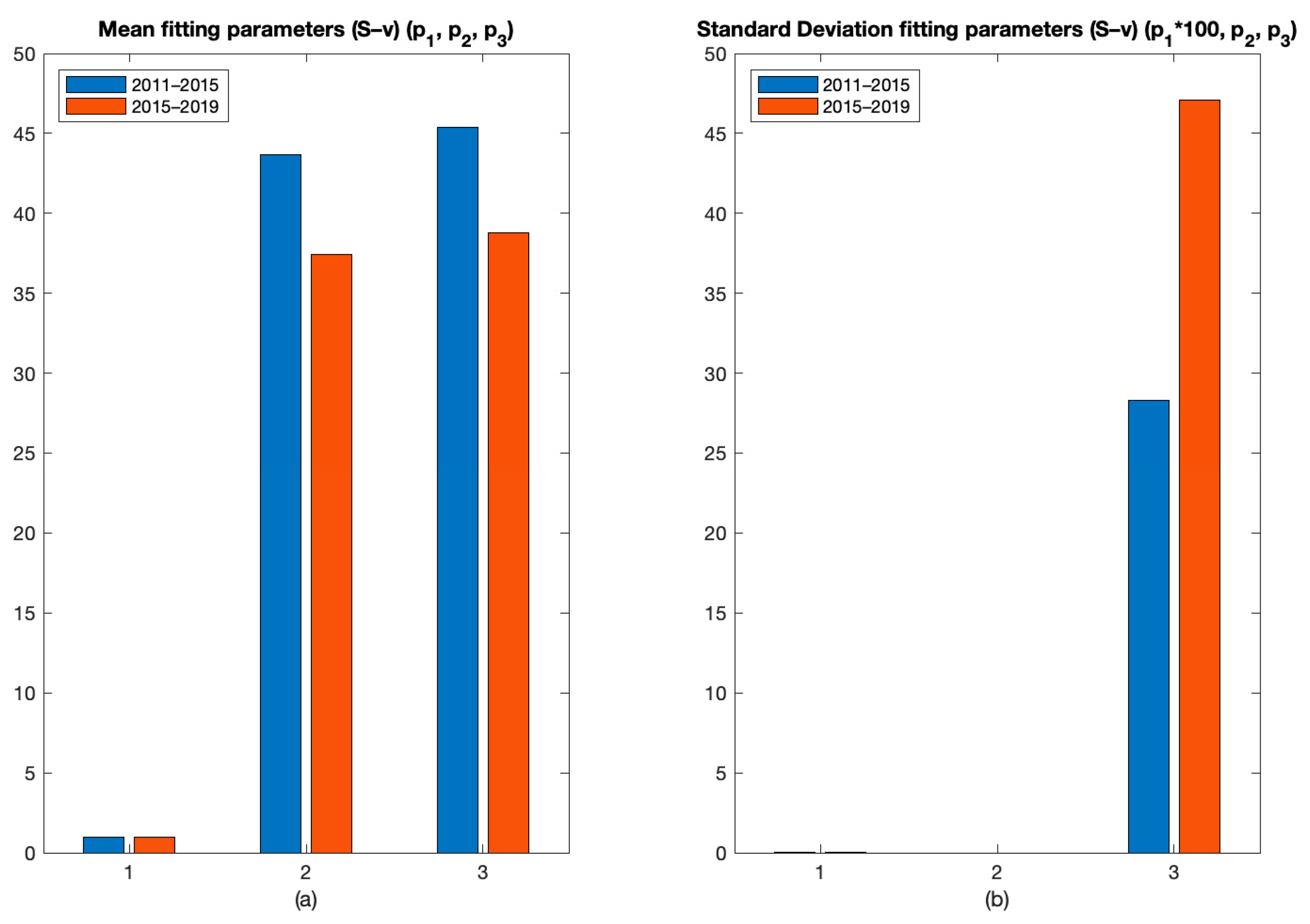
The comparison between the two periods is subsequently carried out by observing the variation in the parameters governing the fitting curves. A rational function of the second degree (Equation (2)) is used to fit the entropy-velocity dispersion ( S - v ) shown in Figure 11a and Figure 12a, and a nonlinear regression model is used, starting from null initial parameters. Thus, the mean model of the dispersion of the points is obtained. Subsequently, the regression model of the deviations from the mean model is studied, using the same type of equation:
S = p 1 p 2 v 2 + 1 p 3 v 2 + 1
It can be observed that Equation (2) is symmetrical with respect to the axis ( v = 0 ) . This condition derives from the intention to study the structural response in the range of small displacements, for which the structure is deemed to exhibit linear elastic behavior. In addition, it is assumed that the effect of settlements is also linear.
The first parameter of the mean model, which represents the value of the curve for null velocity, is subjected to a slight reduction, which is related to a global decrease in the system entropy in the second period. Instead, the ratio between p2 and p3 represents the limit value assumed by the function for high speed (in absolute value), normalized with respect to the p1 value. In addition, an increase in the values of p2 and p3, while maintaining the same ratio, corresponds to a reduction in the amplitude of the curve with respect to the vertical axis, as the inflection points tend to be closer to the axis ( v = 0 ). It occurs for the entropy in the second period, as shown by Figure 14a, where the two parameters increase, making the curve narrower with respect to the origin, so it tends toward the horizontal asymptotes more rapidly.
For the system’s variance (Figure 14b), the three parameters decrease from the first period to the second, reducing variance, especially for high velocity modules. It is worth noting that the parameters fitting guarantees positive variance.
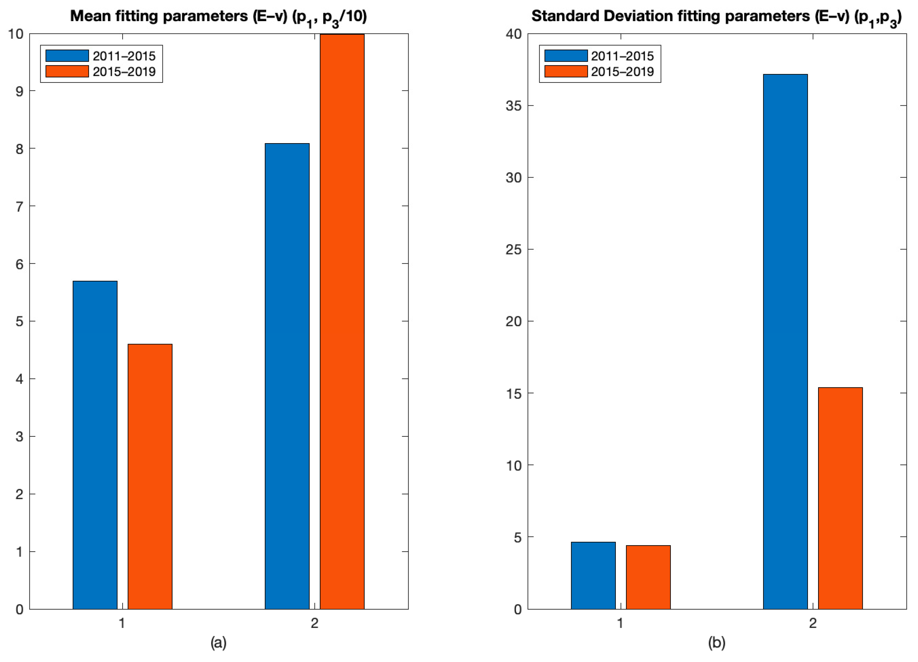
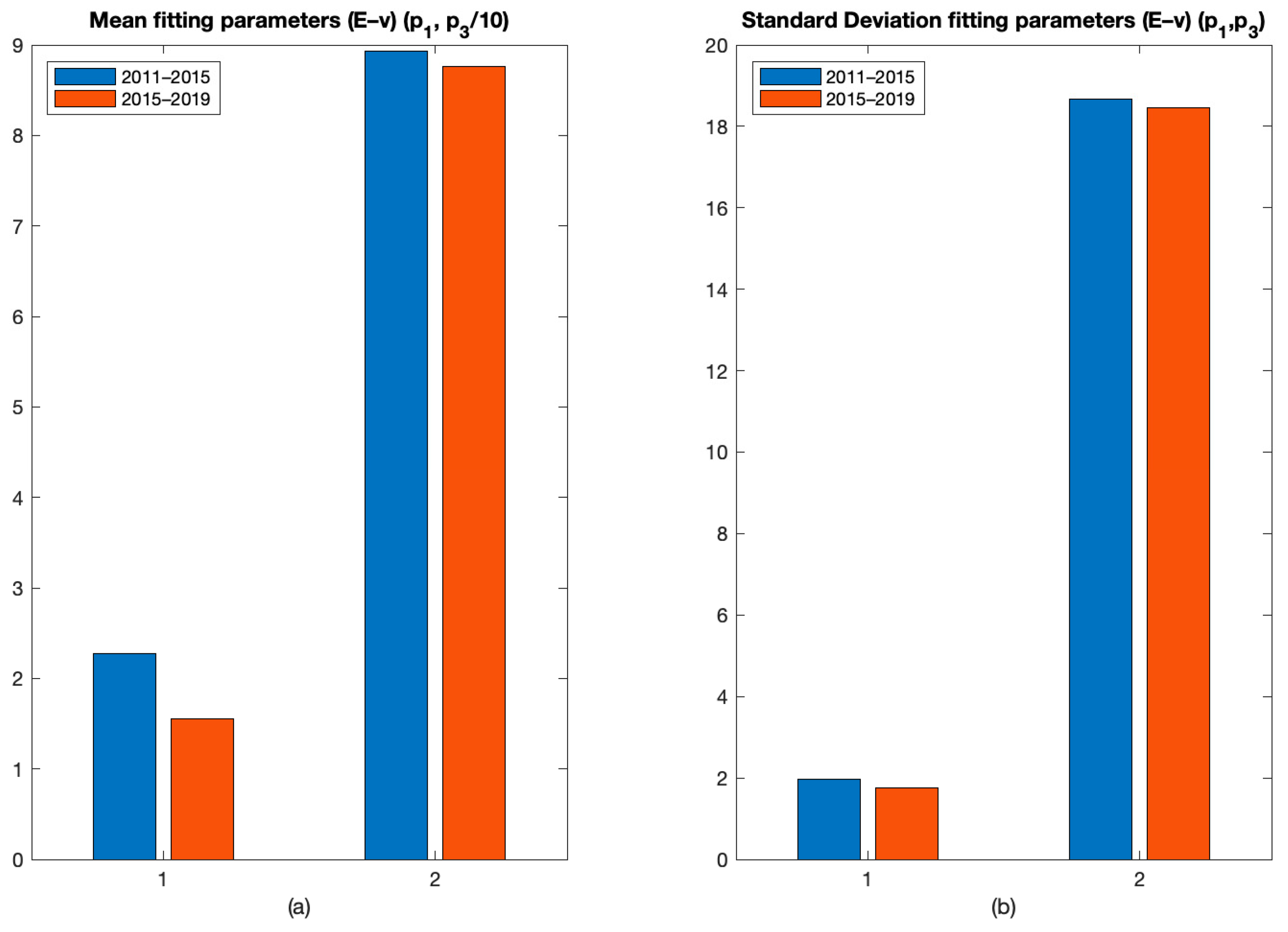
Figure 15 shows the parameters derived from a nonlinear regression model to construct the mean and standard deviation fittings of the energy-velocity ( E - v ) dispersion. A second-order polynomial model is used for the evaluation of the mean curve and the standard deviation, as a parabolic shape can easily be identified in the dispersion, especially in Figure 12b. As previously stated, the curves follow the hypothesis of linear elastic behavior; therefore, the vertices of the parabolic curves are fixed on the axis ( v = 0 ) .
The two average curves are similar, but higher energy values are reached in the second period at the same velocities. This effect is represented by the increase in the second parameter of the mean curve in Figure 15a.
As shown by the second parameter in Figure 15b, there is a significant reduction in the standard deviation between the first and second periods for higher velocity values in modulus.
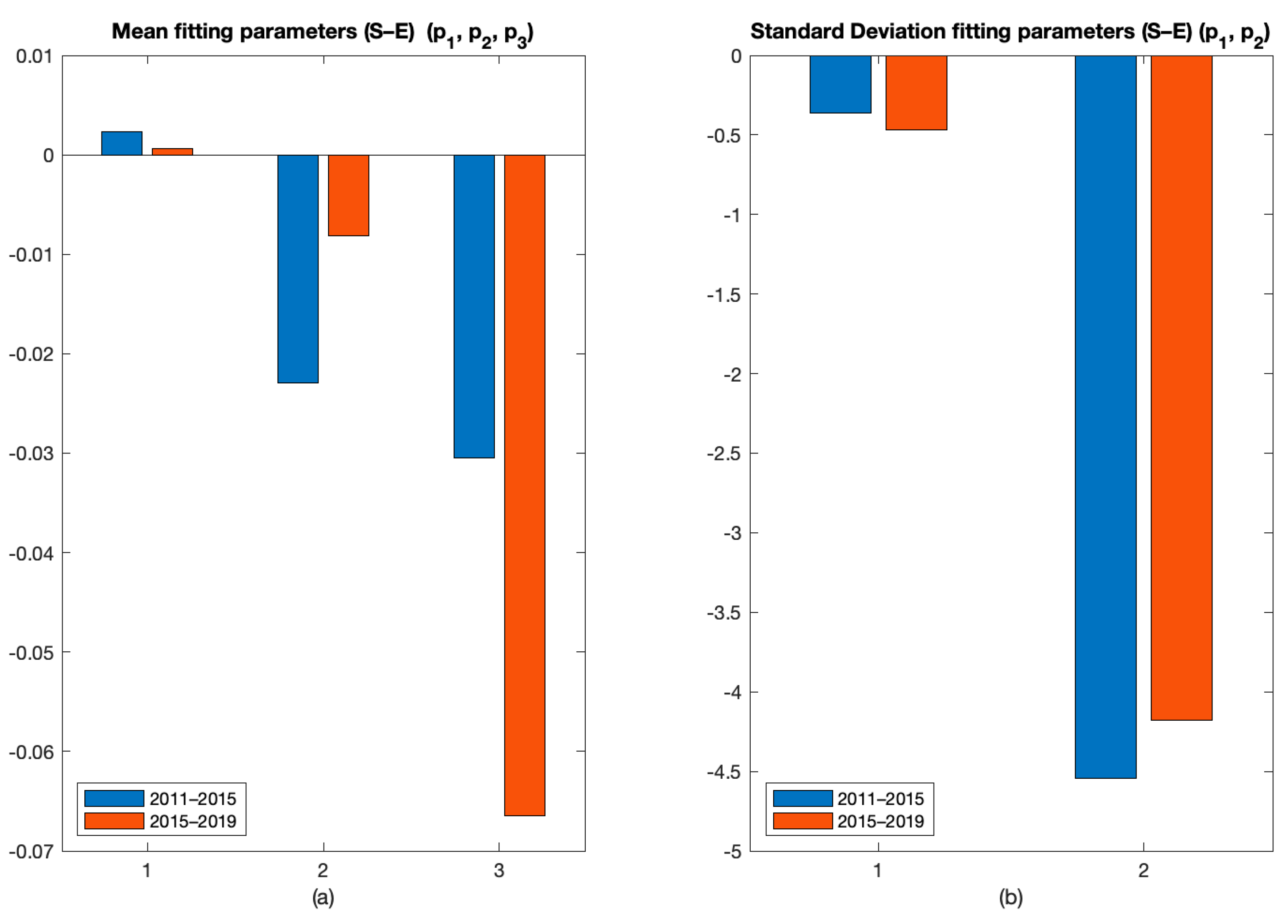
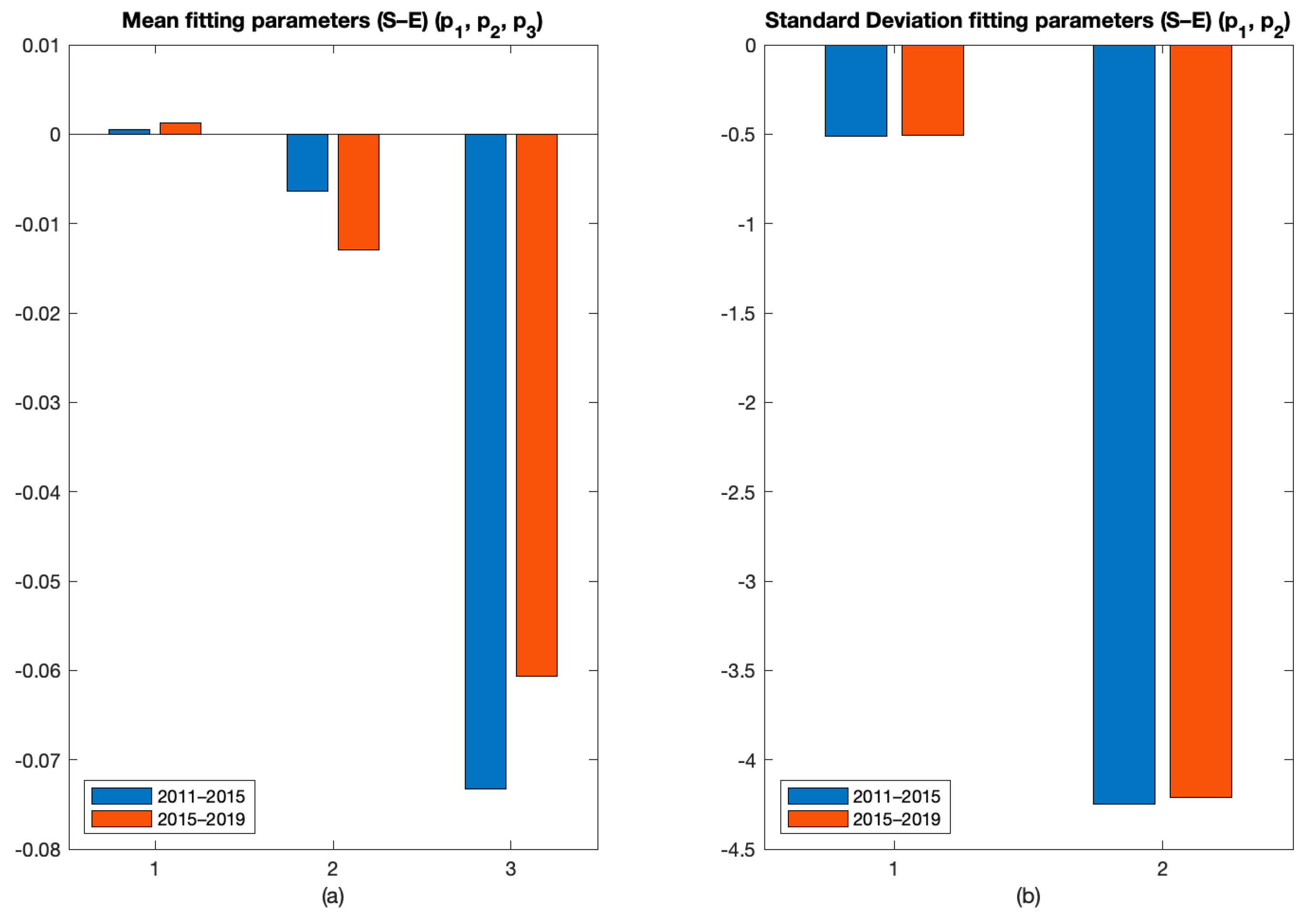
Figure 16 represents the parameters used to construct the mean and standard deviation model of the entropy-energy ( S - E ) dispersion. These parameters are evaluated using a nonlinear constrained minimization, where p 1 must be positive. A second-order polynomial model is used for the mean curve on a logarithmic scale, as given by
S = e x p ( p 1 ln E 2 + p 2 ln E + p 3 )
The value of p 3 represents the limit of the entropy, on the logarithmic scale, for an energy value that tends toward zero, so S tends toward e x p ( p 3 ) . The sign of p 1 expresses the concavity of the quadratic curve, while the ratio p 2 / 2 p 1 expresses its minimum. As mentioned above, a positive value of p 1 is enforced, in accordance with the physical meaning of the interpolated data. The decrease in the third parameter leads to a downward curve shift toward lower entropy values from the first period to the second. The module of the second parameter also decreases, leading to an increase in the curve slope on the logarithmic scale. Instead, the increase in the first parameter reduces the model’s curvature; therefore, the entropy decreases faster with the energy increase.
The curve tends to lower and shift toward higher energy values. The effect given by the first and third parameters is to obtain an approximately constant stretch at low entropy. A first-order polynomial curve models the standard deviation adopting the least-squares method. The parameters are shown in Figure 16b. The first parameter increases in modulus, representing a more rapid reduction in variance with increasing energy. In addition, the effect of the second parameter is added, causing an upward shift. Thus, for low energy values, a similar standard deviation is obtained in the two periods, whereas for lower entropy values, a lower deviation is obtained. The points result closer to the mean model.
Hence, in the second period (the one affected by excavations) there is an evident variation of the dispersions, underlined through the analysis of the fitting parameters. Moreover, the three dispersions analyzed display a reduction of the signal deviation from the mean model, which can be interpreted as lower uncertainty in the measures.

3.4. The Colosseum Case Study

The velocity-entropy-energy approach is also adopted to analyze another case study, i.e., the Colosseum, chosen for its importance in the area, considering its artistic, historical and cultural significance.
The period for which the data are available (2011–2019) does not include the excavation operations on the tunnel in the proximity of this structure, which are more recent. Nevertheless, it is possible to evaluate the application of the entropy-energy approach to a monumental structure with distinctive features to identify the outliers. In addition, since the area has not yet been subjected to excavation, it is possible to compare the dispersions in the two periods identified above to verify that no significant variations have occurred. It allows validating the correlation between the parameters’ variation and the effects of excavation on the building studied in previous sections.
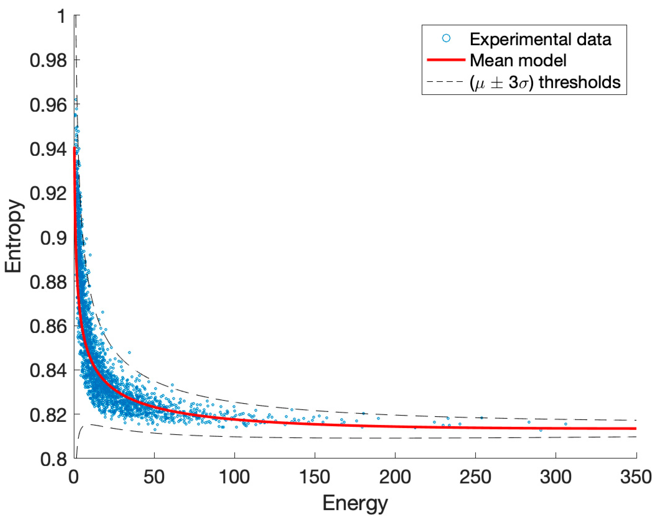
The first analysis concerns the entropy-energy distribution for the available period, shown in 
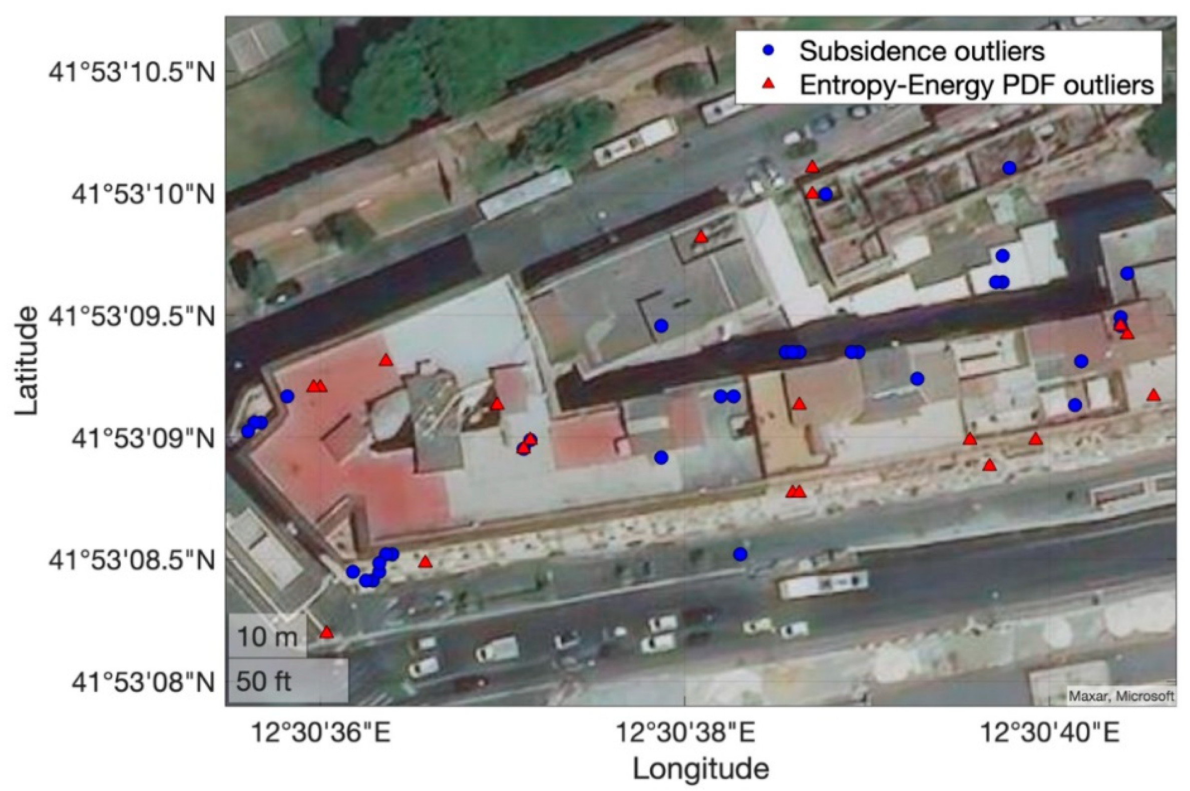
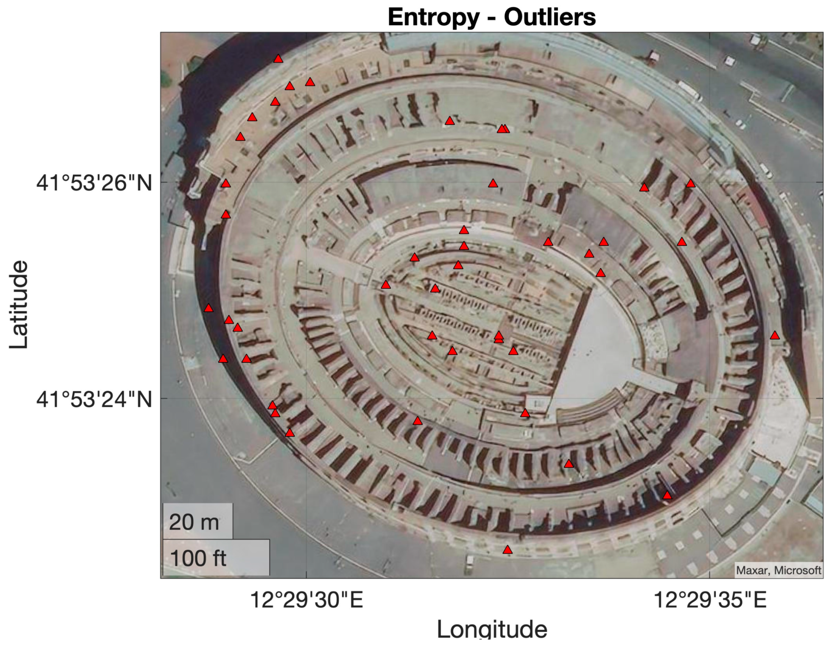
Figure 17. Defining the average model and the thresholds related to the standard deviation makes it possible to identify the outliers. It is observed that these points fall mainly on the high values of entropy and low energy. The localization of these points on the Colosseum, reported in Figure 18, highlights that they are distributed mainly on the base and in a cluster on the west end of the structure. Therefore, although further investigation is required, the presence of these outliers could be due to a differential behavior of the west end with respect to the whole system.
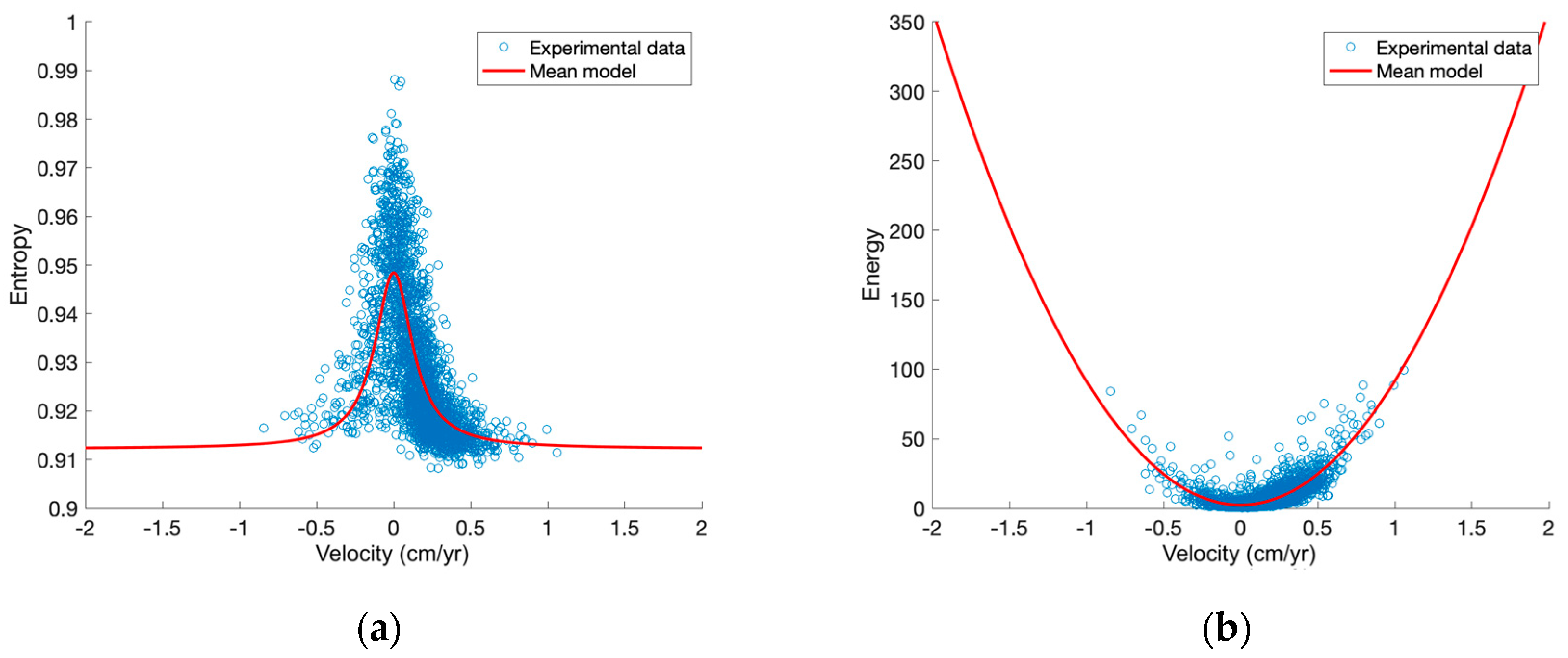
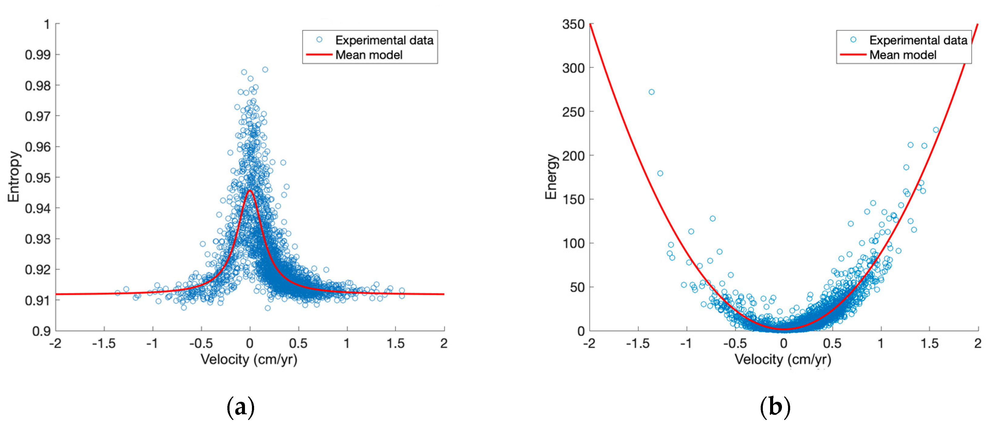
Analogously to the previous case study, the velocity, entropy and energy dispersions in the first and second half of the reference period are studied to highlight possible changes (Figure 19, Figure 20 and Figure 21). In addition, the parameters for the mean trends and standard deviation curves, respectively, are reported (Figure 22, Figure 23 and Figure 24).
The entropy-velocity ( S - v ) scatter in Figure 19a and Figure 20a shows a slight decrease in entropy for velocities with high modulus, represented by the change in the first parameter of the mean curve (Figure 22a). The energy-velocity ( E - v ) dispersion in Figure 19b and Figure 20b shows minimal changes in the average behavior, as shown by the parameters in Figure 23, though, in the second period, there are points showing higher velocity modules in the negative, as well as the positive section.
Finally, the entropy-energy ( S - E ) dispersions in Figure 21 exhibit similar characteristics, highlighted by the parameters in Figure 24. It can be observed that there is no significant change in the standard deviation of the points from the mean models. Moreover, as expected, the overall variation in the mean models is lower than in the previous case study. It should be noted that the Colosseum is only analyzed on an anthropogenic basis. Therefore, it would be appropriate to extend the analysis to also consider other aspects because of its complex hydrogeological configuration, which could lead to further data perturbations.

4. Conclusions

Recent developments in the acquisition of satellite interferometric data allow their integration to more traditional methods for Structural Health Monitoring purposes, providing additional insights that are often not available from in situ sensors and ensuring high spatial and temporal coverage. However, there are still some challenges related to their application because of the differences in the data gathered compared to the traditional on-site data.
The new kind of data requires the development of optimal representation techniques that may be used to identify anomalous behavior necessary to provide an interpretation and carry out damage identification. Therefore, this paper explores different approaches; the first one is the representation of direct quantities, such as the velocity along the LOS of the satellite, which allows the identification of slow territorial-scale phenomena, such as subsidence. A second representation concerns the indirect quantities of entropy and energy, which allows modeling the behavior of a system (e.g., single building, building complex, monumental structure).
These approaches are used to identify the effects of subsidence induced by the excavation of a new subway line in the urban area of Rome. In detail, the first representation highlights the presence of subsidence in the track’s proximity. The second one studies the effects on a smaller observation scale and identifies the outliers. The entropy-energy representation is compared to the LOS velocity to validate the results. It is observed that the points subjected to subsidence are distributed on a low-entropy and high-energy branch and are mainly characterized by low uncertainty, which can be interpreted as the signal of an actual movement.
In addition, the paper compares results obtained from two periods, before and after the start of excavation, studying parameter changes in the curve-fitting process. It highlights an evident variation in the signal response, especially in the variance parameters, indicating the presence of effects induced by tunnel construction.
The same procedure, applied to the Colosseum case study, does not show significant changes in the behavior of this monument, which was an expected result, given that its area had not been subjected to tunnel excavation during the analysis period. Furthermore, the ability of the entropy-energy representation to be applied to monumental structures is demonstrated, identifying the presence of outliers, i.e., points that should be further investigated, as they could also be related to anomalous structural and non-structural processes. Further studies are required to provide an objective interpretation of the outliers from the structural point of view. Nevertheless, future developments and the continuous increase in the quality of satellite data may allow the practical application of such information for SHM, leading to a low-cost, automated process for the study of large urban areas.

Author Contributions

Conceptualization, G.D., M.C., E.L., G.M., C.S. and R.C.; methodology, G.D., M.C., E.L., G.M., C.S. and R.C.; software, G.D., M.C., E.L., G.M., C.S. and R.C.; validation, G.D., M.C., E.L., G.M., C.S. and R.C.; formal analysis, G.D., M.C., E.L., G.M., C.S. and R.C.; investigation, G.D., M.C., E.L., G.M., C.S. and R.C.; resources, G.D., M.C., E.L., G.M., C.S. and R.C.; data curation, G.D., M.C., E.L., G.M., C.S. and R.C.; writing—original draft preparation, G.D.; writing—review and editing, G.D., M.C., E.L., G.M., C.S. and R.C.; visualization, G.D., M.C., E.L., G.M., C.S. and R.C.; supervision, M.C., E.L., G.M., C.S. and R.C.; project administration, M.C., E.L., G.M., C.S. and R.C.; funding acquisition, R.C. All authors have read and agreed to the published version of the manuscript.

Funding

This research was funded by “Progetto DPC-ReLUIS 2019–2021—WP 6 Monitoraggio e dati satellitari” (https://www.reluis.it/it/progetti-dpc-reluis/dpc-reluis-2019-2021.html, accessed on 25 January 2022).

Institutional Review Board Statement

Not applicable.

Informed Consent Statement

Not applicable.

Data Availability Statement

Data available from the authors upon reasonable request.

Acknowledgments

The authors want to acknowledge the “Progetto DPC-ReLUIS 2019–2021—WP 6 Monitoraggio e dati satellitari” for the provided experimental data.

Conflicts of Interest

The authors declare no conflict of interest.

References

  1. Farrar, C.R.; Worden, K. Structural Health Monitoring: A Machine Learning Perspective; John Wiley & Sons: Chichester, UK, 2012; ISBN 1-118-44321-7. [Google Scholar]
  2. Gili, P.; Civera, M.; Roy, R.; Surace, C. An unmanned lighter-than-air platform for large scale land monitoring. Remote Sens. 2021, 13, 2523. [Google Scholar] [CrossRef]
  3. Campbell, J.B.; Wynne, R.H. Introduction to Remote Sensing; Guilford Press: New York, NY, USA, 2011; ISBN 1-60918-177-8. [Google Scholar]
  4. Forster, B. An examination of some problems and solutions in monitoring urban areas from satellite platforms. Int. J. Remote Sens. 1985, 6, 139–151. [Google Scholar] [CrossRef]
  5. Curlander, J.C.; McDonough, R.N. Synthetic Aperture Radar; Wiley: New York, NY, USA, 1991; Volume 11. [Google Scholar]
  6. Rodriguez, E.; Martin, J. Theory and design of interferometric synthetic aperture radars. IEE Proc. F Radar Signal Process. 1992, 139, 147–159. [Google Scholar] [CrossRef]
  7. Bonano, M.; Manunta, M.; Pepe, A.; Paglia, L.; Lanari, R. From previous C-band to new X-band SAR systems: Assessment of the DInSAR mapping improvement for deformation time-series retrieval in urban areas. IEEE Trans. Geosci. Remote Sens. 2013, 51, 1973–1984. [Google Scholar] [CrossRef]
  8. Cigna, F.; Lasaponara, R.; Masini, N.; Milillo, P.; Tapete, D. Persistent scatterer interferometry processing of COSMO-SkyMed StripMap HIMAGE Time series to depict deformation of the historic centre of Rome, Italy. Remote Sens. 2014, 6, 12593–12618. [Google Scholar] [CrossRef] [Green Version]
  9. Zhu, M.; Wan, X.; Fei, B.; Qiao, Z.; Ge, C.; Minati, F.; Vecchioli, F.; Li, J.; Costantini, M. Detection of building and infrastructure instabilities by automatic spatiotemporal analysis of satellite SAR interferometry measurements. Remote Sens. 2018, 10, 1816. [Google Scholar] [CrossRef] [Green Version]
  10. Arangio, S.; Calò, F.; Di Mauro, M.; Bonano, M.; Marsella, M.; Manunta, M. An application of the SBAS-DInSAR technique for the assessment of structural damage in the city of Rome. Struct. Infrastruct. Eng. 2014, 10, 1469–1483. [Google Scholar] [CrossRef]
  11. Bozzano, F.; Esposito, C.; Mazzanti, P.; Patti, M.; Scancella, S. Imaging multi-age construction settlement behaviour by advanced SAR interferometry. Remote Sens. 2018, 10, 1137. [Google Scholar] [CrossRef] [Green Version]
  12. Macchiarulo, V.; Milillo, P.; Blenkinsopp, C.; Reale, C.; Giardina, G. InSAR monitoring of regional infrastructure networks. In Proceedings of the 2021 IEEE International Geoscience and Remote Sensing Symposium IGARSS, Brussels, Belgium, 11–16 July 2021; pp. 6233–6236. [Google Scholar]
  13. Di Carlo, F.; Miano, A.; Giannetti, I.; Mele, A.; Bonano, M.; Lanari, R.; Meda, A.; Prota, A. On the integration of multi-temporal synthetic aperture radar interferometry products and historical surveys data for buildings structural monitoring. J. Civ. Struct. Health Monit. 2021, 11, 1429–1447. [Google Scholar] [CrossRef]
  14. Tang, P.; Chen, F.; Zhu, X.; Zhou, W. Monitoring cultural heritage sites with advanced multi-temporal InSAR technique: The case study of the summer palace. Remote Sens. 2016, 8, 432. [Google Scholar] [CrossRef] [Green Version]
  15. Milillo, P.; Giardina, G.; DeJong, M.J.; Perissin, D.; Milillo, G. Multi-temporal InSAR structural damage assessment: The London crossrail case study. Remote Sens. 2018, 10, 287. [Google Scholar] [CrossRef] [Green Version]
  16. Lenticchia, E.; Miraglia, G.; Ceravolo, R. Exploring problems and prospective of satellite interferometric data for the seismic structural health monitoring of existing buildings and architectural heritage. In Proceedings of the 10th International Conference on Structural Health Monitoring of Intelligent Infrastructure, SHMII 10, Porto, Portugal, 30 June–2 July 2021. [Google Scholar]
  17. Talledo, D.A.; Miano, A.; Bonano, M.; Di Carlo, F.; Lanari, R.; Manunta, M.; Meda, A.; Mele, A.; Prota, A.; Saetta, A. Satellite radar interferometry: Potential and limitations for structural assessment and monitoring. J. Build. Eng. 2021, 46, 103756. [Google Scholar] [CrossRef]
  18. ReLUIS. Pubblicata la Prima Versione delle Linee Guida per l’Utilizzo dei Dati Interferometrici Satellitari Ai Fini dell’interpretazione del Comportamento Strutturale delle Costruzioni. Available online: https://www.reluis.it (accessed on 15 November 2021).
  19. Agenzia Spaziale Italiana (ASI). Home Page. Available online: https://www.asi.it (accessed on 15 November 2021).
  20. Lanari, R.; Mora, O.; Manunta, M.; Mallorquí, J.J.; Berardino, P.; Sansosti, E. A small-baseline approach for investigating deformations on full-resolution differential SAR interferograms. IEEE Trans. Geosci. Remote Sens. 2004, 42, 1377–1386. [Google Scholar] [CrossRef]
  21. Ferretti, A.; Guarnieri, A.M.; Prati, C.; Rocca, F. InSAR Principles: Guidelines for SAR Interferometry Processing and Interpretation; ESA Pubblications ESTEC: Noordwijk, The Netherlands, 2007. [Google Scholar]
  22. Tapete, D.; Cigna, F. COSMO-SkyMed SAR for detection and monitoring of archaeological and cultural heritage sites. Remote Sens. 2019, 11, 1326. [Google Scholar] [CrossRef] [Green Version]
  23. Italian Space Agency. ASI COSMO-SkyMed Mission and Products Description. In Doc. N°ASI-CSM-PMG-NT-001, 8 July 2019, Issue 3; Italian Space Agency: Rome, Italy, 2019. [Google Scholar]
  24. Metro C, S.P.A. Metro C—Il GC Che Sta Realizzando la Linea C. Available online: https://metrocspa.it (accessed on 15 November 2021).
  25. Shannon, C.E. A mathematical theory of communication. Bell Syst. Tech. J. 1948, 27, 379–423. [Google Scholar] [CrossRef] [Green Version]
  26. Farrar, C.; Park, G.; Worden, K. Complexity: A New Axiom for Structural Health Monitoring? Los Alamos National Laboratory: Los Alamos, NM, USA, 2010. [Google Scholar]
  27. Metro C, S.P.A. Metro C: Un VIaggio Nella Storia. La Stazione Amba Aradam/Ipponio. Available online: https://metrocspa.it/blog/metro-c-un-viaggio-nella-storia-la-stazione-amba-aradam-ipponio/ (accessed on 29 December 2021).
  28. Miliziano, S.; de Lillis, A. Predicted and Observed settlements induced by the mechanized tunnel excavation of metro line c near S. Giovanni station in Rome. Tunn. Undergr. Space Technol. 2019, 86, 236–246. [Google Scholar] [CrossRef]
  29. D’Aranno, P.J.; Gizzi, F.; Marsella, M.; Scifoni, S.; Scutti, M.; Sonnessa, A.; Bonano, M.; Manunta, M. Understanding the effects of tunneling on buildings by analyzing dinsar data: The case of the new subway in Rome, Italy. In Proceedings of the 1st IMEKO TC4 International Workshop on Metrology for Geotechnics, MetroGeotechnics, Benevento, Italy, 17–18 March 2016. [Google Scholar]
Figure 1. Map showing the T3 section of the Line C subway and the numerosity of points obtained by satellite interferometry over the analyzed urban area of Rome (Italy).
Applsci 12 01658 g001
Figure 2. Map showing the T3 section of the Line C subway, the stations, the inter-tract shafts and the interaction with the other subway lines, Rome (Italy), edited from (https://goo.gl/maps/zPUUjveLSWBzj7nC9, accessed on 28 January 2022), [27].
Applsci 12 01658 g002
Figure 3. Map showing the dispersion of the average annual velocity along the LOS in the period from 2017 to 2019. The route in black refers to the part already under construction; the route in grey refers to parts not yet built.
Applsci 12 01658 g003
Figure 4. Map showing the dispersion of the average annual velocity along the LOS in the period from 2014 to 2016.
Applsci 12 01658 g004
Figure 5. Map showing the points with velocity outside the imposed lower threshold, with respect to the subway route and the proximity boundaries.
Applsci 12 01658 g005
Figure 6. View of the analyzed building on the map, at the intersection of Via Emanuele Filiberto and Via Castrense (https://www.google.it/maps/place/41%C2%B053’09.2%22N+12%C2%B030’36.6%22E/@41.8835837,12.5093078,320a,35y,39.39t/data=!3m1!1e3!4m5!3m4!1s0x0:0xfe6a6f12a7bebc20!8m2!3d41.885885!4d12.510169, accessed on 25 January 2022).
Applsci 12 01658 g006
Figure 7. Entropy-energy dispersion and probability distribution function of the analytical model for a building complex near San Giovanni station.
Applsci 12 01658 g007
Figure 8. Correlation between LOS velocity and entropy-energy dispersion in the period from 2017 to 2019 for a building complex near San Giovanni station: (a) Entropy-velocity dispersion; (b) Energy-velocity dispersion.
Applsci 12 01658 g008
Figure 9. Entropy-energy dispersion for a building complex near San Giovanni station in the period from 2017 to 2019.
Applsci 12 01658 g009
Figure 10. Map showing the experimental data for a building complex near San Giovanni station. The locations where subsidence is most emphasized and the entropy-energy outliers are highlighted.
Applsci 12 01658 g010
Figure 11. Correlation between LOS velocity and entropy-energy dispersion in the period from 2011 to 2015 for a building complex near San Giovanni station: (a) Entropy-velocity dispersion; (b) Energy-velocity dispersion.
Applsci 12 01658 g011
Figure 12. Correlation between LOS velocity and entropy-energy dispersion in the period from 2015 to 2019 for a building complex near San Giovanni station: (a) Entropy-velocity dispersion; (b) Energy-velocity dispersion.
Applsci 12 01658 g012
Figure 13. Entropy-energy dispersion, mean model and thresholds for a building complex near San Giovanni station: (a) period from 2011 to 2015; (b) period from 2015 to 2019.
Applsci 12 01658 g013
Figure 14. Fitting parameters of the entropy-velocity dispersions in the two periods for a building complex near San Giovanni station: (a) parameters of the mean model; (b) parameters of the standard deviation model.
Applsci 12 01658 g014
Figure 15. Fitting parameters of the energy-velocity dispersions in the two periods for a building complex near San Giovanni station: (a) parameters of the mean model; (b) parameters of the standard deviation model.
Applsci 12 01658 g015
Figure 16. Fitting parameters of the entropy-energy dispersions in the two periods for a building complex near San Giovanni station: (a) parameters of the mean model; (b) parameters of the standard deviation model.
Applsci 12 01658 g016
Figure 17. Entropy-energy dispersion and mean model for the Colosseum, from 2011 to 2019.
Applsci 12 01658 g017
Figure 18. Map showing the outliers evaluated from the entropy-energy PDF for the Colosseum.
Applsci 12 01658 g018
Figure 19. Correlation between LOS velocity and entropy-energy dispersion for the Colosseum in the period from 2011 to 2015: (a) Entropy-velocity dispersion; (b) Energy-velocity dispersion.
Applsci 12 01658 g019
Figure 20. Correlation between LOS velocity and entropy-energy dispersion for the Colosseum in the period from 2015 to 2019: (a) Entropy-velocity dispersion; (b) Energy-velocity dispersion.
Applsci 12 01658 g020
Figure 21. Entropy-energy dispersion, mean model and thresholds for the Colosseum: (a) period from 2011 to 2015; (b) period from 2015 to 2019.
Applsci 12 01658 g021
Figure 22. Fitting parameters of the entropy-velocity dispersions in the two periods for the Colosseum: (a) parameters of the mean model; (b) parameters of the standard deviation model.
Applsci 12 01658 g022
Figure 23. Fitting parameters of the energy-velocity dispersions in the two periods for the Colosseum: (a) parameters of the mean model; (b) parameters of the standard deviation model.
Applsci 12 01658 g023
Figure 24. Fitting parameters of the entropy-energy dispersions in the two periods for the Colosseum: (a) parameters of the mean model; (b) parameters of the standard deviation model.
Applsci 12 01658 g024
Publisher’s Note: MDPI stays neutral with regard to jurisdictional claims in published maps and institutional affiliations.

