Article

A Comparative Study of a Fully-Connected Artificial Neural Network and a Convolutional Neural Network in Predicting Bridge Maintenance Costs

Department of Bridge and Tunnel Engineering, School of Civil Engineering, Southwest Jiaotong University, No. 111, North 1st Section of Second Ring Road, Jinniu District, Chengdu 610031, China
*
Author to whom correspondence should be addressed.
Submission received: 27 February 2022 / Revised: 23 March 2022 / Accepted: 29 March 2022 / Published: 1 April 2022

Abstract

:
The cost assessment of bridge maintenance is a difficult topic to study, but it is critical for a bridge life cycle cost analysis. The maintenance costs sample database was established in this study according to actual engineering data, and a bridge maintenance cost prediction model was developed using a fully-connected artificial neural network (ANN) and convolutional neural network (CNN), respectively. First, eight main factors affecting maintenance costs were evaluated based on the random forest method, and the evaluation results were verified by an exploratory data analysis. The original data were then screened based on the isolation forest principle, and the recent gross domestic product (GDP) growth rate was used to illustrate the relationship between economic development and bridge maintenance costs. Finally, these two neural networks were used to establish maintenance cost prediction models, respectively. The results from the two models were compared and their prediction accuracies were analyzed. The prediction performance of the CNN model for bridge maintenance costs was found to be better than that of the traditional fully-connected ANN model. The results of this study will enhance the opportunity for bridge managers to balance lifecycle maintenance costs.

1. Introduction

Bridges are important parts of transportation infrastructure; the expected service life of a bride is (at least) several decades and possibly more than 100 years. Bridges need to be maintained continuously to ensure their safety and applicability during the service period. The 2021 Infrastructure Report Card by the American Society of Civil Engineers (ASCE) states that about 7.5% of bridges in the USA were structurally deficient in 2020 [1]. An estimated USD 123 billion was invested into bridge maintenance in the USA, at all levels of government, in 2019 [2]. In 2016, there were 86,000 bridges in need of maintenance in China, which is approximately 10% of the total number of bridges [3], roughly equivalent to the proportion of structurally deficient bridges in the USA. The total number of highway bridges in China reached 912,800 at the end of 2020, which brought tremendous pressure on bridge maintenance [4]. Both China and the USA are facing difficulties in having such a large number of aging bridges. Maintenance is arduous and requires huge capital investments. Correct maintenance cost estimations are important in the planning of bridge maintenance [5].
Current maintenance cost studies primarily focus on the optimization of cost-oriented maintenance scenarios. Barone and Frangopol considered the interactions among components in the system, and selected the most cost-effective maintenance measures according to detection results and preset damage threshold [6]. Sabatino et al. combined maintenance costs, failure losses, and choice preferences to optimize multiple objectives in the maintenance planning simultaneously, with the goal of finding a set of Pareto optimal solutions [7]. Condition states and reliability indicators were defined as performance indicators, and a multilinear model was used to describe the degradation process of performance indicators under different maintenance scenarios. Ghodoosi et al. selected the most cost-effective one by comparing different maintenance scenarios based on a genetic algorithm engine [8].
Many domestic and foreign researchers have carried out extensive research in the cost assessment of bridge maintenance theory, making significant progress. There are cost estimation methods based on numerical analyses, for example, maintenance cost estimations based on the bridge performance degradation model and binary programming algorithm [9], bridge maintenance cost allocation based on the priority index [10], prediction of daily maintenance costs of bridges based on linear regression and time series analyses [11], and the cost assessment of bridge maintenance based on system reliability analyses and multiple regression algorithms [12]. Such evaluation models are established based on the statistical analysis and parametric analysis results of maintenance costs. As for their advantages: they do not require large amounts of samples and the evaluation of maintenance costs could be achieved with fewer computational steps/computational effort. However, these models have some drawbacks. For example, the model prediction accuracy is not high because the parametric analysis does not fully learn the characteristics of the data.
At the same time, there are cost prediction studies based on data analyses and the intelligent algorithm. For example, Bayzid et al. established a cost prediction model through the particle swarm algorithm based on big data analysis. This method can predict the short-term maintenance costs of the structure under the current performance [13]. Echaveguren and Dechent allocated the costs of bridge maintenance based on prioritization indices, according to the condition, strategic importance, and vulnerability of the bridge. This method involves simple/a small amount of calculations, which is helpful in short-term maintenance decision-making [14]. Shi et al. established a database of the daily maintenance costs of bridges in the United States, with the logarithm of the maintenance cost as a dependent variable and the service life of the bridge as an independent variable, and they proposed a prediction model based on a backtracking search algorithm [15]. Zhu et al. proposed a decision-making method based on performance detection and maintenance cost records of Chinese bridges, and used an annealing algorithm to evaluate the future maintenance costs and expected losses of bridges [16]. Then, the genetic algorithm was used to find the decision-making scheme with the lowest maintenance costs in the whole life cycle of the bridge. This is a decision-making method combining bridge performance and costs but does not explain the quantitative relationship between bridge performance and maintenance costs. Most of the existing bridge maintenance cost prediction models are based on the maintenance cost prediction of a single type of input indicator with a small sample base. This affects the applicability and generalization ability of the model. Bridge maintenance cost prediction is a typical and complex nonlinear regression problem. The prediction models established based on traditional statistical analysis methods and simple data-driven intelligent algorithms have certain defects in prediction accuracy and generalization performance. It is necessary to analyze, in detail, the degree of influence of many factors that affect the costs of bridge maintenance and, on this basis, use intelligent algorithms to deeply learn and extract the characteristics of actual engineering data. Thus, a set of computing processes and methods that combine data preprocessing, influencing factor analyses, and intelligent predictions are established. An effective “reference” for bridge managers would involve quantitative prediction of bridge maintenance costs using conventional bridge maintenance data.
Based on the above, a database of the maintenance costs in bridges was constructed in this study, based on practical engineering data, containing the maintenance cost samples of 268 bridges in Chinese inland and coastal areas. The database includes many factors that affect maintenance costs, for example bridge location, bridge technical condition, bridge maintenance time. The fully-connected ANN and CNN were used to establish the intelligent prediction model of maintenance costs, respectively, and the prediction accuracies were compared. We also propose a new method to optimize bridge life cycle maintenance costs and predict the time-varying law of maintenance cost.

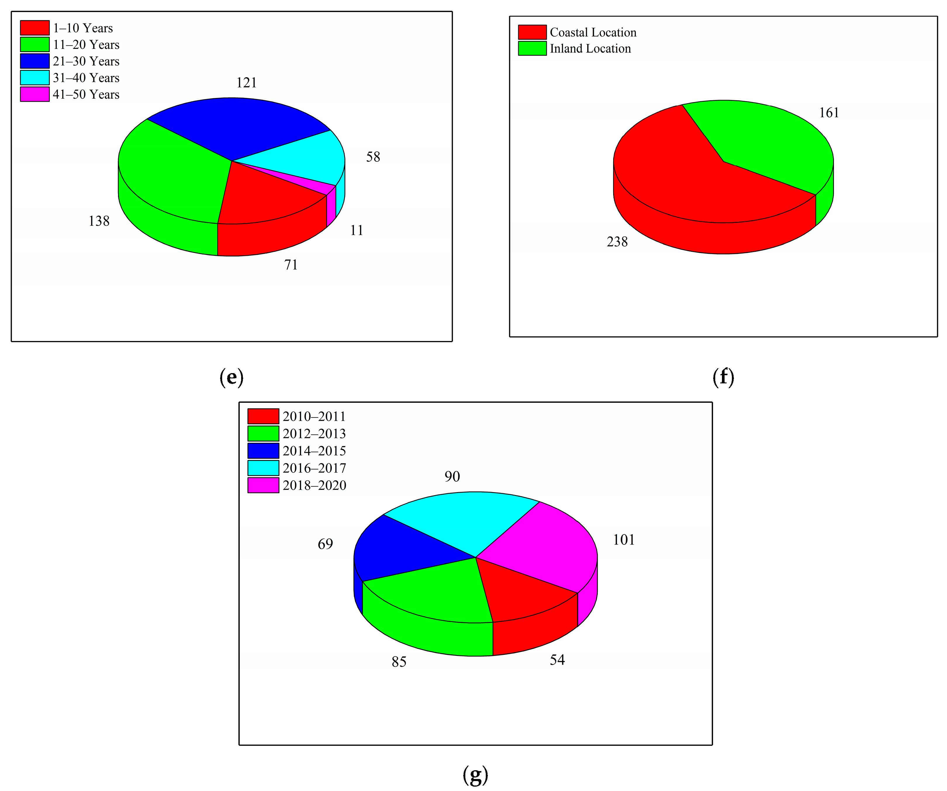
2. Bridge Maintenance Cost Database

A variety of external factors could affect the maintenance costs of bridges [17]. The bridge maintenance-related costs in China’s coastal and inland areas are highly discrete and influenced by multiple factors. The obtained data are classified according to the seven main factors that affect the maintenance costs (maintenance time, bridge technical condition, bridge location, bridge age, bridge grade, superstructure, highway grade). Classifications of all data in the database are shown in Figure 1. The database contains a total of 399 maintenance cost samples.
The classification standards of highway grades are based on the Chinese “Technical Standard of Highway Engineering (JTG B01-2019)” and are divided according to the design service life of the highway on which the bridge is located [18]. The details are presented in Table 1. The technical condition grades are classified according to the Chinese “Highway Performance Assessment Standards (JTG 5210-2018)” and are divided according to the weighted score of the overall technical conditions of the bridge [19]. The details are presented in Table 2; “Highway Bridge Design standard” is the reference standard for classification of bridge grades and the details are presented in Table 3 [20].
In China, bridge maintenance costs are considered public expenditures. All levels of government investments in bridge maintenance are affected by economic development. GDP growth rate was used as the eighth influencing factor in this study in order to assess the impact of economic effects on investments in bridge maintenance. GDP growth rates from previous years could be queried on government websites; its predicted values were calculated using the prediction models developed by economists [21]. The prediction model for Chinese GDP growth rate used in this study was established by Jiang [22]. The values of the Chinese GDP growth rate in past years are presented in Figure 2 [23].

3. Neural Network-Based Bridge Maintenance Cost Prediction Framework

In recent years, with the development of computer technology, neural networks have become more mature and diverse. For example, the fully-connected ANN is widely used to solve engineering problems. The deep learning proposed by Geoffrey Hinton in 2006 broke the limitations of traditional neural networks on the number of layers and further broadened the application scope of neural networks [24].
Therefore, this section introduces a comparative study of a fully-connected ANN and CNN for predicting bridge maintenance costs. The calculation framework of the two models is shown in Figure 3. It was necessary to preprocess the dataset of bridge maintenance costs prior to establishing the neural network model. This included an exploratory data analysis, selection of input indicators, and sample screening. The database was divided into a training set and a test set, which were used to train the neural network model and verify the prediction performance of the model, respectively.

3.1. Selecting Input Indicators Based on Random Forest

Random forest is a classification index test method based on decision trees. It is widely applied and achieves good results in the index selection of low feature dimensions and low sample size data [25,26]. The VIM is used to express the importance of indicators, and the Gini index [27], which represents the probability that a randomly selected sample in the sample set has been classified by mistake, is used to calculate the VIM value.
Suppose that there are n indicators X1, X2, X3Xn, the Gini variable importance measure of each indicator Xj is calculated and represented by V I M j ( G i n i ) , which represents the average change of node splitting impurity in the j-th variable in all decision trees in the random forest [28]. The detailed calculation process of V I M j ( G i n i ) is as follows:
(1)
Calculate the Gini index of the node m in a certain category K. The formula for calculating the Gini is:
G I m = k = 1 K P m k ^ ( 1 P m k ^ )
where K is the number of categories in the sample set and P m k ^ is the estimated probability that the sample of node m belongs to the k-th category; when the sample belongs to one of categories, K = 2.
(2)
The decision trees in the random forest used in this study only had two branches. Therefore, the Gini index of node m could be calculated as:
G I m = 2 P m ^ ( 1 P m ^ )
where P m ^ is the estimated probability that the sample belongs to any category at node m.
(3)
Calculate the VIM value of node m. The importance of indicator Xj at node m; that is, the variable quantity in the Gini index before and after the branch at node m is:
V I M j m ( G i n i ) = G I m G I l G I r
where G I l and G I r represent the Gini indexes of two new nodes split by node   m .
(4)
Calculate the VIM value of indicator X j in the random forest. If the indicator X j appears M times i-th in the tree, the importance of the indicator X j in the i-th tree is:
V I M i j ( G i n i ) = m = 1 M V I M j m ( G i n i )
The VIM of the indicator X j in the random forest is defined as:
V I M i j ( G i n i ) = 1 n i = 1 n V I M i j ( G i n i )
where n is the number of decision trees in the random forest.

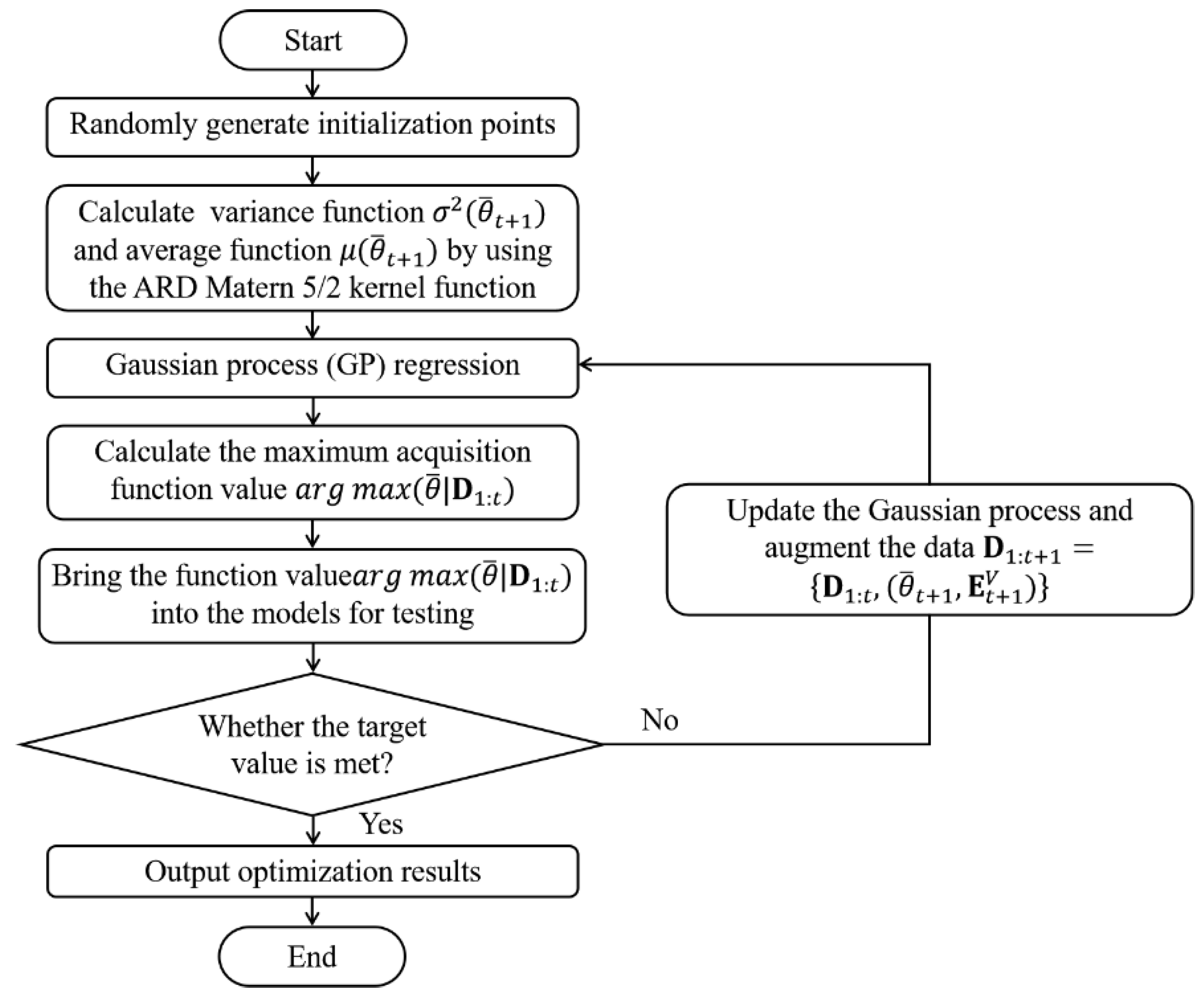
3.2. Bayesian Optimization

To improve the prediction performance of the model, this study uses Bayesian optimization to determine some important hyperparameters in random forest, isolation forest, and fully-connected ANN and CNN. The hyperparameters herein are the non-trainable parameters in the model. Those parameters (for example, the number of neurons and the structure of the network layer) are set before the training process starts. Nevertheless, a few hyperparameters, such as the number of trees and the number of predictor variables to sample at each node, are important hyperparameters in random forest and isolation forest. These parameters may have an important impact on the calculation performance of the forest [29]. Other parameters, such as the regularization coefficient and the learning rate, are important hyperparameters in neural networks. These parameters are very important for the neural network model to improve robustness to databases with small sample sizes.
Since Bayesian optimization has the advantage of sample efficiency, a relatively good hyperparameter combination can be found with a very small number of cycles. The calculation principle of adopting it to determine hyperparameters is as follows:
The basic assumption that the objective function E v ( θ ¯ ) is adopted for Bayesian optimization is obtained, a priori, by the Gaussian process (GP), E v ( θ ¯ ) ~ N ( 0 , K ) ;   θ ¯   is the hyperparameter vector considered in this study. Since E v ( θ ¯ ) is corrupted by Gaussian noise with a mean value of zero and a standard deviation of σ n o i s e , the kernel matrix can be expressed as [30]:
K = k ( θ ¯ 1 , θ ¯ 1 ) k ( θ ¯ 1 , θ ¯ t ) k ( θ ¯ t , θ ¯ 1 ) k ( θ ¯ 1 , θ ¯ t ) + σ n o i s e 2 I
where k ( θ ¯ t , θ ¯ t ) is the covariance function. The results of previous iterations are expressed as: D 1 : t = ( θ ¯ 1 : t , E 1 : t V ) , where E 1 : t V = E v ( θ ¯ 1 : t ) . Assume θ ¯ t + 1 as the next point to estimate and the value of the function at θ ¯ t + 1 as E t + 1 V = E v ( θ ¯ t + 1 ) . E 1 : t V and E t + 1 V are joint Gaussian expressions under GP prior. The predictive distribution can be obtained as follows [31]:
E t + 1 V | D 1 : t ~ N ( μ ( θ ¯ t + 1 ) , σ 2 ( θ ¯ t + 1 ) + σ n o i s e 2
where
μ ( θ ¯ t + 1 ) = k T ( K + σ n o i s e 2 I ) 1 E 1 : t V
σ 2 ( θ ¯ t + 1 ) = k ( θ ¯ t + 1 , θ ¯ t + 1 ) k T ( K + σ n o i s e 2 I ) 1 k
k = [ k ( θ ¯ t + 1 , θ ¯ 1 ) k ( θ ¯ t + 1 , θ ¯ 2 ) k ( θ ¯ t + 1 , θ ¯ t ) ] T
It can be seen from the above formulas, that both the predicted variance function σ 2 ( θ ¯ t + 1 ) and the predicted mean function μ ( θ ¯ t + 1 ) depend on the choice of the covariance function k ( θ ¯ t , θ ¯ t ) , and they jointly determine the choice of the covariance function E t + 1 V | D 1 : t .
This study uses the automatic relevance determination (ARD) Matérn 5/2 kernel [32]. This choice adapts to the problem of the ARD squared index kernel. It is impractical for such a covariance function to appear in the actual sample function optimization problem [33]. For t = 1 , 2 , N , the detailed calculation steps of the hyperparameter determination algorithm based on Bayesian optimization are shown in Figure 4 [34].

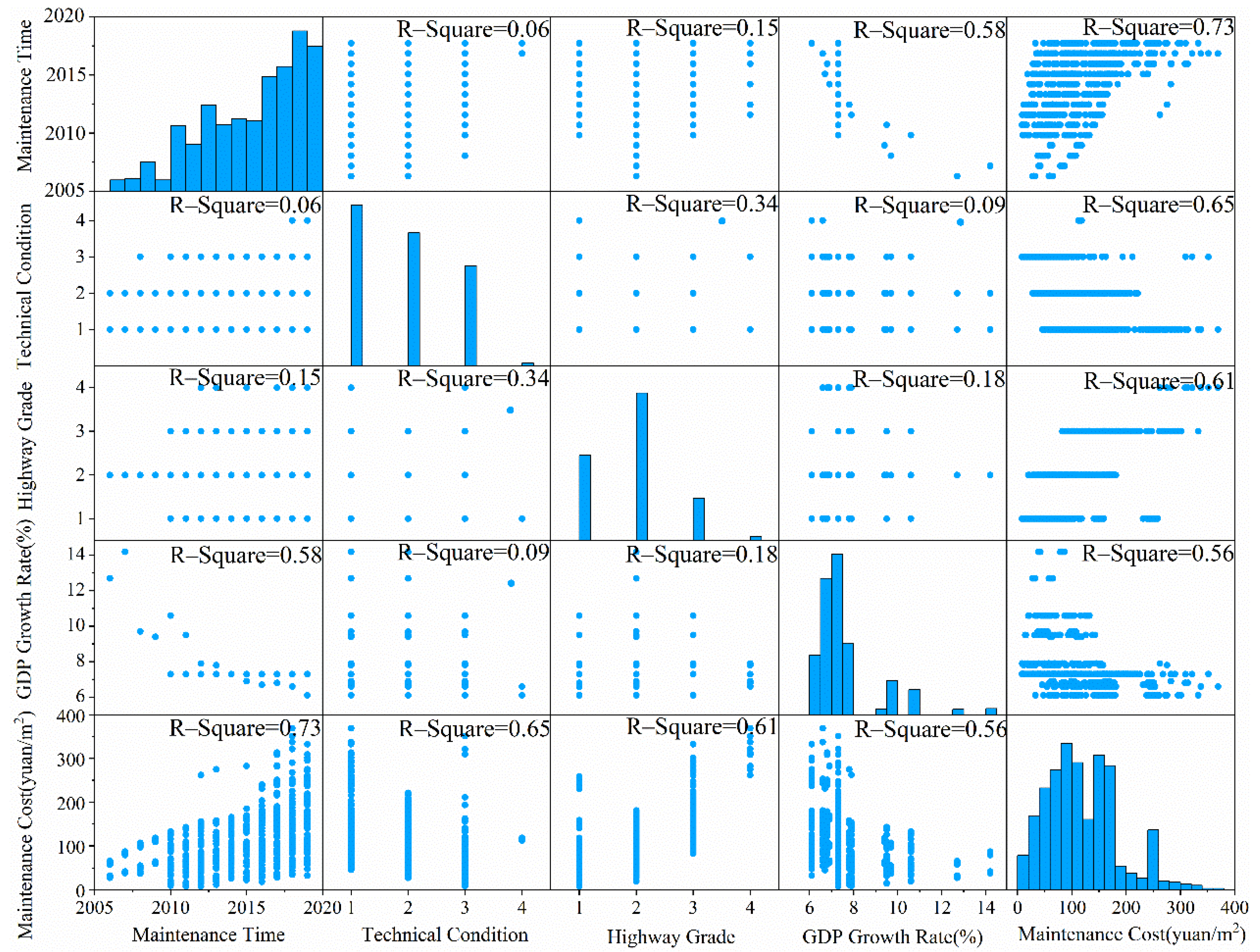
3.3. Exploratory Data Analysis

We performed an exploratory data analysis on bridge maintenance cost data to verify the effectiveness of the random forest method. Exploratory data analysis methods focus on the true distribution of data and emphasize the visualization of data. It can help users see the relationship between the data and the selected feature at a glance, so as to detect the validity of the feature [35]. EDA is different from the initial data analysis (IDA) in that it focuses more on checking the assumptions required for the model fit and hypothesis testing, deals with missing values, and performs variable transformations as needed [36].

3.4. Sample Screening

Anomaly detection is an important step in pre-processing the training data. The main function of anomaly detection is to check whether there are input errors and unreasonable data. Ignoring the existence of outliers in engineering practices is very dangerous. Incorporating outliers into the calculation and analysis processes of data without excluding them will adversely affect the training and prediction results. For the outlier detection of actual engineering data, scholars have carried out valuable research. For example, Xu et al. adopted wavelet transform and generalized Pareto distribution for data processing and proposed a two-level anomaly detection method, namely the threshold-based anomaly detection and anomaly trend detection [37]. Zhang et al. proposed an online detection method for structural health monitoring data anomalies based on the Bayesian dynamic linear model. This method has better calculation accuracy and higher calculation efficiency [38].
The isolation forest method was proposed by Zhou et al. in 2008 [39]. In 2011, the method was applied to the anomaly detection of data samples [40]. In isolated forests, anomalies are defined as points that are more sparsely distributed and further away from high-density groups. In the feature space constructed by the isolation forest, if the data distribution in a certain area is sparse, it means that the probability of normal data values appearing in that area is very low. Therefore, if a certain data frequently appears in these areas, it is judged as an anomaly. Isolation forest is an unsupervised anomaly detection method suitable for continuous numerical data. That is, it does not require labeled samples for training, and the method has good robustness to data with low feature dimensions. Taking into account the data characteristics of the bridge maintenance costs in this study, it was necessary to choose an anomaly detection method that was suitable for small datasets with low feature dimensions. The isolation forest method has been widely used in the detection of anomalies in actual engineering data. For example, smart grid data [41] and optical emission spectroscopy data [42]. The isolation forest method has been proven to process data quickly and efficiently. It is particularly suitable for small and medium datasets with low feature dimensions. Therefore, this study adopted it as a method of anomaly detection.
Consider a dataset X = { x 1 , x 2 , , x n } with n samples and d features. First, decision trees are built. Then, a feature q and its segmentation threshold p are selected randomly. Finally, the dataset X is segmented recursively until there is only one sample x i on the node. The length of the segmentation path of sample x i from the root node to the leaf node in the decision tree is represented by h ( x ) . For the dataset X, the average path length of the decision trees is:
c ( n ) = { 2 H ( n 1 ) 2 ( n 1 ) / n f o r   n > 2 1 f o r   n = 2 0 o t h e r w i s e
where n is the number of samples and H ( k ) is the harmonic number, which can be estimated by H ( k ) = ln k + ξ , where   ξ is Euler’s constant. As c ( n ) is the average of h ( x ) for the given n, we use it to normalize h ( x ) . The anomaly score s of an instance x is defined as:
s ( x , n ) = 2 E ( h ( x ) ) c ( n )
where E ( h ( x ) ) is the average value of h ( x ) is the average value of. The following conditions apply to the three special values of abnormal scores:
(a)
When E ( h ( x ) ) 0 ,   s 1 ;
(b)
When E ( h ( x ) ) n 1 ,   s 0 ;
(c)
When E ( h ( x ) ) c ( n ) ,   s 0.5 .
We can make the following assessment based on the anomaly score   s . If an instance returns a value of s that is very close to 1, then it is definitely an anomaly. If an instance has an s value much less than 0.5, then it can quite safely be regarded as a normal instance. If all instances return s 0.5 , then there are no significant anomalies for all data in this sample set.

3.5. The Fully-Connected ANN Model

The fully-connected ANN is an information system constructed by theoretically abstracting, simplifying, and simulating the structure, function, and basic characteristics of the real neural network in the human brain [43]. The BP neural network, currently the most widely used fully-connected ANN, is a multi-layer feedforward neural network trained according to the error backpropagation algorithm. The transfer function used by the neurons of the BP neural network is usually a differentiable function that can realize any nonlinear mapping between the input and the output. Therefore, the BP neural network has a wide range of applications in pattern recognition, risk evaluation, intelligent prediction, etc. [44].
The BP neural network has arbitrarily complex pattern classification capabilities and excellent multi-dimensional function mapping capabilities. The objective function of it is the square of the network error; the minimum value of the objective function is calculated through the gradient descent method [45]. The detailed calculation process is as follows:
(1)
The connection weight value and threshold are initialized based on random values.
(2)
The output of each unit of the hidden layer and the output layer is calculated according to the parameters selected by the input mode and output mode. In this study, the ReLU [46] is used as the activation function of the hidden layer. The Tanh [47] is used as the activation function of the output layer.
The ReLU can be defined as
f ( x ) = max ( 0 , x )
The Tanh can be defined as
f ( x ) = e x e x e x + e x
(3)
The new connection weights and thresholds are calculated using the Equations (13)–(16). The modification of the neuron threshold:
θ k ( t + 1 ) = θ k ( t ) + η t σ k , ( t = 1 , 2 , , p ; k = 1 , 2 , , l )
θ j ( t + 1 ) = θ j ( t ) + η t σ j , ( t = 1 , 2 , , p ; j = 1 , 2 , , m )
where θ j and θ k are the threshold values of the j-th node in the hidden layer and the k-th node in the output layer, respectively ;   σ j and σ k are errors of the j-th node in the hidden layer and the k-th node in the output layer respectively.   η t is the learning rate of the t-th training iteration.
The update formula of the weight is as follows:
ω j k ( t + 1 ) = ω j k ( t ) + Δ ω j k ( t ) , ( t = 1 , 2 , , p )
ν i j ( t + 1 ) = ν i j ( t ) + Δ ν i j ( t ) , ( t = 1 , 2 , , p )
where t is the number of iterations in the training process; ν i j is the weight value updating from the input layer to the hidden layer; ω j k is the weight value updating from the hidden layer to the output layer.
(4)
Return to the second step to train the neural network and update the learning input mode continuously until the number of training times reaches the preset value. The basic flow of the above calculation process is shown in Figure 5:
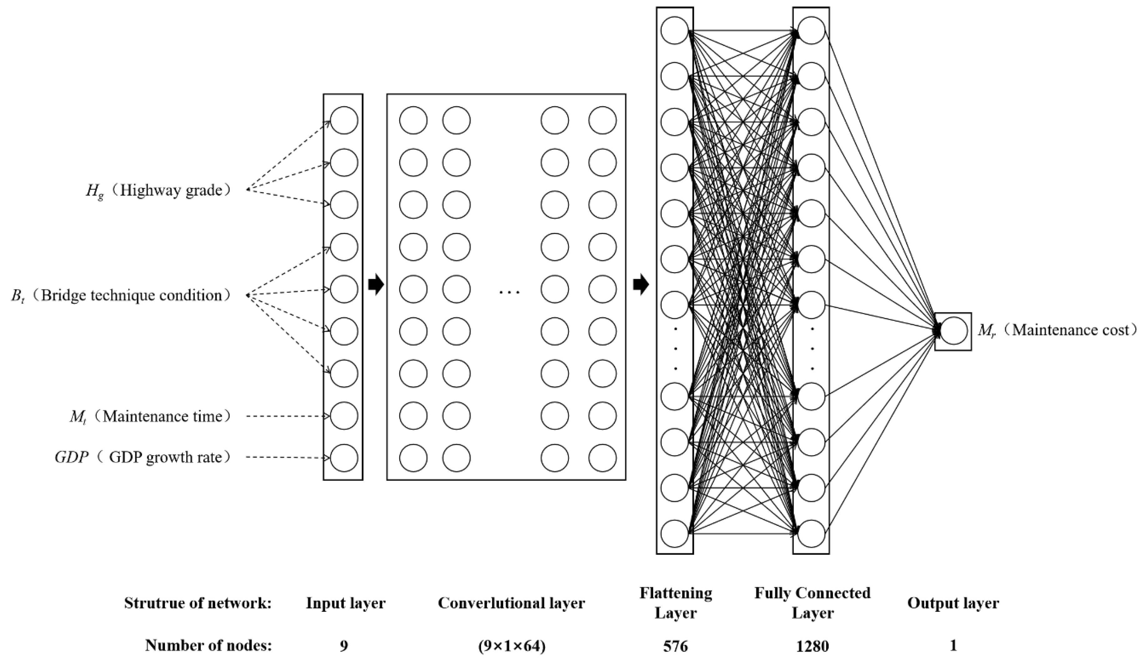
3.6. CNN Model

CNN is currently one of the most widely used deep learning algorithms. Compared to the fully-connected ANN, the most important features of CNN are local perception and parameter sharing [48]. The main parts of a CNN are the convolutional layer, pooling layer, and activation function [49]. CNN reduces the complexity of the network model through three strategies: a local receptive field, weight sharing, and downsampling. They are widely used in the fields of image classification, speech recognition, and intelligent prediction [50].
CNN has proven to be a reliable technique for extracting hidden features because it can complete the automatic creation of filters [51]. By using the convolution filter to act on all the feature spaces of the input data, for each perception area, the data at the corresponding position are multiplied by the weight in the convolution filter, and then summed as the input of the next layer of neurons. In the same convolution layer of CNN, all neurons are set to have no connection and only the weight of the filter is shared. Therefore, CNN is more effective than multi-layer perceptron training with the same structure. Each convolution layer can be expressed as [52]:
y i = f ( i = 1 n W i x i + b )
where y i indicates the results after convolution, f denotes the activation function, W i indicates the weights of the convolution filter, b indicates the bias terms.
The CNN model was built based on Python and TensorFlow in this study. On the basis of the aforementioned fully-connected ANN model, a convolution operation was added, and the other parts were similar to the fully-connected ANN model. The CNN consisted of an input layer, a convolutional layer, a flattening layer, a fully connected layer, and an output layer. The convolution kernel size was 2 × 1, the channels of the convolutional layer were 64. After convolution, the number of nodes changed from 9 to 576, realizing the deep extraction of features. In view of the few input parameters of this model, pooling operation was not performed.
ReLU was used as the activation function of the convolutional layer and the fully connected layer. Tanh was used as the activation function of the output layer. Adam [53] was the optimization algorithm in this study.
Adam can be defined as
m t = μ × m t 1 + ( 1 μ ) × g t
n t = ν × n t 1 + ( 1 ν ) × g t 2
m t ^ = m t 1 μ t
n t ^ = n t 1 ν t
θ t = m t ^ n t ^ + ϵ × η
where μ , ν indicate the exponential decay rates for the moment estimates, g t indicates the gradients of stochastic objectives at timestep t, m t indicates the biased first moment estimation of gradients, n t indicates the second raw moment estimation of gradients, m t ^ and n t ^ respectively, indicate the unbiased estimate after correcting m t and n t , θ t indicates the result parameter. After Bayesian optimization, the hyperparameters in the neural network are η = 0.001 , μ = 0.9 , ν = 0.999 and ϵ = 10 8 . The basic flow of the above calculation process is shown in Figure 6:

4. Implementation Results of a Fully-Connected ANN and CNN

4.1. Influencing Factors of Bridge Maintenance Costs

The random forest method in Section 3.1 was used to calculate the VIM values of eight influencing factors (GDP growth rate, maintenance time, bridge grade, bridge technical condition, bridge location, bridge age, superstructure, and highway grade). The calculation results are shown in Figure 7.
It can be seen from Figure 7 that the importance values of the four indicators of maintenance time, technical conditions, highway class, and GDP growth rate are all greater than 0.2. The importance of these four indicators is significantly higher than the other indicators, and the importance value of the other indicators is less than 0.1. Therefore, we select GDP growth rate, bridge technical conditions, highway grade, and maintenance time as the input parameters of the prediction models.
The scatter graph matrix was adopted to conduct an exploratory data analysis on the database, to test the correlation between the four input parameters selected in the previous section and bridge maintenance costs. The probability histogram is on the diagonal line of the matrix, which represents the frequency of occurrence of a corresponding label for a certain feature. The scatter diagram is on the non-diagonal line of the matrix, which represents the correlation between labels, corresponding to different maintenance cost characteristics.
A total of five characteristics of the four selected indicators, plus maintenance costs, were involved in the exploratory data analysis. Thus, the matrix consists of 5 probability histograms and 20 scatter plots. As can be seen from Figure 8, there is a certain correlation between the selected indicators and maintenance costs, while ensuring certain independence.

4.2. Sample Classification Based on Selected Indicators

All samples are classified according to four input indicators, as shown in Figure 9. The samples only contain three indicators: maintenance time, bridge technical condition, and highway grade.
In Figure 9, the maintenance cost samples are divided into three categories according to the highway grade. According to the technical conditions of the bridge, each category was divided into four sub-categories and the samples were sorted by maintenance time. The sample values increased significantly as the technical conditions of the bridge worsened. As the highway grade worsened, the sample values also tended to increase, and they gradually increased with maintenance time. These results demonstrate the feasibility of predicting the maintenance costs based on the classification of these indicators.

4.3. Sample Screening Based on Isolation Forest

Twenty-seven maintenance samples (6.8% of the total) were identified as outliers by the isolation forest method. We replaced the outliers with the average of the same type of data to ensure that the prediction accuracy improved without reducing the sample size. The sample distribution after replacement is shown in Figure 10.

4.4. Structure of the Sample Database

The constructed database contained a total of 399 maintenance cost samples. All samples were classified according to the highway grade and bridge technical condition. The 80% of samples with the earliest maintenance times in each type of data were selected into the training set for training. The 20% of samples with the latest maintenance times constituted the prediction set as the verification of the calculation results. A total of 320 samples were selected into the training set and 79 samples were selected into the prediction set. The detailed classification of the database is shown in Table 4.

4.5. Topology of the Fully-Connected ANN Model and CNN Model

In this study, a fully-connected ANN model was designed for maintenance cost prediction. It contained three layers: an input layer, a fully connected hidden layer, and an output layer. There are 9 neurons in the input layer, 980 neurons in the hidden layer, and 1 neuron in the output layer. The topology of the proposed model is shown in Figure 11.
It can be seen from Figure 12 that the output of the convolutional layer is a 9 × 64 matrix. The third layer is a flattening layer containing 576 neurons. The fourth layer is a fully connected layer containing 1280 neurons, and the final layer is the output layer.

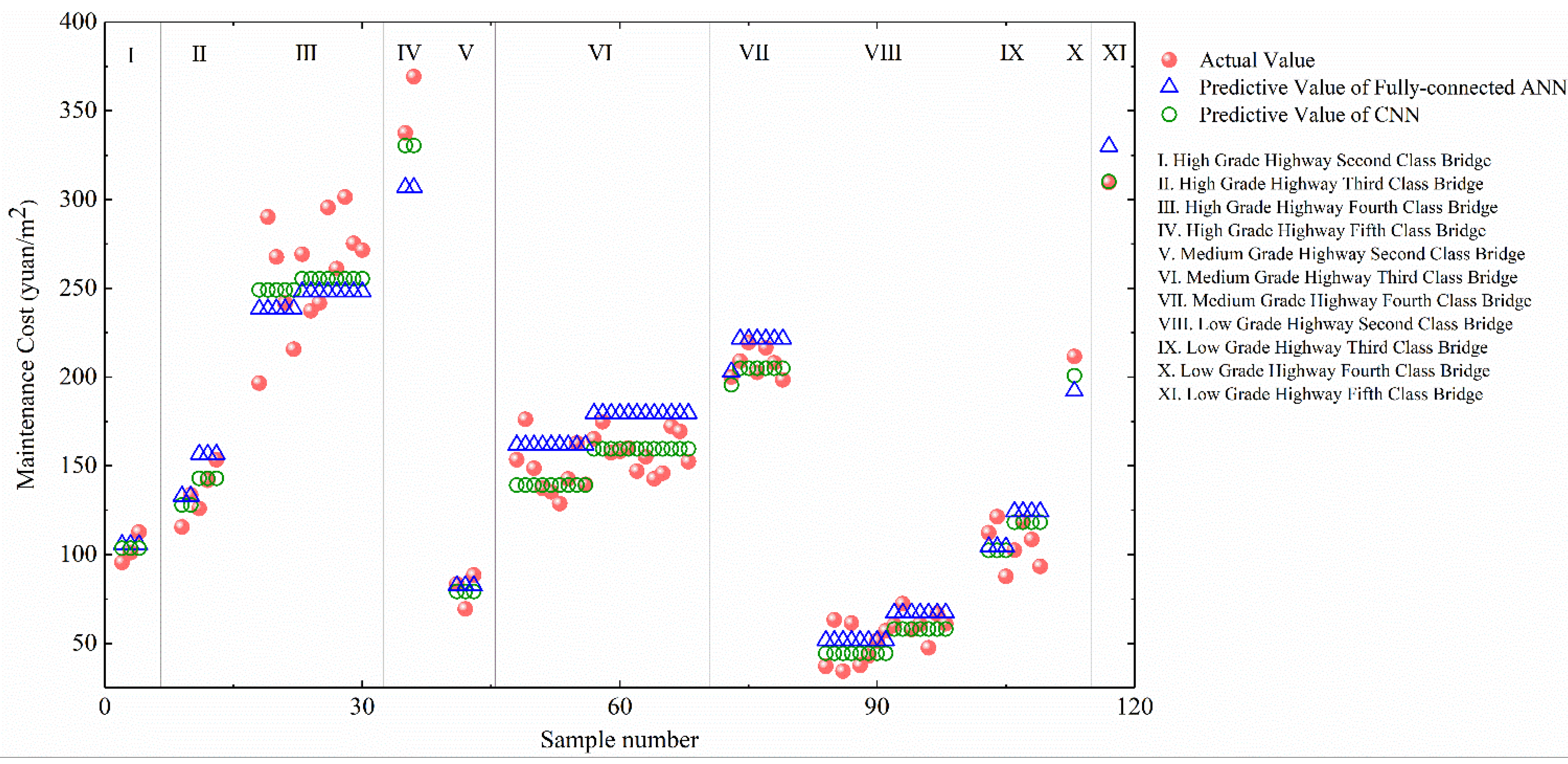
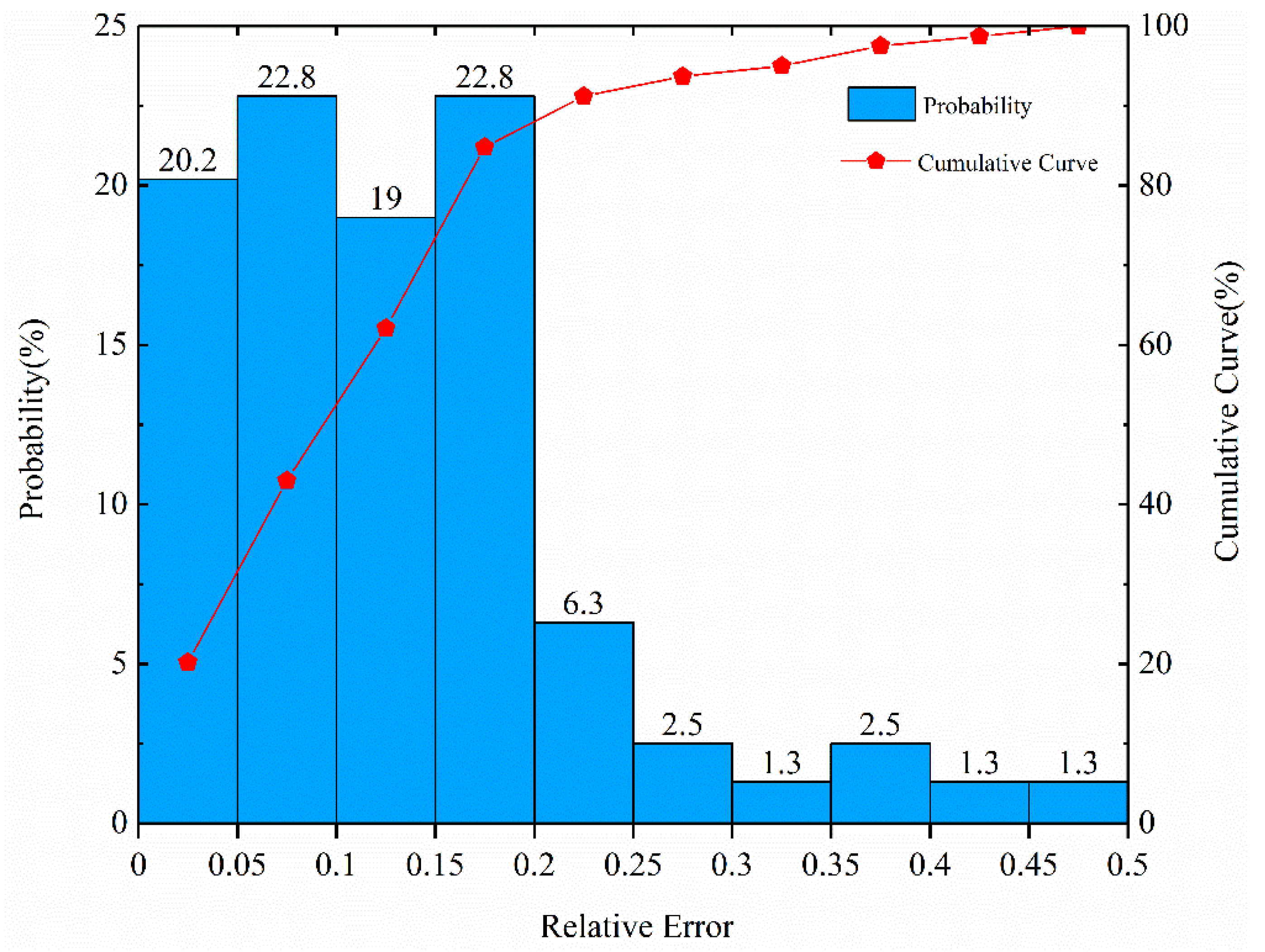
4.6. Accuracy Analysis of Prediction Model

The established fully-connected ANN model and CNN model were used to predict the cost of bridge maintenance in the future. To verify the prediction accuracy of the model, the prediction result of the model was compared to the actual bridge maintenance costs. Figure 13 shows a comparison between the predicted values given by the two prediction models and the actual maintenance costs under the corresponding indicators.
The relative error distribution of the fully-connected ANN model is shown in Figure 14. It can be seen from Figure 14 that the relative error is less than 20% for 84.8% of the prediction data and less than 30% for 93.6% of the prediction data.
The relative error distribution of the CNN model is shown in Figure 15. It can be seen from Figure 15 that 87.4% of the prediction results have a relative error of less than 20% and less than 30% for 98.7% of the prediction data.
To compare the predictive performance of the two models, a linear regression model was added as a baseline for comparison. Linear, quadratic, and exponential curve fitting equations can be established based on regression analysis. Finally, the quadratic curve with the highest average goodness of fit (R2) was selected as the fitting form, a prediction model was established, and the regression coefficient was calculated. The regression analysis model form is defined as follows:
y = a t 2 + b t + c
where y indicates the maintenance costs for the bridge; a, b, and c are parameters for regression analysis; t indicates time.
The relevant prediction error indicators for the fully-connected ANN model, the CNN model, and regression model are presented in Table 5.
It is apparent—from the prediction results and error analyses of the two models—that the CNN model provides better predictions of the bridge maintenance costs than the fully-connected ANN. Through the convolution operation, multi-dimensional feature extraction can be applied to each maintenance cost indicator, improving the prediction accuracy.

5. Conclusions

This paper established a sample database of bridge maintenance costs over the period 2010–2019, based on the actual engineering data of 268 bridges in coastal and inland areas of China. Two bridge maintenance cost prediction models were developed based on fully-connected ANN and CNN approaches, respectively, and their prediction results were compared. The conclusions of this study are as follows:
(1) The eight main factors of bridge maintenance costs were evaluated based on the random forest method. The VIM of four indicators (technical condition, maintenance time, GDP growth rate, and highway grade) were greater than 0.2. The VIM values of the bridge age, superstructure, bridge grade, and bridge location were all less than 0.1.
(2) An outlier detection method based on the isolation forest method was adopted to identify maintenance cost samples that were significantly different from the bridge maintenance costs. As a result, 27 maintenance samples, accounting for 6.8% of the total, were identified as outliers and replaced by the average values of similar data.
(3) Prediction models were established based on fully-connected ANN and CNN, respectively. The mean absolute error, root mean square error, average relative error, and mean absolute percent error of the fully-connected ANN model were 17.4 Yuan/m2, 21.2 Yuan/m2, 13.02%, and 12.59% respectively. The mean absolute error, root mean square error, average relative error, and mean absolute percent error of the CNN model were 12.5 Yuan/m2, 16.7 Yuan/m2, 9.45%, and 9.35%, respectively. It can be concluded from the comparative analysis that the prediction accuracy of the CNN model is higher than that of the fully-connected ANN model.

6. Prospect

There are several limitations in this paper, which could guide the directions of future studies. The sample size of the database was limited, and the coverage was not wide enough. As a result, indicators, such as geological conditions and extreme weather conditions, were not fully considered. A more comprehensive bridge maintenance cost database is needed to support future studies. Social and economic development is a relatively broad concept and a complex economic problem. How to quantify and find the relationship between it and bridge maintenance costs is a topic worthy of in-depth study. This study used GDP growth rate as an indicator of social and economic development (and achieved good results). Further research could explore other economic indicators to quantify this impact based on an in-depth analysis of the correlation between economic development and bridge maintenance costs.

Author Contributions

Writing original draft preparation, C.W.; data curation, C.Y.; software, S.Z. (Siguang Zhao); visualization, S.Z. (Shida Zhao); writing review and editing, Y.L. All authors have read and agreed to the published version of the manuscript.

Funding

This research was funded by [China Railway Major Bridge Reconnaissance and Design Institute Co., Ltd.] grant number [2016YFC0802202-2].

Data Availability Statement

To promote the further study of the bridge maintenance cost prediction, the original data used in this study were uploaded to the public database under the premise of not disclosing the specific name and address of the bridge, after the consent of all original data providers. The link to obtain the data is as follows: https://figshare.com/s/53131800943d092a4b49 (accessed on 15 February 2022).

Acknowledgments

The writers acknowledge partial financial support from the China Railway Major Bridge Reconnaissance & Design Institute Co., Ltd., through grant no. 2016YFC0802202-2. The writers thank the Foshan Transportation Bureau, the Sichuan Communication Surveying & Design Institute, the Deyang Transportation Bureau, and other departments for providing raw data of the bridge maintenance costs.

Conflicts of Interest

The authors declare no conflict of interest. The contents of this paper reflect the views of the writers and not necessarily the views of Southwest Jiaotong University. The writers are responsible for the facts and the accuracy of the data presented in this paper. The contents do not necessarily reflect the official views or policies of either the Foshan Transportation Bureau or the Deyang Transportation Bureau at the time of publication.

References

  1. American Society of Civil Engineers. Report Card for America’s Infrastructure; ASCE: Reston, VA, USA, 2021; Available online: https://www.asce.org/ (accessed on 26 February 2022).
  2. Cadenazzi, T.; Dotelli, G.; Rossini, M.; Nolan, S.; Nanni, A. Cost and environmental analyses of reinforcement alternatives for a concrete bridge. Struct. Infrastruct. Eng. 2020, 16, 787–802. [Google Scholar] [CrossRef]
  3. Zhou, J.; Zheng, D. Strategic Thinking on Safeguarding Bridge Safety in China. China Eng. Sci. 2017, 19, 27–37. [Google Scholar] [CrossRef]
  4. MOT—Ministry of Transport of the People’s Republic of China. Statistical Bulletin on the Development of the Transportation Industry; Ministry of Transport of the People’s Republic of China: Beijing, China, 2020. Available online: http://www.gov.cn/xinwen/2021-05/19/content_5608523.htm (accessed on 26 February 2022).
  5. Wang, Z.F.; Dai, G.H. Maintenance Strategies of Historical Bridges in China. Appl. Mech. Mater. 2012, 178–181, 2264–2267. [Google Scholar] [CrossRef]
  6. Barone, G.; Frangopol, D.; Soliman, M. Optimization of Life-Cycle Maintenance of Deteriorating Bridges with Respect to Expected Annual System Failure Rate and Expected Cumulative Cost. J. Struct. Eng. 2014, 140, 04013043. [Google Scholar] [CrossRef] [Green Version]
  7. Sabatino, S.; Frangopol, D.M.; Dong, Y. Sustainability-informed maintenance optimization of highway bridges considering multi-attribute utility and risk attitude. Eng. Struct. 2015, 102, 310–321. [Google Scholar] [CrossRef]
  8. Ghodoosi, F.; Abu-Samra, S.; Zeynalian, M.; Zayed, T. Maintenance Cost Optimization for Bridge Structures Using System Reliability Analysis and Genetic Algorithms. J. Constr. Eng. Manag. 2018, 144, 04017116. [Google Scholar] [CrossRef]
  9. Lee, J.H.; Choi, Y.; Ann, H.; Jin, S.Y.; Lee, S.-J.; Kong, J.S. Maintenance Cost Estimation in PSCI Girder Bridges Using Updating Probabilistic Deterioration Model. Sustainability 2019, 11, 6593. [Google Scholar] [CrossRef] [Green Version]
  10. Li, Z.; Kaul, H.; Kapoor, S.; Veliou, E.; Zhou, B.; Lee, S. New Methodology for Transportation Investment Decisions with Consideration of Project Interdependencies. Transp. Res. Rec. 2012, 2285, 36–46. [Google Scholar] [CrossRef]
  11. Shi, X.; Zhao, B.; Yao, Y.; Wang, F. Prediction Methods for Routine Maintenance Costs of a Reinforced Concrete Beam Bridge Based on Panel Data. Adv. Civ. Eng. 2019, 2019, 5409802. [Google Scholar] [CrossRef] [Green Version]
  12. Miyamoto, A.; Kawamura, K.; Nakamura, H. Bridge Management System and Maintenance Optimization for Existing Bridges. Comput. Aided Civ. Infrastruct. Eng. 2000, 15, 45–55. [Google Scholar] [CrossRef]
  13. Mohammad, B.S.; Yasser, M.; Maria, A.H. Prediction of maintenance cost for road construction equipment: A case study. Can. J. Civ. Eng. 2016, 43, 125–136. [Google Scholar]
  14. Echaveguren, T.; De Concepción, U.; Dechent, P. Allocation of bridge maintenance costs based on prioritization indexes. Rev. Construcción 2019, 18, 568–578. [Google Scholar] [CrossRef]
  15. Yong, H.Y.; Yuan, H.J.; Xuan, C.W. Pavement Performance Prediction Methods and Maintenance Cost Based on the Structure Load. Procedia Eng. 2016, 137, 41–48. [Google Scholar] [CrossRef] [Green Version]
  16. Zhu, J.-S.; Huang, F.-M.; Guo, T.; Song, Y.-H. Residual life evaluation of prestressed reinforced concrete highway bridges under coupled corrosion-fatigue actions. Adv. Steel Constr. 2015, 11, 372–382. [Google Scholar] [CrossRef] [Green Version]
  17. Testa, R.B.; Yanev, B.S. Bridge maintenance level assessment. Comput. Aided Civ. Infrastruct. Eng. 2002, 17, 358–367. [Google Scholar] [CrossRef]
  18. JTG B01-2014; Technical Standard of Highway Engineering. China Communications Press Co., Ltd.: Beijing, China, 2019.
  19. JTG 5210-2018; Highway Performance Assessment Standards. China Communications Press Co., Ltd.: Beijing, China, 2018.
  20. JTG D60-2015; General Specifications for Design of Highway Bridges and Culverts. China Communications Press Co., Ltd.: Beijing, China, 2015.
  21. Bacha, E.L. A three-gap model of foreign transfers and the GDP growth rate in developing countries. J. Dev. Econ. 1990, 32, 279–296. [Google Scholar] [CrossRef] [Green Version]
  22. Jiang, Y.; Guo, Y.; Zhang, Y. Forecasting China’s GDP growth using dynamic factors and mixed-frequency data. Econ. Model. 2017, 66, 132–138. [Google Scholar] [CrossRef]
  23. NBS—National Bureau of Statistics of China. China Statistical Yearbook; National Bureau of Statistics of China: Beijing, China, 2020. Available online: http://www.stats.gov.cn/tjsj/ndsj/ (accessed on 26 February 2022).
  24. Hinton, G.; Deng, L.; Yu, D.; Dahl, G.E.; Kingsbury, B. Deep Neural Networks for Acoustic Modeling in Speech Recognition: The Shared Views of Four Research Groups. IEEE Signal Processing Mag. 2012, 29, 82–97. [Google Scholar] [CrossRef]
  25. Sun, D.; Wen, H.; Wang, D.; Xu, J. A random forest model of landslide susceptibility mapping based on hyperparameter optimization using Bayes algorithm. Geomorphology 2020, 362, 107201. [Google Scholar] [CrossRef]
  26. Tang, Z.; Mei, Z.; Liu, W.; Xia, Y. Identification of the key factors affecting Chinese carbon intensity and their historical trends using random forest algorithm. J. Geogr. Sci. 2020, 30, 743–756. [Google Scholar] [CrossRef]
  27. Richard, C.D.; Edwards, T.C., Jr.; Beard, K.H.; Cutler, A.; Hess, K.T.; Gibson, J.; Lawler, J.J. Random forests for classification in ecology. Ecology 2007, 88, 2783–2792. [Google Scholar]
  28. Liaw, A.; Wiener, M. Classification and Regression by Random Forest. R News 2002, 2, 18–22. Available online: https://www.researchgate.net/publication/228451484 (accessed on 26 February 2022).
  29. Mostafaei, M.; Javadikia, H.; Naderloo, L. Modeling the effects of ultrasound power and reactor dimension on the biodiesel production yield: Comparison of prediction abilities between response surface methodology (RSM) and adaptive neuro-fuzzy inference system (ANFIS). Energy 2016, 115, 626–636. [Google Scholar] [CrossRef]
  30. Mathern, A.; Steinholtz, O.S.; Sjöberg, A.; Önnheim, M.; Ek, K.; Rempling, R.; Gustavsson, E.; Jirstrand, M. Multi-objective constrained Bayesian optimization for structural design. Struct. Multidiscip. Optim. 2020, 63, 689–701. [Google Scholar] [CrossRef]
  31. Rasmussen, C.E.; Edward, C.; Nickisch, H. Gaussian Processes for Machine Learning (GPML) Toolbox. J. Mach. Learn. Res. 2010, 11, 3011–3015. [Google Scholar]
  32. Calandra, R.; Gopalan, N.; Seyfarth, A.; Peters, J.; Deisenroth, M.P. Bayesian Gait Optimization for Bipedal Locomotion, International Conference on Learning and Intelligent Optimization; Springer: Lake Tahoe, NV, USA, 2014; Available online: https://0-link-springer-com.brum.beds.ac.uk/chapter/10.1007/978-3-319-09584-4_25 (accessed on 26 February 2022).
  33. Liang, X. Image-based post disaster inspection of reinforced concrete bridge systems using deep learning with Bayesian optimization. Comput.-Aided Civ. Infrastruct. Eng. 2019, 34, 415–430. [Google Scholar] [CrossRef]
  34. Zhang, Y.-M.; Wang, H.; Mao, J.-X.; Xu, Z.-D.; Zhang, Y.-F. Probabilistic Framework with Bayesian Optimization for Predicting Typhoon-Induced Dynamic Responses of a Long-Span Bridge. J. Struct. Eng. 2021, 147, 04020297. [Google Scholar] [CrossRef]
  35. Urminder, S.; Manhoi, H.; Karin, D.; Syrkin, W.E. MetaOmGraph: A workbench for interactive exploratory data analysis of large expression datasets. Nucleic Acids Res. 2020, 48, e23. [Google Scholar]
  36. Xiao, C.; Ye, J.; Esteves, R.M.; Rong, C. Using Spearman’s correlation coefficients for exploratory data analysis on big dataset. Concurr. Comput. Pract. Exp. 2016, 28, 3866–3878. [Google Scholar] [CrossRef]
  37. Xu, X.; Ren, Y.; Huang, Q.; Fan, Z.-Y.; Tong, Z.-J.; Chang, W.-J.; Liu, B. Anomaly detection for large span bridges during operational phase using structural health monitoring data. Smart Mater. Struct. 2020, 29, 045029. [Google Scholar] [CrossRef]
  38. Zhang, Y.-M.; Wang, H.; Wan, H.-P.; Mao, J.-X.; Xu, Y.-C. Anomaly detection of structural health monitoring data using the maximum likelihood estimation-based Bayesian dynamic linear model. Struct. Health Monit. 2020, 20, 2936–2952. [Google Scholar] [CrossRef]
  39. Zhou, Z.-H.; Liu, F.T.; Ting, K.M. Isolation forest. In Proceedings of the 2008 Eighth IEEE International Conference on Data Mining, Pisa, Italy, 15–19 December 2008; pp. 413–422. Available online: https://0-ieeexplore-ieee-org.brum.beds.ac.uk/stamp/stamp.jsp?tp=&arnumber=4781136 (accessed on 26 February 2022).
  40. Liu, F.T.; Ting, K.M.; Zhou, Z.H. Isolation-Based Anomaly Detection. ACM Trans. Knowl. Discov. Data 2012, 6, 1–39. [Google Scholar] [CrossRef]
  41. Ahmed, S.; Lee, Y.; Hyun, S.-H.; Koo, I. Unsupervised Machine Learning-Based Detection of Covert Data Integrity Assault in Smart Grid Networks Utilizing Isolation Forest. IEEE Trans. Inf. Forensics Secur. 2019, 14, 2765–2777. [Google Scholar] [CrossRef]
  42. Puggini, L.; McLoone, S. An enhanced variable selection and Isolation Forest based methodology for anomaly detection with OES data. Eng. Appl. Artif. Intell. 2018, 67, 126–135. [Google Scholar] [CrossRef] [Green Version]
  43. Yao, X. Evolving artificial neural networks. Proc. IEEE 1999, 87, 1423–1447. [Google Scholar]
  44. Ding, S.; Su, C.; Yu, J. An optimizing BP neural network algorithm based on genetic algorithm. Artif. Intell. Rev. 2011, 36, 153–162. [Google Scholar] [CrossRef]
  45. Xiao, Z.; Ye, S.-J.; Zhong, B.; Sun, C.-X. BP neural network with rough set for short term load forecasting. Expert Syst. Appl. 2009, 36, 273–279. [Google Scholar] [CrossRef]
  46. Glorot, X.; Bordes, A.; Bengio, Y. Deep Sparse Rectifier Neural Networks. J. Mach. Learn. Res. 2011, 15, 315–323. [Google Scholar]
  47. Malfliet, W. The tanh method: A tool for solving certain classes of non-linear PDEs. Math. Methods Appl. Sci. 2005, 28, 2031–2035. [Google Scholar] [CrossRef]
  48. Liang, F.; Shen, C.; Wu, F. An iterative BP-CNN architecture for channel decoding. IEEE J. Sel. Top. Signal Processing 2018, 12, 144–159. [Google Scholar] [CrossRef] [Green Version]
  49. Lawrence, S.; Giles, C.L.; Tsoi, A.C.; Back, A.D. Face recognition: A convolutional neural-network approach. IEEE Trans. Neural Netw. 1997, 8, 98–113. [Google Scholar] [CrossRef] [PubMed] [Green Version]
  50. Janssens, O.; Slavkovikj, V.; Vervisch, B.; Stockman, K.; Loccufier, M.; Verstockt, S.; Van de Walle, R.; Van Hoecke, S. Convolutional Neural Network Based Fault Detection for Rotating Machinery. J. Sound Vib. 2016, 377, 331–345. [Google Scholar] [CrossRef]
  51. Oehmcke, S.; Zielinski, O.; Kramer, O. Input quality aware convolutional LSTM networks for virtual marine sensors. Neurocomputing 2018, 275, 2603–2615. [Google Scholar] [CrossRef]
  52. Ding, L.; Fang, W.; Luo, H.; Love, P.E.D.; Zhong, B.; Ouyang, X. A deep hybrid learning model to detect unsafe behavior: Integrating convolution neural networks and long short-term memory. Autom. Constr. 2018, 86, 118–124. [Google Scholar] [CrossRef]
  53. Kingma, D.; Ba, J. Adam: A Method for Stochastic Optimization. Comput. Sci. 2014. [Google Scholar] [CrossRef]
Figure 1. The classification of bridge maintenance cost samples; (a) bridge grade; (b) superstructure; (c) bridge technical condition; (d) highway grade; (e) bridge age; (f) bridge location; (g) maintenance time.
Applsci 12 03595 g001aApplsci 12 03595 g001b
Figure 2. GDP growth rate in China.
Applsci 12 03595 g002
Figure 3. A comparative study of a fully-connected ANN and CNN implementation framework.
Applsci 12 03595 g003
Figure 4. Flow chart for Bayesian optimization calculation.
Applsci 12 03595 g004
Figure 5. The calculation process chart for the fully-connected ANN model.
Applsci 12 03595 g005
Figure 6. The calculation process chart for the CNN model.
Applsci 12 03595 g006
Figure 7. The calculation results of VIM of the main influencing factors.
Applsci 12 03595 g007
Figure 8. Scatterplot matrix for selected indicators.
Applsci 12 03595 g008
Figure 9. Sample classification chart.
Applsci 12 03595 g009
Figure 10. Sample classification diagram after data screening and replacement.
Applsci 12 03595 g010
Figure 11. Topology of the fully-connected ANN prediction model.
Applsci 12 03595 g011
Figure 12. Topology of the CNN prediction model.
Applsci 12 03595 g012
Figure 13. Comparison of actual maintenance costs and predicted results given by the fully-connected ANN model and the CNN model.
Applsci 12 03595 g013
Figure 14. Relative error distribution of fully-connected ANN prediction model.
Applsci 12 03595 g014
Figure 15. Relative error distribution of CNN prediction model.
Applsci 12 03595 g015
Table 1. Standards for dividing highway grade indicators.
Highway GradeHighway Traffic GradeDesign Service Life
HighExpressway,
First class highway
20 years
Medium Second class highway15 years
Low Third class highway,
Fourth class highway
10 years
Table 2. Indicators classification of bridge technical conditions.
Weighted Mark for Overall Technical Condition of BridgesBridge Technical Condition Grade Dj
First Class BridgeSecond Class BridgeThird Class BridgeFourth Class BridgeFifth Class Bridge
Dr(95,100)(80,95)(60,80)(40,60)(0,40)
Table 3. Indicators classification of bridge grade indicators.
Extra-Large BridgeLarge BridgeMedium BridgeSmall Bridge
Full length (m)(1000,+∞)(100,1000)(30,100)(8,30)
Single span (m)(150,+∞)(40,150)(20,40)(5,20)
Table 4. Classification of the database.
Highway GradeBridge CategoryTraining SetPrediction Set
HighSecond143
Third235
Fourth5413
MediumSecond52
Third113
Fourth8421
Fifth277
LowSecond6416
Third307
Fourth61
Fifth21
Total 32079
Table 5. Relevant error indicators of the fully-connected ANN model, CNN model prediction, and regression model.
Prediction ModelMean Absolute Error
(Yuan/m2)
Maximum Error (Yuan/m2)Minimum Error (Yuan/m2)Root Mean Square Error
(Yuan/m2)
ANN16.859.40.219.7
CNN12.552.60.316.7
Regression model20.657.83.621.9
Prediction ModelAverage Relative Error (%)Maximum Relative Error (%)Minimum Relative Error (%)Mean Absolute Percent Error (%)
ANN12.05%52.71%0.28%11.89%
CNN9.45%29.83%0.24%9.35%
Regression model15.95%46.51%3.15%15.22%
Publisher’s Note: MDPI stays neutral with regard to jurisdictional claims in published maps and institutional affiliations.

