
An Improved Shoulder Line Extraction Method Fusing Edge Detection and Regional Growing Algorithm

1
School of Geography, Nanjing Normal University, Nanjing 210023, China
2
Key Laboratory of Virtual Geographic Environment, Nanjing Normal University, Ministry of Education, Nanjing 210023, China
3
Jiangsu Center for Collaborative Innovation in Geographical Information Resource Development and Application, Nanjing 210023, China
*
Author to whom correspondence should be addressed.
Appl. Sci. 2022, 12(24), 12662; https://0-doi-org.brum.beds.ac.uk/10.3390/app122412662
Submission received: 26 October 2022
/
Revised: 2 December 2022
/
Accepted: 7 December 2022
/
Published: 10 December 2022
(This article belongs to the Special Issue Remote Sensing Applications in Archaeology, Geography, and the Earth Sciences)
Abstract
:Shoulder lines can best depict the morphological characteristics of the Loess Plateau. Moreover, a shoulder line depicts the external appearance of spatial differentiation of loess landforms and the internal mechanism of loess landform evolution. The efficient and accurate extraction of shoulder lines can help to deepen the re-understanding of the morphological structure and differentiation of loess landforms. However, the problem of shoulder line continuity in the extraction process has not been effectively solved. Therefore, based on high-resolution satellite images and digital elevation model (DEM) data, this study introduced the regional growing algorithm to further correct edge detection results, thereby achieving complementary advantages and improving the accuracy and continuity of shoulder line extraction. First, based on satellite images, the edge detection method was used to extract the original shoulder lines. Subsequently, by introducing the regional growing algorithm, the peaks and the outlet point extracted with the DEM were used as the growth points of the positive and negative (P-N) terrains to grow in four-neighborhood fields until they reached a P-N terrain boundary or a slope threshold. Finally, the P-N terrains extracted by the regional growing method were used to correct the edge detection results, and the “burr” was removed using a morphological image-processing method to obtain the shoulder lines. The experimental results showed that the method proposed in this paper can accurately and effectively complete the extraction of shoulder lines. Furthermore, the applicability of this method is better and opens new ideas for quantitative research on loess landforms.
1. Introduction
One of the most significant recent discussions has been the study of spatial differentiation in the Loess Plateau [1,2,3,4,5]. Shoulder lines are the topographic structural lines that best depict loess landform characteristics. The shape, grade, spatial distribution, development trend, and other characteristics of shoulder lines reflect the regional variations in loess landforms, as shown in Figure 1. However, due to the complexity of the Loess Plateau, the effective extraction of shoulder lines is influenced by a variety of factors, such as the accuracy of the source data, the local discontinuity of the lines, and the applicability of the method [6,7,8,9,10]. Consequently, a more efficient and accurate shoulder line extraction method is still needed. The traditional method of extracting shoulder lines is to use the contour lines of topographic maps or aerial images to directly delineate them [11,12,13,14,15]. Although the precision is excellent, the efficiency of this method is low, and the workload is heavy.
In recent years, with the support of RS and GIS technologies, the characteristic terrain elements in a landform can be automatically extracted and analyzed, and the extraction of shoulder lines has become one of the hot spots for study [16,17,18,19,20,21]. Researchers have studied the automatic extraction of shoulder lines. The extraction methods can be classified into three types: The first method is the geometric morphological method. Terrain parameters, such as slope, slope aspect, and curvature, are used for regular judgment to obtain shoulder lines based on the given rule of shoulder lines in the geometric form. For example, Evans used DEM data as the basis for extracting shoulder lines by combining areas of low difference between mean elevation and high positive plan curvature [22]. Lei obtained shoulder lines by comparing the slopes of upstream and downstream grids on the same slopes [23]. Xiao proposed a method for extracting shoulder lines based on slope aspect orientation according to the slope-turning characteristics of loess landforms [24]. This method is simpler, faster, and easier to implement compared with the traditional approach. However, the actual effect obtained is not ideal. The second method is the hydro-geomorphologic method. The constraint and drawing of shoulder lines are achieved as a result of the interaction between the hydrological process and the landform and are based on the principle of a flow analysis of the terrain surface. For example, Lv applied a surface-flow digital simulation method and a contour vertical-line-tracking method to achieve shoulder line extraction based on the principle of a terrain surface flow analysis [25]. Liu used water flow paths for distributed water flow computation to extract shoulder lines [26]. Yang used the direction of confluence to determine the streamline of a slope and drew a shoulder line based on the inflection point of the streamline [27]. The shoulder lines obtained by this method have a certain geological significance compared with the geometric morphological method, and the problem of shoulder line continuity is overcome to a certain extent. However, the digital simulation of surface water is influenced by several factors, including water flow direction and catchment threshold, which increase the uncertainty of a slope’s flow path, making judging points on a characteristic shoulder line difficult, lacking in precision, and necessitating substantial calculations. The third method is based on an image-processing method. The edge detection method achieves the purpose of detecting sudden edge change by comparing the changing characteristics in the image brightness value and detecting the sudden change point of the image brightness. For example, Vrieling used the supervised classification approach for the maximum likelihood classifier to classify gullies and non-gullies [28]. Yan used image binarization and various edge detection operators to extract shoulder lines [29]. Wang extracted a shoulder line by combining the P-N opening of the terrain and the threshold segmentation of a difference image [30]. Compared to the previous two methods, edge detection operators can quickly and effectively extract such changing features, and some operators can even extract weak mutation features to better reflect details; this provides a method for indistinct shoulder line extraction. However, the shoulder lines extracted with edge detection methods tend to be less closed, and the line segments are fragmented and do not match the actual shoulder lines. In conclusion, the above methods share the same problem in that they require a means to effectively balance continuity and accuracy. Drawing on the advantages of the good applicability of the edge detection method, finding ways to further improve the integrity of shoulder lines is an urgent problem to be solved. The regional growing algorithm, a fundamental feature in image segmentation research, can produce continuous, closed regions with relatively little domain information [31,32]. The regional growing method has advantages for solving the continuity problem of shoulder lines based on DEM data [33]. However, the resolution of DEM data has a great influence on the extraction results, and it is difficult to obtain high-precision DEM data, especially in large areas. Hence, a shoulder line extraction method that combines the edge detection method and regional growing algorithm is proposed here to comprehensively improve the continuity and accuracy of shoulder lines. Based on high-resolution satellite images, this study uses the advantages of edge detection in highlighting details to complete the extraction of an original shoulder line. At the same time, based on DEM data, the regional growing algorithm is used to realize the determination of P-N terrain, to overcome the discontinuities of the original shoulder line, and to complete the accurate extraction of the shoulder line.
2. Materials and Methods
2.1. Study Areas
The study area is one of the key national governance regions for soil and water conservation and is located in Yijun and Luochuan counties, Shaanxi Province, China, with latitudes between 35°25′ N and 34°42′ N and longitudes between 109°20′ E and 109°37′ E, as shown in Figure 2. The topography of this place is the Loess Plateau. In this area, the elevation ranges from 85 m to 3719 m. The watershed unit is usually used as the basic landform analysis unit due to its relative internal homogeneity; hence, in this study, the extraction of shoulder lines was also presented with small watersheds as the sample area.
2.2. Data
In this study, high-resolution satellite images were used to produce higher-density spectral and textural information. Imagery of 3 m resolution downloaded from Planet Explorer (https://www.planet.com/explorer/, (accessed on 1 September 2021)) was used. The image data were mainly captured between June and September 2021. During this period, the images had less cloud content, and crops were harvested on the land surface; therefore, the boundaries of objects with loess morphologies were more obvious, which aided image edge detection and shoulder line extraction. The Advanced Land-Observing Satellite (ALOS) Digital Elevation Model with a spatial resolution of 12.5 m was used to calculate the peak point and outlet point of the sample area. The DEM data were downloaded from the National Aeronautics and Space Administration (NASA, https://search.asf.alaska.edu/#/, (accessed on 1 October 2016)). The horizontal and vertical accuracies of the elevation data could reach 12.5 m. These were the most accurate data from open-source DEM data. More details on the data are shown in Table 1.
2.3. Edge Detection
In image-processing technology, commonly used edge detection operators include the Roberts operator, Sobel operator, Prewitt operator, Laplace operator [34], and Canny operator [35]. These operators have different edge detection capabilities for images with different characteristics. In an image, shallow gullies appear as linear features with weak feature information. The Canny operator has the characteristics of good anti-interference ability and accurate positioning and can effectively identify and locate edges on slope data. Compared with other edge detection operators, the Canny operator can seek the best solutions for anti-noise solutions and precise positioning. Therefore, this study selected the Canny operator to complete detection of the experimental sample area. To make the shoulder line features more obvious and to avoid image noise interference, the images needed to be preprocessed.
2.3.1. Image Grayscale
Performing grayscale operations on images can reduce the amount of computation needed. The maximum value of three image components is taken as the result of image grayscale processing, as shown in Formula (1):
where represents the gray value of an image, and represent the three components of the image.
2.3.2. Binary Image
A target image has a large difference in gray value from its background image, and it is partitioned according to the gray value. The gray value of a target image is marked as 0, and the gray value of a background image is marked as 1. If is the gray value of a pixel in the image, the transformation function of the gray threshold is as follows:
2.3.3. Canny Edge Detection
To perform edge detection on the preprocessed target images, the Canny edge detection method included the following four steps: The first step was to smooth the image. We constructed a filter with a Gaussian function, performed convolution filtering on the images, removed noise, and obtained smooth images. The second step was to calculate the gradient magnitude and gradient direction of the images. The gradient magnitude and gradient direction of the smoothed images were calculated by the finite difference in the first-order partial derivatives. The third step was to perform non-maximum suppression on the gradient amplitude. To determine the edge, it was necessary to keep the point with the largest local gradient and to suppress the non-maximum value, that is, we set the non-local maximum value point to zero in order to obtain a refined edge. If the gradient value of the neighborhood center point was larger than the value of the two adjacent points along the gradient direction, the current neighborhood center point was determined as a possible edge point. Otherwise, it was assigned a value of zero, and the pixel point was judged as a non-edge point. The fourth step was double threshold detection. After applying non-maximal suppression, the remaining edge pixels provided a more accurate representation of the true edges in the images. However, some edge pixels were still caused by noise and color variations. To account for these spurious responses, edge pixels must be filtered out with weak gradient values, as well as edge pixels with high gradient values. This was achieved by choosing high and low thresholds. If the gradient value of an edge pixel was higher than the high threshold, it was marked as a strong edge pixel. If the gradient value of an edge pixel was less than the high threshold and greater than the low threshold, it was marked as a weak edge pixel. If the gradient value of an edge pixel was less than the low threshold, it was suppressed.
2.4. Regional Growing Algorithm
The regional growing algorithm is a process of merging pixels or sub-regions into a larger area according to similarity criteria [36]. This algorithm is based on the theory that regions start with a group of growing points and that the same or similar adjacent pixels merge into new growing points. This process is continuously repeated until there are no more points to merge. The three steps are as follows: (1) choosing the appropriate growing points, (2) determining the similarity criteria, and (3) establishing the stop rules.
2.4.1. Identifying Growing Points for P-N Terrain
Shoulder lines lie on the boundaries of P-N terrain. Accordingly, extracting the P-N terrain boundary is considered a premise of shoulder line extraction. Positive terrain is an area that is higher than the adjacent region or that is located in a tectonic uplift region. The P-N terrain method can be used to classify positive terrain. Errors in the positive terrain can be classified into two categories, as follows: (1) depressions, where the condition is caused by artificial modification or slight topographic relief in small regions, and (2) flatland, where a small difference can be observed between the original elevation and the elevation after smoothing when using a filter window slide on a nearly flat DEM. Slight elevation changes can affect the results. This phenomenon is especially evident in the Loess Plateau area, which means that peaks located in positive terrain must be correctly classified. Hence, peaks should be chosen as the growing points of positive terrain and should grow until there are no more points of the same type to merge. The above-mentioned positive terrain was extracted using the P-N terrain method. The size of the analysis window depended on the fragmentation of the landform. If the landform had more fragments, then we tended to choose a smaller analysis window. Negative terrain is an area that is lower than the adjacent region or an area that is located at a tectonic down-lift region. The test area was a complete watershed, and the negative terrain was connected. Accordingly, one growing point for negative terrain was enough. The outlet was the lowest elevation point and was located in negative terrain. On this basis, the outlet point was chosen as the growing point of the negative terrain and grew until there were no more points of the same type to merge. The above-mentioned negative terrain was extracted using the P-N terrain method.
2.4.2. Growth Criteria
We assumed that the pixel with a gray value of 8 was the initial growth point, as shown in Figure 1, where the numbers in the figure indicate the gray levels of pixels. The growing criterion for the four neighborhoods of 8 was that the calculated result should be in the range between −1 and 1 when the growing point was less than the neighbor point. If no difference could be found between the adjacent growing results, then the growing process stopped. Figure 3 illustrates four stages of the regional growing algorithm. Figure 3a depicts an original image, and the numbers are gray values. Figure 3b–d represents the growth process.
The regional growing algorithm can avoid most misclassification areas. Still, for those regions that are connected to the correct area, it remains difficult to accurately identify them. This problem results in the inaccurate position of the shoulder line, and it is serious in the Loess Plateau area. To improve this concept, this study introduced slope gradient, and defined the following rules: if the slope gradient of the negative terrain was smaller than the given threshold and the negative terrain was adjacent to the positive terrain, then this negative terrain could be considered as positive terrain, as shown in Figure 4. The threshold of the slope gradient depended on the type of loess landform. This study tested different thresholds, compared the test results with the manual visual interpretation results, and chose 7° as the final slope threshold.
2.5. Burr Removal
The resulting shoulder line had some parasitic components in line corners, as shown in Figure 5. These parasitic components are called burrs. These burrs can lead to uncertain positions of the shoulder line. When the shoulder line was transformed from a grid to a vector, this defect became more prominent.
This study used a morphological image-processing method to remove burrs. The basic principle of this method was that fixed structure elements were used to detect and thin the endpoint (Equation (3)). Structure elements were used to detect and remove burrs. The algorithm was as follows: (1) The threshold of endpoint thinning was determined. We observed the image; if the length of a burr was less than 3 pixels, the threshold was set to 5 pixels to guarantee the reliability of the experimental results. (2) The structure elements were determined. The diagonal pixels could be ignored because the growing method only used four neighbor pixels. This study used the structure elements as shown in Figure 6. In these elements, “×” represents ignored pixels, “1” depicts shoulder line pixels, and “0” denotes background pixels. In an analysis window, if the image value agreed with any structure element in Figure 6, then “0” was set as the center pixel value (Equation (4)). The whole image was scanned using structure elements that could only remove one endpoint pixel at once. The above operation was repeated five times to ensure that the burrs were completely removed. The difference between before and after the above-mentioned steps is shown in Figure 5. (3) The correct end points were recovered. Given that this method processed all the end points, the correct end points were also removed, as were the burrs. The next step was to recover the correct end points. Structure elements were used to scan the whole image and remove the end points again. The burrs were already removed after the previous five scans. Accordingly, the pixels removed at this time were the correct end points. Thereafter, we performed four neighbor expansions and obtained the intersection with the original shoulder line (Equation (5)). The expansion time was the same as the thinning time. The complete process of this study method is shown in Figure 7.
where A is the original shoulder line, B is the structure elements, ◎ is the thinning, and is the thinning result.
where is the end point, (k = 1, 2, 3, 4) are the structure elements, and is the hit-miss transformation.
where is the shoulder line, H is a four-neighborhood structure element, A is the original shoulder line, and is the expansion.
2.6. Accuracy Assessments
To objectively evaluate and verify the superiority of the method in this paper, the following indicators were used to evaluate the edge detection method, the regional growing algorithm, and the method in this paper. Class pixel accuracy (CPA) is the percentage of correct pixels out of all the extracted result pixels; the closer the value is to 100%, the better. Pixel accuracy (PA) is the percentage of correctly extracted pixels in an image, that is, the proportion of correctly extracted pixels out of the total pixels; the larger the value, the better. The dice similarity coefficient (Dice) is a measure of set similarity, indicating the ratio of the area where two objects intersect the total area; the value range is (0, 1), and the effect is best when it is 1. Intersection over union (IOU) is the overlapping area between the extraction results and the real value divided by the joint area between the extraction results and the real value; the value is between (0, 1), and the larger the value, the better the effect. The formulas for each indicator are as follows:
where is the method extraction result; is the manual visual interpretation result; is the method correctly extracting the region; is the target area missed by the method; is the real background area; and is the set of image pixels.
3. Results
3.1. Parameter Settings
When using edge detection to detect high-precision remote-sensing images, to identify the edges of gullies more accurately, it was necessary to set appropriate parameters for the Canny operator function. The Canny function had two parameters: The first parameter represented the first threshold, and the calculated boundary points were greater than this threshold to be the real boundary. The second parameter represented the second threshold; the calculated boundary points below this threshold were discarded. Based on the understanding of the terrain features of the study sample area, the parameters were adjusted, and the final optimal first and second parameters were 50 and 210, respectively, when using the regional growing algorithm to generate positive and negative terrain based on DEM data. Based on the comparison of extraction results that used different window sizes, the window size of 13 × 13 was the best size for shoulder line extraction [37]. Positive and negative terrain growth points were set as peaks and outlet points, respectively.
3.2. Results Analysis
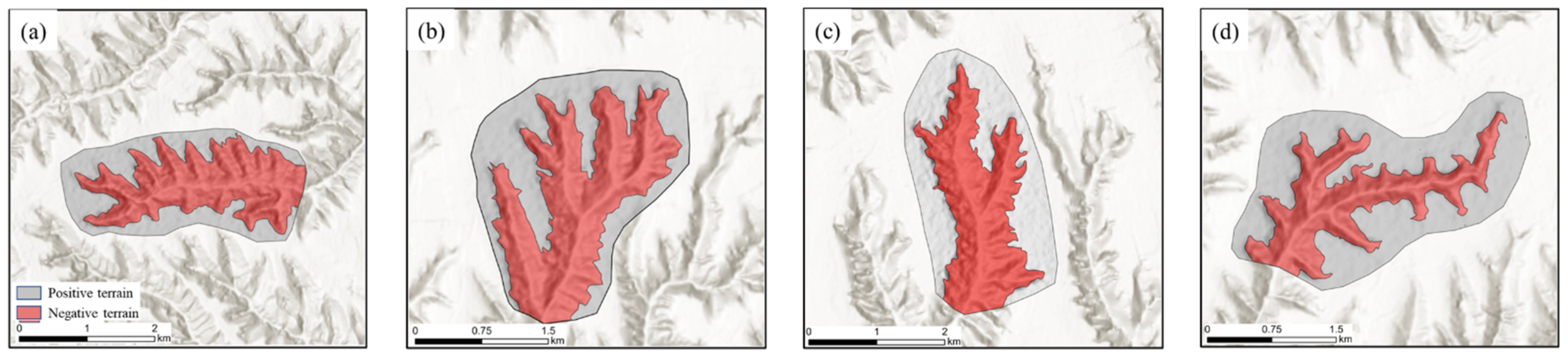
In this study, the Canny operator was used to complete the detection of the gully range on high-resolution satellite images, and the extraction results were superimposed on the image data, as shown in Figure 8. Based on the DEM data, the regional growing algorithm was used to complete the extraction of positive and negative terrain for each sample area. This study chose peaks and outlets as P-N terrain growing points, respectively. The peak and outlet points could be detected through neighborhood analysis and the watershed boundary method. In the process of growing, the same values of pixels were merged until there were no points to merge. The generated results were also superimposed on hillshade data, as shown in Figure 9. Overall, compared with high-resolution satellite images and hillshade data, the extraction results of edge detection and the regional growing algorithm were better.
To compare the performance of the regional growing and edge detection methods for the extraction of the shoulder line, the real shoulder line needed to be defined. In this paper, manual visual interpretation supported by expert knowledge was employed to extract the real shoulder line. The shoulder line extracted using the manual visual interpretation method based on high-resolution satellite images was used as the evaluation criterion. The extraction results of the regional growing and edge detection methods were evaluated by comparing the negative terrain areas of these two methods with the real shoulder line results. It can be seen from Table 2 that, for the four sample areas, the regional growing algorithm was generally better than the edge detection method when the negative terrain areas were used as the evaluation indicator. For example, sample area a, the difference between the results obtained by the regional growing algorithm and the standard results was within 12 ha, and the error was within 5%; the difference between the results obtained by the edge detection method and the standard results was within 41 ha, and the error was within 13%. These results also showed that the results of shoulder line extraction are credible when studying the characteristic indicators related to area, such as gully erosion. However, in the details, we can find that there were still differences between the two methods. The specific analysis was as follows. It can be found from Figure 10 that the regional growing algorithm was more advantageous in the detailed expression of the shoulder line, such as the turning point of the shoulder line. However, it can be found from Figure 11 that, although the edge detection method could reflect more details, the extraction results were fragmented, resulting in inaccurate positioning of the shoulder line in some places, and the generated shoulder line was discontinuous. Although DEM data do not contain more information than high-resolution satellite images, they become an advantage for the positive and negative terrain generated by the regional growing method. This is because the core of the regional growing algorithm is the determination of the growing point. We could accurately find the lowest point (the outlet) and the highest point (the peak) as the positive and negative topographic growth points based on the DEM data using the digital terrain analysis method. Furthermore, for shoulder line continuity obtained through extraction, the regional growing algorithm had more advantages.
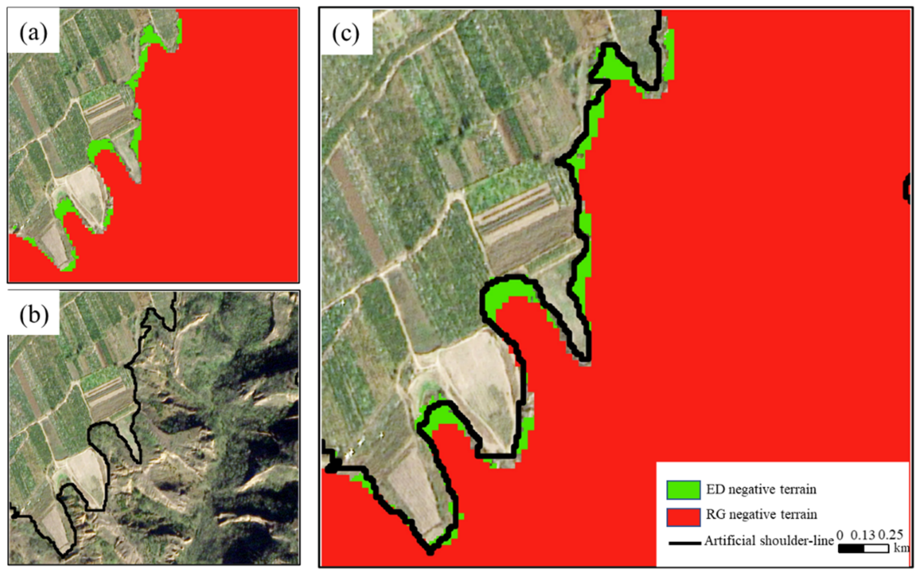
By comparing and analyzing the shoulder line obtained by manual visual interpretation of the shoulder line based on high-resolution satellite images shown in Figure 12, we can see that the shoulder line extracted by edge detection under positive and negative terrain constraints was closer to the artificial shoulder line. Therefore, the advantages of edge detection in detail and the advantages of the regional growing algorithm in continuity were combined. By using the P-N terrain constrained edge detection results obtained by the regional growing method and removing the burrs, we could finally obtain better detailed and continuous shoulder line extraction results, as shown in Figure 13.
3.3. Precision Evaluation
By comparing the CPA, PA, Dice, and IOU values, it can be seen from Table 3 that the extraction method in this study was better than edge detection and the regional growing algorithm. For example, in sample area a, the CPA value of the proposed method was 7.1% and 5.6% higher than those of the edge detection method and the regional growing algorithm, respectively. The largest PA value obtained was for the method proposed in this study, which was closer to 1, and the effect was better than those of the other methods. Similarly, both the Dice and IOU values were closer to 1, which was better than the other methods. Therefore, the reliability and accuracy of the method proposed in this study were verified.
4. Discussion
4.1. Comparison of Different Operators
For edge detection operators for different images, there are differences in edge detection. It is the premise of accurate shoulder line extraction to select an operator that is suitable for the study sample area from among many operators. Therefore, we chose sample area a to discuss the effects of common operators on the shoulder line extraction results, and the experimental results are shown in Figure 14. In this study, the line-related parameters of the shoulder line were used to further compare the detection results of each edge detection operator. These parameters were mainly used to describe the fineness of the line segment extracted by the operator. As shown in Table 4, the overall effect of the line segment extracted by the Canny operator was better than the other operators. We found that the Prewitt operator and the Sobel operator both performed differential and filtering operations on the image and only had some differences in the selection of weights for smoothing. However, the image was blurred to a certain extent, and some edges could not be detected. Therefore, the detection accuracy was relatively low, and this type of operator was deemed more suitable for situations where the gray value of an image edge is relatively obvious. The detection accuracy of the Roberts operator was relatively high, but it was easy to lose part of the edge, which made the detection results incomplete. At the same time, the image was not smoothed, and the noise could not be suppressed; thus, this operator had the best response to images with steep, low noise. The Laplace operator smoothed the image through the Gaussian function and had a relatively obvious effect on noise suppression. However, the original edge could also be smoothed during processing, resulting in some edges that could not be detected. In addition, the noise had a great influence on it; the detected image details were very rich, but at the same time, false edges could appear. If the false edges were reduced, the detection accuracy could also be reduced; many true edges could be lost, and different parameters should be selected for different images. The Canny operator was more accurate than the Laplace operator in detecting edges. Although some edge information could be lost, this operator had the best effect among the above-mentioned edge detection operators and could identify small edges more clearly.
4.2. Applications and Future Research
The landform types of the Loess Plateau in northern Shaanxi show significant regional differences, and the dominant factors of landform influence vary for different landform types. Loess landform types are mainly divided into tableland, ridges, and hills [38,39,40], and there were challenges in realizing the fully automatic extraction of the Loess Plateau shoulder line. For the Loess Plateau, it can be seen from the previous accuracy evaluation results that the proposed method had good applicability. To further verify the applicability of this method in extracting shoulder lines, we selected a loess tableland area with an area of 35,975.531 ha. The results are shown in Figure 15. By superimposing the extracted results onto high-precision images, it can be seen that the extracted shoulder lines were effective and reasonable, which verified that this method had good universality in Loess tableland area.
In loess ridge and hill regions, the terrain was more complex. As shown in Figure 16, there were many seriously discontinuous shoulder lines due to occasional gravity erosion factors, such as landslides and scattering. Some areas were also affected by artificial landforms, such as terraced fields, dams, etc., resulting in the existence of multilevel shoulder lines (Figure 16a). At the same time, in loess ridge and hill regions, due to the influence of vegetation, the slope of the shoulder line’s up- and down-slopes showed little change, and there were invisible shoulder lines (Figure 16b,c). Even if there is no interference from vegetation, in autumn and winter the continuity and visibility of shoulder lines are poor due to the impact of gravity, such as landslides, strays, and collapses, or even human factors (Figure 16d). Therefore, the application of this method in loess ridge and hill areas is also a problem that needs to be discussed and solved in the future. In future research, it is necessary to further analyze the applicability of this method for different data sources and different landform types. To better apply the method to different landform types over a large area, we could try to divide different areas according to the different land use characteristics (soil erosion characteristics and land use directions) of each landform type. On this basis, we could establish quantitative models of different shoulder lines to achieve the high-efficiency and high-precision extraction of shoulder lines.
5. Conclusions
Aiming to improve the poor continuity and inaccuracy of extracted shoulder lines, this study proposed an extraction method that fused edge detection and the regional growing algorithm. The experimental results showed that the CPA and PA values of the edge detection method were in the ranges of 77.6~83.7% and 79.1~80.1%, respectively; the CPA and PA values of the regional growing algorithm were in the ranges of 81.1~83.1% and 78.1~84.5%, respectively; the CPA and PA values of the method proposed in this study were in the ranges of 86.7~89.7% and 85.8~91.7%, respectively. Moreover, the Dice and IOU values of the method studied in this paper were closer to 1 than those of the edge detection method and the regional growing algorithm. This method could guarantee shoulder line continuity and integrity. Meanwhile, burr removal reduced errors when the grid shoulder line was transformed into a vector.
Shoulder lines have obvious turning points above and below the line, and the terrain factors (slope, curvature, etc.) also change accordingly. The geomorphic mechanisms of the P-N terrain above and below the line are significantly different. The positive terrain above the line basically maintains the original slope state after loess accumulation, and slope erosion is mainly surface erosion. The negative terrain below the line is dominated by gully erosion and gravity erosion, and various gravity landforms are widely developed. In summary, shoulder lines can be used as an important topographic index for regional soil erosion intensity and landform division. The accurate extraction of shoulder lines can provide a new perspective for the quantitative study of loess landforms and is very important for the study of Loess Plateau landforms, soil erosion characteristics, and ecological environments.
Author Contributions
Conceptualization, F.L. and H.J.; methodology, H.J.; validation, H.J., H.W. and W.L.; writing—original draft preparation, H.J., W.L. and H.W.; writing—review and editing, H.J., H.W. and W.L.; supervision, F.L.; funding acquisition, F.L. All authors have read and agreed to the published version of the manuscript.
Funding
This work was supported by the National Natural Science Foundation of China (grant number: 42271421).
Institutional Review Board Statement
Not applicable.
Informed Consent Statement
Not applicable.
Data Availability Statement
Data will be made available on reasonable request.
Conflicts of Interest
The authors declare no conflict of interest.
References
- Li, S.; Xiong, L.; Tang, G.; Strobl, J. Deep Learning-Based Approach for Landform Classification from Integrated Data Sources of Digital Elevation Model and Imagery. Geomorphology 2020, 354, 107045. [Google Scholar] [CrossRef]
- Rokosh, D.; Bush, A.B.; Rutter, N.W.; Ding, Z.; Sun, J. Hydrologic and Geologic Factors That Influenced Spatial Variations in Loess Deposition in China during the Last Interglacial–Glacial Cycle: Results from Proxy Climate and GCM Analyses. Palaeogeogr. Palaeoclimatol. Palaeoecol. 2003, 193, 249–260. [Google Scholar] [CrossRef]
- Chen, L.; Wei, W.; Fu, B.; Lü, Y. Soil and Water Conservation on the Loess Plateau in China: Review and Perspective. Prog. Phys. Geogr. 2007, 31, 389–403. [Google Scholar] [CrossRef]
- Chen, Y. Types of valleys in the loess hilly area in the middle reaches of the Yellow River. Sci. Geogr. Sin. 1984, 4, 321–327. [Google Scholar]
- Zhao, G.; Mu, X.; Wen, Z.; Wang, F.; Gao, P. Soil Erosion, Conservation, and Eco-Environment Changes in the Loess Plateau of China. Land Degrad. Dev. 2013, 24, 499–510. [Google Scholar] [CrossRef]
- Perroy, R.L.; Bookhagen, B.; Asner, G.P.; Chadwick, O.A. Comparison of Gully Erosion Estimates Using Airborne and Ground-Based LiDAR on Santa Cruz Island, California. Geomorphology 2010, 118, 288–300. [Google Scholar] [CrossRef]
- Jiang, S.; Tang, G.; Liu, K. A New Extraction Method of Loess Shoulder line Based on Marr-Hildreth Operator and Terrain Mask. PLoS ONE 2015, 10, e0123804. [Google Scholar] [CrossRef]
- Yang, X.; Li, M.; Na, J.; Liu, K. Gully Boundary Extraction Based on Multidirectional Hill-Shading from High-Resolution DEMs. Trans. GIS 2017, 21, 1204–1216. [Google Scholar] [CrossRef]
- Ke, W.; Cheng, W.; Qingfeng, Z.; Kailong, D. Loess Shoulder Line Extraction Based on Openness and Threshold Segmentation. Acta Geod. Cartogr. Sin. 2015, 44, 67–75. [Google Scholar]
- Dai, W.; Yang, X.; Na, J.; Li, J.; Brus, D.; Xiong, L.; Tang, G.; Huang, X. Effects of DEM Resolution on the Accuracy of Gully Maps in Loess Hilly Areas. Catena 2019, 177, 114–125. [Google Scholar] [CrossRef]
- Daba, S.; Rieger, W.; Strauss, P. Assessment of Gully Erosion in Eastern Ethiopia Using Photogrammetric Techniques. Catena 2003, 50, 273–291. [Google Scholar] [CrossRef]
- Castillo, C.; Pérez, R.; James, M.R.; Quinton, J.N.; Taguas, E.V.; Gómez, J.A. Comparing the Accuracy of Several Field Methods for Measuring Gully Erosion. Soil Sci. Soc. Am. J. 2012, 76, 1319–1332. [Google Scholar] [CrossRef]
- Fadul, H.M.; Salih, A.A.; Imad-eldin, A.A.; Inanaga, S. Use of Remote Sensing to Map Gully Erosion along the Atbara River, Sudan. Int. J. Appl. Earth Obs. Geoinf. 1999, 1, 175–180. [Google Scholar] [CrossRef]
- Shruthi, R.B.; Kerle, N.; Jetten, V. Object-Based Gully Feature Extraction Using High Spatial Resolution Imagery. Geomorphology 2011, 134, 260–268. [Google Scholar] [CrossRef]
- Seutloali, K.E.; Beckedahl, H.R.; Dube, T.; Sibanda, M. An Assessment of Gully Erosion along Major Armoured Roads in South-Eastern Region of South Africa: A Remote Sensing and GIS Approach. Geocarto Int. 2016, 31, 225–239. [Google Scholar] [CrossRef]
- Gafurov, A.M.; Yermolayev, O.P. Automatic Gully Detection: Neural Networks and Computer Vision. Remote Sens. 2020, 12, 1743. [Google Scholar] [CrossRef]
- Lv, G.; Xiong, L.; Chen, M.; Tang, G.; Sheng, Y.; Liu, X.; Song, Z.; Lu, Y.; Yu, Z.; Zhang, K. Chinese Progress in Geomorphometry. J. Geogr. Sci. 2017, 27, 1389–1412. [Google Scholar] [CrossRef]
- Cheng, W.; Liu, Q.; Zhao, S.; Gao, X.; Wang, N. Research and Perspectives on Geomorphology in China: Four Decades in Retrospect. J. Geogr. Sci. 2017, 27, 1283–1310. [Google Scholar] [CrossRef] [Green Version]
- Castillo, C.; Taguas, E.V.; Zarco-Tejada, P.; James, M.R.; Gómez, J.A. The Normalized Topographic Method: An Automated Procedure for Gully Mapping Using GIS. Earth Surf. Process. Landf. 2014, 39, 2002–2015. [Google Scholar] [CrossRef]
- Golosov, V.; Yermolaev, O.; Rysin, I.; Vanmaercke, M.; Medvedeva, R.; Zaytseva, M. Mapping and Spatial-Temporal Assessment of Gully Density in the Middle Volga Region, Russia. Earth Surf. Process. Landf. 2018, 43, 2818–2834. [Google Scholar] [CrossRef]
- Wei, H.; Li, S.; Li, C.; Zhao, F.; Xiong, L.; Tang, G. Quantification of Loess Landforms from Three-Dimensional Landscape Pattern Perspective by Using DEMs. ISPRS Int. J. Geo-Inf. 2021, 10, 693. [Google Scholar] [CrossRef]
- Evans, M.; Lindsay, J. High Resolution Quantification of Gully Erosion in Upland Peatlands at the Landscape Scale. Earth Surf. Process. Landf. 2010, 35, 876–886. [Google Scholar] [CrossRef]
- Lei, X.; Zhou, Y.; Li, Y.; Wang, Z. Construction and characteristic analysis of loess landform approximation factor based on DEM. J. Geo-Inf. Sci. 2020, 22, 431–441. [Google Scholar]
- Xiao, C.; Tang, G. Classification of valley shoulder line in Loess Relief. Arid. Land Geogr. 2007, 30, 646–653. [Google Scholar]
- Lv, G.; Qian, Y.; Chen, Z. Research on automatic extraction of loess landform shoulder line based on grid digital elevation model. Sci. Geogr. Sin. 1998, 18, 567–573. [Google Scholar]
- Liu, P.; Zhu, Q.; Wu, D.; Zhu, J.; Tang, X. Research on automatic extraction technology of loess area shoulder line based on grid DEM and water flow path. J. Beijing For. Univ. 2006, 28, 72–76. [Google Scholar]
- Yang, F.; Zhou, Y.; Chen, M. Shoulder line constrained loess water-erodible gully extraction. Mt. Res. 2016, 34, 504–510. [Google Scholar]
- Vrieling, A.; Rodrigues, S.C.; Bartholomeus, H.; Sterk, G. Automatic Identification of Erosion Gullies with ASTER Imagery in the Brazilian Cerrados. Int. J. Remote Sens. 2007, 28, 2723–2738. [Google Scholar] [CrossRef]
- Yan, S.; Tang, G.; Li, F.; Dong, Y. Automatic extraction of loess landform lines using DEM edge detection. Geomat. Inf. Sci. Wuhan Univ. 2011, 36, 363–366. [Google Scholar]
- Wang, K.; Wang, Z.; Zhang, Q.; Ding, K. A Loess Plateau shoulder line Extraction Method Combining Topographic Opening and Differential Image Threshold Segmentation. Acta Geod. Cartogr. Sin. 2015, 44, 67–75. [Google Scholar]
- Lira, J.; Maletti, G. A Supervised Contextual Classifier Based on a Region-Growth Algorithm. Comput. Geosci. 2002, 28, 951–959. [Google Scholar] [CrossRef]
- Ghule, A.G.; Deshmukh, P.R. Image Segmentation Available Techniques, Open Issues and Region Growing Algorithm. J. Signal Image Process. 2012, 3, 71–75. [Google Scholar]
- Liu, W.; Li, F.Y.; Xiong, L.Y.; Liu, S.L.; Wang, K. Shoulder Line Extraction in the Loess Plateau Based on Region Growing Algorithm. Int. J. Georgr. Inf. Sci. 2016, 18, 220–226. [Google Scholar]
- Basu, M. Gaussian-Based Edge-Detection Methods-a Survey. IEEE Trans. Syst. Man Cybern. Part C Appl. Rev. 2002, 32, 252–260. [Google Scholar] [CrossRef] [Green Version]
- Canny, J. A Computational Approach to Edge Detection. IEEE Trans. Pattern Anal. Mach. Intell. 1986, PAMI-8, 679–698. [Google Scholar] [CrossRef]
- Zhang, Z.; Wang, Y.; Xue, G. Digital Image Processing and Computer Vision—Visual C++ and Matlab Implementation; People’s Posts and Telecommunications Press: Beijing, China, 2010; 368p. [Google Scholar]
- Xiong, L.; Tang, G.; Yan, S.; Zhu, S.; Sun, Y. Landform-Oriented Flow-Routing Algorithm for the Dual-Structure Loess Terrain Based on Digital Elevation Models: Flow-Routing Algorithms for the Dual-Structure Loess Terrain. Hydrol. Process. 2014, 28, 1756–1766. [Google Scholar] [CrossRef]
- Xiong, L.-Y.; Tang, G.-A.; Li, F.-Y.; Yuan, B.-Y.; Lu, Z.-C. Modeling the Evolution of Loess-Covered Landforms in the Loess Plateau of China Using a DEM of Underground Bedrock Surface. Geomorphology 2014, 209, 18–26. [Google Scholar] [CrossRef]
- McVicar, T.R.; Van Niel, T.G.; Li, L.; Wen, Z.; Yang, Q.; Li, R.; Jiao, F. Parsimoniously Modelling Perennial Vegetation Suitability and Identifying Priority Areas to Support China’s Re-Vegetation Program in the Loess Plateau: Matching Model Complexity to Data Availability. For. Ecol. Manag. 2010, 259, 1277–1290. [Google Scholar] [CrossRef]
- Wei, H.; Xiong, L.; Zhao, F.; Tang, G.; Lane, S.N. Large-Scale Spatial Variability in Loess Landforms and Their Evolution, Luohe River Basin, Chinese Loess Plateau. Geomorphology 2022, 415, 108407. [Google Scholar] [CrossRef]
Figure 1.
An illustration of shoulder line of the Loess Plateau.

Figure 2.
Location of the study area: (a,b) location of Loess Plateau; (c,c1–c4) hillshade map of the study area.
Figure 2.
Location of the study area: (a,b) location of Loess Plateau; (c,c1–c4) hillshade map of the study area.

Figure 3.
Illustration of regional growth: (a–d) represent the four steps of the regional growing algorithm, respectively.
Figure 3.
Illustration of regional growth: (a–d) represent the four steps of the regional growing algorithm, respectively.

Figure 4.
Slope’s influence on the positive and negative terrain classification results: (a) represents the classification map of positive and negative terrain; (b) represents the results after slope correction.
Figure 4.
Slope’s influence on the positive and negative terrain classification results: (a) represents the classification map of positive and negative terrain; (b) represents the results after slope correction.

Figure 5.
Contrast between before (a) and after (b) burr removal.

Figure 6.
Structure elements.

Figure 7.
The complete process of our experiment.

Figure 8.
The result of extracting Negative terrain by edge detection method. (a–d) represent 4 sample areas.
Figure 8.
The result of extracting Negative terrain by edge detection method. (a–d) represent 4 sample areas.

Figure 9.
The results of extracting P-N terrain using the regional growing algorithm: (a–d) represent 4 sample areas.
Figure 9.
The results of extracting P-N terrain using the regional growing algorithm: (a–d) represent 4 sample areas.

Figure 10.
Results of edge detection compared to the regional growing algorithm: (a–d) represent 4 sample areas; (a1,b1,c1,d1) represent the results of the edge detection method; (a2,b2,c2,d2) represent the results of the regional growing algorithm.
Figure 10.
Results of edge detection compared to the regional growing algorithm: (a–d) represent 4 sample areas; (a1,b1,c1,d1) represent the results of the edge detection method; (a2,b2,c2,d2) represent the results of the regional growing algorithm.

Figure 11.
Results of the regional growing algorithm compared to edge detection: (a–d) represent 4 sample areas; (a1,b1,c1,d1) represent the results of the edge detection method; (a2,b2,c2,d2) represent the results of the regional growing algorithm.
Figure 11.
Results of the regional growing algorithm compared to edge detection: (a–d) represent 4 sample areas; (a1,b1,c1,d1) represent the results of the edge detection method; (a2,b2,c2,d2) represent the results of the regional growing algorithm.

Figure 12.
Comparison of shoulder lines between edge detection, regional growing algorithm, and manual visual interpretation. (a) represents the results of edge detection method and regional growing algorithm; (b) represents the results of manual visual interpretation; (c) represents the overlay of extraction results from different methods.

Figure 13.
Results of improved shoulder line: (a–d) represent 4 sample areas.

Figure 14.
(a) represents sample area a; (b–f) represent the extraction results of the Roberts, Prewitt, Sobel, Laplace, and Canny operators, respectively.
Figure 14.
(a) represents sample area a; (b–f) represent the extraction results of the Roberts, Prewitt, Sobel, Laplace, and Canny operators, respectively.

Figure 15.
Shoulder lines extracted by applying the method proposed in this study.

Figure 16.
Examples of landforms in loess ridge and hill regions. (a–d) show the distribution of shoulder lines in loess ridge and hill regions, respectively
Figure 16.
Examples of landforms in loess ridge and hill regions. (a–d) show the distribution of shoulder lines in loess ridge and hill regions, respectively


Table 1.
Details of data used in this study.
| Data Name | Type | Resolution | Data Resource |
|---|---|---|---|
| Satellite images | Raster | 3 m | https://www.planet.com/explorer/ (accessed on 1 September 2021) |
| DEM | Raster | 12.5 m | https://search.asf.alaska.edu/#/ (accessed on 1 October 2016) |
| Vector boundaries data | Vector | — | 1:250,000 national basic geographic database |
Table 2.
Comparison of extracted negative terrain area with standard area differences.
| Method | Indicator | Sample Area a | Sample Area b | Sample Area c | Sample Area d |
|---|---|---|---|---|---|
| Manual visual interpretation | negative terrain area (ha) | 320.912 | 328.762 | 347.209 | 197.833 |
| Regional growing algorithm | negative terrain area (ha) | 328.624 | 317.811 | 334.249 | 189.325 |
| percent error | 2.403% | 3.331% | 3.733% | 4.301% | |
| absolute error | 7.712 | 10.951 | 12.960 | 8.508 | |
| Edge detection | negative terrain area (ha) | 280.713 | 290.678 | 317.581 | 176.741 |
| percent error | 12.526% | 11.584% | 8.533% | 10.662% | |
| absolute error | 40.199 | 38.084 | 29.628 | 21.092 |
Table 3.
Comparison of accuracy evaluation index values of different algorithms.
| Sample Area | Method | CPA | PA | Dice | IOU |
|---|---|---|---|---|---|
| Edge detection | 0.814 | 0.791 | 0.818 | 0.734 | |
| a | Regional growing algorithm | 0.829 | 0.807 | 0.820 | 0.813 |
| Method in this study | 0.885 | 0.864 | 0.877 | 0.907 | |
| Edge detection | 0.837 | 0.797 | 0.820 | 0.828 | |
| b | Regional growing algorithm | 0.831 | 0.845 | 0.815 | 0.836 |
| Method in this study | 0.897 | 0.858 | 0.871 | 0.891 | |
| Edge detection | 0.776 | 0.801 | 0.843 | 0.794 | |
| c | Regional growing algorithm | 0.819 | 0.836 | 0.833 | 0.857 |
| Method in this study | 0.867 | 0.917 | 0.866 | 0.897 | |
| Edge detection | 0.801 | 0.799 | 0.791 | 0.747 | |
| d | Regional growing algorithm | 0.811 | 0.781 | 0.831 | 0.811 |
| Method in this study | 0.873 | 0.911 | 0.859 | 0.909 |
Table 4.
Comparison of evaluation index values of different edge detection operators.
| Operator Type | Number of Lines | Maximum Length (m) | Total Length (m) |
|---|---|---|---|
| Prewitt | 427 | 12,116 | 21,033 |
| Sobel | 514 | 6283 | 23,877 |
| Robert’s | 441 | 9867 | 23,196 |
| Laplace | 154 | 17,421 | 22,966 |
| Canny | 87 | 19,308 | 22,393.8 |
Publisher’s Note: MDPI stays neutral with regard to jurisdictional claims in published maps and institutional affiliations. |
© 2022 by the authors. Licensee MDPI, Basel, Switzerland. This article is an open access article distributed under the terms and conditions of the Creative Commons Attribution (CC BY) license (https://creativecommons.org/licenses/by/4.0/).
Share and Cite
MDPI and ACS Style
Jiao, H.; Li, F.; Wei, H.; Liu, W. An Improved Shoulder Line Extraction Method Fusing Edge Detection and Regional Growing Algorithm. Appl. Sci. 2022, 12, 12662. https://0-doi-org.brum.beds.ac.uk/10.3390/app122412662
AMA Style
Jiao H, Li F, Wei H, Liu W. An Improved Shoulder Line Extraction Method Fusing Edge Detection and Regional Growing Algorithm. Applied Sciences. 2022; 12(24):12662. https://0-doi-org.brum.beds.ac.uk/10.3390/app122412662
Chicago/Turabian StyleJiao, Haoyang, Fayuan Li, Hong Wei, and Wei Liu. 2022. "An Improved Shoulder Line Extraction Method Fusing Edge Detection and Regional Growing Algorithm" Applied Sciences 12, no. 24: 12662. https://0-doi-org.brum.beds.ac.uk/10.3390/app122412662
Note that from the first issue of 2016, this journal uses article numbers instead of page numbers. See further details here.