Impact of Economic Indicators on the Integrated Design of Wind Turbine Systems


Jiangsu Key Laboratory of Hi-Tech Research for Wind Turbine Design, Nanjing University of Aeronautics and Astronautics, Nanjing 210016, China
*
Author to whom correspondence should be addressed.
Appl. Sci. 2018, 8(9), 1668; https://0-doi-org.brum.beds.ac.uk/10.3390/app8091668
Submission received: 8 July 2018
/
Revised: 13 August 2018
/
Accepted: 8 September 2018
/
Published: 15 September 2018
(This article belongs to the Special Issue Wind Turbine Aerodynamics)
Abstract
:This article presents a framework to integrate and optimize the design of large-scale wind turbines. Annual energy production, load analysis, the structural design of components and the wind farm operation model are coupled to perform a system-level nonlinear optimization. As well as the commonly used design objective levelized cost of energy (LCoE), key metrics of engineering economics such as net present value (NPV), internal rate of return (IRR) and the discounted payback time (DPT) are calculated and used as design objectives, respectively. The results show that IRR and DPT have the same effect as LCoE since they all lead to minimization of the ratio of the capital expenditure to the energy production. Meanwhile, the optimization for NPV tends to maximize the margin between incomes and costs. These two types of economic metrics provide the minimal blade length and maximal blade length of an optimal blade for a target wind turbine at a given wind farm. The turbine properties with respect to the blade length and tower height are also examined. The blade obtained with economic optimization objectives has a much larger relative thickness and smaller chord distributions than that obtained for high aerodynamic performance design. Furthermore, the use of cost control objectives in optimization is crucial in improving the economic efficiency of wind turbines and sacrificing some aerodynamic performance can bring significant reductions in design loads and turbine costs.
1. Introduction
Wind turbine design is a complex task comprising multiple disciplines, requiring a trade-off between many conflicting objectives. Many research articles have been published to achieve an optimal turbine design. Some use a single objective such as maximum annual energy production (AEP) or maximum AEP per turbine weight to carry out a single-objective optimization [1]. Others use multi-objective methods [2,3] or a multi-level system design [4] to accomplish a balance between different conflicting objectives, often drawn from different scientific and economic disciplines. The objective functions of wind turbine design can be divided in four main categories: Maximization of the energy production, minimization of the blade mass, minimization of the cost of energy, and multi-objective optimization [5].
Multi-objective optimization offers a set of Pareto Optimal design solutions and places the burden of choice on the shoulders of the decision maker. In contrast, a single objective lumps all different objectives into one and provides a unique design result to the decision maker, which seems to be more practical. The difficulty is that the objective must reflect the nature of the problem. Inappropriate design goal will lead to unfeasible results. For example, maximization of the power coefficient results in larger root chords and a very high blade twist [5], while minimization of mass/AEP may overemphasize the role of the tower [6]. Hence, the selection of objective is crucial in wind turbine design.
It is noticed that the development of a wind farm is essentially an investment activity and wind turbine design is an upstream stage of wind farm development. In this case, turbine optimization also needs to be performed from an engineering economics point of view. Many economic functions such as levelized cost of energy (LCoE), net present value (NPV), internal rate of return (IRR) and discounted payback time (DPT) have been used to evaluate the profitability of wind farms [7,8]. The LCoE represents the minimum energy price that meets the desired interest rate by the designers, NPV defines the total profit of the wind farm and takes into account the price of energy, IRR is the interest rate that sets the NPV function equal to zero and enables checking if a minimum rate of return set by the designers is met, and DPT determines the time required to cover the initial investment while taking into account the time value of the money [9,10]. In these economic indicators, LCoE is the most common one used as an objective in wind turbine design [11,12,13]. But sometimes LCoE alone is not a sufficient measure to determine a project’s profitability or competitiveness. Investors need other parameters as inputs to make investment decisions [10]. However, there has been no research published using other economic indicators as objectives to perform a wind turbine design. Therefore, besides LCoE, economic functions like NPV, IRR and DPT will also be utilized as design objectives in this study. Insights into the differences between these metrics and the impact of these economic functions when used as optimization objectives will be assessed.
To carry out this research, a system-level optimization framework is used to perform an integrated design of a wind turbine. Blade length, the geometry of the blade and the tower height are selected as design variables. The purpose of this study is not to develop a design methodology, or present exact parameters for an optimized wind turbine, but rather to assess the effect of different objective functions on the properties of optimal wind turbines.
2. Methodology
2.1. Calculation Tools
Recent developments in the methodology of wind turbine design have mainly focused on simultaneous evaluation of aerodynamic and structural design [14,15,16,17]. In this paper a series of automated calculation models are coupled to perform an integrated optimization. The integrated methodology mainly builds upon that previously described in References [6,16], which includes the rotor aerodynamic analysis, blade structure design and cost model. These models are selected as a compromise between computational effort and calculation accuracy. The integrated design strategy has been successfully used in the design of a 1.5 MW stall regulated rotor [14], BONUS 1 MW and WM 600 wind turbine [18], and the investigation of 5 MW upwind and downwind turbines [16], proved to be effective in the wind turbine optimization.
In the next subsection we describe how the integrated modelling tool is implemented, giving details of how the models are coupled and how the optimization process is sequenced.
2.1.1. Power Production
Aerodynamic analysis is based on ordinary blade element/momentum (BEM) theory. A detailed description of the process with an extensive explanation of its fundamental equations can be found in Reference [19]. AEP is computed using a Rayleigh distribution in which mean speed varies with the hub height. An exponential law is used to calculate the average wind speed at different hub heights as follows:
where is the reference height, is the average wind speed at and is the wind shear exponent.
2.1.2. Loading
Load calculation is an important discipline within wind turbine technology. Design loads serve as inputs for the structural design of rotor blades and other turbine components, and essentially determine the cost of producing a wind turbine. Typically, load analysis is performed using dynamic simulation software such as “DNV Bladed” according to the IEC61400-1 standard [20] during the real-world wind turbine design process. However, this load estimation procedure is difficult to carry out in the optimization period for the following reasons:
- For an accurate estimation of design loads, there are thousands of design load cases (DLCs) which must be simulated, causing a significant computational cost. Design optimization of a wind turbine requires estimations of hundreds of thousands of different turbine configurations. For this reason, a full IEC loads analysis is not computationally feasible.
- The output loads are influenced by the controller algorithm. For example, coefficients in the PID controller and pitch rates under different operational conditions can have a significant effect. Typically, we must modify many parameters of the controller to find the best controller algorithm and configuration for a given wind turbine. This is another computationally expensive aspect which limits the usefulness of automated design load analysis.
Some approaches have been described to deal with this problem. For example, some essential load cases can be selected to reduce the computational cost [18]. It is also possible to use the static forces of rotor and tower at some critical conditions, with an amplification factor to correct for dynamic effects [16]. In accordance with the latter approach, we explored a series of load calculation results from commercial wind turbines, correlated the conditions a wind turbine experiences when ultimate loads occur (rotor speed, wind speed, pitch angle, azimuth angle, etc.), and then identified the appropriate static load cases (SLCs) to perform the loads estimation, which are summarized in Table 1.
SLC 1.1 represents an extremely gusty wind condition. The ultimate loads on a wind turbine are more likely to happen in gusty conditions near the rated wind speed, typically due to a rapid increase of wind speed which the pitch angle can’t catch up with. SLC 1.2 examines the operational condition IEC DLC 1.3, with an extreme turbulence model. In this case the maximum wind speed will increase to a very high value in a short period due to extreme turbulence at the cut-out wind speed. SLC 2.1 and 2.2 represent the parked survival cases of wind turbines under extreme conditions which occur every 1 year and every 50 years, respectively.
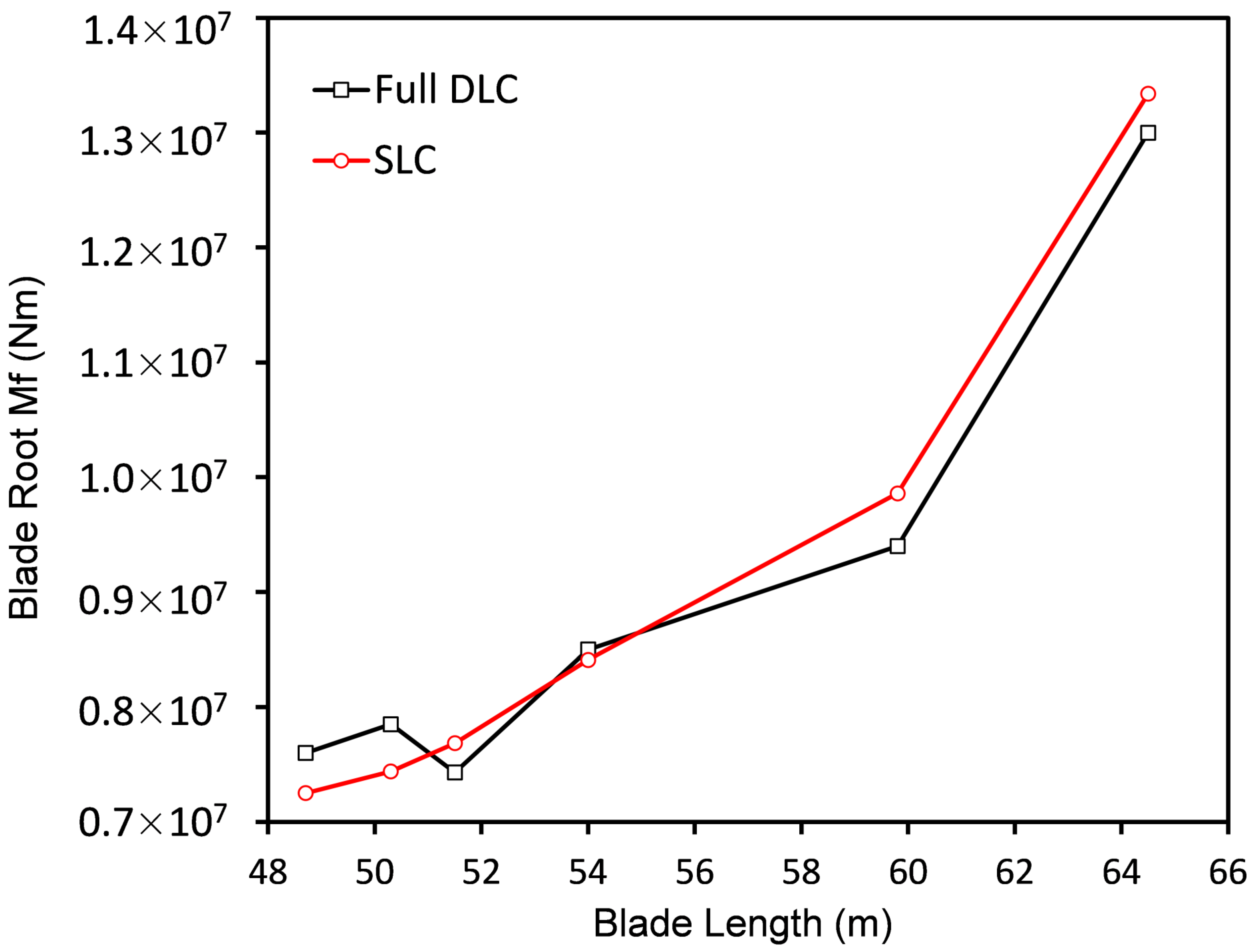
The predicted static thrust from the blade requires a dynamic amplification factor of 1.45 to fall within the range of dynamic loadings from “DNV Bladed” simulations. To check the feasibility of this assumption, we carried out several load estimations for different wind turbines with various blade lengths. Figure 1 shows the comparison of blade root flap-wise moments (Mf) between the SLCs and a more rigorous DLCs calculation procedure.
Although there is some deviation between the calculated loads, the errors are within an acceptable range. Usually the output loads on a turbine blade will increase with the blade length, however, the load evaluation of real-world turbines shows that sometimes longer blades can have lower output loads. This is mostly due to variations in the turbine configuration and control algorithms. If this influence is eliminated, we can expect that the error between the load trends in the DLC and SLC calculations would be reduced. Moreover, since the load calculations as well as the cost model described in the next section inevitably need to be simplified, the primary goal of this study is not to present an exact geometry for an optimized wind turbine, but to assess the effect of different objective functions on the properties of optimal wind turbines. For this purpose, the SLC method is more suitable.
2.1.3. Cost Model
Besides AEP, capital expenditure (CAPEX), operational expenditures (OPEX) and financing are needed as inputs to perform overall economic analysis. These are calculated using the models described in this section.
The CAPEX herein represents the overall cost of a single wind turbine. It includes turbine manufacturing cost and the sharing portion of wind farm construction and maintenance costs. The manufacturing cost uses the individual component masses for the turbine to evaluate the costs of individual components. The blade mass is derived by a structural model using beam finite element theory and classical laminate theory to determine the effect of the design loads [2]. The blade structure is formed from a double web I-beam. The material used for the bulk of the blade is glass fiber with reinforced polyester and foam.
A set of physics-based models are used to estimate the sizes and costs of a subset of the major load-bearing components (the main shaft, gear box, bedplate, gearbox, tower) and parametric formulations representative of current wind turbine technology are used to evaluate sizes and costs for the remaining components (the hub and yaw system). For example, the hub is treated as a thin-walled, ductile, cast iron cylinder with holes for blade root openings and main shaft flanges. The bedplate module is separated into two distinct front and rear components. The rear frame is modelled as two parallel steel I-beams and the front frame is modelled as two parallel ductile cast iron I-beams. The physics-based models have internal iteration schemes based on system constraints and design criteria, which are described in Reference [21].
The balance-of-station costs vary with the rotor diameter and tower height, and the OPEX are accounted for by taking a small, fixed percentage of the capital cost as the annual maintenance cost [18]. Decommissioning costs are also considered in this model.
2.2. Objective Function
The appropriate choice of an objective function is critical to an optimization process. In order to perform the wind turbine optimization from an economic point of view and ensure the designs correctly assess fundamental trade-offs (primarily between energy capture and overall cost) we chose LCoE, NPV, IRR and DPT as design metrics. The models employed in this research are proposed in Reference [10] and shown in Table 2. Dynamic evaluation of these economic functions can also be found in References [22,23].
In the economic models, the total utilized energy output and the total cost over the lifetime of the wind turbine are both discounted to the start of operation.
2.3. Design Variables and Constraints
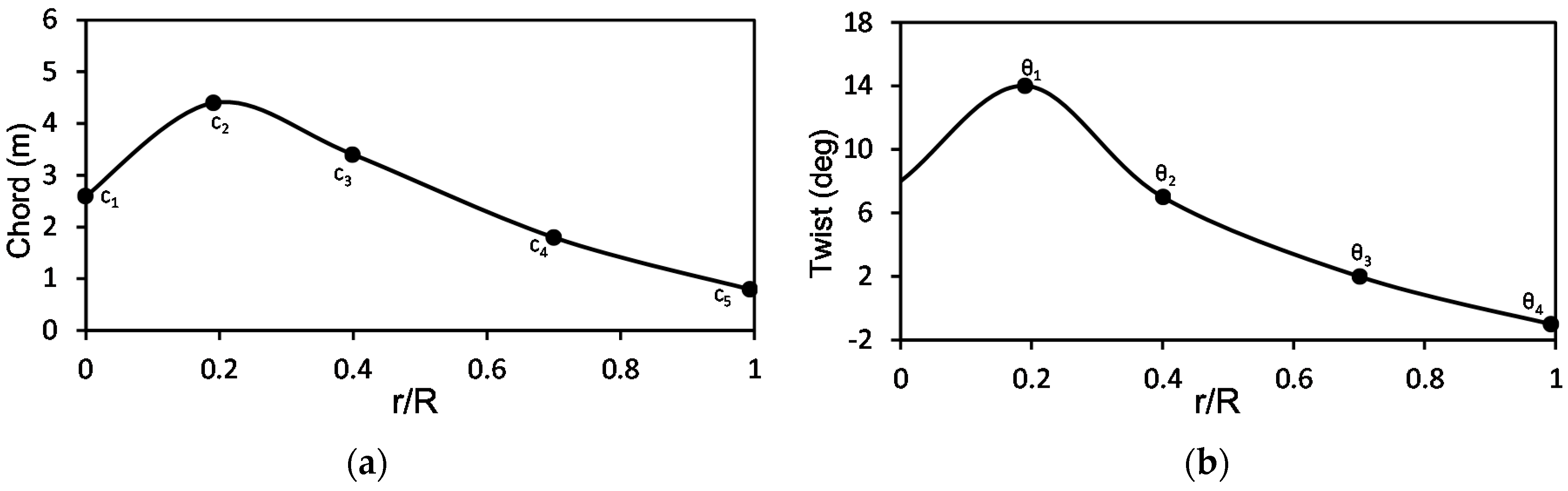
There are a total of 15 design variables used in the optimization process. B-Spline curves are used to create smooth distributions of chord, twist and relative thickness of the blade. Five control points are used to shape the chord distribution and a further four points are used to describe both twist and relative thickness distribution, as shown in Figure 2.
Blade length and tower height are also set as variables for the purpose of determining the most suitable rotor diameter and tower height for a specific wind speed site. Upper and lower limits for these variables are implemented to define the bounds of the design space.
The DU and NACA 64 series airfoils are employed in this study, as shown in Table 3. These airfoils are optimized for high speed wind condition with an advantage of high maximum lift coefficient and very low drag over a small range of operation condition. They have been used by various wind turbine manufacturers worldwide in over 10 different rotor blades for turbines with rotor diameters ranging from 29 m to over 100 m [24].
Blade structure design is set to meet the needs of strength and deflection constraints. The maximum velocity of the blade tip is 80 m/s. The rated rotational speed and the gearbox ratio change with the blade length in proportion to keep the generator operational speed the same. To have a safe blade-tower-clearance, a constraint for the blade out-of-plane deflection is used and the clearance between the ground and the blade tip is constrained by a minimum of 25 m [25].
To examine wind turbine designs at low speed sites, the average wind speed is set as 6 m/s at a reference height of 70 m. The wind shear exponent is set to be 0.2 for normal wind profile model according to the IEC61400-1 standard [20]. The power transfer efficiency is 92% and losses such as those caused by wake interference, electrical grid unavailability and air density correction are estimated using an array loss factor and an availability factor. An overall correction factor of 0.64 is used in this research.
2.4. Genetic Algorithm
The genetic algorithm (GA) is a search procedure based on genetics and natural selection mechanisms, which has proved to be efficient and robust for wind turbine system [26], wind turbine layout in wind farms [27], and offshore wind turbine support structures [28].
In this study, multi island genetic algorithm (MIGA) is employed for the optimization. In MIGA, the population is divided into several subpopulations staying on isolated “islands,” whereas traditional genetic algorithm operations are performed on each subpopulation separately. A certain number of individuals between the islands migrate after a certain number of generations. Thus, MIGA can prevent the problem of “premature” by maintaining the diversity of the population [29]. Table 4 presents the main parameters of MIGA.
3. Description of the Optimization Process
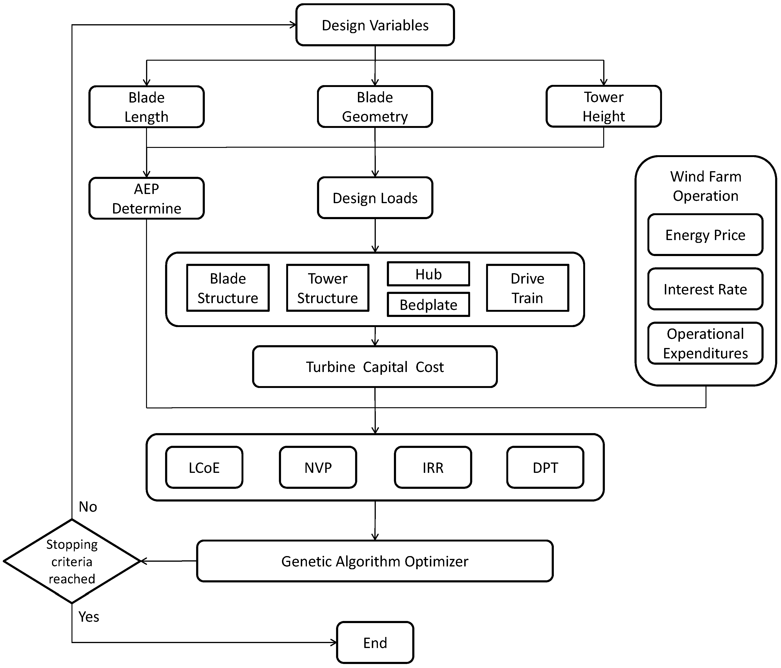
All sequential programming methods and the optimization processes are formulated in a framework. Figure 3 shows the full optimization methodology adopted in this study. Parameterization, geometry generation, AEP and load evaluation, structural design, mass and cost estimation, and economic analysis are presented in the flow chart.
Objectives such as LCoE and NPV are specified at the beginning of the optimization process. The AEP and design loads are evaluated by BEM theory, followed by calculation of the component masses and costs with the consideration of the design loads. The turbine capital cost and AEP together with the wind farm operational model are used to obtain the economic characteristic during the whole wind turbine life cycle as the final design target. The variables are changed in the optimization depending on the design objective. The maximum number of iterations is the stopping criterion. When stopping criterion is reached, the design result is picked out by the algorithm.
4. Results and Discussion
4.1. 2 MW Case Study
Recently, increasing numbers of low wind speed sites have been developed, and the 2 MW turbine is dominating the market (In 2017, the average rated power of the new installed wind turbine in China is 2.1 MW [30] and China alone accounted for 37% of the world’s new installed capacity [31]). Thus, this paper will focus on the optimization of 2 MW low wind speed turbines to capture the industrial trends of the state-of-the-art wind farm.
As the market energy price, labor costs, material costs, etc. vary between countries, the parameters considered for this case study are mainly derived from the industry’s status in China. For example, the NPV is calculated with a market energy price of 8.8 cents/kWh, the weight unit price of the blade is set to be $5.88/kg and $1.54/kg for the tower. A discount rate of 8% and an economic lifetime of 20 years are employed in this study.
The results of the optimization are presented in the following sections. Optimization outputs using different design targets are examined. Fundamental differences and observations from each case are discussed below.
4.2. Effects of Blade Length
Increasing blade length will increase energy production, but it will also increase the costs of material, labor and delivery. Generally, the initial capital cost and maintenance cost will also increase. To analyze how blade length impacts the economic effectiveness of a design, we recorded the trends in energy production, loading, mass, and costs from the properties of all the intermediate cases during the optimization. These data points are results for all metrics put together, show clearly the relationships between various turbine properties and the blade length.
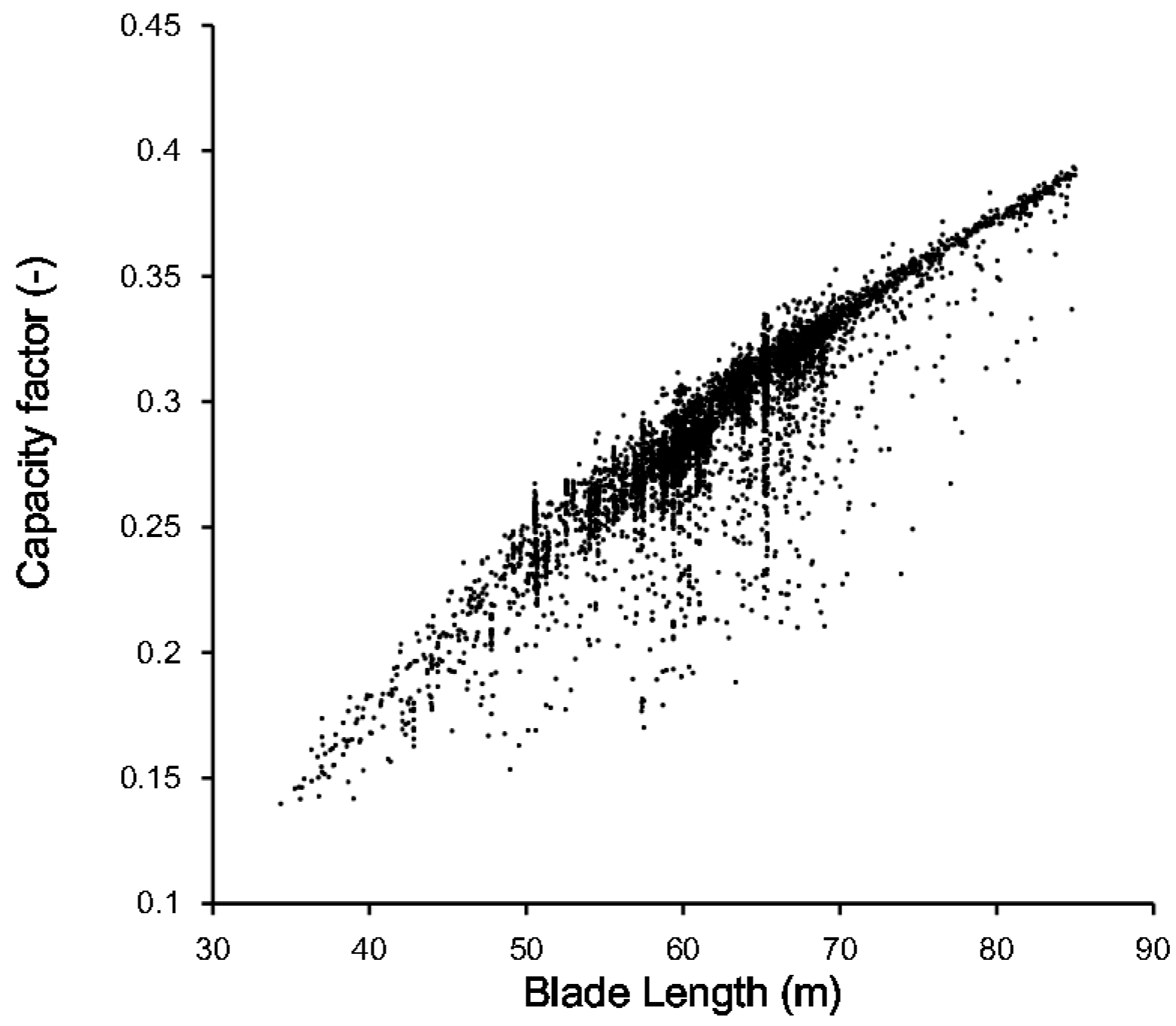
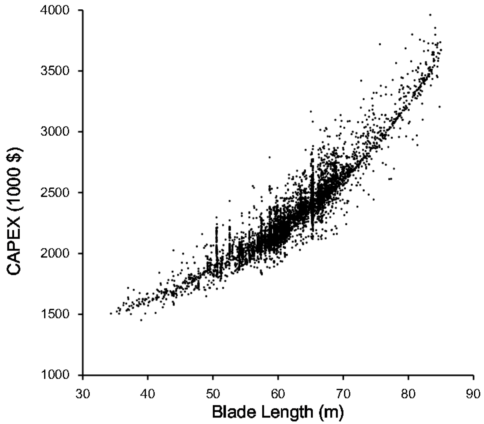
The annual capacity factor is commonly used as an indicator of energy performance. It is defined as the energy generated during the year divided by wind turbine rated power multiplied by the number of hours in the year. Figure 4 shows the capacity factor against blade length. Each point in the scatter plot represents an individual turbine configuration evaluated during the genetic algorithm. Although wind energy is proportional to the square of blade length, due to the limitation of generator capacity, the output electrical power is not permitted to exceed the rated power beyond the rated wind speed. The total energy production increases with the blade length while the effect is reduced as the blade length increases. The capital expenditure also increases with blade length, however in this case the effect increases as blade length increases (Figure 5).
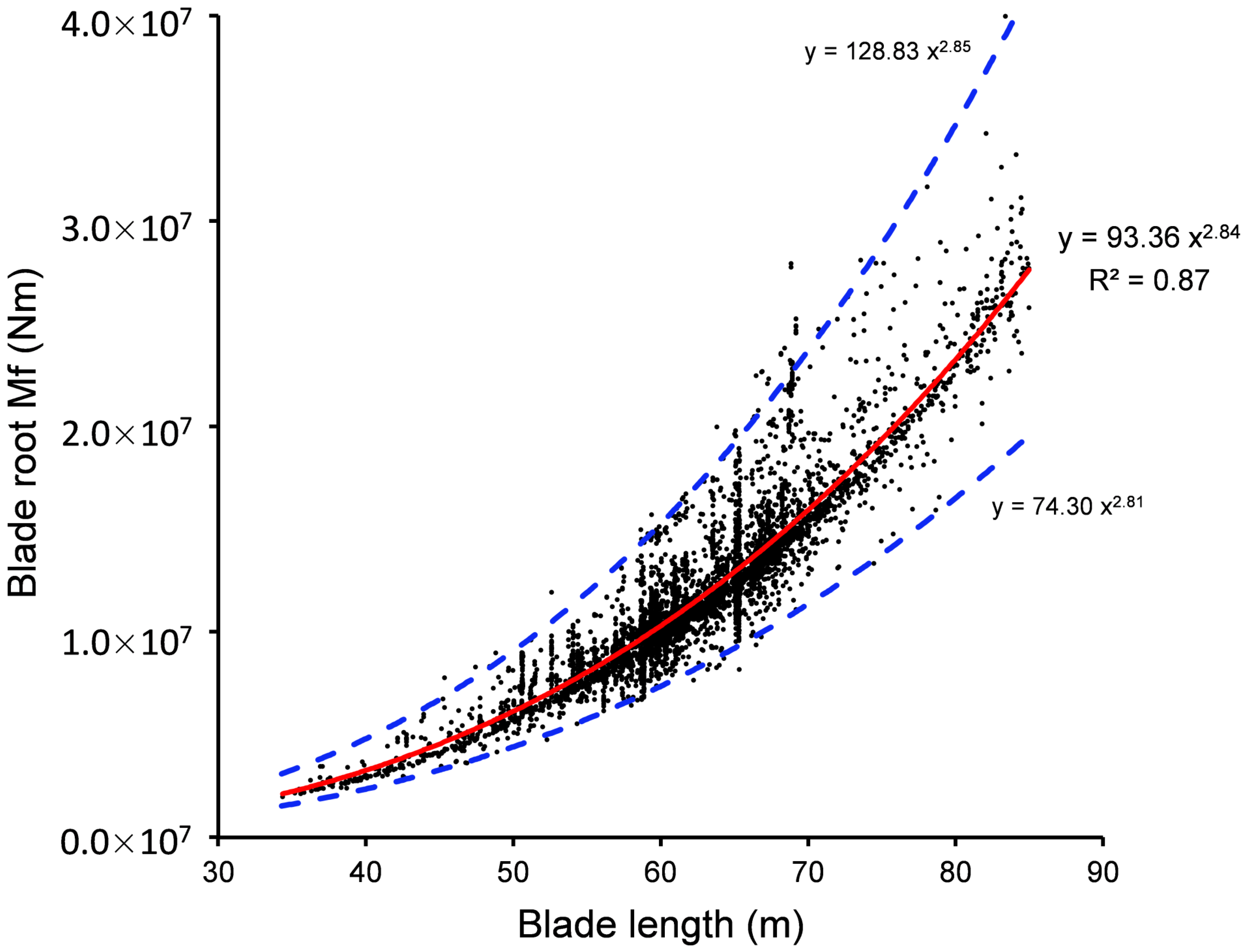
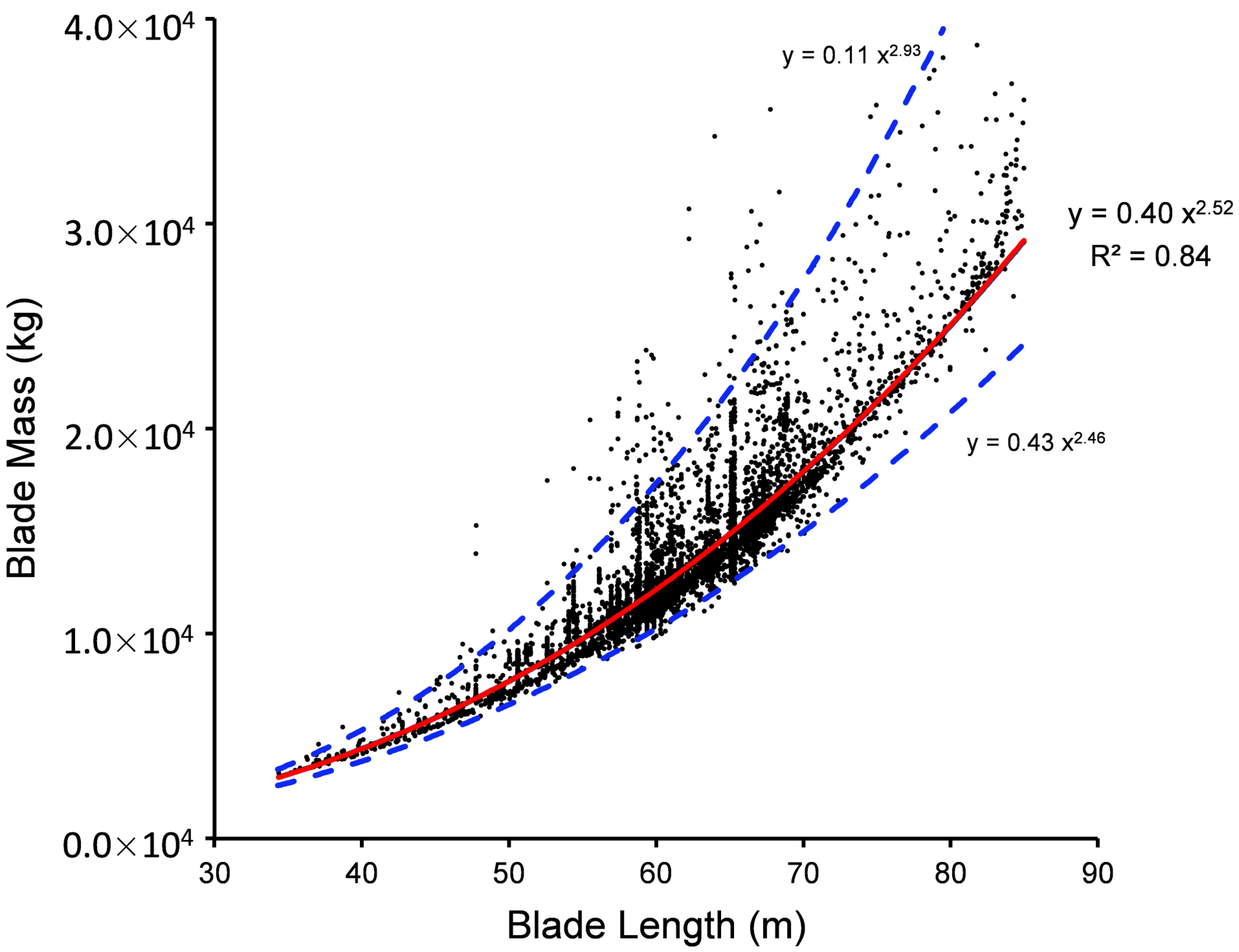
The same comparison was made for blade length against blade root loading and against blade mass, as shown in Figure 6 and Figure 7 respectively. Power law relationships are fitted to this data to quantify the correlations. The flap-wise bending moment (Mf) is the critical load in blade structure design. This research shows that the flap-wise bending moment of blade root increases with length, L, as L2.84, while the mass of the blades scales with L2.52. The enveloping functions on the outer border of the scattered points are also presented to indicate the boundary of the design results.
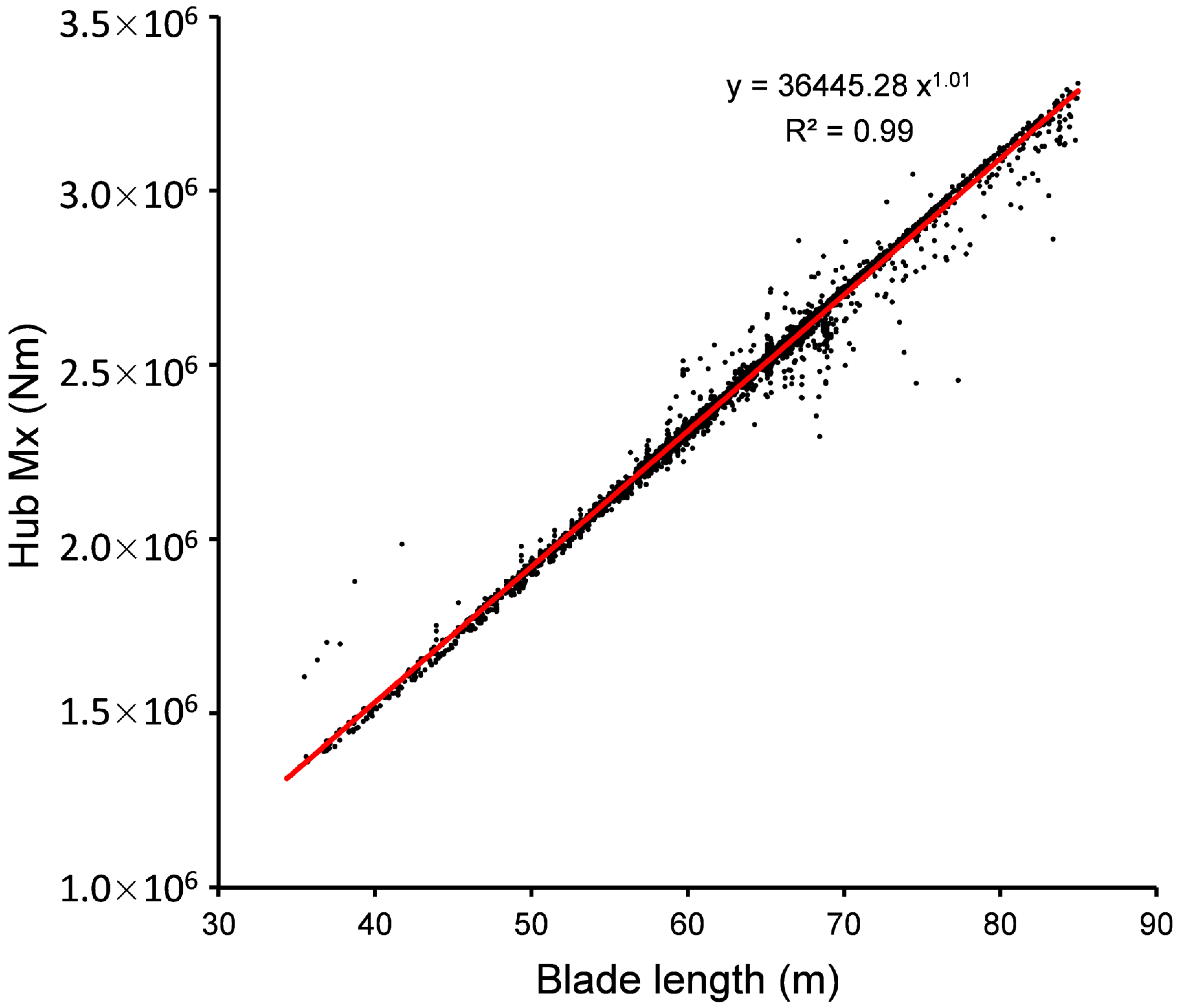
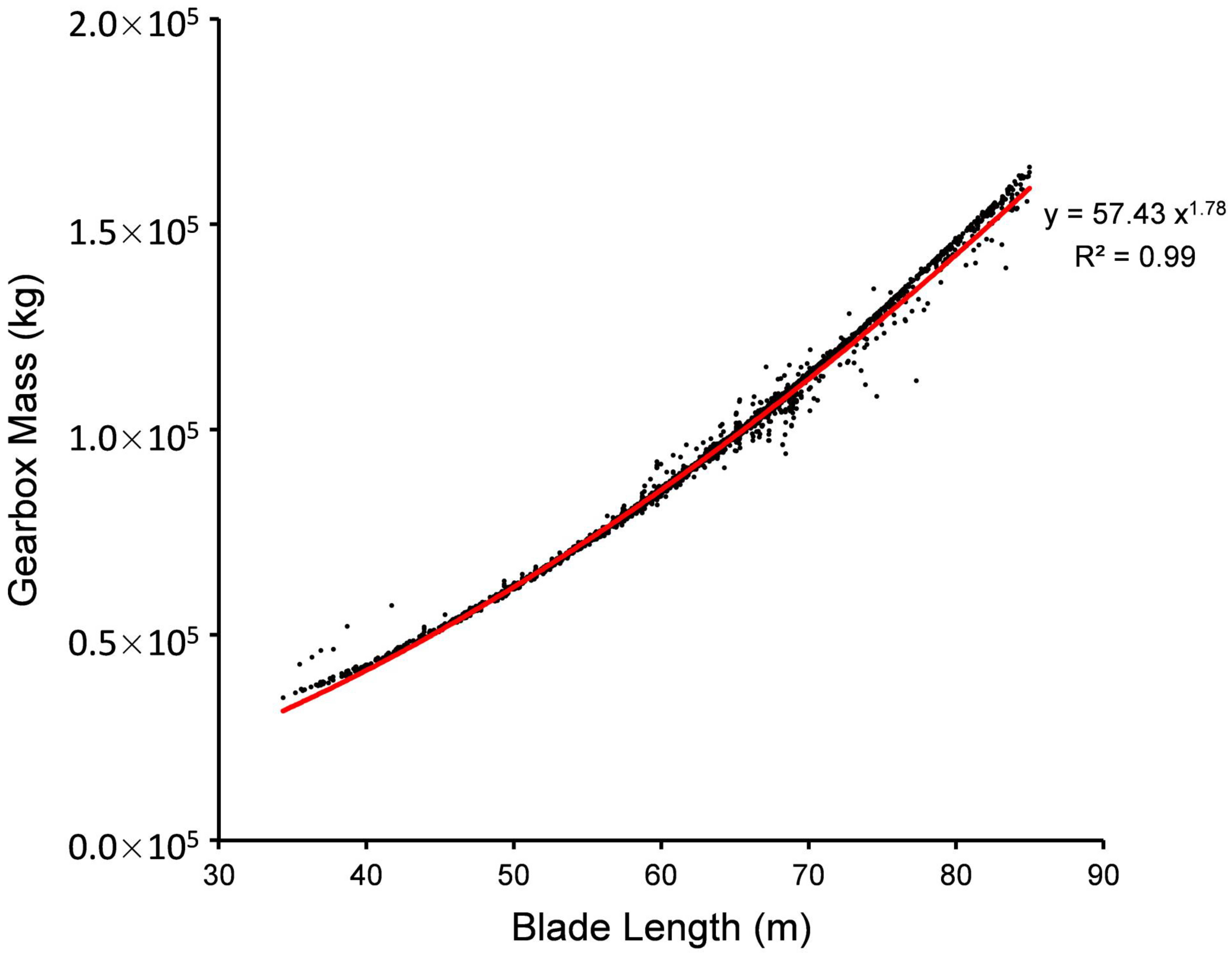
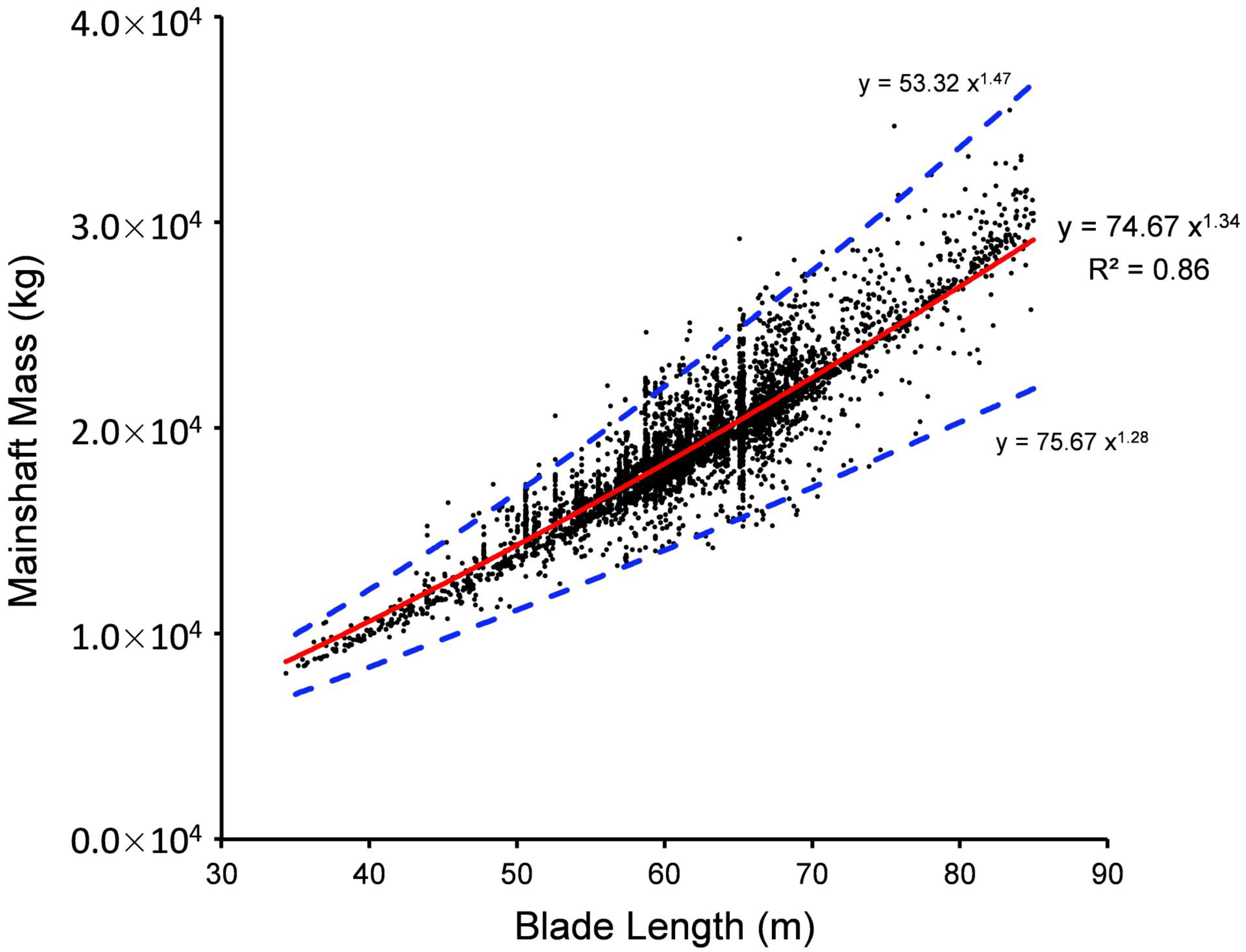
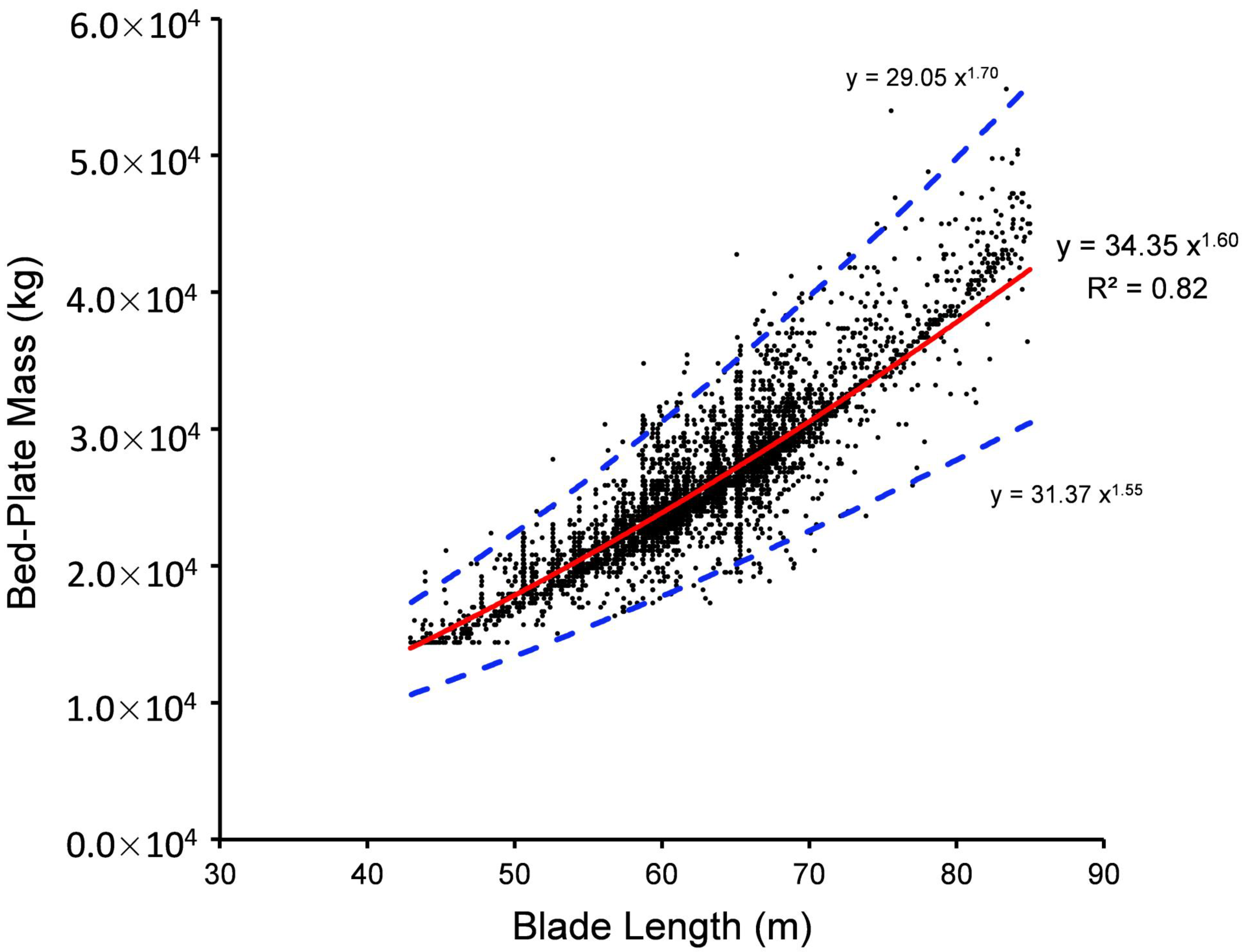
Torsional moment (Mx) under fixed hub coordinates greatly influences the gearbox design so this is examined closely in this work. The optimization data trend predicts that Mx increases linearly with L as depicted in Figure 8. Meanwhile, Figure 9 shows the gearbox mass scales as L1.78. The loading and mass of the remaining components such as the low speed shaft (Figure 10) and the bed-plate (Figure 11) each have different scale exponents as described in the figures.
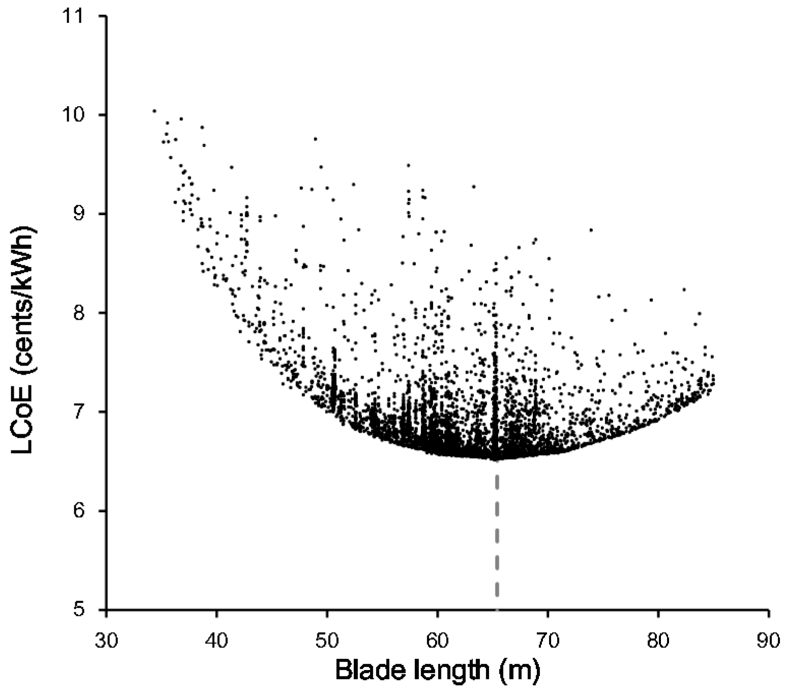
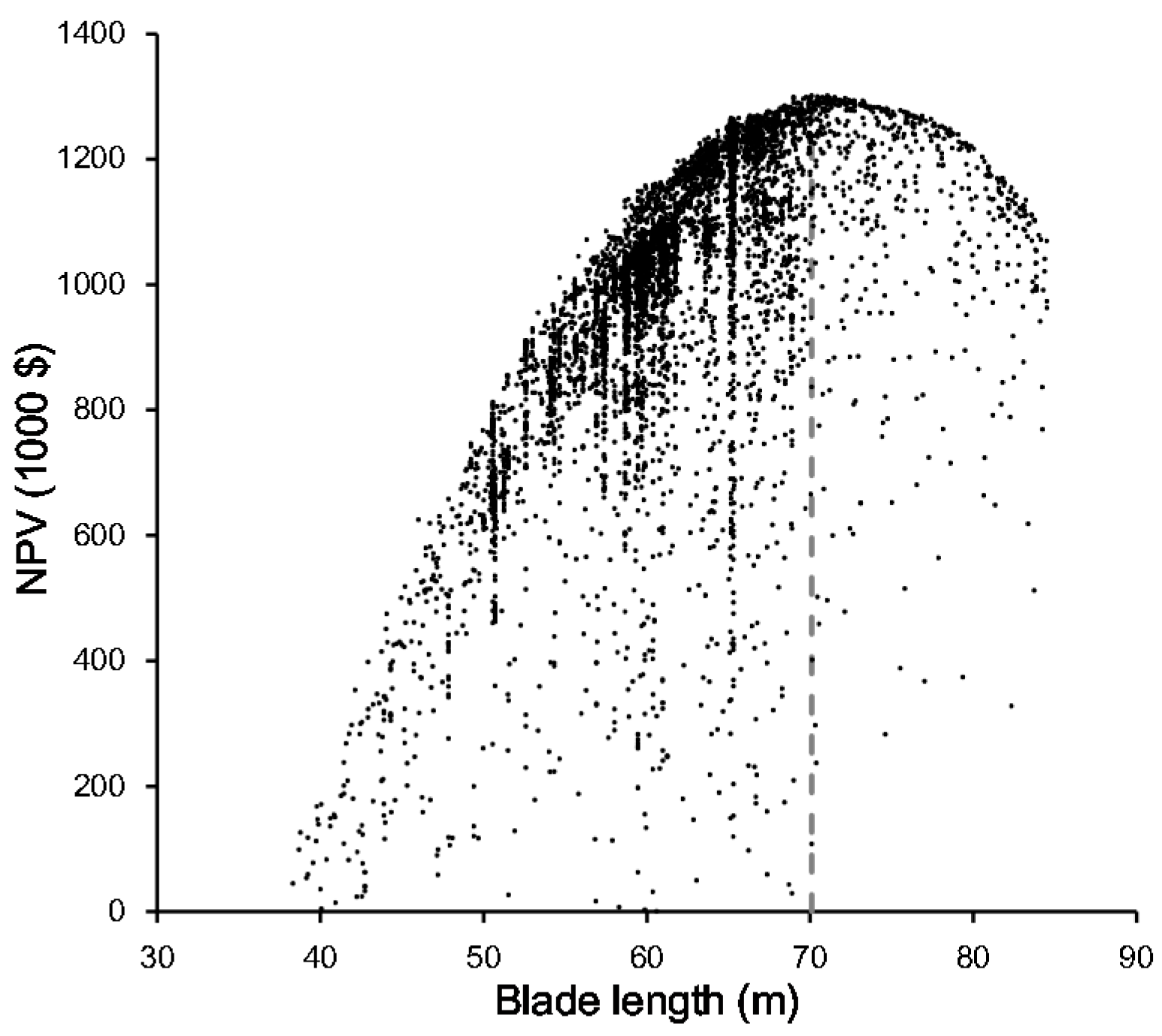
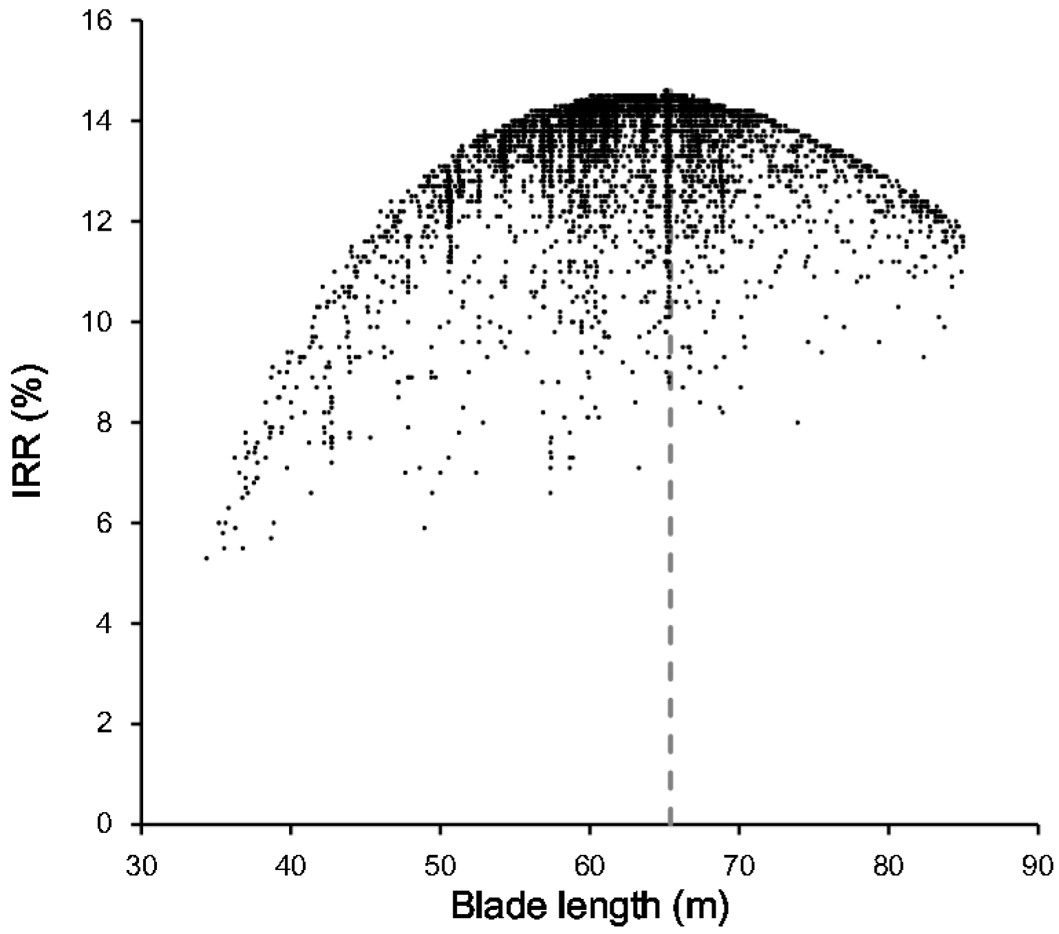
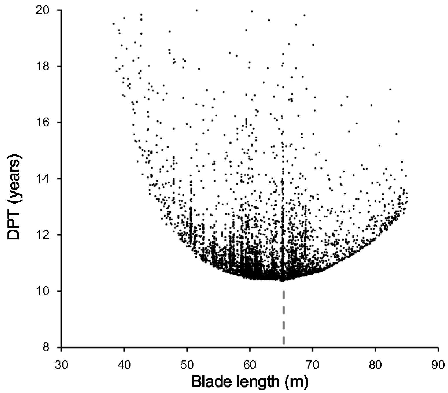
In the scatter plots of economic indicators as a function of blade length, the boundaries of these scatter cloud appear in the form of a parabola. The data points to an optimal blade length for each of these economic metrics are shown in Figure 12, Figure 13, Figure 14 and Figure 15.
A large proportion of the initial capital costs are unrelated to the rotor diameter or design loads, for example the generator, converter and control system costs. This leads to a higher LCoE and lower NPV when blade length is comparatively short. For example, a 30 m–38 m blade is uneconomical for a 2 MW turbine since the energy production is inadequate compared with the costs (Figure 13). As the blade length increases beyond 38 m, the benefits outweigh the economic costs. The economic efficiency improves until it reaches a maximum at a certain blade length. Beyond this length, the turbine may produce more energy, but due to higher manufacturing effort and increased loading on many components, the increase in cost exceeds the improvement in AEP, resulting in a lower economic efficiency.
As a result, LCoE first decreases then increases with blade length. The characteristic of NPV is just the opposite. Optimal blade length and corresponding values for LCoE and NPV can be observed. LCoE achieves a minimal value of 6.54 cents/kWh at a blade length of 65.4 m, while the NPV reaches a maximum value of $1,295,000 when the blade is 70.1 m long. The same configuration that had the lowest LCoE also presented the best values for the IRR and DPT. The highest IRR is 14.6% and the shortest DPT is 10.4 years.
4.3. Economic Functions
Based on the equations presented in Table 3, as previously assumed, OPEX are accounted for by taking a fixed percentage of the capital cost (), after some mathematical transformation, it can be found that the task of minimization of LCoE, maximization of IRR and minimization of DPT can be considered as a task to minimize the ratio between CAPEX and the AEP:
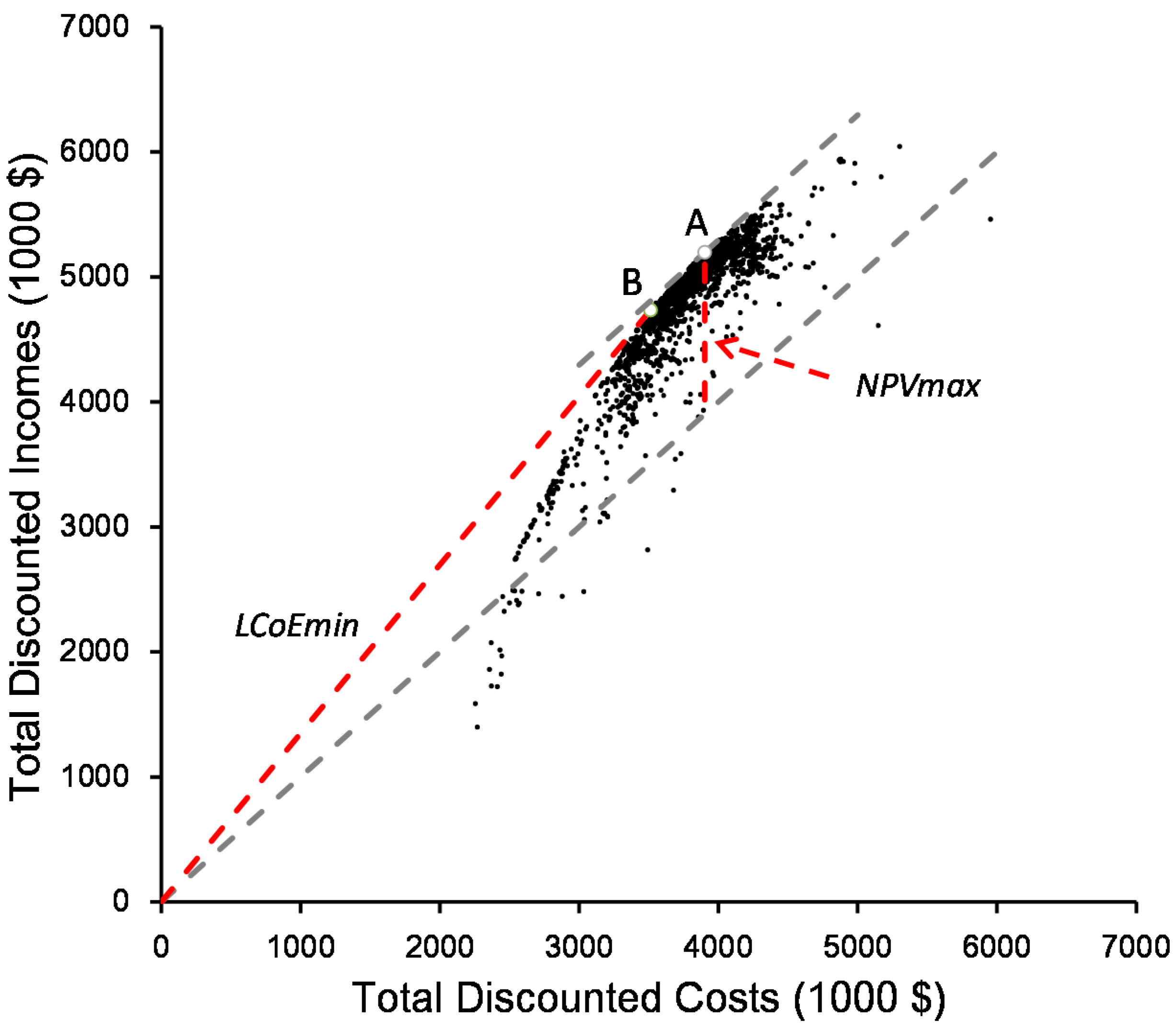
Consequently, optimum LCoE, IRR and DPT occur at the same turbine configuration while optimum NPV is achieved at an entirely different design point. Maximum NPV is achieved when the margins between total discounted income and total discounted costs are maximized. As seen in Figure 12 and Figure 13, the optimum NPV occurs at a larger blade length than the optimum LCoE.
Figure 16 illustrates the variation of total discounted incomes of different wind turbines as a function of their total discounted costs. The dashed line in the middle is the break-even line, while turbines above the line are economic and those below the line are not. Two points have been highlighted on the cost-income front. Point A, with total discounted costs of $3.9 m, has the highest net profit margin between incomes and costs which implies the maximum NPV is achieved. The investment returns of designs with costs higher than point A decline. Point B, with total discounted costs of $3.5 m has the maximum slope which indicates that the ratio between incomes and costs is maximized. This point corresponds to minimum LCoE. In this optimization problem, a wind turbine designed with the objective of minimum LCoE tends to choose a smaller-scale investment compared with the objective of maximum NPV.
The choice between LCoE and NPV is a complex economic problem. Investment size and incremental internal rate of return may also be taken into consideration to make the decision that most meets the desire of the designers. Further exploration is beyond the scope of this research. Nonetheless, the result obtained herein, that the optimal blade length of a certain turbine should be situated between the value of optimal LCoE and optimal NPV, may be valuable to wind turbine manufacturers.
4.4. Discussion of the Optimization Blades
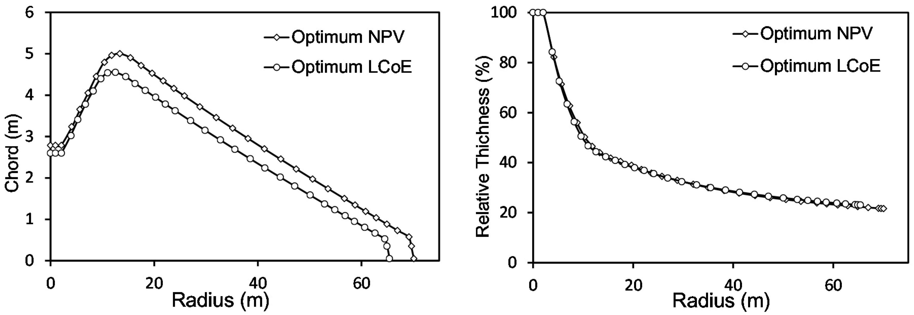
In addition to the different blade lengths obtained from these metrics, the detailed turbine configurations show the effect of several other variables. In the following subsection, optimization results are presented to provide insight about the impact of blade geometry to the integrated turbine performance. Blade shapes of optimum NPV and optimum LCoE are plotted in Figure 17, and the turbine properties with respect to these blades are summarized in Table 5.
The design providing an optimal NPV has a larger chord distribution along the full blade span, but the difference remains almost constant up to the blade tips, revealing a certain degree of similarity between these two blades. Both blades have a relatively high thickness-to-chord ratio along the blade span. The minimum relative thickness is 21.6% for optimal NPV and 23% for optimal LCoE. Though large relative thickness will undoubtedly reduce blade aerodynamic performance, the beneficial aspect is that larger section thickness can increase the section moment of inertia, which is helpful in increasing both strength and stiffness, consequently reduces the blade mass. This configuration is mainly the result of a trade-off between aerodynamic performance and blade structure. Additionally, the reduced lift characteristic of high relative thickness airfoils may also be helpful in controlling the aerodynamic loads.
Generally, neither optimum LCoE design nor optimum NPV designs tend to pursue a maximum electricity production. The maximum power coefficients (Cp) of both blades are about 0.46, which is a relatively low value by current industrial standards. Note that the optimization procedure can achieve a Cp of 0.487, as shown by the High Cp design in Table 5. One of the main reasons for this is that the increase of Cp is always associated with an increase in design loads and consequently the initial capital cost.
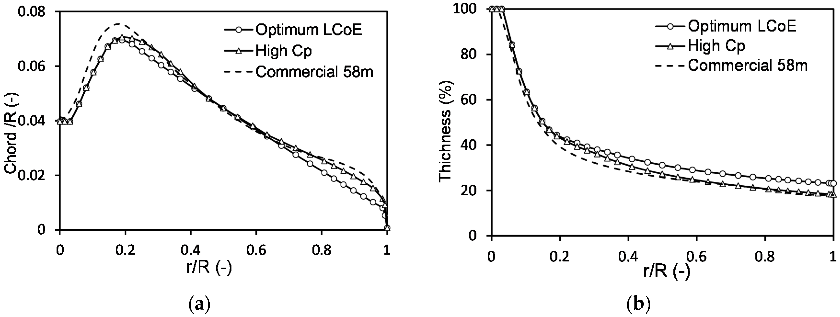
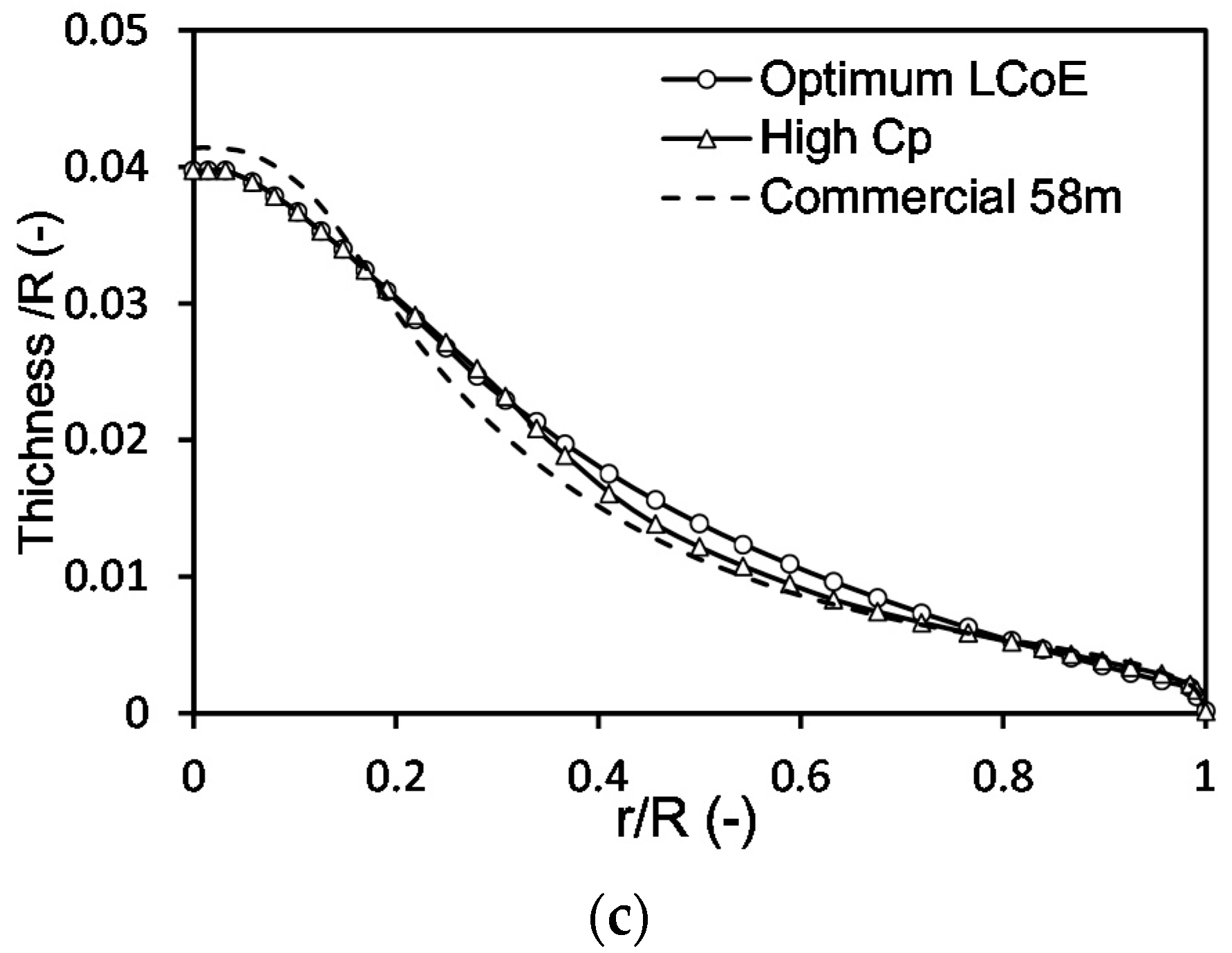
In order to elucidate why optimization designs based on economic analysis lead to relatively lower AEP, we chose the High Cp design from Table 5, which shares the same blade length and tower height as optimum LCoE. A commercial 58 m blade with a maximum Cp of 0.49 is also presented for comparison, as is shown in Figure 18. This commercial blade holds a geometry layout more similar to High Cp design, shows that some industrial practices are using the design strategy of maximum aerodynamic performance.
The turbine performance of High Cp design differs greatly from the optimum LCoE design as presented in Table 5. Generally, the design loads and the mass of structural components rise considerably.
The minimum LCoE design has a much larger relative thickness distribution along most of the blade but a smaller chord distribution at the blade tip compared with the High Cp design. This is because the minimum LCoE sacrifices rotor performance to reduce thrust and decrease turbine costs. As a result, the design loads are significantly reduced. For example, the flap-wise moment of the blade root is reduced by 9%. Together with a larger blade thickness at the mid span, which is beneficial to the structural integrity of the blade, the blade mass is reduced from 17.3 tonnes to 14.5 tonnes, a decrease of 16%. The expense is that the maximum power coefficient is reduced from 0.487 to 0.457.
0.457 may seem as unacceptable compared with 0.487, a decrease of 6.2%. However, the AEP is only degraded by 3%. Meanwhile, the design loads and structure masses were reduced significantly, accounting for a reduction in capital expenditure by 9.3%. The result produces 4.1% less LCoE and the NPV is increased. The LCoE design could be a more reasonable choice from the economic point of view.
4.5. Optimization of the Tower Height
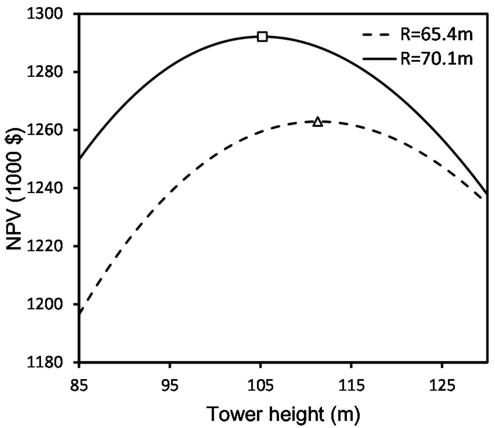
At a certain wind shear exponent, the quality of the wind improves with increasing tower height. However, the higher tower results in a heavier structure which increases the cost. Therefore, the tower height of the turbine should match the site and rotor to achieve maximum economic efficiency [32,33]. An analysis was conducted to examine the impact of the tower height on the LCoE and NPV. Both are depicted graphically in Figure 19 and Figure 20.
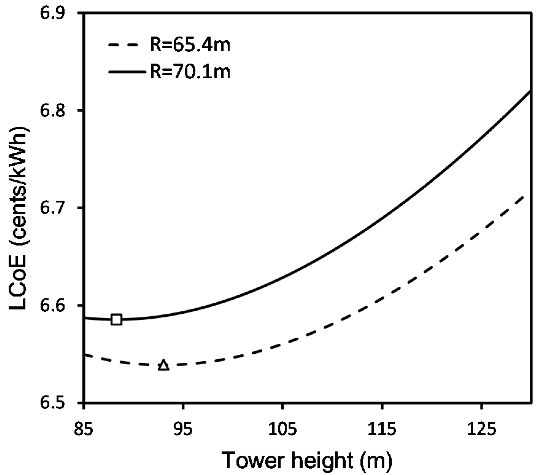
We took the rotors obtained from the optimization for examination. One is equipped with a 65.4 m blade and the other with 70.1 m blade. There are local optimum values of LCoE and NPV as a function of the tower height. The reason for this is similar to that which describes the influence of the blade length. The economic efficiency increases first and then decreases with the tower height, due to an increase in the costs of rotor, tower and the balance-of-station. Although the increased tower height can produce more energy, the increase in cost eventually outweighs the increase in profits. The optimum NPV design results in a higher tower than the optimum LCoE design, showing again that a minimum LCoE design is more geared towards controlling the cost.
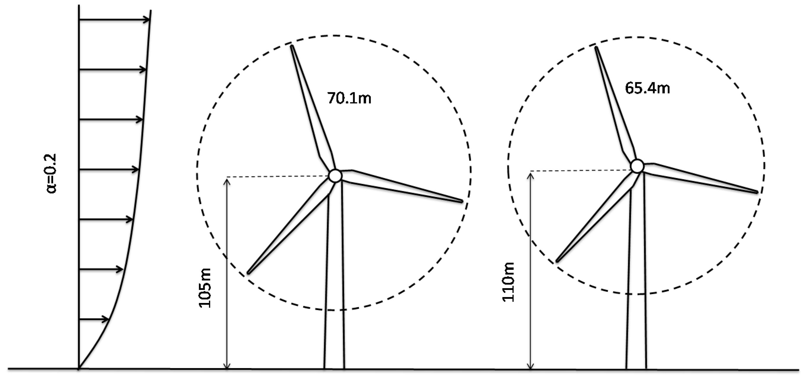
Interestingly, we observed that a lower tower is a better match for the larger rotor in both cases. For example, NPV is optimized at a 110 m tower height for a 65.4 m blade rotor, but at a 105 m tower for a 70.1 m blade rotor, as shown in Figure 21. This trend is repeated in the optimal LCoE design. Therefore, it seems from this result that, unlike the case for smaller rotor, the cost of the increase in tower height for larger wind turbine may overweight the increase in AEP due to its higher rotor thrust. The result may be influenced by the value selected for the wind shear exponent, but it is certain that more attention should be paid in upgrading the tower height of large rotors.
5. Conclusions
In this paper, a system-level optimization analysis is used to perform an integrated design of a 2 MW low wind speed turbine. Besides LCoE, the economic functions NPV, IRR and DPT are also applied as objectives in wind turbine optimization. Theoretical analysis and design results indicate that in this study IRR and DPT effect the turbine design in the same way as LCoE, all leading to a minimization of the ratio of capital expenditures to AEP. However, optimum NPV implies the largest margin between incomes and costs, resulting in a longer blade than optimum LCoE. Though more economic factors should be included to make the final decision, the optimal blade length for a certain turbine should be situated between the value of optimal LCoE and optimal NPV according to the economic analysis in this study.
The blades obtained from these economic objectives seem to be aerodynamically uncompetitive due to their larger relative thickness and smaller chord distribution compare with high Cp design. However, the sacrifice of aerodynamic performance brings significant reduction in design loads and turbine costs. This optimization shows that sometimes control of construction and maintenance costs is more crucial than optimal aerodynamics in improving the economic efficiency of wind turbines.
Further developments in this work could consider other economic metrics, such as investment size and incremental internal rate of return, to achieve more practical results. Adding modal properties, local and global buckling in the structural design constraints for the blade and tower could also be considered for future work. Finally, through a more accurate estimation of the design loads and turbine capital costs, the economic performance of a wind turbine could be more accurately evaluated.
Author Contributions
Writing-Original Draft Preparation, J.W.; Writing-Review & Editing, T.W.; Supervision, L.W. and N.Z.
Funding
This research was funded by the National Basic Research Program of China (973 Program) [grant number 2014CB046200], the National Nature science Foundation [grant number 51506089], CAS Key Laboratory of Wind Energy Utilization [grant number KLWEU-2016-0102], Jiangsu Key Laboratory of Offshore wind Turbine Blade Design and Manufacture Technology [grant number BM2016024].
Conflicts of Interest
The authors declare no conflict of interest.
References
- Johansen, J.; Madsen, H.A.; Gaunaa, M.; Bak, C.; Sørensen, N.N. Design of a wind turbine rotor for maximum aerodynamic efficiency. Wind Energy 2009, 12, 261–273. [Google Scholar] [CrossRef]
- Wang, L.; Wang, T.G.; Wu, J.H.; Chen, G.P. Multi-objective differential evolution optimization based on uniform decomposition for wind turbine blade design. Energy 2017, 120, 346–361. [Google Scholar] [CrossRef]
- Benini, E.; Toffolo, A. Optimal design of horizontal-axis wind turbines using blade-element theory and evolutionary computation. J. Sol. Energy Eng. 2002, 124, 357–363. [Google Scholar] [CrossRef]
- Maki, K.; Sbragio, R.; Vlahopoulos, N. System design of a wind turbine using a multi-level optimization approach. Renew. Energy 2012, 43, 101–110. [Google Scholar] [CrossRef]
- Chehouri, A.; Younes, R.; Ilinca, A. Review of performance optimization techniques applied to wind turbines. Appl. Energy 2015, 142, 361–388. [Google Scholar] [CrossRef]
- Ning, A.; Damiani, R.; Moriarty, P.J. Objectives and constraints for wind turbine optimization. J. Sol. Energy Eng. 2014, 136, 041010. [Google Scholar] [CrossRef]
- Savino, M.M.; Manzini, R.; Della Selva, V.; Accorsi, R. A new model for environmental and economic evaluation of renewable energy systems: The case of wind turbines. Appl. Energy 2017, 189, 739–752. [Google Scholar] [CrossRef]
- Herbert-Acero, J.F.; Probst, O.; Réthoré, P.E.; Larsen, G.C.; Castillo-Villar, K.K. A review of methodological approaches for the design and optimization of wind farms. Energies 2014, 7, 6930–7016. [Google Scholar] [CrossRef] [Green Version]
- Short, W.; Packey, D.J.; Holt, T. A Manual for the Economic Evaluation of Energy Efficiency and Renewable Energy Technologies; Technical Report NREL/TP-462-5173; National Renewable Energy Laboratory: Golden, CO, USA, 1995. [Google Scholar]
- Rodrigues, S.; Restrepo, C.; Katsouris, G.; Pinto, R.T.; Soleimanzadeh, M.; Bosman, P.; Bauer, P. A multi-objective optimization framework for offshore wind farm layouts and electric infrastructures. Energies 2016, 9, 216. [Google Scholar] [CrossRef]
- Mirghaed, M.R.; Roshandel, R. Site specific optimization of wind turbines energy cost: Iterative approach. Energy Convers. Manag. 2013, 73, 167–175. [Google Scholar] [CrossRef]
- Ashuri, T.; Zaaijer, M.B.; Martins, J.R.; van Bussel, G.J.; van Kuik, G.A. Multidisciplinary design optimization of offshore wind turbines for minimum levelized cost of energy. Renew. Energy 2014, 68, 893–905. [Google Scholar] [CrossRef] [Green Version]
- Sun, Z.Y.; Sessarego, M.; Chen, J.; Shen, W.Z. Design of the OffWindChina 5MW Wind Turbine Rotor. Energies 2017, 10, 777. [Google Scholar] [CrossRef]
- Fuglsang, P.; Madsen, H.A. Optimization method for wind turbine rotors. J. Wind Eng. Ind. Aerodyn. 1999, 80, 191–206. [Google Scholar] [CrossRef]
- Dykes, K.; Platt, A.; Guo, Y.; Ning, A.; King, R.; Parsons, T.; Petch, D.; Veers, P. Effect of Tip-Speed Constraints on the Optimized Design of a Wind Turbine; Technical Report NREL/TP-5000-61726; National Renewable Energy Laboratory: Golden, CO, USA, 2014. [Google Scholar]
- Ning, A.; Petch, D. Integrated design of downwind land-based wind turbines using analytic gradients. Wind Energy 2016, 19, 2137–2152. [Google Scholar] [CrossRef]
- Ashuri, T.; Zaaijer, M.B.; Martins, J.R.; Zhang, J. Multidisciplinary design optimization of large wind turbines—Technical, economic, and design challenges. Energy Convers. Manag. 2016, 123, 56–70. [Google Scholar] [CrossRef]
- Fuglsang, P.; Bak, C.; Schepers, J.G.; Bulder, B.; Cockerill, T.T.; Claiden, P.; Olesen, A.; van Rossen, R. Site-specific Design Optimization of Wind Turbines. Wind Energy 2002, 5, 261–279. [Google Scholar] [CrossRef]
- Hansen, M.O.L. Aerodynamics of Wind Turbines, 2nd ed.; Earthscan: London, UK, 2008. [Google Scholar]
- International Electrotechnical Committee IEC 61400-1: Wind turbines Part 1: Design Requirements, 3rd ed.; IEC: Geneva, Switzerland, 2005.
- Guo, Y.; Parsons, T.; King, R.; Dykes, K.; Veers, P. An Analytical Formulation for Sizing and Estimating the Dimensions and Weight of Wind Turbine Hub and Drivetrain Components; Technical Report NREL/TP-5000-63008; National Renewable Energy Laboratory: Golden, CO, USA, 2015. [Google Scholar]
- Díaz, G.; Gómez-Aleixandre, J.; Coto, J. Dynamic evaluation of the levelized cost of wind power generation. Energy Convers. Manag. 2015, 101, 721–729. [Google Scholar] [CrossRef]
- Tang, S.L.; Tang, H.G. The variable financial indicator IRR and the constant economic indicator NPV. Eng. Econ. 2003, 48, 69–78. [Google Scholar] [CrossRef]
- Timmer, W.A.; van Rooij, R.P.J.O.M. Summary of the Delft University wind turbine dedicated airfoils. J. Sol. Energy Eng. Trans. ASME 2003, 125, 488–496. [Google Scholar] [CrossRef]
- Ning, A.; Dykes, K. Understanding the benefits and limitations of increasing maximum rotor tip speed for utility-scale wind turbines. J. Phys. Conf. Ser. 2014, 524, 012087. [Google Scholar] [CrossRef]
- Diveux, T.; Sebastian, P.; Bernard, D.; Puiggali, J.R.; Grandidier, J.Y. Horizontal axis wind turbine systems: Optimization using genetic algorithms. Wind Energy 2001, 4, 151–171. [Google Scholar] [CrossRef]
- Gao, X.; Yang, H.; Lu, L. Optimization of wind turbine layout position in a wind farm using a newly-developed two-dimensional wake model. Appl. Energy 2016, 174, 192–200. [Google Scholar] [CrossRef]
- Gentils, T.; Wang, L.; Kolios, A. Integrated structural optimisation of offshore wind turbine support structures based on finite element analysis and genetic algorithm. Appl. Energy 2017, 199, 187–204. [Google Scholar] [CrossRef]
- Zhang, J.J.; Xu, L.W.; Gao, R.Z. Multi-island Genetic Algorithm Optimization of Suspension System. Telkomnika 2012, 10, 1685–1691. [Google Scholar] [CrossRef]
- China Wind Energy Association. China Wind Power Industry Map 2017; CWEA: Beijing, China, 2018. [Google Scholar]
- Global Wind Energy Council. Global Wind Report; GWEC: Brussels, Belgium, 2018. [Google Scholar]
- Abdulrahman, M.; Wood, D. Investigating the Power-COE trade-off for wind farm layout optimization considering commercial turbine selection and hub height variation. Renew. Energy 2017, 102, 267–278. [Google Scholar] [CrossRef]
- Alam, M.M.; Rehman, S.; Meyer, J.P.; Al-Hadhrami, L.M. Review of 600–2500 kW sized wind turbines and optimization of hub height for maximum wind energy yield realization. Renew. Sustain. Energy Rev. 2011, 15, 3839–3849. [Google Scholar] [CrossRef]
Figure 1.
Blade root flap-wise moments of SLC and full DLC calculations.

Figure 2.
Design variables of blade geometry. (a) Chord distribution; (b) Twist distribution.

Figure 3.
Flow chart of the optimization methodology.

Figure 4.
Equivalent full-loaded hours against blade length.

Figure 5.
Initial capital cost against blade length.

Figure 6.
Blade root Mf against blade length.

Figure 7.
Blade mass against blade length.

Figure 8.
Hub Mx against blade length.

Figure 9.
Gearbox mass against blade length.

Figure 10.
Mainshaft mass against blade length.

Figure 11.
Bed-plate mass against blade length.

Figure 12.
LCoE against blade length.

Figure 13.
NPV against blade length.

Figure 14.
IRR against blade length.

Figure 15.
DPT against blade length.

Figure 16.
Total discounted incomes against total discounted costs.

Figure 17.
Design results of optimum NPV and optimum LCoE.

Figure 18.
Comparison between Optimum LCoE, High Cp and Commercial 58 m blade. (a) Chord/R distribution; (b) Relative thickness distribution; (c) Thickness/R distribution.
Figure 18.
Comparison between Optimum LCoE, High Cp and Commercial 58 m blade. (a) Chord/R distribution; (b) Relative thickness distribution; (c) Thickness/R distribution.


Figure 19.
LCoE against tower height.

Figure 20.
NPV against tower height.

Figure 21.
Optimal tower heights of different rotors.


Table 1.
Static conditions for load estimation.
| Static Load Cases | Wind Speed (m/s) | Rotor Speed (rpm) | Pitch Angle (deg) | Yaw Angle (deg) | Azimuth Angle (deg) |
|---|---|---|---|---|---|
| SLC 1.1 | Vr + 3σ | 1.1 ωr | 0~10 | −8~+8 | 0~90 |
| SLC 1.2 | Vout + 3σ | ωr | 10~20 | −8~+8 | 0~90 |
| SLC 2.1 | Ve1 | 0 | 90 | 90,270 | 0 |
| SLC 2.2 | Ve50 | 0 | 90 | 30,330 | 0 |
Note: Vr: rated wind speed; Vout: cut-out wind speed; : standard deviation of the wind speed, relates to short term turbulence; ωr: rated rotor speed; Ve1: 10-min average extreme wind speed with a recurrence period of 1 year; Ve50: 10-min average extreme wind speed with a recurrence period of 50 years.
Table 2.
Economic functions for the wind turbine optimization problem.
| Function | Equation | Parameters |
|---|---|---|
| LCoE ($/kWh) | —annuity factor , r—interest rate, n—wind farm lifetime | |
| NPV ($) | —market energy price | |
| IRR (%) | —interest rate that zeroes the NPV equation | |
| DPT (years) |
Table 3.
Airfoil family.
| Airfoil Name | t/c Ratio |
|---|---|
| DU99-W-405 | 40% |
| DU99-W-350 | 35% |
| DU97-W-300 | 30% |
| DU91-W2-250 | 25% |
| DU93-W-210 | 21% |
| NACA 64-618 | 18% |
Table 4.
Main parameters of MIGA.
| Item | Value |
|---|---|
| Sub-Population Size | 10 |
| Number of Islands | 5 |
| Number of Generations | 150 |
| Rate of Crossover | 0.8 |
| Rate of Mutation | 0.01 |
| Rate of Migration | 0.3 |
| Interval of Migration | 5 |
Table 5.
Turbine properties of designs produced for optimum NPV, LCoE and Cp.
| Design Results | Blade Length (m) | Cp (-) | Capacity Factor (-) | Blade Root Mf (Nm) | Blade Mass (kg) | Hub Fx (Nm) |
|---|---|---|---|---|---|---|
| Optimum NPV | 70.1 | 0.463 | 0.342 | 1.58 × 10⁷ | 17,930 | 7.44 × 10⁵ |
| Optimum LCoE | 65.4 | 0.457 | 0.312 | 1.27 × 10⁷ | 14,552 | 6.80 × 10⁵ |
| High Cp | 65.4 | 0.487 | 0.321 | 1.40 × 10⁷ | 17,303 | 8.63 × 10⁵ |
| Design Results | Tower Height (m) | Tower Mass (tonne) | CAPEX (1000 $) | LCoE (cents/kWh) | NVP (1000 $) | |
| Optimum NPV | 105 | 369 | 2725 | 6.62 | 1295 | |
| Optimum LCoE | 93 | 270 | 2377 | 6.54 | 1223 | |
| High Cp | 93 | 346 | 2625 | 6.84 | 1096 |
© 2018 by the authors. Licensee MDPI, Basel, Switzerland. This article is an open access article distributed under the terms and conditions of the Creative Commons Attribution (CC BY) license (http://creativecommons.org/licenses/by/4.0/).
Share and Cite
MDPI and ACS Style
Wu, J.; Wang, T.; Wang, L.; Zhao, N. Impact of Economic Indicators on the Integrated Design of Wind Turbine Systems. Appl. Sci. 2018, 8, 1668. https://0-doi-org.brum.beds.ac.uk/10.3390/app8091668
AMA Style
Wu J, Wang T, Wang L, Zhao N. Impact of Economic Indicators on the Integrated Design of Wind Turbine Systems. Applied Sciences. 2018; 8(9):1668. https://0-doi-org.brum.beds.ac.uk/10.3390/app8091668
Chicago/Turabian StyleWu, Jianghai, Tongguang Wang, Long Wang, and Ning Zhao. 2018. "Impact of Economic Indicators on the Integrated Design of Wind Turbine Systems" Applied Sciences 8, no. 9: 1668. https://0-doi-org.brum.beds.ac.uk/10.3390/app8091668
Note that from the first issue of 2016, this journal uses article numbers instead of page numbers. See further details here.