Identification of Long-Range Transport Pathways and Potential Source Regions of PM2.5 and PM10 at Akedala Station, Central Asia


Institute of Desert Meteorology, China Meteorological Administration, Urumqi 830002, China
*
Authors to whom correspondence should be addressed.
Atmosphere 2020, 11(11), 1183; https://0-doi-org.brum.beds.ac.uk/10.3390/atmos11111183
Submission received: 12 September 2020
/
Revised: 24 October 2020
/
Accepted: 26 October 2020
/
Published: 2 November 2020
(This article belongs to the Section Aerosols)
Abstract
:Cluster analyses, potential source contribution function (PSCF) and concentration-weight trajectory (CWT) were used to identify the main transport pathways and potential source regions with hourly PM2.5 and PM10 concentrations in different seasons from January 2017 to December 2019 at Akedala Station, located in northwest China (Central Asia). The annual mean concentrations of PM2.5 and PM10 were 11.63 ± 9.31 and 19.99 ± 14.39 µg/m3, respectively. The air pollution was most polluted in winter, and the dominant part of PM10 (between 54 to 76%) constituted PM2.5 aerosols in Akedala. Particulate pollution in Akedala can be traced back to eastern Kazakhstan, northern Xinjiang, and western Mongolia. The cluster analyses showed that the Akedala atmosphere was mainly affected by air masses transported from the northwest. The PM2.5 and PM10 mainly came with air masses from the central and eastern regions of Kazakhstan, which are characterized by highly industrialized and semi-arid desert areas. In addition, the analyses of the pressure profile of back-trajectories showed that air mass distribution were mainly distributed above 840 hPa. This indicates that PM2.5 and PM10 concentrations were strongly affected by high altitude air masses. According to the results of the PSCF and CWT methods, the main potential source areas of PM2.5 were very similar to those of PM10. In winter and autumn, the main potential source areas with high weighted PSCF values were located in the eastern regions of Kazakhstan, northern Xinjiang, and western Mongolia. These areas contributed the highest PM2.5 concentrations from 25 to 40 µg/m3 and PM10 concentrations from 30 to 60 µg/m3 in these seasons. In spring and summer, the potential source areas with the high weighted PSCF values were distributed in eastern Kazakhstan, northern Xinjiang, the border between northeast Kazakhstan, and southern Russia. These areas contributed the highest PM2.5 concentrations from 10 to 20 µg/m3 and PM10 concentrations from 20 to 60 µg/m3 in these seasons.
1. Introduction
With the deterioration of air quality, the environmental effects of particulate matter (PM) have become one of the leading scientific issues in global climate change and ecosystems in the past few decades [1,2,3,4,5]. Many studies have concluded that PM2.5 (PM with an aerodynamic diameter less than or equal to 2.5 µm) and PM10 (PM with an aerodynamic diameter less than or equal to 10 µm) are important pollutants directly emitted into the atmosphere from anthropogenic and natural sources or are formed from secondary processes [6,7,8], which may severely affect human health at the surface level. Huang et al. [9] pointed out that sensitive groups are at the most risk. Many researchers have studied that local atmospheric circulation and monsoon affect not only the accumulation and deposition of atmospheric particles, but also the atmospheric environment in other regions through cross regional transport and source regions [10,11,12,13]. Desert dust, which is of natural origin, can be spread over long distances by the upper airflow, which impacts air quality over a wide range from arid and semi-arid regions [14]. In one study, PM10 emitted into the air in desert areas from North Africa affected not only the atmospheric environment of Central Spain, but the whole Iberian Peninsula, other parts of Europe, and even America [15,16].
Hybrid single-particle Lagrangian integrated trajectory (HYSPLIT) is a powerful tool for establishing the spatial domain of air parcels arriving at the receptor points [17,18,19,20,21]. Statistical methods such as cluster analysis, potential source contribution function (PSCF), and concentration-weight trajectory (CWT) methods have been widely used to identify the pathways and sources of air pollution [22,23,24,25,26,27,28]. Rodriguez et al. [29] pointed out that desert dust is very frequently mixed with particulate pollutants in the Saharan air layer. Gama et al. [30] used HYSPLIT, chemical transport models, and observations to show the contribution of desert dust to PM levels in Cape Verde. Typical monsoon climate plays an important role in aerosol transport, which can be verified by backward trajectory clustering [31]. Cabello and co-authors [32] pointed out that the statistical analysis of the backward trajectories by different methods confirmed that many industrial areas in Europe and north Africa as well as natural areas such as deserts have affected the mass concentration levels of particulate matter in southern Spain. A similar analysis was performed by Zhu et al. [33] based on backward trajectories, and they held that both natural sources of dust and anthropogenic sources had significant impacts on the high concentrations of PM10 in Beijing. Xin et al. [34] used PSCF and CWT methods to identify the potential sources of PM10 in the Tibetan Plateau uplift area, and revealed that eastern Xinjiang, border areas between Gansu and Inner Mongolia, and southern Tibet in China were the dominant potential sources.
Akedala, located in Central Asia, is a sensitive and fragile zone of climate change. Even the slightest air pollution may cause serious environmental impact. However up until now, little research has been conducted on the particulate matter source of origin in this region. The purpose of this paper was to reveal the transport pathways and potential sources of PM2.5 and PM10 at Akedala Station in northwest China. We used cluster analyses and the pressure profiles of backward trajectories to identify the major air mass transport pathways in the horizontal and vertical directions. We also identified the main potential source regions of PM2.5 and PM10 at Akedala Station in different seasons from January 2017 to December 2019, combining hourly PM2.5 and PM10 concentrations using the PSCF and CWT methods.
2. Material and Methods
2.1. Study Location and Data
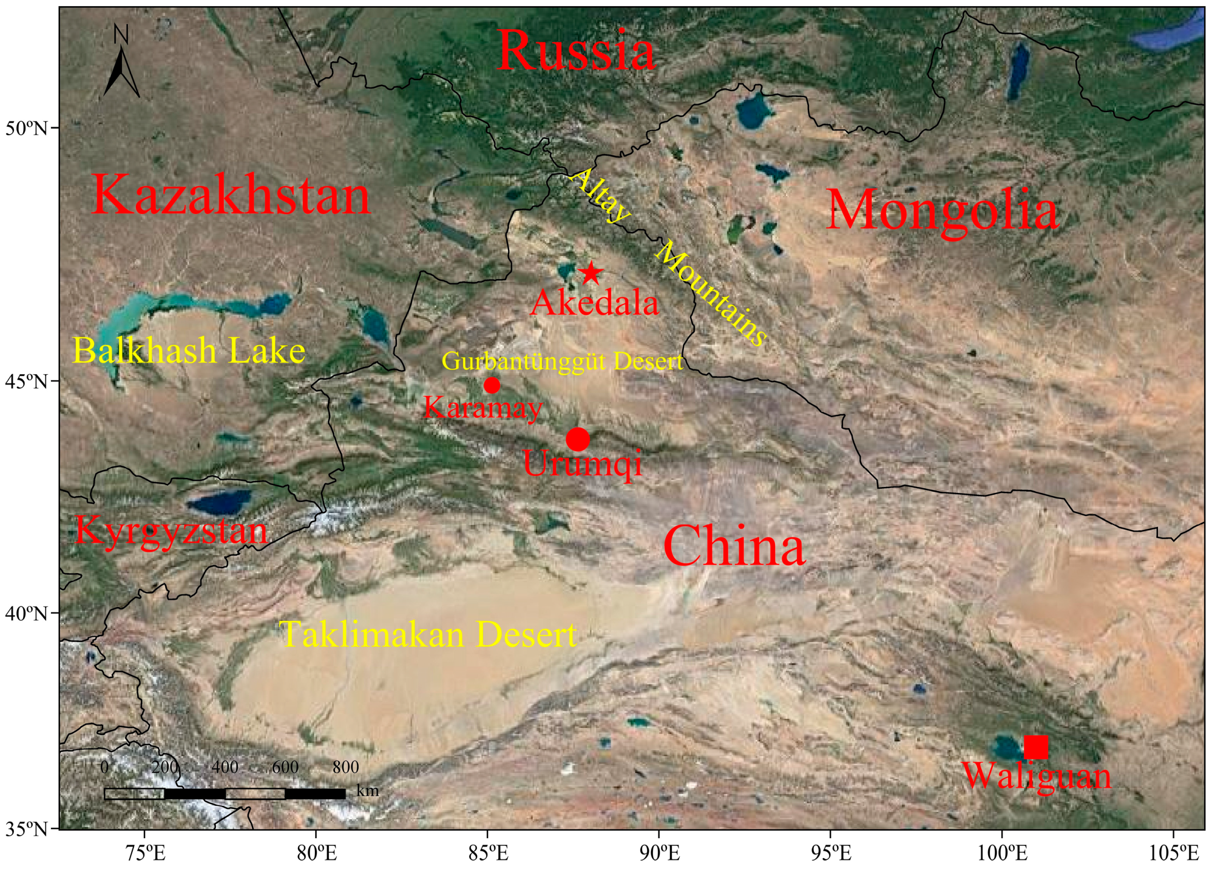
Akedala Station is located in the uppermost stream of the westerly belt in northwest China, and is under the influence of typical continental temperate arid and semi-arid climate (Figure 1) [35,36]. These atmospheric background parameters not only represent the background conditions of Xinjiang, but also represent the background conditions of Europe and Russia. The temperature, total precipitation, and average wind speed were the lowest in winter (January, February, and December), and the average wind speed was highest in spring (March, April, and May) [37]. The temperature and precipitation were highest in summer (June, July and August), and the weather parameters in autumn (September, October and November) were similar to those in spring (Table 1).
The hourly PM2.5 and PM10 concentration measurements were taken from 1 January 2017 to 31 December 2019 on Akedala station (47.10° N, 87.58° E, 562 m), which is one of the seven Chinese Global Atmosphere Watch (GAW) stations [38]. The online atmospheric dust particle monitor was the 180-E produced by Grimm in Germany, which can monitor the mass concentrations of PM10 and PM2.5 in the atmosphere online and the number concentration of 31 channels is in the range of 0.25~32 um. The injection flow rate is 1.2 L/min ± 5%, and the storage interval is 1 min~1 h. In this study, the hourly data of PM10 and PM2.5 were calculated from 5-min averages. Since there is no available observational chemical datasets, we only analyzed the mass concentration and possible pollution sources of the particulate matter at Akedala Station. The airflow trajectory meteorological reanalysis data were obtained from the Global Data Assimilation System provided by the American National Centers for Environmental Prediction (available at ftp://arlftp.arlhq.noaa.gov/pub/archives/gdas1/) [12].
2.2. Hybrid Single-Particle Lagrangian Integrated Trajectory (HYSPLIT) Model
The HYSPLIT model is a professional system jointly developed by the United States National Oceanic and Atmospheric Administration and Bureau of Meteorology Australia for calculating and analyzing atmospheric pollutant transport and diffusion trajectories [17,18,19]. This model is a comprehensive system for computing airflow trajectories, diffusion, chemical transformation, deposition simulations, and different types of pollutant emission sources [20,21,22,23].
In this study, the HYSPLIT model was used to calculate the 48-h backward trajectories from the ground, 500 m every hour (00:00–23:00 UTC) from 1 January 2017 to 31 December 2019 arriving at Akedala Station. The simulated height was selected as 500 m because the 500 m near-layer wind speed can reflect the average flow field characteristics of the boundary layer, and then reflect the characteristics of near-layer gas mass transport [39].
2.3. Trajectory Clustering
Cluster analysis is used to merge all the air mass trajectories that reach the simulated receiving point. This method can intuitively determine the source and transmission distance of the dominant air mass at different time points of the final destination point [40]. To study the source of the particulate matter at the site, TrajStat software (Version 2.0 and provided by Wang et al. Beijing, China) [41] combined with the HYSPLIT model and a geographic information system was used to calculate the backward trajectory clustering (http://www.meteothink.org/) [41]. Angle distance and Euclidean distance are two clustering methods in TrajStat software. Euclidean distance is used to define the latitude and longitude positions as variables of the distance between two trajectories. The main disadvantage of using the Euclidean distance is that if two back-trajectories that follow the same path but one has a higher speed, they are classified in two different clusters. In this study, we chose to use the angle distance instead of the Euclidean distance, mainly because our intention was to use the trajectories to determine the direction from which the air masses that reached the site had originated. More details of the angle distance method are described in Sirois and Bottenheim [42].
2.4. Potential Source Contribution Function (PSCF) Method
The potential source contribution function (PSCF) method has been widely used to identify potential source areas of pollution, which is a qualitative method based on the conditional probability function of the HYSPLIT model [17,18,19]. To calculate the PSCF, the whole geographic region covered by the trajectories is divided into an array of grid cells whose size is dependent on the domain of the back trajectories. The formula of PSCF is defined by Moody and Galloway [43] as:
where mij is the number of trajectory endpoints passing through the grid cell and nij is the total number of trajectory endpoints for which the measured pollutant concentration exceeds a threshold value selected for this pollutant in the same grid cell. The pollution levels of PM2.5 and PM10 were not the same in different seasons, so these values for PM2.5 and PM10 were defined as the averages for different seasons (Table 2) during the study period, as generally used by other receptor simulation studies [25,26,44]. As PSCF is a conditional probability, an arbitrary weight function Wij needs to be introduced to reduce the uncertainty of PSCF [20,21,22,23]. The definition of weight is as follows:
when nij in a grid is less than three times the number of average trajectory endpoints in each grid in the study area; Wij is multiplied by PSCFij, therefore, the WPSCF (weighted potential source contribution function) is expressed as:
PSCFij = mij/nij
WPSCFij = Wij × PSCFij
2.5. Concentration-Weight Trajectory (CWT) Method
The PSCF method tends to give good angular resolution, but poor radial resolution because the trajectories converge as they approach the final destination point [24,25,26,27,28]. The method combining concentrations developed by Seibert et al. [45] calculates the geometric mean concentration of each grid cell, which is then weighted by the residence time. Therefore, in this paper, the CWT method was used to calculate the concentration weight of the potential source of air masses; Stohl [46] refined this method by redistributing the concentration fields, and Hsu et al. [25] further refined it into a CWT method. The formula for CWT is as follows:
where CWTij is the average weight concentration of grid i; Cij is the average weighted concentration in the ijth cell; l is the index of the trajectory; M is the total number of trajectories; Cl is the mass concentration of the pollutant when the trajectory passes through the grid (i, j); and is the time that trajectory l stays on the grid (corresponding to the number of trajectory endpoints passing through the grid). The empirical weight function Wij for the PSCF can also be used in the CWT method to reduce the error caused by fewer nij. Therefore, the WCWT (weighted concentration-weight trajectory) is expressed as:
WCWTij = Wij × CWTij
3. Results and Discussions
3.1. Variation in PM10 and PM2.5 Concentrations
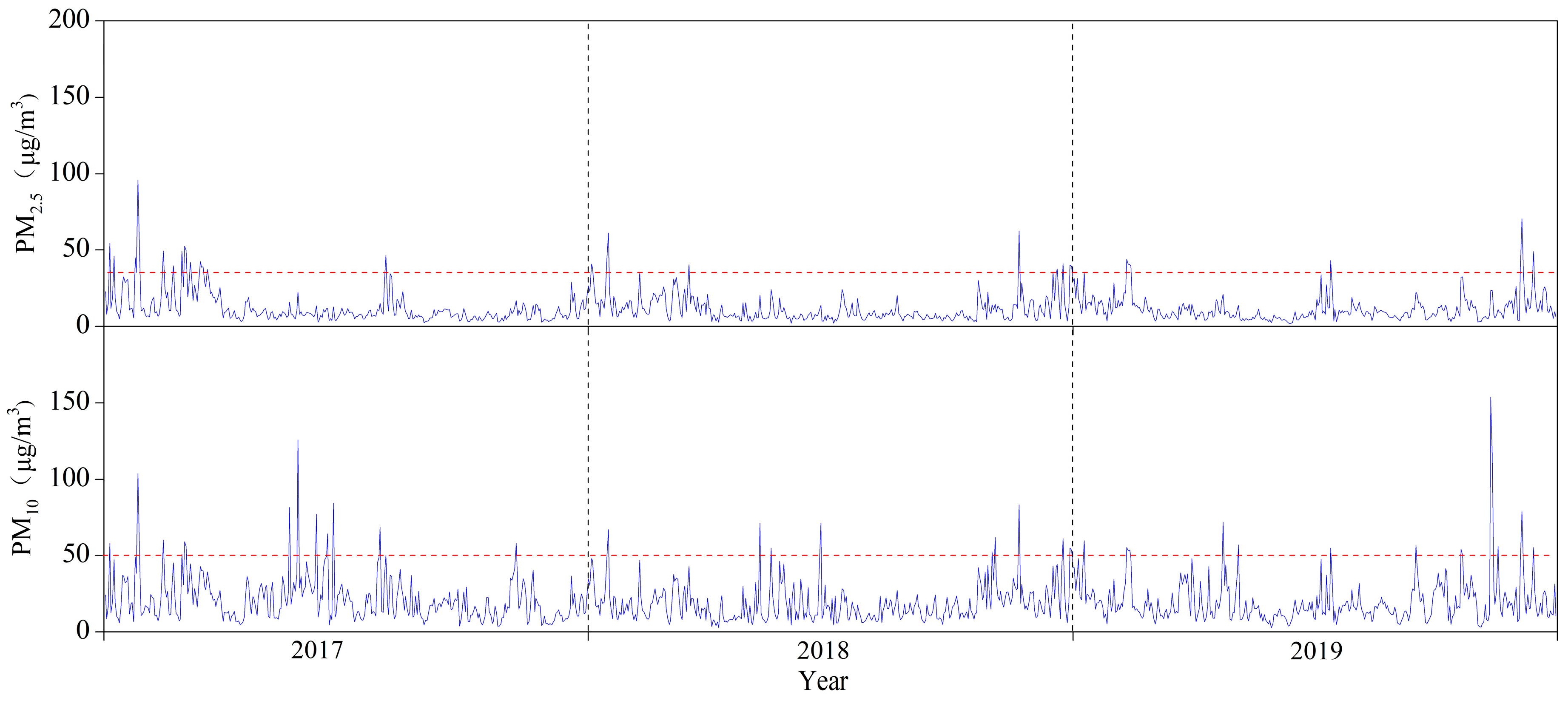
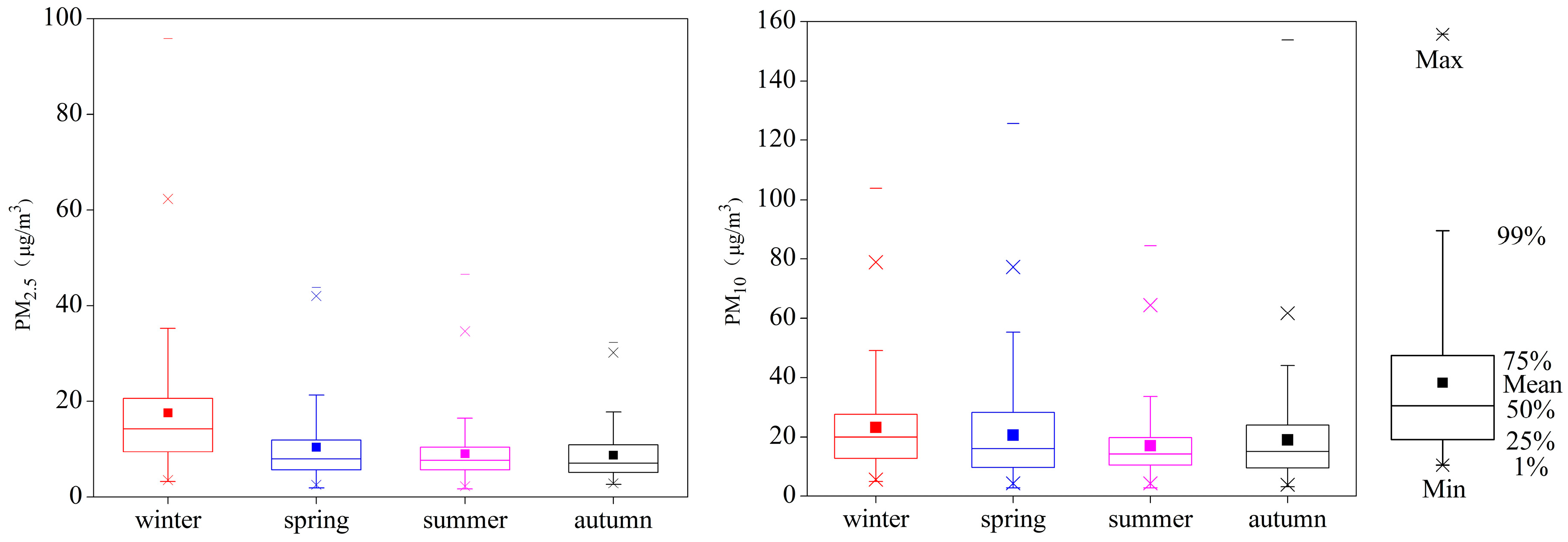
Daily mean of PM10 and PM2.5 concentrations from January 2017 to December 2019 is shown in Figure 2, and the seasonal mean concentrations of PM2.5 and PM10 are illustrated in Figure 3. As one of the GAW stations far away from human activities and social development, the air quality of Akedala Station was highly clean throughout the year. The annual mean concentrations of PM2.5 and PM10 were 11.63 ± 9.31 and 19.99 ± 14.39 µg/m3, respectively. These concentrations were 22.5% and 50% lower than the limit of the Class I standard of the Chinese Ambient Air Quality Standards (CAAQS, revised GB 3095-2012 of the Chinese National Air Quality Standards) [47] for PM2.5 (limiting values of 15 µg/m3) and PM10 (limiting values of 40 µg/m3) annual mean concentrations, respectively. In addition, the number of days exceeding the limit of the Class I standard of the CAAQS [47] was 38 days for PM2.5 (limiting values of 35 µg/m3) and 39 days for PM10 (limiting values of 50 µg/m3) daily mean concentrations, and those days accounted for the 7.7% contribution to PM mean values. However, we noted that the concentrations of PM2.5 and PM10 measured in Akedala varied significantly depending on the season, and the highest average mass concentrations of PM2.5 and PM10 were mainly observed in the winter (Table 2). Another interesting finding is that the air quality of Waliguan Station, as one of the GAW stations also located in Central Asia (Figure 1), was also highly clean. The particulate matter at Waliguan Station comes mainly from natural sources [38]. Although it is still affected by certain anthropogenic sources, the mass concentrations of PM2.5 and PM10 at Waliguan and Akedala Stations were much lower than those at other regional (Lin’an, Shangdianzi, Jinsha, and Longfengshan) GAW stations, except for Xianggelila Station [48,49,50].
The seasonal average concentrations and the standard deviations of PM and the ratios of PM2.5/PM10 are displayed in Table 2. Analysis of Variance (ANOVA) Kruskal–Wallis was used in the data analysis (p > 0.05), and the results showed that there was no significant difference between seasons. The ratio of PM2.5/PM10 can reflect the proportion of fine particles to coarse particles in the atmosphere of a region. The concentrations of PM2.5 and PM10 in the atmosphere of Akedala were significantly correlated, and the linear regression coefficient was 0.70, indicating that the two main sources of PM2.5 and PM10 were similar. The ratio of PM2.5/PM10, derived from annual arithmetic means, was 0.62 ± 0.22, indicating that PM2.5 took a relative high portion of PM10, and PM2.5 was the major pollutant. The highest ratio of PM2.5/PM10 were generally found in winter, with a value of 0.76 ± 0.18. This indicates that in winter, the biggest problem of air pollution was by PM2.5, which is more dangerous for human health than PM10. This was related to human activities such as coal combustion increasing the emissions of PM2.5 during heating period, and the wind speed was the lowest (Table 1), indicating that the height of the boundary layer in winter is low. In addition, the stable weather with low humidity and low wind velocity is not conducive to the dispersion of pollutants [51,52].
3.2. Transport Pathways
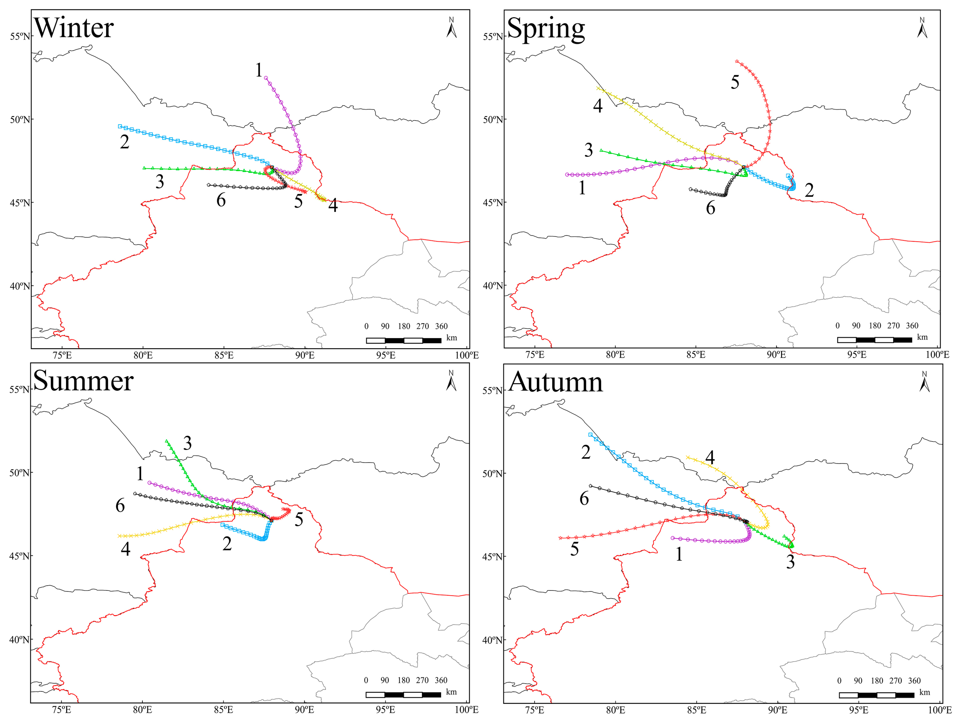
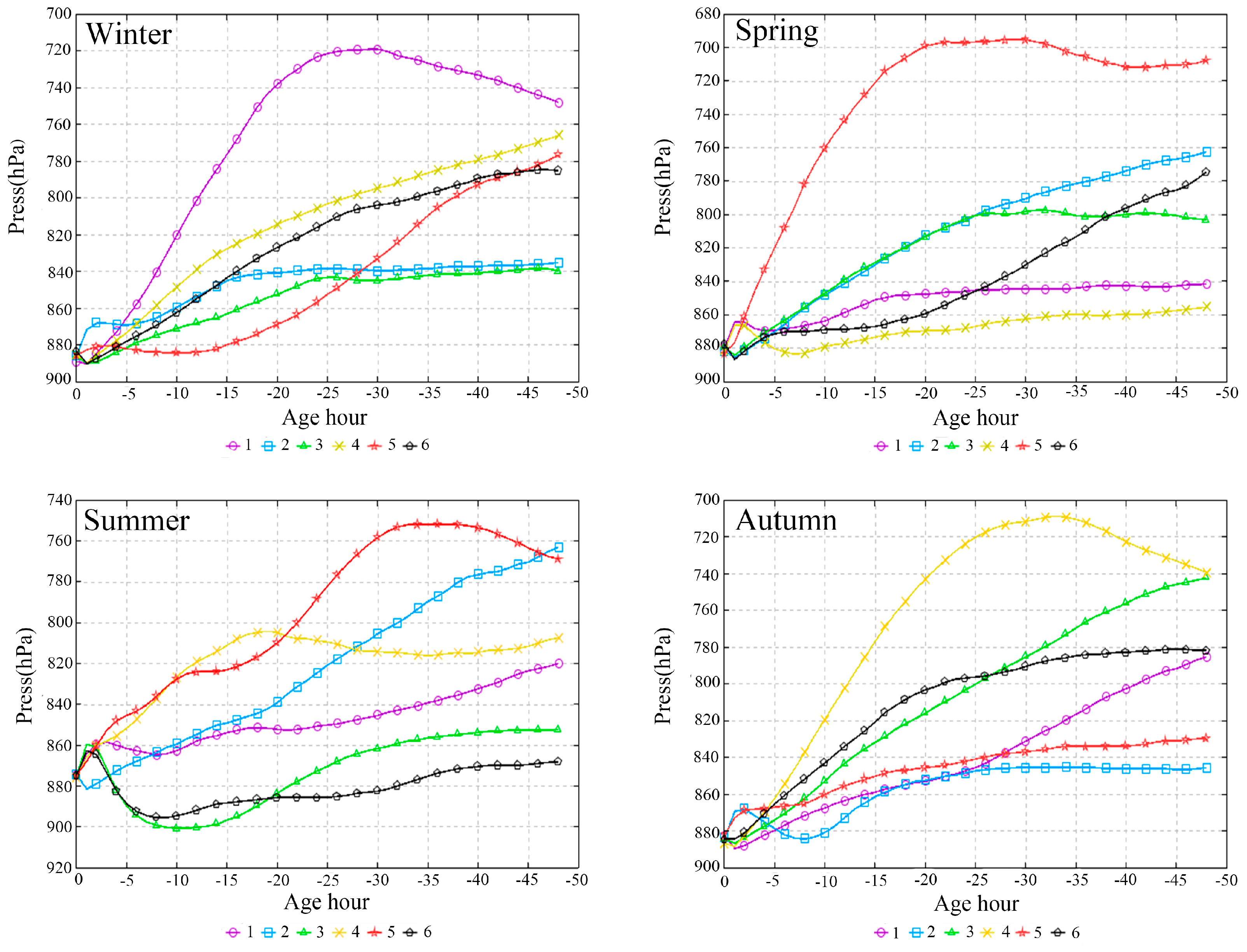
Based on the temporal and spatial distribution of backward trajectories, six major trajectory pathways were identified for each season (Figure 4), and their air pressure profiles are shown in Figure 5. Table 3 shows the numbers of trajectories assigned to each cluster, the average concentrations of PM and the standard deviations for each cluster. It can be seen from Figure 4 that across the four seasons, air masses reaching Akedala were divergent during the study period. There were obvious radial and latitudinal transport characteristics of PM2.5 and PM10 in Akedala. The average mass concentrations of PM2.5 and PM10 were the highest in winter, which was consistent with the statistical results of the observed data. The cluster analyses showed that the Akedala atmosphere was mainly affected by air masses transported from the northwest, and accounted for 32.8%, 70.2%, 95%, and 61.9% of total trajectories in winter, spring, summer, and autumn, respectively. In addition, the analyses of the pressure profile of back-trajectories showed that the air mass distribution was mainly distributed above 840 hPa (Figure 5).
In winter, the air masses of clusters 2, 3, and 5 were considered to be the major pollutant in air masses because these clusters were associated with PM2.5 and PM10 concentrations (Table 3) higher than the average concentration of winter (Table 2). The air masses associated with clusters 2, 3, and 5 accounted for about 40.3% of all trajectories. The long-distance air masses of cluster 2 and 3 started from the northwest with similar corresponding heights (1307–1559 m). These air masses passed through the highly industrialized areas in eastern Kazakhstan, known for the mining and non-ferrous metallurgy industries [53], and the west wind can transmit particulate matter over a long distance, affecting the air quality of Akedala with anthropogenic aerosol emissions. The air masses of cluster 5 varied greatly in the vertical direction (1154–2142 m), and started from the northern edge of the Gurbantünggüt Desert in northern Xinjiang [54], where it is a source of high-concentration dust aerosols. Blocked by the Altay Mountains, the air masses can easily lift the topsoil and fine sand and transmit PM over a short distance to Akedala. In addition, because of the biomass burning during the heating period, both PM2.5 and PM10 concentrations were the highest with the air masses of cluster 5 in winter [55].
In spring, the air masses associated with clusters 2 (760–885 hPa), 4 (856–885 hPa), and 6 (776–885 hPa), accounting for about 60.8% of all trajectories (Table 3), may be considered as the major pollutant air masses contributing to PM2.5 and PM10 at Akedala. Blocked by the Altay Mountains, the air masses of short-distance arc cluster 2 started from the northern Xinjiang and passed through semi-arid desert areas associated with natural aerosol emissions. The air masses of cluster 4 came from the northwest with fast moving speed along the Irtysh River, passed through the highly industrialized and semi-arid desert areas in eastern Kazakhstan, and can carry certain anthropogenic and natural contaminants onward to Akedala [53]. The air masses associated with cluster 6 traveled through industrially developed areas in Karamay city, and carried anthropogenic aerosol emissions to Akedala.
In summer, the air masses associated with clusters 1 (820–860 hPa), 3 (834–900 hPa), 4 (818–875 hPa) and 6 (865–896 hPa), with similar corresponding heights (1019–1757 m), accounting for about 95% of all trajectories (Table 3), can be considered the main air masses that have a significant influence on PM2.5 and PM10 concentrations. The concentrations of PM2.5 and PM10 carried by the air masses of clusters 1, 3, 4, and 6 were highest and the difference was small. The air masses of clusters 1, 3, 4, and 6 were all from eastern Kazakhstan, passing through Lake Balkhash. In recent years, due to the sharp drop in the water level of Lake Balkhash, the bottom of the lake had become a wasteland and a new source of sand [56]. Under the action of wind force, salt dust and sandstorms are formed, causing the dust aerosol index to continue to rise, thereby affecting the air quality of Akedala.
In autumn, the masses associated with clusters 1 (820–860 hPa), 3 (834–900 hPa), and 6 (865–896 hPa) accounted for about 37.3% of all trajectories, with higher PM2.5 and PM10 concentrations (Table 3). The distribution of the air masses in autumn was similar to those in winter and spring. The air masses associated with cluster 1 originated from northern Xinjiang and passed through desert and semi-desert regions onward to Akedala. The air masses of cyclone cluster 3 with a short track, accounting for about 16.2% of all trajectories, represented the pathway polluted by PM2.5 and PM10. Cluster 5 represents air masses that were transported from the desert areas in southeastern Kazakhstan. The air masses of cluster 6 started from central Kazakhstan, and passed through eastern Kazakhstan, which is characterized by industrial emissions and semi-arid desert areas [53]. Under the action of the monsoon, atmospheric particulate matter could be transported into Akedala from such distant sources.
3.3. PSCF Analyses
Cluster analyses provide an effective tool for studying the long-range transport pathways of pollutants. However, it has some uncertain parameters caused by subjective factors such as simulation height, the selection of the clustering algorithm, and the number of clusters. In addition, it cannot simulate the potential source regions and contribution levels of PM2.5 and PM10 pollution. In order to better understand the transportation of long-range air masses that may have an important impact on PM2.5 and PM10 concentrations in Akedala and to find their potential source regions, PSCF and CWT methods combined with backward trajectories can be used.
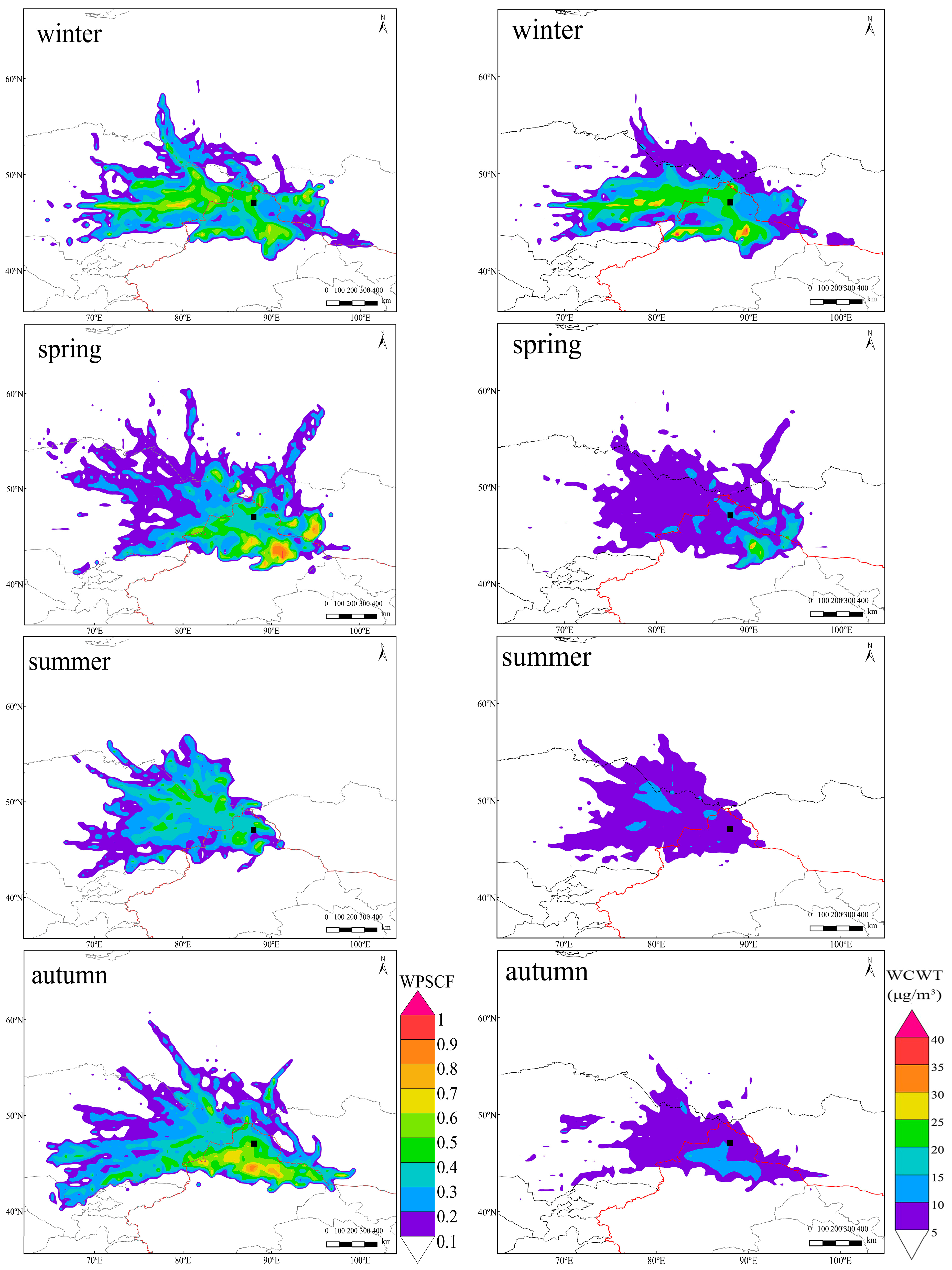
Figure 6 shows the calculation results of the WPSCF and WCWT of PM2.5 across four seasons in Akedala. WPSCF values of 0–0.3, 0.3–0.7, and 0.7–1.0 were divided into light, moderate, and severe pollution grids, respectively, to identify potential source grid attributes. The colors represent the contribution levels of potential source area and the yellow color could be associated with high PM2.5 concentrations while the blue color represents low PM2.5 concentrations. The WPSCF map distributions for different seasons were significantly different because of the differences in the air flows in different seasons.
In general, the spatial distributions of PM2.5 potential source areas were large, and the distributions of the main source areas were relatively concentrated. In winter, the main potential source areas of PM2.5, with WPSCF values of 0.4–0.8, were located in the east region of Kazakhstan, north Xinjiang, and western Mongolia. The Gobi Desert in these areas is a natural source of PM2.5. In spring, compared to winter, the main potential source areas of PM2.5 moved eastward with a narrower range, but the severe pollution source areas with high WPSCF values of 0.7–0.9 were more concentrated and had small-scale cluster distributions in northeastern Xinjiang, western Mongolia, the border between northeast Kazakhstan and southern Russia. In summer, the spatial distributions of PM2.5 were mainly light polluted grids, with low WPSCF values of 0.1–0.5, mainly distributed in eastern Kazakhstan, the Altay region in northern Xinjiang, and small distributions in southern Russia. In autumn, the severe pollution source areas of PM2.5 were concentrated in the northern part of Xinjiang, corresponding to the Gurbantünggüt desert zones in the Junggar Basin, and there were light pollution source areas in eastern Kazakhstan. Therefore, these places could be considered as the main potential source areas.
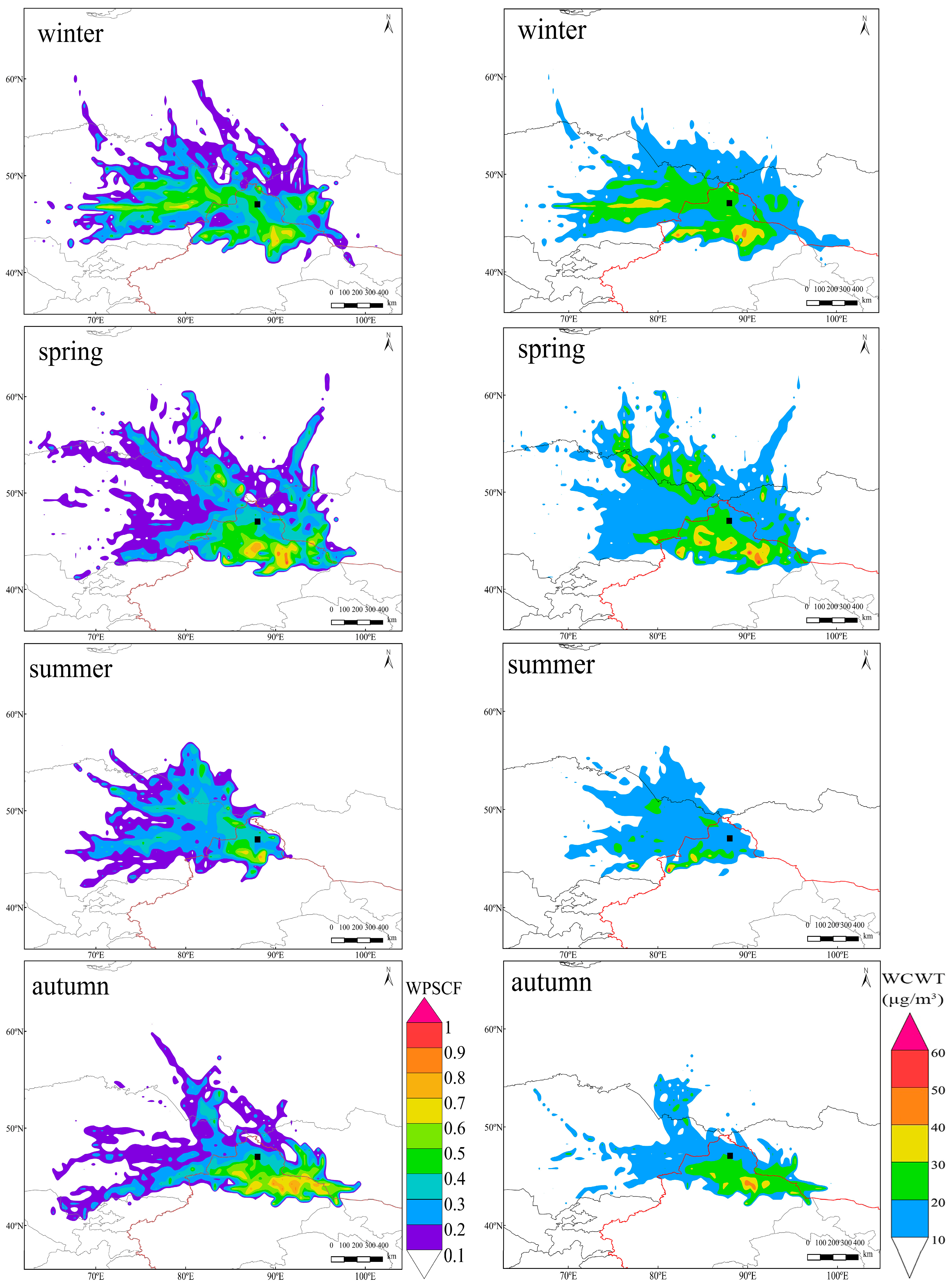
The PSCF maps covering the study period that are shown in Figure 7 were plotted in order to identify the probable locations of potential source regions contributing to PM10 levels in the four seasons in Akedala. Comparing the two maps of PM2.5 and PM10, it could be found that the main potential source regions of PM2.5 were similar to PM10. During the different seasons, the impact of potential source areas was noted in the sequence winter > spring > autumn > summer.
3.4. CWT Analyses
Potential source areas calculated by the PSCF method were the proportion of pollution trajectories in the grid, which cannot quantitatively reflect the contribution of pollutants in potential source regions. Therefore, the CWT method was used to calculate the pollution degree of different trajectories.
As shown in Figure 6, the results of PM2.5 through the CWT method were somewhat different from the results analyzed through the PSCF method. The regions with the yellow color corresponded to the main contributing sources associated with the highest PM2.5 values. In winter, the highest WCWT values covering the map were distributed in eastern Kazakhstan, northern Xinjiang, and western Mongolia. These areas were the main contributing sources to the highest PM2.5 values (exceeding 25 µg/m3), and some small areas were even higher than 40 µg/m3. In spring, the highest WCWT values were only distributed in the northeast of Xinjiang, China. These areas were the main contribution sources associated with the highest PM2.5 concentrations of 30 µg/m3. In summer and autumn, the maximum WCWT was smaller than in winter. The significant potential source regions in summer were mainly located in eastern Kazakhstan and northern Xinjiang with low WCWT values of about 5–15 µg/m3. In addition, they were also distributed at the junction of northeastern Kazakhstan and southern Russia. In autumn, the highest WCWT values in the map were distributed in northern Xinjiang with WCWT values of about 10–15 µg/m3.
Compared to Figure 7, we found that the WCWT maps of PM10 were very similar to the WCWT maps of PM2.5. In addition, the border between northeast Kazakhstan and southern Russia had the high WCWT values at about 30–50 µg/m3. The potential source areas associated with the high WCWT values for PM10 were about 30–60, 30–50, 10–30, and 30–50 µg/m3 in winter, spring, summer, and autumn, respectively.
4. Conclusions
In this paper, cluster analyses were used to identify the main transport pathways in the horizontal and vertical directions with hourly data of PM2.5, PM10 from January 2017 to December 2019 in Akedala. The PSCF and CWT methods were also applied to identify the potential source regions. The annual mean concentrations of PM2.5 and PM10 were 11.63 ± 9.31 and 19.99 ± 14.39 µg/m3, respectively. The average mass concentrations of PM2.5 and PM10 were the highest in winter. The ratios of PM2.5/PM10 were 0.76 ± 0.18, 0.58 ± 0.25, 0.57 ± 0.19, and 0.54 ± 0.2 in winter, spring, summer, and autumn, respectively. These indicated that the dominant part of PM10 (between 54 and 76%) constituted PM2.5 aerosols in Akedala.
There were clear seasonal and spatial variations of the air masses in both the horizontal and vertical directions in Akedala. Particulate pollution in Akedala can be traced back to eastern Kazakhstan, northern Xinjiang, and western Mongolia. The cluster analyses showed that the Akedala atmosphere was mainly affected by polluted air masses transported from the northwest, which accounted for 32.8%, 70.2%, 95%, and 61.9% of the total trajectories in winter, spring, summer, and autumn, respectively. These long-range air masses passed through central and eastern Kazakhstan, which is characterized by industrial emissions and semi-arid desert areas. Secondly, Akedala was affected by short-distance arc air masses from the southeast, which were blocked by Altay Mountains and moved slowly to Akedala. In addition, the results of the pressure profile of the air masses showed that the air masses with the most important influence were mainly distributed above 840 hPa, indicating that high altitude air masses had important influences on PM2.5 and PM10 concentrations in Akedala.
According to the results of the PSCF and CWT methods, the main potential source areas of PM2.5 were very similar to those of PM10. There were obvious spatial distribution characteristics and seasonal differences of the potential source areas in Akedala. In winter and autumn, the main potential source areas with high PSCF values were located in the east regions of Kazakhstan, northern Xinjiang, and western Mongolia. These areas contributed the highest PM2.5 concentrations from 25 to 40 µg/m3 and PM10 concentrations from 30 to 60 µg/m3 in these seasons. In spring and summer, the potential source areas with the highest WPSCF values were distributed in eastern Kazakhstan, north Xinjiang, the border between northeast Kazakhstan, and southern Russia. These areas contributed the highest PM2.5 concentrations from 10 to 20 µg/m3 and PM10 concentrations from 20 to 60 µg/m3 in these seasons. In the future, we will perform a case study and select a high-PM event in Akedala and zone in on that event. In addition, the effects of meteorological characteristics on PM concentrations in the Akedala area such as temperature, wind speed, and relative humidity need to be studied in detail.
Author Contributions
Conceptualization, Q.H.; Data curation, H.L. and X.L.; Formal analysis, H.L.; Funding acquisition, Q.H.; Project administration, Q.H.; Resources, Q.H.; Software, H.L.; Supervision, X.L.; Validation, X.L.; Writing—original draft, H.L.; Writing—review & editing, Q.H. All authors have read and agreed to the published version of the manuscript.
Funding
This work was supported by the Second Tibetan Plateau Scientific Expedition and Research (STEP) program (grant no. 2019QZKK010206).
Acknowledgments
The authors acknowledge Akedala Station and the NOAA for the data that they kindly provided.
Conflicts of Interest
The authors declare no conflict of interest.
References
- Heal, M.R.; Kumar, P.; Harrison, R.M. Particles, air quality, policy and health. Chem. Soc. Rev. 2012, 41, 6606–6630. [Google Scholar] [CrossRef] [PubMed] [Green Version]
- Timonen, K.L.; Vanninen, E.; de Hartog, J.; Ibald-Mulli, A.; Brunekreef, B.; Gold, D.R.; Heinrich, J.; Hoek, G.; Lanki, T.; Peters, A.; et al. Effects of ultrafine and fine particulate and gaseous air pollution on cardiac autonomic control in subjects with coronary artery disease: The ULTRA study. J. Expo. Sci. Environ. Epidemiol. 2006, 16, 332–341. [Google Scholar] [CrossRef] [PubMed] [Green Version]
- Cyrys, J.; Heinrich, J.; Hoek, G.; Meliefste, K.; Lewne, M.; Gehring, U.; Bellander, T.; Fischer, P.; van Vliet, P.; Brauer, M.; et al. Comparison between different traffic-related particle indicators: Elemental carbon (EC), PM2.5 mass, and absorbance. J. Expo. Anal. Environ. Epidemiol. 2003, 13, 134–143. [Google Scholar] [CrossRef] [PubMed] [Green Version]
- Wallace, L.; Ott, W. Personal exposure to ultrafine particles. J. Expo. Sci. Environ. Epidemiol. 2011, 21, 20–30. [Google Scholar] [CrossRef] [PubMed]
- Xu, X.; Jiang, Z.; Li, J.; Chu, Y.; Tan, W.; Li, C. Impacts of meteorology and emission control on the abnormally low particulate matter concentration observed during the winter of 2017. Atmos. Environ. 2020, 225, 117377. [Google Scholar] [CrossRef]
- Wan Mahiyuddin, W.R.; Sahani, M.; Aripin, R.; Latif, M.T.; Thach, T.-Q.; Wong, C.-M. Short-term effects of daily air pollution on mortality. Atmos. Environ. 2013, 65, 69–79. [Google Scholar] [CrossRef]
- Kelly, F.J.; Fussell, J.C. Air pollution and public health: Emerging hazards and improved understanding of risk. Environ. Geochem. Health 2015, 37, 631–649. [Google Scholar] [CrossRef] [Green Version]
- Feng, R.; Zheng, H.-J. Evidence for regional heterogeneous atmospheric particulate matter distribution in China: Implications for air pollution control. Environ. Chem. Lett. 2019, 17, 1839–1847. [Google Scholar] [CrossRef]
- Huang, K.; Yang, X.; Liang, F.; Liu, F.; Li, J.; Xiao, Q.; Chen, J.; Liu, X.; Cao, J.; Shen, C.; et al. Long-term exposure to fine particulate matter and hypertension incidence in China. Hypertension 2019, 73, 1195–1201. [Google Scholar] [CrossRef]
- Volná, V.; Hladký, D. Detailed assessment of the effects of meteorological conditions on PM10 concentrations in the northeastern part of the Czech Republic. Atmosphere 2020, 11, 497. [Google Scholar] [CrossRef]
- Challa, V.S.; Indrcanti, J.; Baham, J.M.; Patrick, C.; Rabarison, M.K.; Young, J.H.; Hughes, R.; Swanier, S.J.; Hardy, M.G.; Yerramilli, A. Sensitivity of atmospheric dispersion simulations by HYSPLIT to the meteorological predictions from a meso-scale model. Environ. Fluid. Mech. 2008, 8, 367–387. [Google Scholar] [CrossRef]
- Li, D.; Liu, J.; Zhang, J.; Gui, H.; Du, P.; Yu, T.; Wang, J.; Lu, Y.; Liu, W.; Cheng, Y. Identification of long-range transport pathways and potential sources of PM2.5 and PM10 in Beijing from 2014 to 2015. J. Environ. Sci. (China) 2017, 56, 214–229. [Google Scholar] [CrossRef] [PubMed]
- Xiao, C.; Chang, M.; Guo, P.; Gu, M.; Li, Y. Analysis of air quality characteristics of Beijing-Tianjin-Hebei and its surrounding air pollution transport channel cities in China. J. Environ. Sci. (China). 2020, 87, 213–227. [Google Scholar] [CrossRef]
- Huneeus, N.; Schulz, M.; Balkanski, Y.; Griesfeller, J.; Prospero, J.; Kinne, S.; Bauer, S.; Boucher, O.; Chin, M.; Dentener, F.; et al. Global dust model intercomparison in AeroCom phase I. Atmos. Chem. Phys. 2011, 11, 7781–7816. [Google Scholar] [CrossRef] [Green Version]
- Salvador, P.; Artinano, B.; Querol, X.; Alastuey, A. A combined analysis of backward trajectories and aerosol chemistry to characterise long-range transport episodes of particulate matter: The Madrid air basin, a case study. Sci. Total Environ. 2008, 390, 495–506. [Google Scholar] [CrossRef] [PubMed]
- Querol, X.; Tobías, A.; Pérez, N.; Karanasiou, A.; Amato, F.; Stafoggia, M.; Pérez García-Pando, C.; Ginoux, P.; Forastiere, F.; Gumy, S.; et al. Monitoring the impact of desert dust outbreaks for air quality for health studies. Environ. Int. 2019, 130, 104867. [Google Scholar] [CrossRef]
- Li, C.; Dai, Z.; Liu, X.; Wu, P. Transport Pathways and Potential Source Region Contributions of PM2.5 in Weifang: Seasonal Variations. Appl. Sci. 2020, 10, 2835. [Google Scholar] [CrossRef] [Green Version]
- Escudero, M.; Stein, A.; Draxler, R.R.; Querol, X.; Alastuey, A.; Castillo, S.; Avila, A. Determination of the contribution of northern Africa dust source areas to PM10 concentrations over the central Iberian Peninsula using the Hybrid Single-Particle Lagrangian Integrated Trajectory model (HYSPLIT) model. J. Geophys. Res. 2006, 111. [Google Scholar] [CrossRef]
- Escudero, M.; Stein, A.F.; Draxler, R.R.; Querol, X.; Alastuey, A.; Castillo, S.; Avila, A. Source apportionment for African dust outbreaks over the Western Mediterranean using the HYSPLIT model. Atmos. Res. 2011, 99, 518–527. [Google Scholar] [CrossRef]
- Shan, W.; Yin, Y.; Lu, H.; Liang, S. A meteorological analysis of ozone episodes using HYSPLIT model and surface data. Atmos. Environ. 2009, 93, 767–776. [Google Scholar] [CrossRef]
- Wang, Y.; Stein, A.F.; Draxler, R.R.; de la Rosa, J.D.; Zhang, X. Global sand and dust storms in 2008: Observation and HYSPLIT model verification. Atmos. Environ. 2011, 45, 6368–6381. [Google Scholar] [CrossRef]
- Wang, F.; Chen, D.S.; Cheng, S.Y.; Li, J.B.; Li, M.J.; Ren, Z.H. Identification of regional atmospheric PM10 transport pathways using HYSPLIT, MM5-CMAQ and synoptic pressure pattern analysis. Environ. Model. Softw. 2010, 25, 927–934. [Google Scholar] [CrossRef]
- McGowan, H.; Clark, A. Identification of dust transport pathways from Lake Eyre, Australia using Hysplit. Atmos. Environ. 2008, 42, 6915–6925. [Google Scholar] [CrossRef]
- Hu, X.; Yin, Y.; Duan, L.; Wang, H.; Song, W.; Xiu, G. Temporal and spatial variation of PM2.5 in Xining, Northeast of the Qinghai–Xizang (Tibet) Plateau. Atmosphere 2020, 11, 953. [Google Scholar] [CrossRef]
- Hsu, Y.K.; Holsen, T.M.; Hopke, P.K. Comparison of hybrid receptor models to locate PCB sources in Chicago. Atmos. Environ. 2003, 37, 545–562. [Google Scholar] [CrossRef]
- Wang, Y.Q.; Zhang, X.Y.; Arimoto, R. The contribution from distant dust sources to the atmospheric particulate matter loadings at XiAn, China during spring. Sci. Total Environ. 2006, 368, 875–883. [Google Scholar] [CrossRef]
- Hao, T.; Cai, Z.; Chen, S.; Han, S.; Yao, Q.; Fan, W. Transport pathways and potential source regions of PM2.5 on the west coast of Bohai Bay during 2009–2018. Atmosphere 2019, 10, 345. [Google Scholar] [CrossRef] [Green Version]
- Dvorská, A.; Lammel, G.; Holoubek, I. Recent trends of persistent organic pollutants in air in central Europe-Air monitoring in combination with air mass trajectory statistics as a tool to study the effectivity of regional chemical policy. Atmos. Environ. 2009, 43, 1280–1287. [Google Scholar] [CrossRef]
- Rodríguez, S.; Alastuey, A.; Alonso-Pérez, S.; Querol, X.; Cuevas, E.; Abreu-Afonso, J.; Viana, M.; Pérez, N.; Pandolfi, M.; de la Rosa, J. Transport of desert dust mixed with North African industrial pollutants in the subtropical Saharan Air Layer. Atmos. Chem. Phys. 2011, 11, 6663–6685. [Google Scholar] [CrossRef] [Green Version]
- Gama, C.; Tchepel, O.; Baldasano, J.M.; Basart, S.; Ferreira, J.; Pio, C.; Cardoso, J.; Borrego, C. Seasonal patterns of Saharan dust over Cape Verde–a combined approach using observations and modelling. Tellus B Chem. Phys. Meteo. 2015, 67, 24410. [Google Scholar] [CrossRef] [Green Version]
- Sun, X.; Luo, X.S.; Xu, J.; Zhao, Z.; Chen, Y.; Wu, L.; Chen, Q.; Zhang, D. Spatio-temporal variations and factors of a provincial PM2.5 pollution in eastern China during 2013-2017 by geostatistics. Sci. Rep. 2019, 9, 3613. [Google Scholar] [CrossRef] [Green Version]
- Cabello, M.; Orza, J.A.G.; Dueñas, C.; Liger, E.; Gordo, E.; Cañete, S. Back-trajectory analysis of African dust outbreaks at a coastal city in southern Spain: Selection of starting heights and assessment of African and concurrent Mediterranean contributions. Atmos. Environ. 2016, 140, 10–21. [Google Scholar] [CrossRef]
- Zhu, L.; Huang, X.; Shi, H.; Cai, X.; Song, Y. Transport pathways and potential sources of PM10 in Beijing. Atmos. Environ. 2011, 45, 594–604. [Google Scholar] [CrossRef]
- Xin, Y.J.; Wang, G.C.; Chen, L. Identification of long-range transport pathways and potential sources of PM10 in Tibetan Plateau uplift area: Case study of Xining, China in 2014. Aerosol Air Qual. Res. 2016, 16, 1044–1054. [Google Scholar] [CrossRef] [Green Version]
- Wang, H.; He, Q.; Liu, T.; Chen, F.; Liu, X.; Zhong, Y.; Yang, S. Characteristics and source of black carbon aerosols at Akedala station, Central Asia. Meteoro. Atmos. Phys. 2012, 118, 189–197. [Google Scholar] [CrossRef]
- Wang, H.; Ma, J.; Shen, Y.; Wang, Y. Assessment of ozone variations and meteorological influences at a rural site in Northern Xinjiang. Bull. Environ. Contam. Toxicol. 2015, 94, 240–246. [Google Scholar] [CrossRef]
- Zhang, G.; Cui, C.; Li, Y.; Li, J. Simulation on air flow 3-dimension trajectories of the boundary layer at Akedala background atmosphere station. J. Des. Res. 2008, 154–160. (In Chinese). Available online: http://en.cnki.com.cn/Article_en/CJFDTotal-ZGSS200801026.htm (accessed on 12 September 2020).
- Liu, N.; Lin, W.; Ma, J.; Xu, W.; Xu, X. Seasonal variation in surface ozone and its regional characteristics at global atmosphere watch stations in China. J. Environ. Sci. (China) 2019, 77, 291–302. [Google Scholar] [CrossRef]
- Gao, N.; Hopke, P.K.; Reid, W.N. Possible sources for some trace elements found in airborne particles and precipitation in dorset, Ontario. J. Air. Waste. Manag. Assoc. 1996, 46, 1035–1047. [Google Scholar] [CrossRef] [Green Version]
- Su, L.; Yuan, Z.; Fung, J.C.; Lau, A.K. A comparison of HYSPLIT backward trajectories generated from two GDAS datasets. Sci. Total Environ. 2015, 506–507, 527–537. [Google Scholar] [CrossRef]
- Wang, Y.Q.; Zhang, X.Y.; Draxler, R.R. TrajStat: GIS-based software that uses various trajectory statistical analysis methods to identify potential sources from long-term air pollution measurement data. Environ. Model. Softw. 2009, 24, 938–939. [Google Scholar] [CrossRef]
- Sirois, A.; Bottenheim, J.W. Use of backward trajectories to interpret the 5-year record of PAN and O3 ambient air concentrations at Kejimkujik National Park, Nova Scotia. J. Geophys. Res. Atmos. 1995, 100, 2867–2881. [Google Scholar] [CrossRef]
- Moody, J.L.; Galloway, J.N. Quantifying the relationship between atmospheric transport and the chemical composition of precipitation on Bermuda. Tellus B 1988, 40, 463–479. [Google Scholar] [CrossRef] [Green Version]
- Vellingiri, K.; Kim, K.-H.; Lim, J.-M.; Lee, J.-H.; Ma, C.-J.; Jeon, B.-H.; Sohn, J.-R.; Kumar, P.; Kang, C.-H. Identification of nitrogen dioxide and ozone source regions for an urban area in Korea using back trajectory analysis. Atmos. Res. 2016, 176–177, 212–221. [Google Scholar] [CrossRef]
- Seibert, P.; Kromp-Kolb, H.; Baltensperger, U.; Jost, D.T.; Schwikowski, M.; Kasper, A.; Puxbaum, H. Trajectory analysis of aerosol measurements at high alpine sites. In Transport and Transformation of Pollutants in the Troposphere; Borrel, P.M., Borrel, P., Cvitas, T., Seiler, W., Eds.; Academic Publishing: The Hague, The Netherlands, 1994; pp. 689–693. [Google Scholar]
- Stohl, A. Trajectory statistics-a new method to establish source-receptor relationships of air pollutants and its application to the transport of particulate sulfate in Europe. Atmos. Environ. 1996, 30, 579–587. [Google Scholar] [CrossRef]
- Environmental Protection Department, State Administration of Quality Supervision, Inspection and Quarantine. Ambient Air Quality Standards. In The State Standard of the People’s Republic of China GB; Environmental Science Press: Beijing, China, 2012. (In Chinese) [Google Scholar]
- Xue, L.K.; Wang, T.; Zhang, J.M.; Zhang, X.C.; Deliger; Poon, C.N.; Ding, A.J.; Zhou, X.H.; Wu, W.S.; Tang, J.; et al. Source of surface ozone and reactive nitrogen speciation at Mount Waliguan in western China: New insights from the 2006 summer study. J. Geophys. Res. 2011, 116. [Google Scholar] [CrossRef] [Green Version]
- Zhang, F.; Zhou, L.; Yao, B.; Zhang, X.; Xu, L.; Zhang, X.; Zhou, H.; Dong, F.; Zhou, L. In-situ measurement of atmospheric CFC-11 at the Shangdianzi Global Atmosphere Watch (GAW) Regional Station. Sci. China Earth Sci. 2010, 54, 298–304. [Google Scholar] [CrossRef]
- Qu, W.; Wang, D.; Wang, Y.; Sheng, L.; Fu, G. Seasonal variation, source, and regional representativeness of the background aerosol from two remote sites in western China. Environ. Monit. Assess. 2010, 167, 265–288. [Google Scholar] [CrossRef] [PubMed]
- Seibert, R.; Nikolova, I.; Volná, V.; Krejčí, B.; Hladký, D. Air Pollution Sources’ Contribution to PM2.5 Concentration in the Northeastern Part of the Czech Republic. Atmosphere 2020, 11, 522. [Google Scholar] [CrossRef]
- Pekney, N.J.; Davidson, C.I.; Zhou, L.; Hopke, P.K. Application of PSCF and CPF to PMF-Modeled Sources of PM2.5 in Pittsburgh. Aerosol Sci. Technol. 2006, 40, 952–961. [Google Scholar] [CrossRef] [Green Version]
- Rudoy, D.; Alimbaev, T.; Omarova, B.; Abzhapparova, B.; Ilyassova, K.; Yermagambetova, K.; Mazhitova, Z.; Ignateva, S. Environment of East Kazakhstan: State and main directions of optimization. In E3S Web of Conferences; EDP Sciences: Les Ulis, France, 2020; Volume 175. [Google Scholar] [CrossRef]
- Mamtimin, A.; Wang, Y.; Sayit, H.; Yang, X.; Yang, F.; Huo, W.; Zhou, C. Seasonal variations of the near-surface atmospheric boundary layer structure in China’s Gurbantünggüt Desert. Adv. Meteorol. 2020, 2020, 6137237. [Google Scholar] [CrossRef]
- Chen, J.; Li, C.; Ristovski, Z.; Milic, A.; Gu, Y.; Islam, M.S.; Wang, S.; Hao, J.; Zhang, H.; He, C.; et al. A review of biomass burning: Emissions and impacts on air quality, health and climate in China. Sci. Total Environ. 2017, 579, 1000–1034. [Google Scholar] [CrossRef] [PubMed] [Green Version]
- Mischke, M.; Zhang, C.; Plessen, B. Lake Balkhash (Kazakhstan): Recent human impact and natural variability in the last 2900 years. J. Great Lakes Res. 2020, 46, 267–276. [Google Scholar] [CrossRef]
Figure 1.
Location of the study area (the red star represents Akedala Station).

Figure 2.
Daily mean concentrations of PM2.5 and PM10 in Akedala station from 1 January 2017 to 31 December 2019 (the red dotted lines represent the limit of the Class I standard of CAAQS for PM2.5 and PM10 daily mean concentrations).
Figure 2.
Daily mean concentrations of PM2.5 and PM10 in Akedala station from 1 January 2017 to 31 December 2019 (the red dotted lines represent the limit of the Class I standard of CAAQS for PM2.5 and PM10 daily mean concentrations).

Figure 3.
Seasonal variations of PM2.5 and PM10 during 2017–2019. The box plots show PM2.5 and PM10 mean values, together with the maximum, the minimum, and the 99th, 75th, 50th, 25th, and 1st percentiles.
Figure 3.
Seasonal variations of PM2.5 and PM10 during 2017–2019. The box plots show PM2.5 and PM10 mean values, together with the maximum, the minimum, and the 99th, 75th, 50th, 25th, and 1st percentiles.

Figure 4.
Cluster-mean back-trajectories by using the hybrid single-particle Lagrangian integrated trajectory (HYSPLIT) model in Akedala Station from January 2017 to December 2019.
Figure 4.
Cluster-mean back-trajectories by using the hybrid single-particle Lagrangian integrated trajectory (HYSPLIT) model in Akedala Station from January 2017 to December 2019.

Figure 5.
Air pressure profiles of the backward trajectories from January 2017 to December 2019.

Figure 6.
WPSCF and WCWT maps of PM2.5 in winter, spring, summer, and autumn from January 2017 to December 2019. The black square represents Akedala. WPSCF: Weighted Potential Source Contribution Function. WCWT: Weighted Concentration-Weight Trajectory.
Figure 6.
WPSCF and WCWT maps of PM2.5 in winter, spring, summer, and autumn from January 2017 to December 2019. The black square represents Akedala. WPSCF: Weighted Potential Source Contribution Function. WCWT: Weighted Concentration-Weight Trajectory.

Figure 7.
WPSCF and WCWT maps of PM10 in winter, spring, summer, and autumn from January 2017 to December 2019. The black square represents Akedala. WPSCF: Weighted Potential Source Contribution Function. WCWT: Weighted Concentration-Weight Trajectory.
Figure 7.
WPSCF and WCWT maps of PM10 in winter, spring, summer, and autumn from January 2017 to December 2019. The black square represents Akedala. WPSCF: Weighted Potential Source Contribution Function. WCWT: Weighted Concentration-Weight Trajectory.


Table 1.
The seasonal meteorological parameters from January 2017 to December 2019 in Akedala.
| Season | Temperature (°C) | Relatively Humidity (%) | Total Precipitation (mm) | Average Wind Speed (m/s) | Air Pressure (hPa) |
|---|---|---|---|---|---|
| Winter | −16.5 | 76.3 | 49.1 | 2.2 | 964.2 |
| Spring | 7.3 | 57.7 | 92.6 | 3.8 | 953.4 |
| Summer | 22.2 | 52.6 | 109.1 | 3.1 | 943.9 |
| Autumn | 6.4 | 61.6 | 92.0 | 3.0 | 956.7 |
Table 2.
Average concentrations and the standard deviations of particulate matter (PM) and the ratios of PM2.5/PM10 in the four seasons.
Table 2.
Average concentrations and the standard deviations of particulate matter (PM) and the ratios of PM2.5/PM10 in the four seasons.
| PM2.5 (µg/m3) | PM10 (µg/m3) | PM2.5/PM10 | |
|---|---|---|---|
| Winter | 17.63 ± 12.63 | 23.08 ± 14.28 | 0.76 ± 0.18 |
| Spring | 10.42 ± 7.79 | 20.62 ± 15.19 | 0.58 ± 0.25 |
| Summer | 9.08 ± 6.01 | 16.95 ± 11.04 | 0.57 ± 0.19 |
| Autumn | 8.79 ± 5.34 | 18.96 ± 15.94 | 0.54 ± 0.20 |
Table 3.
Trajectory numbers and mean concentrations and standard deviations of PM based on all trajectories (bold values represent the polluted clusters).
Table 3.
Trajectory numbers and mean concentrations and standard deviations of PM based on all trajectories (bold values represent the polluted clusters).
| Season | Clusters | The Number of All Trajectories | The Percentage of All Trajectories (%) | The Source Area of Air Masses | Mean Concentrations and Standard Deviation of PM2.5 (µg/m3) | Mean Concentrations and Standard Deviation of PM10 (µg/m3) |
|---|---|---|---|---|---|---|
| Winter | 1 | 761 | 11.7 | southern Russia | 14.32 ± 9.78 | 18.98 ± 11.09 |
| 2 | 1584 | 24.4 | eastern Kazakhstan | 21.33 ± 15.23 | 26.33 ± 19.14 | |
| 3 | 546 | 8.4 | eastern Kazakhstan | 19.02 ± 14.30 | 23.03 ± 16.69 | |
| 4 | 2557 | 39.5 | northeast Xinjiang, China | 13.94 ± 11.97 | 20.18 ± 15.47 | |
| 5 | 489 | 7.5 | northern Xinjiang, China | 30.84 ± 21.89 | 36.95 ± 25.81 | |
| 6 | 543 | 8.5 | northern Xinjiang, China | 15.64 ± 16.34 | 20.60 ± 20.51 | |
| Spring | 1 | 1488 | 25.2 | eastern Kazakhstan | 10.07 ± 8.69 | 19.02 ± 27.98 |
| 2 | 1091 | 18.5 | northeast Xinjiang, China | 14.00 ± 13.81 | 21.90 ± 19.50 | |
| 3 | 602 | 10.2 | eastern Kazakhstan | 7.15 ± 4.78 | 15.40 ± 16.84 | |
| 4 | 2054 | 34.8 | northeast Kazakhstan | 10.40 ± 8.98 | 21.64 ± 37.25 | |
| 5 | 227 | 3.8 | southern Russia | 10.46 ± 7.81 | 19.24 ± 21.87 | |
| 6 | 442 | 7.5 | northern Xinjiang, China | 10.97 ± 9.76 | 28.27 ± 45.73 | |
| Summer | 1 | 656 | 12.7 | eastern Kazakhstan | 9.60 ± 7.59 | 18.28 ± 17.08 |
| 2 | 165 | 3.2 | northern Xinjiang, China | 7.70 ± 3.74 | 16.82 ± 12.32 | |
| 3 | 1983 | 38.4 | southern Russia | 9.51 ± 7.98 | 17.19 ± 18.96 | |
| 4 | 994 | 19.3 | southeast Kazakhstan | 8.70 ± 8.00 | 18.18 ± 34.53 | |
| 5 | 93 | 1.8 | northeast Xinjiang, China | 7.36 ± 3.54 | 13.27 ± 7.30 | |
| 6 | 1267 | 24.6 | eastern Kazakhstan | 9.56 ± 8.09 | 16.49 ± 16.43 | |
| Autumn | 1 | 729 | 14.3 | northern Xinjiang, China | 8.79±6.20 | 18.83 ± 14.99 |
| 2 | 1512 | 29.7 | northeast Kazakhstan | 7.25 ± 5.07 | 13.92 ± 21.74 | |
| 3 | 825 | 16.2 | northeast Xinjiang, China | 9.88 ± 6.44 | 26.22 ± 28.67 | |
| 4 | 389 | 7.6 | southern Russia | 7.32 ± 4.34 | 14.60 ± 13.94 | |
| 5 | 1287 | 25.4 | Southeast Kazakhstan | 8.75 ± 6.99 | 16.77 ± 17.24 | |
| 6 | 346 | 6.8 | eastern Kazakhstan | 9.76 ± 6.31 | 17.64 ± 14.81 |
Publisher’s Note: MDPI stays neutral with regard to jurisdictional claims in published maps and institutional affiliations. |
© 2020 by the authors. Licensee MDPI, Basel, Switzerland. This article is an open access article distributed under the terms and conditions of the Creative Commons Attribution (CC BY) license (http://creativecommons.org/licenses/by/4.0/).
Share and Cite
MDPI and ACS Style
Li, H.; He, Q.; Liu, X. Identification of Long-Range Transport Pathways and Potential Source Regions of PM2.5 and PM10 at Akedala Station, Central Asia. Atmosphere 2020, 11, 1183. https://0-doi-org.brum.beds.ac.uk/10.3390/atmos11111183
AMA Style
Li H, He Q, Liu X. Identification of Long-Range Transport Pathways and Potential Source Regions of PM2.5 and PM10 at Akedala Station, Central Asia. Atmosphere. 2020; 11(11):1183. https://0-doi-org.brum.beds.ac.uk/10.3390/atmos11111183
Chicago/Turabian StyleLi, Hanlin, Qing He, and Xinchun Liu. 2020. "Identification of Long-Range Transport Pathways and Potential Source Regions of PM2.5 and PM10 at Akedala Station, Central Asia" Atmosphere 11, no. 11: 1183. https://0-doi-org.brum.beds.ac.uk/10.3390/atmos11111183
Note that from the first issue of 2016, this journal uses article numbers instead of page numbers. See further details here.