Ozone Variation Trends under Different CMIP6 Scenarios

1
Shandong Climate Center, Jinan 250031, China
2
Key Laboratory of Semi-Arid Climate Change and College of Atmospheric Sciences, Lanzhou University, Lanzhou 730000, China
3
Henan Meteorological Observatory, Zhengzhou 450003, China
*
Author to whom correspondence should be addressed.
Atmosphere 2021, 12(1), 112; https://0-doi-org.brum.beds.ac.uk/10.3390/atmos12010112
Submission received: 10 December 2020
/
Revised: 30 December 2020
/
Accepted: 7 January 2021
/
Published: 14 January 2021
(This article belongs to the Special Issue Ozone and Stratospheric Dynamics)
Abstract
:This study compares and analyzes simulations of ozone under different scenarios by three CMIP6 models (IPSL-CM6A, MRI-ESM2 and CESM-WACCM). Results indicate that as the social vulnerability and anthropogenic radiative forcing is increasing, the change of total column ozone in the tropical stratosphere is not linear. Compared to the SSP2-4.5 and SSP5-8.5 scenarios, the SSP1-2.6 and SSP3-7.0 are more favorable for the increase in stratospheric ozone mass in the tropics. Arctic ozone would never recover under the SSP1-2.6 scenario; however, the Antarctica ozone would gradually recover in all scenarios. Under the SSP1-2.6 and SSP2-4.5 scenarios, the trend of tropical total column ozone is mainly determined by the trend of column ozone in the tropical troposphere. Under the SSP3-7.0 scenario, tropospheric ozone concentration will significantly increase; under the SSP5-8.5 scenario, ozone concentration will distinctly increase in the middle and lower troposphere.
1. Introduction
Ozone is one of the important trace constituents in the atmosphere. Stratospheric ozone can absorb solar ultraviolet radiation and protect the Earth’s biosphere. Meanwhile, ozone has a strong absorption band at 9.6 μm, where the solar radiation absorbed by ozone is the main heat source for the stratosphere. Changes in ozone will alter the atmospheric radiation balance [1].
Unlike stratospheric ozone, tropospheric ozone is a pollutant that is harmful to organisms. It is one of the components of photochemical smog and is closely related to the safety of life on earth. Therefore, ozone plays an important role in global climate change and social development.
In the past few decades, there have been a lot of research studies on the impact of the increase in chemical emissions caused by anthropogenic activities on the stratospheric ozone layer. In the 20th century, anthropogenic emissions of ozone depleting substances led to obvious depletion of stratospheric ozone [2,3,4]. This depletion was most obvious in the upper and lower stratosphere, and the rate of depletion in the middle stratosphere was less obvious [5]. With the signing of the Montreal Protocol, tropospheric chlorine (Cl) attributable to anthropogenic halocarbons stopped increasing at the beginning of 1994 [6], and stratospheric halogen levels peaked at the late 1990s [7], and since 1997 there is a slowdown in stratospheric ozone losses [8]. In the 21st century, as the concentration of Cl and Bromine (Br) in the stratosphere has decreased while the concentration of long-lived greenhouse gases (GHGs) such as CO2 has increased, which will lead to increase in ozone [9,10]. This is because CO2 is the most important greenhouse gas emitted by human activities, which can result in stratospheric cooling and subsequently slow down the gas-phase reaction rate of ozone depletion. As a result, stratospheric ozone increases. The combined effect of the above two factors leads to an increase in stratospheric ozone. The radiative effects of changing GHGs concentrations and ozone-induced temperature changes can accelerate the Brewer–Dobson (BD) [11,12] circulation [13,14,15,16,17,18], which is likely to play a more important role in the evolution of ozone through the 21st century [19]. This is because the acceleration of BD circulation can decrease the tropical low stratospheric ozone, and may result in tropical total column ozone never recovering to the 1980 value. In addition, the evolution of nitrous oxide and methane can impact ozone recovery by both chemistry and climate processes [20,21,22,23]. There are also natural forcing processes that are important for ozone layer. The enhanced solar ultra violet radiation played an important role in the evolution of the total column ozone changes during the early 20th century [24]. Estimation shows that the sea surface temperature and sea ice would play important role in evolution of atmospheric ozone in the tropics and the extra tropical regions of the Northern Hemisphere during the second half of the 21st century [25]. Hence, the recovery rate of ozone varies greatly at different latitudes and altitudes [26,27,28,29]. How the ozone concentration will change in the future still remains an issue that needs to be studied.
At present, climate models are among the most effective tools for understanding the climate system and projecting possible future climate changes, and the most important method for studying the future trend of ozone is the climate model.
The International Coupled Model Intercomparison Project (CMIP), whose foundation and prototype is the atmospheric model intercomparison project (AMIP) (1989–1994), was initiated and organized in 1995 by the Working Group on Coupled Modeling (WGCM) of the World Climate Research Programme (WCRP). The original purpose of CMIP was to compare the performance of a limited number of global coupled climate models at that time. It then gradually developed into a huge project with the goal of ‘promoting model development and enhancing scientific understanding of the Earth’s climate system’. So far, WGCM has organized six model comparison projects (CMIP 1-6).
Climate projections under different scenarios are one of the core contents of previous IPCC scientific assessment reports. The results can show the climate impact and socio-economic risks brought about by different policy choices. They serve as an important scientific basis for decision-making in government.
The scenario model intercomparison project (ScenarioMIP) is one of the most important sub-programs of CMIP6 [30], which provides key data support for future climate change mechanism study as well as climate change mitigation and adaptation research. The simulation of ozone in ScenarioMIP is an effective way to study future changes in ozone.
Since the previous round (CMIP5), the CMIP6 participating models have been further developed and new emission scenarios, so-called shared socioeconomic pathways (SSPs), have been established [31,32,33,34]. The focus of this study is to examine the stratospheric and tropospheric ozone evolution in three model simulations under varying SSPs.
2. Data and Models
The ozone data extracted from European Centre for Medium-Range Weather Forecasts (ECMWF) interim reanalysis product (ERA-I) for the period of 1979–2014 are used to verify model simulations. The ERA-I dataset is a global dataset with 1.5 latitude × 1.5 longitude spatial resolution [35].
Three models that participated the CMIP6, i.e., the IPSL-CM6A, MRI-ESM2 and CESM-WACCM, are used in the present study, all the three models are interactive chemistry models, which are expected to simulate reasonable ozone variation.
The IPSL-CM6A-LR [36], developed in the Institute Pierre-Simon Laplace Climate Modelling Centre (IPSL CMC), is the latest version of the IPSL climate model with 1.25 latitude × 2.5 longitude spatial resolution. It is composed of the LMDZ atmospheric model Version 6A-LR [37], the NEMO oceanic model Version 3.6 [38] and the ORCHIDEE land surface model Version 2.0 [39]. The carbon cycle is also described in the IPSL-CM6A-LR. The MRI-ESM2 is developed in the Meteorological Research Institute (MRI) [40]. Its horizontal resolution is 2.8 latitude x 2.8 longitude. The MRI-ESM2 consists of four major components, i.e., an atmospheric general circulation model (AGCM) with land processes and an ocean–sea ice general circulation model. The community Earth system model version 2—the whole atmosphere community climate model (CESM2-WACCM)—is a comprehensive earth system model with coupled atmosphere, land, ocean, river, sea-ice, land-ice, and ocean-wave [41]. It has been reported that the CESM1-WACCM is one of the best CMIP5 models in simulating various processes in the stratosphere [42]. Compared with the CESM1-WACCM, the improvements in the CESM2-WACCM include modifications of atmospheric physics parameterizations, significant new capabilities to describe physical and dynamic processes the middle and upper atmosphere, and improvements in the chemical modules, etc.
Historical simulations over the period of 1979–2014 under realistic forcing are verified to evaluate the model performance. Predictions under four scenarios for the period 2015–2100 are assessed. The future climate projections by the CMIP6 ScenarioMIP are a rectangular combination of different SSPs and radiative forcing. Based on anthropogenic emissions and land use changes that may occur in the energy structure of different SSPs, integrated assessment models (IAM) are used to generate quantitative greenhouse gas emissions, atmospheric composition and land use changes; that is, to generate SSP-based forecasts. The CMIP6 ScenarioMIP consists of a total of eight suites of future scenario experiments, which are divided into two levels based on their relative priority. The two levels of experiments are named Tier-1 and Tier-2, and Tier-1 experiments are the core experiments. In the present study, we analyze the simulations of the above three models under four Tier-1 scenarios including the SSP5-8.5, SSP3-7.0, SSP2-4.5 and SSP1-2.6. Among the four scenarios, the SSP5-8.5 is the only scenario of shared social economic path and anthropogenic radiative forcing that could reach up to 8.5W/m2 in 2100; the SSP3-7.0 represents the scenario of high social vulnerability combined with relatively high anthropogenic radiative forcing; the SSP2-4.5 represents the scenario of medium social vulnerability combined with moderate radiative forcing; the SSP1-2.6 scenario can support the study of the 2 °C warming target, which represents the comprehensive impacts of low social vulnerability, low mitigation pressure and low radiative forcing.
3. Results
3.1. Verification of Model Data
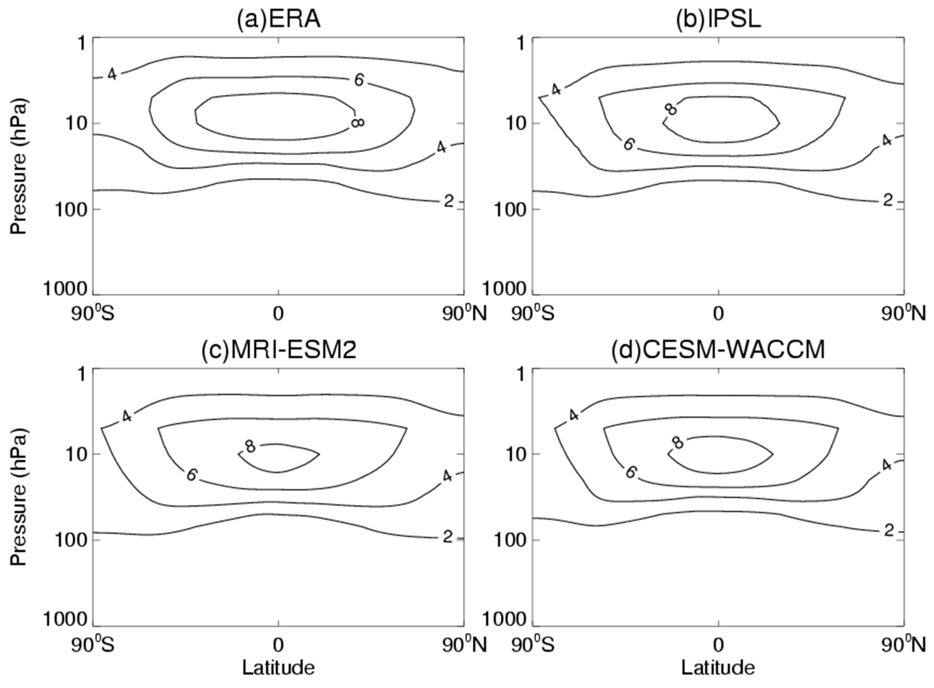
Figure 1 shows the distributions of climatological average ozone concentration extracted from the ERA-I reanalysis and simulated by three models. Compared with Figure 1a, all the three models (Figure 1b–d) can reproduce the climatological distribution of ozone in their historical simulation experiments under realistic forcing. Ozone concentration is high in the stratosphere, where the maximum concentration occurs at 10 hPa [1]. The meridional variation shows that ozone concentration is higher in the equatorial region and lower in the polar regions.
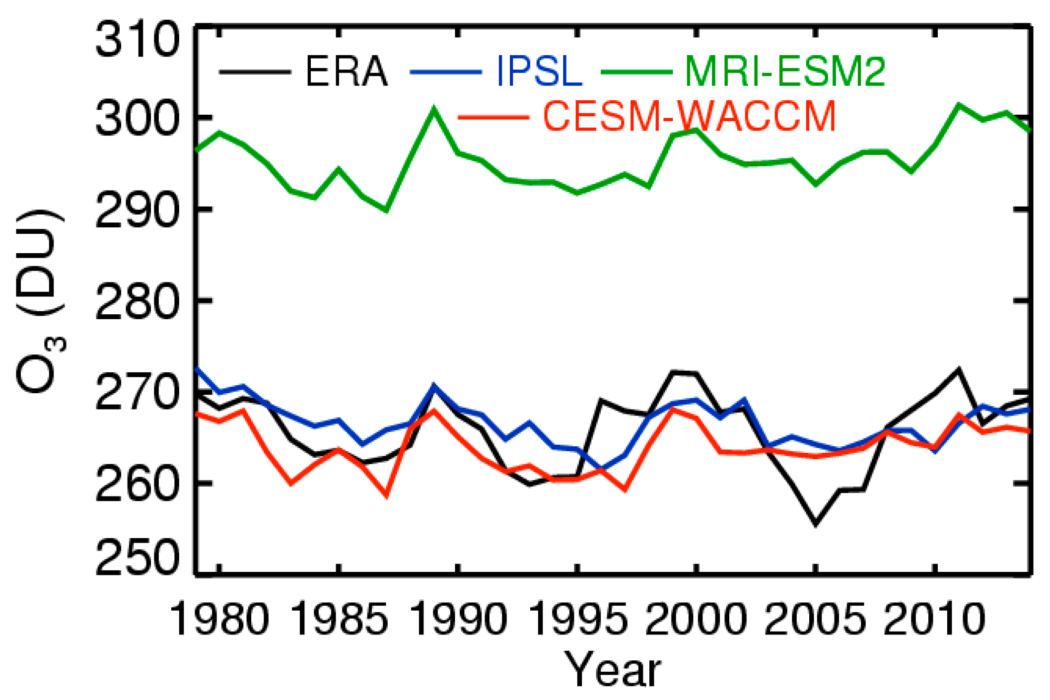
Total column ozone averaged over 30° S–30° N (Figure 2) shows that the correlation coefficients between the annual average total column ozone from the ERA-I and that simulated by the IPSL, the MRI-ESM2 and the CESM-WACCM models are 0.54, 0.61, and 0.59, respectively, which are significant at the 99% confidence level. This result indicates that the three models selected for the present study can realistically simulate the interannual variation of column ozone. As displayed in Figure 2, the climatological column ozone values simulated by the IPSL and the CESM-WACCM are 266.6 and 263.9DU, respectively, which are close to the value shown in the ERA-I reanalysis data (265.7 DU). The climatological column ozone value simulated by the MRI-ESM2 is 295.4 DU, which is much higher than that in the ERA-I. Generally, the historical simulation results indicate that climatological average total column ozone simulated by the IPSL and CESM-WACCM is close to that in the ERA-I in magnitude, whereas the MRI-ESM2 model can better simulate the interannual variation of the total column ozone.
3.2. Future Trend of Ozone Change
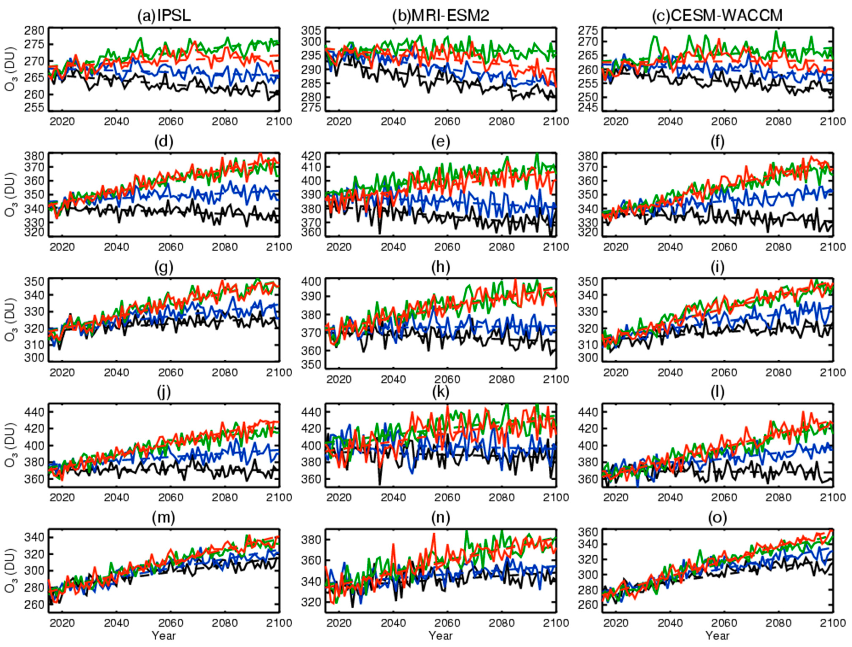
Figure 3 displays changes in total column ozone under various SSP scenarios at different latitudes. For the low latitudes (Figure 3a–c) the total column ozone would decrease under the SSP1-2.6 and SSP2-4.5 scenarios, and the decrease rate is the fastest under the SSP1-2.6 scenario with the largest value of 1.53 DU/decade simulated by the MRI-ESM2. Under the SSP-3.7 scenario, simulations of the IPSL and the CESM-WACCM indicate that the total column ozone would increase at the rates of 0.91 and 0.57 DU/decade, respectively. The decrease trend of the total column ozone is the slowest in the simulation of the MRI-ESM2 at the rates of 0.08 DU/decade. Under the SSP5-8.5 scenario, the IPSL and CESM-WACCM results indicate that the total column ozone would increase at the rates of 0.4 and 0.07 DU/decade, respectively, while result of the MRI-ESM2 indicates that the total column ozone would decrease at the rate of 0.88 DU/decade.
For the mid-latitudes of the Northern Hemisphere (Figure 3d–f) the total column ozone would decrease under the SSP1-2.6 scenario, and the decrease rate is the fastest with the largest value of 1.65 DU/decade simulated by the MRI-ESM2. Under the SSP2-4.5 scenario, the MRI-ESM2 result indicates that the total column ozone would decrease at the rate of 1.01 DU/decade, while results of the IPSL and CESM-WACCM indicate that the total column ozone would increase. The total column ozone would increase under the SSP3-7.0 and SSP5-8.5 scenarios. The changes of total column ozone is 3.95 DU/decade, 2.42 DU/decade and 4.71 DU/decade under the SSP5-8.5 scenario, respectively, which has the fastest increase rate among the four scenarios.
For the mid-latitudes of the Southern Hemisphere (Figure 3g–i) the total column ozone simulated by MRI-ESM2 model would decease at the rate of 0.55 DU/decade under the SSP1-2.6 scenario, and the other variation trends all increase in the future. The changes of total column ozone are 3.54 DU/decade (IPSL), 2.72 DU/decade (MRI-ESM2) and 4.12 DU/decade (CESM-WACCM) under SSP5-8.5 scenarios, respectively, which is the fastest increase rate among the four scenarios. Compared with the results in Northern Hemisphere (Figure 3d–f), the increase rate of IPSL and CESM-WACCM is larger and MRI-ESM2 is smaller under the SSP5-8.5 scenario.
The trends at the high-latitudes of the Northern Hemisphere (Figure 3j–l) are similar to that at the mid-latitudes of the Northern Hemisphere. The total column ozone would decrease under the SSP1-2.6 scenario, and the decrease rate is the fastest with the largest value of 0.81 DU/decade simulated by the MRI-ESM2. Under the SSP2-4.5 scenario, the MRI-ESM2 result indicates that the total column ozone would decrease at the rate of 0.71 DU/decade, while results of the IPSL and CESM-WACCM indicate that the total column ozone would increase. The total column ozone would increase under the SSP3-7.0 and SSP5-8.5 scenarios. The changes of total column ozone are 6.94 DU/decade (IPSL), 4.69 DU/decade (MRI-ESM2) and 7.93 DU/decade (CESM-WACCM) under the SSP5-8.5 scenario, respectively, which has the fastest increase rate among the four scenarios.
For the high-latitudes of the Southern Hemisphere (Figure 3m–o) the trends all increase under different scenarios. Under the SSP1-2.6 (SSP5-8.5) scenario, the total column ozone increase trend is the slowest at the rate of 1.61 DU/decade (4.94 DU/decade) simulated by the MRI-ESM2 and fastest at the rate of 5.59 DU/decade (9.97 DU/decade) simulated by the CESM-WACCM.
In the extratropic, the increase rate of the total column ozone simulated by the three models is the largest under the SSP5-8.5 scenario, and the increase rate is the smallest or the decrease rate is the largest under the SSP1-2.6 scenario. In this region, CESM-WACCM shows the largest increase rate and the MRI-ESM2 shows the largest decrease or smallest increase rate. In the low latitudes, IPSL shows the largest increase or smallest decrease rate, and the MRI-ESM2 shows the largest decrease rate.
The total column ozone at high-latitudes of the Southern Hemisphere simulated by the three models increases under all scenarios, i.e., the Antarctica ozone would gradually recover in the future.
However, the total column ozone at high-latitudes of the Northern Hemisphere simulated by the three models decreases under the SSP1-2.6 scenario, and it also decreases in the MRI-ESM2 model under the SSP2-4.5 scenario, which indicates that the Arctic ozone would never recover under the SSP1-2.6 scenario.
In the early spring of 1997 [43] and 2011 [44], an “ozone hole” appeared over the Arctic, and stratospheric ozone values over large parts of the Arctic in 2020 spring are lower than observed in any previous year [45,46,47,48,49]. All of the three ozone loss events related to extremely strong and cold polar vortices, when the temperature was low enough to form polar stratospheric clouds (PSCs), resulting in large stratospheric ozone losses [50]. Since the majority of the world’s population lives in the Northern Hemisphere, the research on Arctic ozone hole has great social significance. However, compared with the Antarctic ozone hole, ozone depletion in the Arctic has a much higher interannual variability because of higher dynamical activity in the Northern Hemisphere [44,51]. Austin and Wilson [52] pointed out that, despite interannual variability being greater in the future than in the past, the Arctic ozone would recover to the 1980 value in all recovery criterion. Bednarz et al. [53] also pointed out that, despite the large interannual dynamical variability being expected to continue in the future, resulting in reductions in springtime ozone columns, the recovery of Arctic ozone would continue in future. WMO [54] and Pommereau [55] pointed out that Arctic ozone loss will remain possible in cold winters in the future if the ozone depletion substance concentrations are above natural levels; this is because the increasing GHGs may cool the lower stratosphere and resulting in enhanced formation of PSCs in the Arctic. However, the result in Langematz et al. [56] indicates that no cooling would appear in March, which is the month when persistent low temperatures lead to large chemical ozone losses. Meanwhile in our result, the Arctic ozone would never recover under SSP1-2.6 scenario, and would gradually recover under other scenarios. There are some differences between our results and previous WMO assessment [54], which may be related to the scenario for the baseline estimate and some model updates. In addition to the Arctic ozone losses, Zhang et al. [57] found that the Arctic stratospheric polar vortex has been shifted toward Siberia during late winter over the period 1980–2015. Therefore, how the future Arctic ozone will change is far from conclusive and is worthy of further in-depth study.
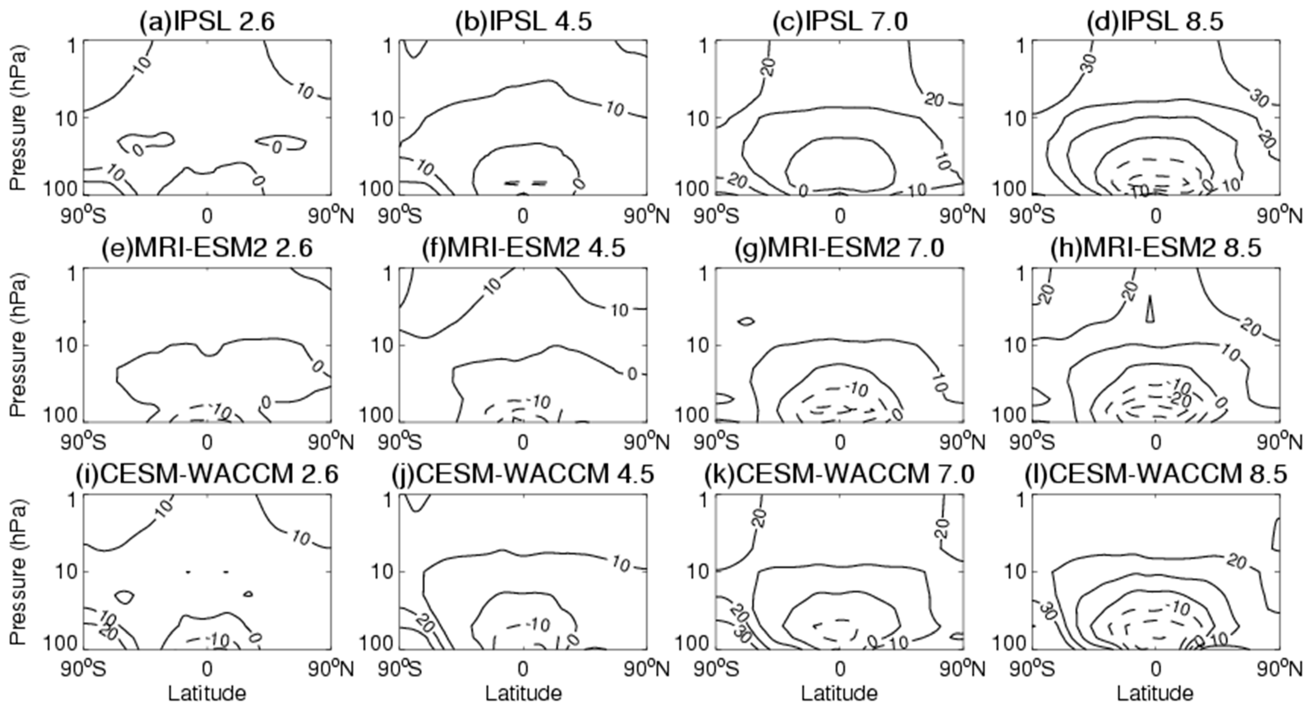
Figure 4 presents changes in stratospheric ozone concentration during 2091–2100 compared to that during 2015-2024 under different SSP scenarios. All the three models indicate that ozone would decrease in the lower tropical stratosphere, whereas it would increase outside the tropics and in the middle and upper tropical stratosphere. Under the four scenarios, the magnitude of ozone decrease in tropical middle and lower stratosphere would increase following the increase in social vulnerability and anthropogenic radiative forcing. Ozone in the middle and lower tropical stratosphere will decrease by 10% under the SSP1-2.6 scenario and by 30% under the SSP5-8.5 scenario, which is consistent with Eyring et al. [19] that in the topical lower stratosphere ozone decrease continuously from 1960 to 2100 due to projected increase in tropical upwelling because of the acceleration BD circulation. Outside the tropics and in tropical middle to upper stratosphere, the magnitude of ozone increase also would become lager as the social vulnerability and anthropogenic radiative forcing increase. Under the SSP1-2.6 scenario, ozone will increase by around 10% in upper levels in the extratropics; under the SSP8.5 scenario, the change can be up to 20% (MRI-ESM2 and CESM-WACCM) and 30% (IPSL).
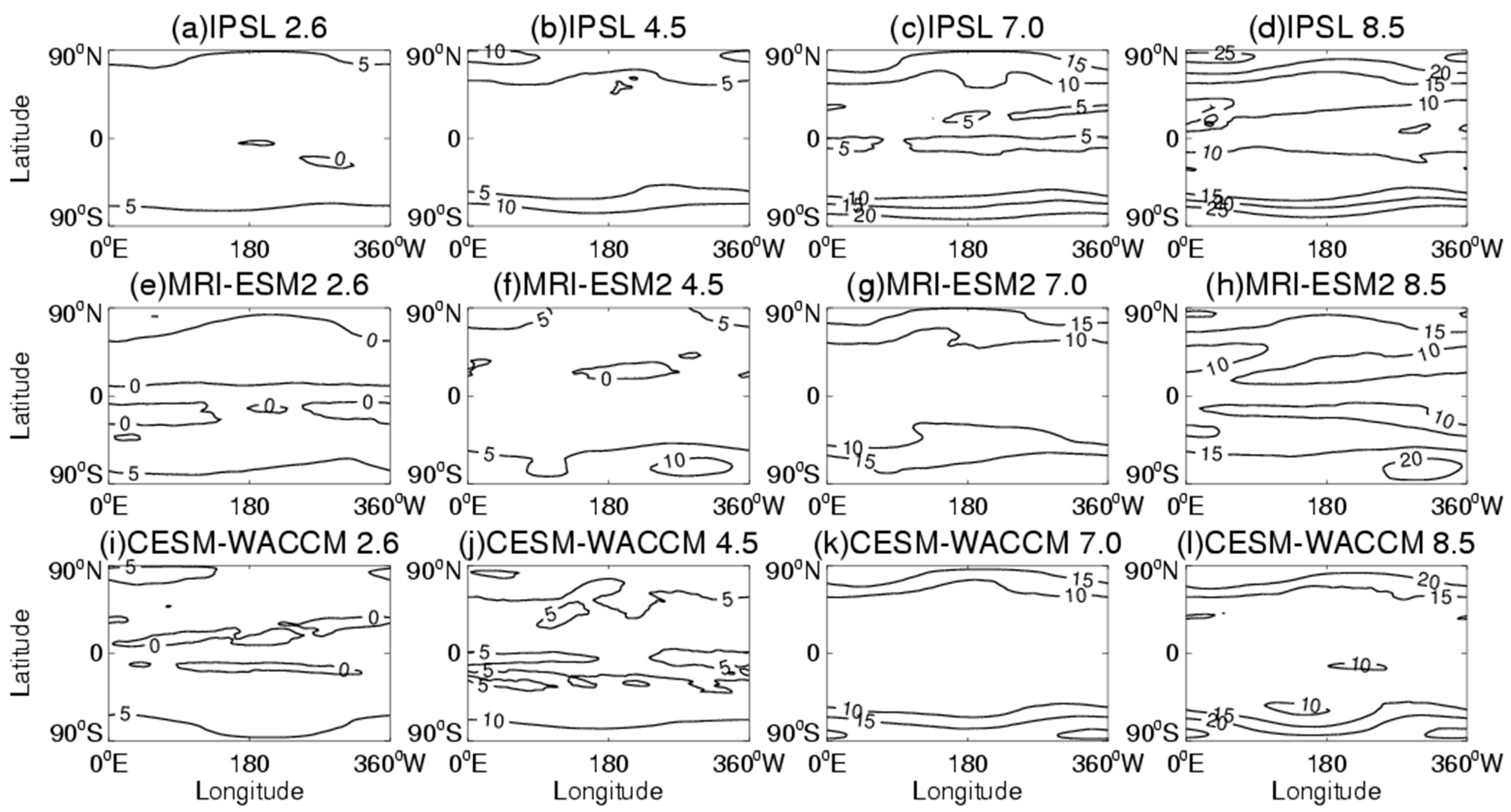
In order to better analyze ozone changes in different regions, Figure 5 displays ozone concentration changes at 10 hPa, which is the level where the maximum stratospheric ozone concentration occurs. Figure 5 shows that ozone concentration at 10 hPa will increase under all the four scenarios. Under the SSP1-2.6 scenario, ozone concentration at 10 hPa shows little change. Following the increase in social vulnerability and anthropogenic radiative forcing, the magnitude of ozone change in the middle stratosphere would increase, and the largest increase would occur in high-latitude regions. Under the SSP5-8.5 scenario, all three models indicate that ozone concentration will increase by 10% in the tropics and 15–20% in high-latitude regions.
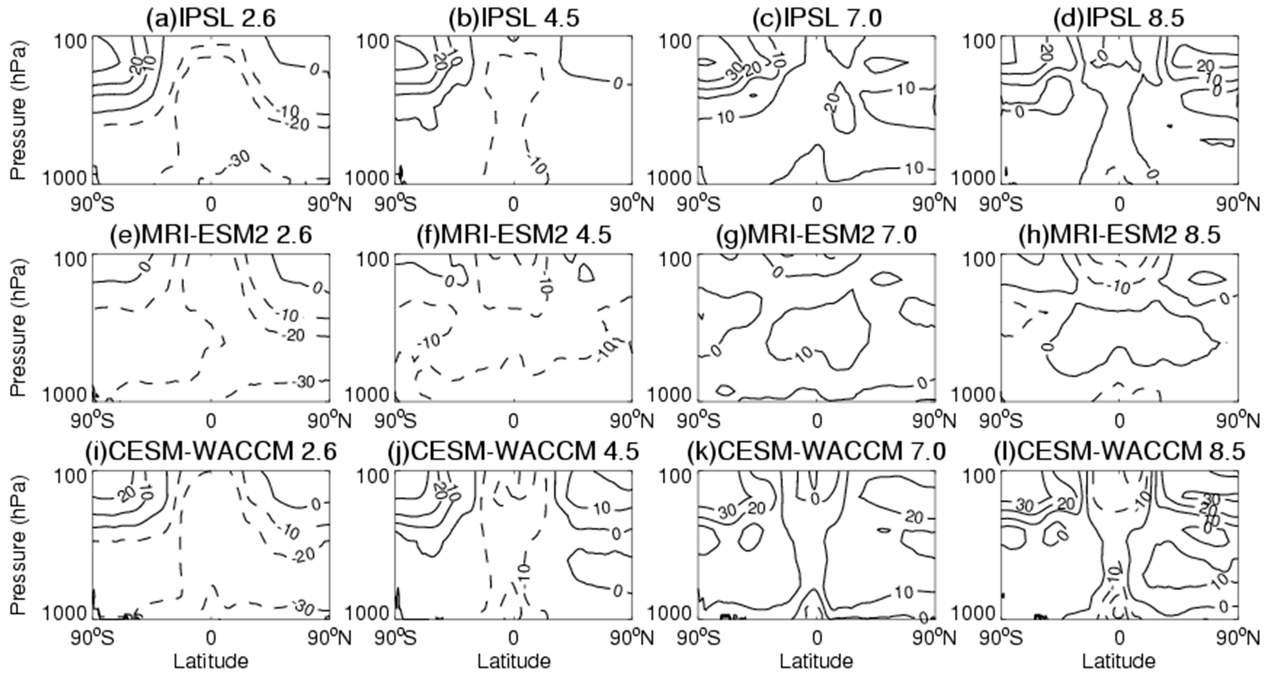
Figure 6 displays the three model simulations of tropospheric ozone concentration change during 2091–2100 compared to that during 2015–2024 under various SSP scenarios. Under the SSP1-2.6 scenario, tropospheric ozone concentration will decrease with the largest decrease of up to 30% occurring in the middle and lower tropical troposphere. Following the increase in social vulnerability and anthropogenic radiative forcing, tropospheric ozone concentration gradually increases. The results are consistent with previous research results as in a warming climate, tropospheric ozone loss can increase due to higher absolute humidity [58,59]. However, as the social vulnerability and anthropogenic radiative forcing is increasing there is a positive relationship between anthropogenic emissions and tropospheric ozone [60,61] as shown in Figure 6. Under the SSP2-4.5 scenario, the magnitude of decrease in tropical tropospheric ozone concentration is about 10%. The CESM-WACCM result indicates that ozone concentration obviously increases in mid and high-latitude regions. Under the SSP3-7.0 scenario, tropospheric ozone concentration overall will increase. Under the SSP5-8.5 scenario, the IPSL result indicates that tropical lower tropospheric ozone concentration will decrease; while results of the MRI-ESM and CESM-WACCM show that ozone concentration will decrease in the upper and lower levels of tropical troposphere.
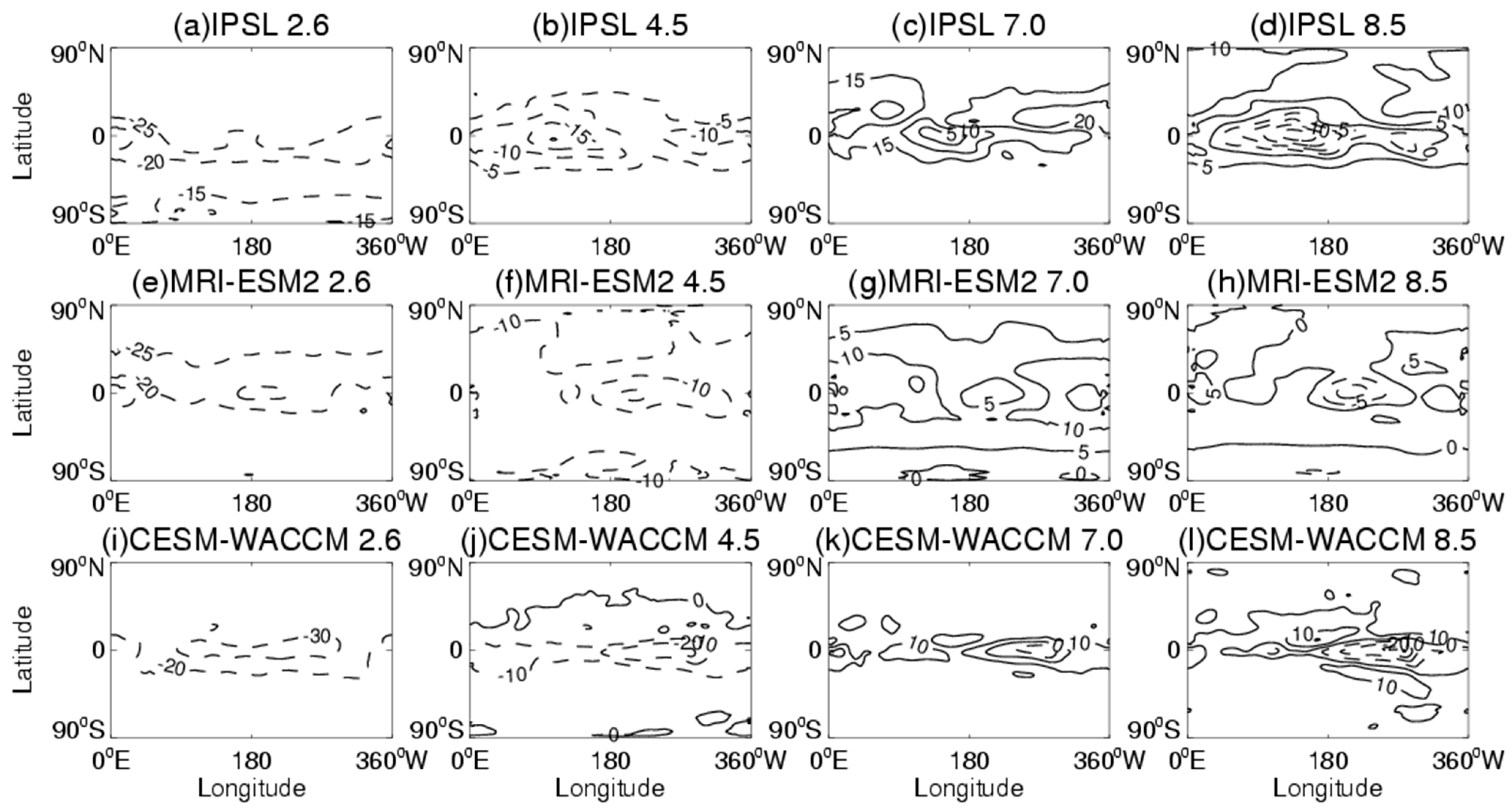
Spatial pattern of ozone concentration change in the middle troposphere is further analyzed (Figure 7). Under the SSP1-2.6 and SSP2-4.5 scenarios, ozone concentration will decrease with the largest decrease occurring in the equatorial region. Under the SSP7.0 scenario, 500 hPa ozone concentration will increase. Under the SSP5-8.5 scenario, 500 hPa ozone concentration will increase outside the tropics and decrease in some areas of the tropics. The IPSL result shows large ozone concentration decrease in the tropical regions of the Eastern Hemisphere, while results of the MRI-ESM2 and CESM-WACCM indicate that the largest decrease will occur in the tropical regions of the Western Hemisphere. Overall, following the increase in social vulnerability and anthropogenic radiative forcing, 500 hPa ozone concentration will increase.
3.3. Variation Trend of Ozone in Tropic
Stratospheric ozone absorbs ultraviolet (UV) radiation and protects life on earth from harmful UV radiation. Therefore, it is very important to study the trend of stratospheric ozone change. Figure 1 shows that the ozone concentration is largest at the low latitudes, so the ozone variation trends at low latitudes are analysed next.
Table 1 lists changes in tropical total column ozone. Table 2 and Table 3 list changes in tropical stratospheric and tropospheric total column ozone, respectively. The IPSL and CESM-WACCM results indicate increase trends in tropical stratospheric column ozone, while the MRI-ESM2 shows a decrease trend, although the results of the CESM-WACCM suggest that stratospheric column ozone will slightly increase under the SSP5-8.5 scenario. In all three models, there are decrease trends under the SSP1-2.6 and SSP2-4.5 scenarios in tropical tropospheric column ozone, and an increase trend under the SSP3-7.0 scenario. Under the SSP5-8.5 scenario, the MRI-ESM2 and CESM-WACCM results indicate decrease trends, while the IPSL result indicates slightly increase trend. That is, although total tropical column ozone shows a decrease trend under the SSP1-2.6 and SSP2-4.5 scenarios (Figure 3) and an increase trend can also be found in some model simulations under the SSP3-7.0 and SSP5-8.5 scenarios, relatively large differences can be found in stratospheric ozone change between the three model results. Nevertheless, certain regularities of changes in stratospheric and tropospheric ozone can still be found in these results.
Table 2 shows that with the increases in social vulnerability and anthropogenic radiative forcing, the change of the stratospheric column ozone in tropical regions is not linear. Compared with the SSP2-4.5 and SSP5-8.5 scenarios, the SSP1-2.6 and SSP3-7.0 scenarios are more conducive to the increase in total stratospheric ozone. Comparing the results under the SSP1-2.6 and SSP2-4.5 scenarios shown in Figure 4 and Figure 5, it is found that the increase in stratospheric ozone is not obvious, while the decrease in tropospheric ozone can reach up to 30%. Comparing with the results under the SSP1-2.6 and SSP2-4.5 scenarios shown in Table 2 and Table 3, it can be found that the decrease trend of the total column ozone in the tropical area under the SSP1-2.6 and SSP2-4.5 scenarios shown in Figure 3 is largely attributed to the decrease in tropical tropospheric ozone. Taking the IPSL model simulation under the SSP2.6 scenario as an example, the trend of the total column ozone in the tropics is −0.64 DU/decade, of which the trend of the tropospheric ozone column is −0.92 DU/decade and the trend of the stratospheric column ozone is 0.28 DU/decade. In other words, the ozone concentration in the stratosphere is increasing, yet the decrease in the total ozone column in the tropical troposphere has led to a decreasing trend in the total ozone column in the entire tropical region. In these three models, the trend of the stratospheric column ozone in the tropics is almost the same under the SSP1-2.6 and SSP3-7.0 scenarios. However, the tropospheric total column ozone under the SSP1-2.6 scenario has a decreasing trend, whereas it has an increasing trend under the SSP3-7.0 scenario. As a result, the decreasing trend of the total column ozone is the fastest under the SSP1-2.6 scenario (Figure 3) and the slowest under the SSP3-7.0 scenario, or the total column ozone may even increase under the SSP3-7.0 scenario.
Tropospheric ozone decreases under the SSP1-2.6 and SSP2-4.5 scenarios. In contrast, under the SSP3-7.0 scenario, the tropospheric ozone concentration increases significantly, with an increase rate of up to 10%. Under the SSP5-8.5 scenario, although the ozone concentration decreases in the middle and lower troposphere in tropics, it increases in the middle and lower troposphere outside the tropics. Tropospheric ozone is a pollutant that is harmful to organisms and is one of the components of photochemical smog. The increase in tropospheric ozone concentration will have adverse effects on life on Earth.
4. Conclusions
In CMIP6, the participating models have been further developed and new emission scenarios, so-called SSPs, have been established. This study compares and analyzes simulations of ozone under different scenarios by three CMIP6 models (IPSL-CM6A, MRI-ESM2 and CESM-WACCM). It is found that in the extratropic, CESM-WACCM shows the largest increase rate and the MRI-ESM2 shows the largest decrease or smallest increase rate of the total column ozone. In the tropics, IPSL shows the largest increase or smallest decrease rate, and the MRI-ESM2 shows the largest decrease rate.
Results indicate that, as the social vulnerability and anthropogenic radiative forcing is increasing, the change of total column ozone in the tropical stratosphere is not linear. Compared to the SSP2-4.5 and SSP5-8.5 scenarios, the SSP1-2.6 and SSP3-7.0 are more favorable for the increase in stratospheric ozone mass in the tropics. The total column ozone at the mid to high latitudes shows decrease trends under SSP1-2.6 scenario, which indicates that the Arctic ozone would never recover under SSP1-2.6 scenario. In addition, under SSP2-4.5 scenario, the MRI-ESM2 model result also shows a decrease trend. However the total column ozone at high-latitudes of the Southern Hemisphere simulated by the three models increase under all scenarios, i.e., the Antarctica ozone would gradually recover in all scenarios.
Under the SSP1-2.6 and SSP2-4.5 scenarios, the trend of tropical total column ozone is mainly determined by the trend of column ozone in the tropical troposphere. Under the SSP3-7.0 scenario, tropospheric ozone concentration will significantly increase; under the SSP5-8.5 scenario, ozone concentration will distinctly increase in the middle and lower troposphere. High social vulnerability and relatively strong anthropogenic radiative forcing will lead to increases in tropospheric ozone concentration, which will have adverse impacts on life on Earth.
Author Contributions
Conceptualization, L.S. and J.L.; data curation, C.W.; writing-original draft preparation, L.S.; writing-review and editing, J.L. All authors have read and agreed to the published version of the manuscript.
Funding
This research was funded by the National Natural Science Foundation of China (41705025, 42075060).
Institutional Review Board Statement
Not applicable.
Informed Consent Statement
Not applicable.
Data Availability Statement
The data sets used here are publicly available. The ERA-I data is from the European Centre for Medium-Range Weather Forecasts (ECMWF) at https://apps.ecmwf.int/datasets/. The CMIP6 data is from the World Climate Research Programme (WCRP) at https://esgf-node.llnl.gov/projects/cmip6/.
Acknowledgments
We acknowledge the ozone dataset provided by ECMWF and WCRP.
Conflicts of Interest
The authors declare no conflict of interest. The funders had no role in the design of the study; in the collection, analyses, or interpretation of data; in the writing of the manuscript, or in the decision to publish the results.
References
- Andrews, D.G.; Holton, J.R.; Leovy, C.B. Middle Atmosphere Dynamics; Academic Press: San Diego, CA, USA; New York, NY, USA; Boston, FL, USA; London, UK; Sydney, New South Wales, Australia; Tokyo, Japan; Toronto, ON, Canada, 1987. [Google Scholar]
- Wofsy, S.C.; Elroy, M.B.; Yung, Y.L. The chemistry of atmospheric bromine. Geophys. Res. Lett. 1975, 2, 215–218. [Google Scholar] [CrossRef] [Green Version]
- Yung, Y.L.; Pinto, J.P.; Watson, R.T. Atmospheric Bromine and Ozone Perturbations in the Lower Stratosphere. J. Atmos. Sci. 1980, 37, 339–353. [Google Scholar] [CrossRef] [Green Version]
- Prather, M.J.; Mcelroy, M.B.; Wofsy, S.C. Reductions in ozone at high concentrations of stratospheric halogens. Nature 1984, 312, 227–231. [Google Scholar] [CrossRef] [PubMed]
- Randel, W.J.; Wu, F. A stratospheric ozone profile data set for 1979–2005: Variability, trends, and comparisons with column ozone data. J. Geophys. Res. Atmos. 2007, 112. [Google Scholar] [CrossRef] [Green Version]
- Montzka, S.A.; Butler, J.H.; Myers, R.C.; Thompson, T.M.; Swanson, T.H.; Clarke, A.D.; Lock, L.T.; Elkins, J.W. Decline in the tropospheric abundance of halogen from halocarbons: Implications for stratospheric. Science 1996, 272, 1318–1322. [Google Scholar] [CrossRef] [PubMed]
- Anderson, J.; Russell, J.M.; Solomon, S. Halogen Occultation Experiment confirmation of stratospheric chlorine decreases in accordance with the Montreal Protocol. J. Geophys. Res. Atmos. 2000, 105, 4483–4490. [Google Scholar] [CrossRef]
- Newchurch, M.J. Evidence for slowdown in stratospheric ozone loss: First stage of ozone recovery. J. Geophys. Res. Atmos. 2003, 108, D16. [Google Scholar] [CrossRef] [Green Version]
- Randeniya, L.K.; Vohralik, P.F.; Plumb, I.C. Stratospheric ozone depletion at northern mid latitudes in the 21st century: The importance of future concentrations of greenhouse gases nitrous oxide and methane. Geophys. Res. Lett. 2002, 29, 101–104. [Google Scholar] [CrossRef]
- Rosenfield, J.E.; Douglass, A.R.; Considine, D.B. The impact of increasing carbon dioxide on ozone recovery. J. Geophys. Res. Atmos. 2002, 107, 7–9. [Google Scholar] [CrossRef]
- Brewer, A.W. Evidence for a world circulation provided by the measurements of helium and water vapour distribution in the stratosphere. Q. J. R. Meteorol. Soc. 1949, 75, 351–363. [Google Scholar] [CrossRef]
- Dobson, G.M.B. Origin and Distribution of the Polyatomic Molecules in the Atmosphere. Proc. R. Soc. Lond. 1956, 236, 187–193. [Google Scholar]
- Rind, D.; Suozzo, R.; Balachandran, N. Climate Change and the Middle Atmosphere. Part I: The Doubled CO2 Climate. J. Clim. 1990, 11, 475–494. [Google Scholar] [CrossRef] [Green Version]
- Rind, D.; Lerner, J.; Mclinden, C. Changes of tracer distributions in the doubled CO2 climate. J. Geophys. Res. Atmos. 2001, 106, 28061–28079. [Google Scholar] [CrossRef] [Green Version]
- Garcia, R.R.; Randel, W.J. Acceleration of the Brewer-Dobson Circulation due to Increases in Greenhouse Gases. J. Atmos. Sci. 2008, 65, 2731–2739. [Google Scholar] [CrossRef]
- McLandress, C.; Jonsson, A.I.; Plummer, D.A.; Reader, M.C.; Scinocca, J.F.; Shepherd, T.G. Separating the Dynamical Effects of Climate Change and Ozone Depletion. Part I: Southern Hemisphere Stratosphere. J. Clim. 2010, 23, 5002–5020. [Google Scholar] [CrossRef] [Green Version]
- Polvani, L.M.; Wang, L.; Aquila, V.; Waugh, D.W. The Impact of Ozone Depleting Substances on Tropical Upwelling, as Revealed by the Absence of Lower Stratospheric Cooling since the Late 1990s. J. Clim. 2016, 30, 2523–2534. [Google Scholar] [CrossRef] [Green Version]
- Polvani, L.M.; Abalos, M.; Garcia, R.; Kinnison, D.; Randel, W.J. Significant Weakening of Brewer-Dobson Circulation Trends over the 21st Century as a Consequence of the Montreal Protocol. Geophys. Res. Lett. 2017, 45, 401–409. [Google Scholar] [CrossRef] [Green Version]
- Eyring, V.; Cionni, I.; Bodeker, G.E.; Charlton-Perez, A.J.; Kinnison, D.E.; Scinocca, J.F.; Waugh, D.W.; Akiyoshi, H.; Bekki, S.; Chipperfield, M.P.; et al. Multi-model assessment of stratospheric ozone return dates and ozone recovery in CCMVal-2 models. Atmos. Chem. Phys. 2010, 10, 9451–9472. [Google Scholar] [CrossRef] [Green Version]
- Chipperfield, M.P.; Feng, W. Comment on: Stratospheric Ozone Depletion at northern mid-latitudes in the 21st century: The importance of future concentrations of greenhouse gases nitrous oxide and methane. Geophys. Res. Lett. 2003, 30, 7. [Google Scholar] [CrossRef] [Green Version]
- Ravishankara, A.R.; Daniel, J.S.; Portmann, R.W. Nitrous Oxide (N2O): The dominant ozone-depleting substance emitted in the 21st century. Science 2009, 326, 123–125. [Google Scholar] [CrossRef] [PubMed] [Green Version]
- Morgenstern, O.; Zeng, G.; Abraham, N.L.; Telford, P.J.; Braesicke, P.; Pyle, J.A.; Hardiman, S.C.; O’Connor, F.M.; Johnson, C.E. Correction to “Impacts of climate change, ozone recovery, and increasing methane on surface ozone and the tropospheric oxidizing capacity”. J. Geophys. Res. Atmos. 2014, 118, 1028–1041. [Google Scholar] [CrossRef]
- Kirner, O.; Ruhnke, R.; Sinnhuber, B.M. Chemistry-Climate Interactions of Stratospheric and Mesospheric Ozone in EMAC Long-Term Simulations with Different Boundary Conditions for CO2, CH4, N2O, and ODS. Atmos. Ocean 2015, 53, 140–152. [Google Scholar] [CrossRef]
- Egorova, T.A.; Rozanov, E.; Arsenovic, P.; Sukhodolov, T. Ozone Layer Evolution in the Early 20th Century. Atmosphere 2020, 11, 169. [Google Scholar] [CrossRef] [Green Version]
- Zubov, V.; Rozanov, E.; Egorova, T.; Karol, I.; Schmutz, W. Role of external factors in the evolution of the ozone layer and stratospheric circulation in 21st century. Atmos. Chem. Phys. Discuss. 2012, 13, 4697–4706. [Google Scholar] [CrossRef] [Green Version]
- Eyring, V.; Waugh, D.W.; Bodeker, G.E.; Cordero, E.; Akiyoshi, H.; Austin, J.; Beagley, S.R.; Boville, B.A.; Braesicke, P.; Brühl, C.; et al. Multimodel projections of stratospheric ozone in the 21st century. J. Geophys. Res. Atmos. 2007, 112, D16303. [Google Scholar] [CrossRef]
- Eyring, V.; Arblaster, J.M.; Cionni, I.; Sedlacek, J.; Perlwitz, J.; Young, P.J.; Bekki, S.; Bergmann, D.; Cameron-Smith, P.; Collins, W.J.; et al. Long-term ozone changes and associated climate impacts in CMIP5 simulations. J. Geophys. Res. Atmos. 2013, 118, 5029–5060. [Google Scholar] [CrossRef] [Green Version]
- Dhomse, S.S.; Kinnison, D.; Chipperfield, M.P.; Salawitch, R.J.; Cionni, I.; Hegglin, M.I.; Abraham, N.L.; Akiyoshi, H.; Archibald, A.T.; Bednarz, E.M.; et al. Estimates of Ozone Return Dates from Chemistry-Climate Model Initiative Simulations. Atmos. Chem. Phys. 2018, 18, 8409–8438. [Google Scholar] [CrossRef] [Green Version]
- Langematz, U. Future ozone in a changing climate. Comptes Rendus Geosci. 2018, 350, 403–409. [Google Scholar] [CrossRef]
- Eyring, V.; Bony, S.; Meehl, G.A.; Senior, C.A.; Stevens, B.; Stouffer, R.J.; Taylor, K.E. Overview of the Coupled Model Intercomparison Project Phase 6 (CMIP6) experimental design and organization. Geoentific Model Dev. 2016, 9, 1937–1958. [Google Scholar] [CrossRef] [Green Version]
- Neill, B.C.; Kriegler, E.; Riahi, K.; Ebi, K.L.; Hallegatte, S.; Carter, T.R.; Mathur, R.; Vuuren, D.P. A new scenario framework for climate change research: The concept of shared socioeconomic pathways. Clim. Chang. 2014, 122, 387–400. [Google Scholar]
- Neill, B.C.; Tebaldi, C.; Vuuren, D.P.; Eyring, V.; Friedlingstein, P.; Hurtt, G.; Knutti, R.; Kriegler, E.; Lamarque, J.F.; Lowe, J.; et al. The Scenario Model Intercomparison Project (ScenarioMIP) for CMIP6. Geosci. Model Dev. 2016, 9, 3461–3482. [Google Scholar] [CrossRef] [Green Version]
- Neill, B.C.; Kriegler, E.; Ebi, K.L.; Benedict, E.K.; Riahi, K.; Rothman, D.S.; Ruijven, B.J.; Vuuren, D.P.; Birkmann, J.; Kok, K.; et al. The roads ahead: Narratives for shared socioeconomic pathways describing world futures in the 21st century. Glob. Environ. Chang. 2017, 42, 169–180. [Google Scholar]
- Riahi, K.; Vuuren, D.P.; Kriegler, E.; Edmonds, J.; O’Neill, B.C.; Fujimori, S.; Bauer, N.; Calvin, K.; Dellink, R.; Fricko, O.; et al. The Shared Socioeconomic Pathways and their energy, land use, and greenhouse gas emissions implications: An overview. Glob. Environ. Chang. 2017, 42, 153–168. [Google Scholar] [CrossRef] [Green Version]
- Berrisford, P.; Dee, D.P.; Poli, P.; Brugge, R.; Fielding, M.; Fuentes, M.; Kallberg, P.W.; Kobayashi, S.; Uppala, S.; Simmons, A. The ERA. ERA Rep. Ser. 2011, 2, 1–23. [Google Scholar]
- Boucher, O.; Servonnat, J.; Albright, A.L.; Aumont, O.; Balkanski, Y.; Bastrikov, V.; Bekki, S.; Bonnet, R.; Bony, S.; Bopp, L.; et al. Presentation and evaluation of the IPSL-CM6A-LR climate model. J. Adv. Modeling Earth Syst. 2020, 12, e2019MS002010. [Google Scholar] [CrossRef]
- Hourdin, F.; Rio, C.; Jam, A.; Traore, A.K.; Musta, I. Convective Boundary Layer Control of the Sea Surface Temperature in the Tropics. J. Adv. Modeling Earth Syst. 2020, 12, e2019MS001988. [Google Scholar] [CrossRef] [Green Version]
- Madec, G.; the NEMO System Team. NEMO Ocean Engine, Version 3.6 Stable. 2016. Available online: https://www.nemo-ocean.eu/doc/ (accessed on 20 January 2020).
- Krinner, G.; Viovy, N.; Noblet, D.N.; Ogée, J.; Polcher, J.; Friedlingstein, P.; Ciais, P.; Sitch, S.; Prentice, I.C. A dynamic global vegetation model for studies of the coupled atmosphere-biosphere system. Glob. Biogeochem. Cycles 2005, 19, GB1015. [Google Scholar] [CrossRef]
- Yukimoto, S.; Koshiro, T.; Kawai, H.; Oshima, N.; Yoshida, K.; Urakawa, S.; Tsujino, H.; Deushi, M.; Tanaka, T.; Hosaka, M.; et al. MRI MRI-ESM2.0 Model Output Prepared for CMIP6 CMIP. Version 20200120. Earth System Grid Federation. 2019. Available online: https://0-doi-org.brum.beds.ac.uk/10.22033/ESGF/CMIP6.621 (accessed on 20 January 2020).
- Gettelman, A.; Hannay, C.; Bacmeister, J.T.; Neale, R.B.; Pendergrass, A.G.; Danabasoglu, G.; Lamarque, J.F.; Fasullo, J.T.; Bailey, D.A.; Lawrence, D.M.; et al. High Climate Sensitivity in the Community Earth System Model Version 2 (CESM2). Geophys. Res. Lett. 2019, 46, 8329–8337. [Google Scholar] [CrossRef]
- Knutti, R.; Masson, D.; Gettelman, A. Climate model genealogy: Generation CMIP5 and how we got there. Geophys. Res. Lett. 2013, 40, 1194–1199. [Google Scholar] [CrossRef]
- Newman, P.A.; Gleason, J.F.; Mcpeters, R.D.; Stolarski, R.S. Anomalously low ozone over the Arctic. Geophys. Res. Lett. 1997, 24, 2689–2692. [Google Scholar] [CrossRef]
- Manney, G.L.; Santee, M.L.; Rex, M.; Livesey, M.J.; Pitts, M.C.; Veefkind, P.; Nash, E.R.; Wohltmann, I.; Lehmann, R.; Froidevaux, L.; et al. Unprecedented Arctic ozone loss in 2011. Nature 2011, 478, 469–475. [Google Scholar] [CrossRef] [PubMed]
- Dameris, M.; Loaola, D.; Nutzel, M.; Egbers, M.C.; Lerot, C.; Romahn, F.; Roozendael, M. First description and classification of the ozone hole over the Arctic in boreal spring 2020. Atmos. Chem. Phys. Discuss. 2020, 1–26. [Google Scholar] [CrossRef]
- Inness, A.; Chabrillat, S.; Flemming, J.; Huijnen, V.; Langenrock, B.; Nicolas, J.; Polichtchouk, I.; Razinger, M. Exceptionally low Arctic stratospheric ozone in spring 2020 as seen in the CAMS reanalysis. J. Geophys. Res. Atmos. 2020, 125, e2020JD033563. [Google Scholar] [CrossRef]
- Lawrence, Z.D.; Perlwitz, J.; Butler, A.H.; Manney, G.L.; Newman, P.A.; Lee, S.H.; Nash, E.R. The Remarkably Strong Arctic Stratospheric Polar Vortex of Winter 2020: Links to Record-Breaking Arctic Oscillation and Ozone Loss. J. Geophys. Res. Atmos. 2020, 125, e2020JD033271. [Google Scholar] [CrossRef]
- Rao, J.; Garfinkel, C.I. Arctic Ozone Loss in March 2020 and Its Seasonal Prediction in CFSv2: A Comparative Study with the 1997 and 2011 Cases. J. Geophys. Res. Atmos. 2020, 125, e2020JD033524. [Google Scholar] [CrossRef]
- Wohltmann, I.; Gathen, P.; Lehmann, R.; Maturilli, M.; Deckelmann, H.; Manney, G.L.; Davies, J.; Tarasick, D.; Jepsen, N.; Kivi, R.; et al. Near complete local reduction of Arctic stratospheric ozone by severe chemical loss in spring 2020. Geoph. Res. Lett. 2020, 47, e2020GL089547. [Google Scholar] [CrossRef]
- Manney, G.L.; Livesey, N.J.; Santee, M.L.; Froidevaux, L.; Lambert, A.; Lawrence, Z.; Millan, L.; Neu, J.L.; Read, W.G.; Schwartz, M.J.; et al. Record-Low Arctic Stratospheric Ozone in 2020: MLS Observations of Chemical Processes and Comparisons with Previous Extreme Winters. Geophys. Res. Lett. 2020, 47, e2020GL089063. [Google Scholar] [CrossRef]
- Solomon, S.; Haskins, J.; Ivy, D.J.; Min, F. Fundamental differences between Arctic and Antarctic ozone depletion. Proc. Natl. Acad. Sci. USA 2014, 111, 6220–6225. [Google Scholar] [CrossRef] [Green Version]
- Austin, J.; Wilson, R.J. Ensemble simulations of the decline and recovery of stratospheric ozone. J. Geophys. Res. Atmos. 2006, 111, D08301. [Google Scholar] [CrossRef] [Green Version]
- Bednarz, E.M.; Maycock, A.C.; Abraham, N.L.; Braesicke, P.; Dessens, O.; Pyle, J.A. Future Arctic ozone recovery: The importance of chemistry and dynamics. Atmos. Chem. Phys. 2016, 16, 12159–12176. [Google Scholar] [CrossRef] [Green Version]
- WMO (World Meteorological Organization). Scientific Assessment of Ozone Depletion: 2018; Global Ozone Research and Monitoring Project-Report: Geneva, Swizerland, 2018; Volume 58, p. 588. [Google Scholar]
- Pommereau, J.P.; Goutail, F.; Pazmino, A.; Lefevre, F.; Chipperfield, M.P.; Feng, W.H.; Roozendael, M.V.; Jepsen, N.; Hansen, G.; Kivi, R.; et al. Recent Arctic ozone depletion: Is there an impact of climate change? Comptes Rendus Geosci. 2018, 350, 347–353. [Google Scholar] [CrossRef]
- Langematz, U.; Meul, S.; Grunow, K.; Romanowsky, E.; Oberlander, S.; Abalichin, J.; Kubin, A. Future Arctic temperature and ozone: The role of stratospheric composition changes. J. Geophys. Res. Atmos. 2014, 119, 2092–2112. [Google Scholar] [CrossRef]
- Zhang, J.; Tian, W.; Xie, F.; Pyle, J.A.; Keeble, J.; Wang, T. The influence of zonally asymmetric stratospheric ozone changes on the Arctic polar vortex shift. J. Clim. 2020, 33, 4641–4658. [Google Scholar] [CrossRef] [Green Version]
- Johnson, C.E.; Collins, W.J.; Stevenson, D.S.; Derwent, R.G. Relative roles of climate and emissions changes on future tropospheric oxidant concentrations. J. Geophys. Res. Atmos. 1999, 104, 18631–18645. [Google Scholar] [CrossRef] [Green Version]
- Zeng, G.; Pyle, J.A.; Young, P.J. Impact of climate change on tropospheric ozone and its global budgets[J]. Atmos. Chem. Phys. Discuss. 2008, 8, 369–387. [Google Scholar] [CrossRef] [Green Version]
- Stevenson, D.S.; Dentener, F.J.; Schultz, M.G.; Ellingsen, K.; Noije, T.P.; Wild, O.; Zeng, G.; Amann, M.; Atherton, C.S.; Bell, N.; et al. Multimodel ensemble simulations of present-day and near-future tropospheric ozone. J. Geophys. Res. 2006, 111, D08301. [Google Scholar] [CrossRef] [Green Version]
- Young, P.L.; Archibald, A.T.; Bowman, K.W.; Lamarque, J.F.; Naik, V.; Stevenson, D.S.; Tilmes, S.; Voulgarakis, A.; Wild, O.; Bergmann, D. Pre-industrial to end 21st century projections of tropospheric ozone from the Atmospheric Chemistry and Climate Model Intercomparison Project (ACCMIP). Atmos. Chem. Phys. 2013, 13, 2063–2090. [Google Scholar] [CrossRef] [Green Version]
Figure 1.
Height-latitude distributions of climatological ozone concentration extracted from the ERA-I and simulated by the three models for the period of 1979–2014 (unit: 10-6mol/mol). (a) ERA (b) IPSL (c) MRI-ESM2 (d) CESM-WACCM
Figure 1.
Height-latitude distributions of climatological ozone concentration extracted from the ERA-I and simulated by the three models for the period of 1979–2014 (unit: 10-6mol/mol). (a) ERA (b) IPSL (c) MRI-ESM2 (d) CESM-WACCM

Figure 2.
Total column ozone for the period of 1979–2014 averaged over 30° S–30° N for the ERA-I reanalysis and model simulations (units: DU).
Figure 2.
Total column ozone for the period of 1979–2014 averaged over 30° S–30° N for the ERA-I reanalysis and model simulations (units: DU).

Figure 3.
Trends of total column ozone change under different SSP scenarios. The first, second and thrid column is the result of IPSL (a,d,g,j,m), MRI-ESM2 (b,e,h,k,n) and CESM-WACCM (c,f,i,l,o) model, respectively. The first (a–c), second (d–f), third (g–i), fourth (j–l) and fifth (m–o) row is the trends of total column ozone change between 30° S and 30° N, 30° N and 60° N, 30° S and 60° S, 60° N and 90° N, and 60° S and 90° S for the period from 2015 to 2100, respectively. Black, blue, green and red lines represent the SSP1-2.6, SSP2-4.5, SSP3-7.0 and SSP5-8.5 scenarios, respectively. Solid lines represent the simulated values, and dashed lines are trend lines (unit: DU).

Figure 4.
Height-latitude cross sections of stratospheric ozone concentration change during 2091–2100 compared to that during 2015–2024 under different SSP scenarios (unit: percentage). The first, second and third row is the result of IPSL (a–d), MRI-ESM2 (e–h) and CESM-WACCM (i–l) model, respectively. The first, second, third and forth column is the result under the SSP 1-2.6 (a,e,i), 2-4.5 (b,f,j), 3-7.0 (c,g,k) and 5-8.5 (d,h,l) scenario, respectively. The positive and negative contours are represented by solid and dashed line.

Figure 5.
Changes in ozone concentration at 10 hPa during 2091–2100 compared to that during 2015–2024 under different SSP scenarios (unit: percentage). The first, second and third row is the result of IPSL (a–d), MRI-ESM2 (e–h) and CESM-WACCM (i–l) model, respectively. The first, second, third and forth column is the result under the SSP1-2.6 (a,e,i), 2-4.5 (b,f,j), 3-7.0 (c,g,k) and 5-8.5 (d,h,l) scenario, respectively.

Figure 6.
Height–latitude cross sections of tropospheric ozone concentration change during 2091–2100 compared to that during 2015–2024 under various SSP scenarios (unit: percentage). The first, second and third row is the result of IPSL (a–d), MRI-ESM2 (e–h) and CESM-WACCM (i–l) model, respectively. The first, second, third and forth column is the result under the SSP1-2.6 (a,e,i), 2-4.5 (b,f,j), 3-7.0 (c,g,k) and 5-8.5 (d,h,l) scenario, respectively. The positive and negative contours are represented by solid and dashed line.

Figure 7.
Changes in 500 hPa ozone concentration during 2091–2100 compared to that during 2015–2024 (unit: percentage). The first, second and third row is the result of IPSL (a–d), MRI-ESM2 (e–h) and CESM-WACCM (i–l) model, respectively. The first, second, third and forth column is the result under the SSP1-2.6 (a,e,i), 2-4.5 (b,f,j), 3-7.0 (c,g,k) and 5-8.5 (d,h,l) scenario, respectively. The positive and negative contours are represented by solid and dashed lines.


Table 1.
Changes in tropical column ozone (Unit: DU/decade).
| Model | SSP1-2.6 | SSP2-4.5 | SSP3-7.0 | SSP5-8.5 |
|---|---|---|---|---|
| IPSL | −0.64 | −0.25 | 0.91 | 0.4 |
| MRI-ESM2 | −1.53 | −1.44 | −0.08 | −0.88 |
| CESM-WACCM | −0.77 | −0.46 | 0.57 | 0.07 |
Table 2.
Changes in tropical stratospheric column ozone (Unit: DU/decade).
| Model | SSP1-2.6 | SSP2-4.5 | SSP3-7.0 | SSP5-8.5 |
|---|---|---|---|---|
| IPSL | 0.28 | 0.19 | 0.36 | 0.33 |
| MRI-ESM2 | −0.44 | −0.73 | −0.4 | −0.71 |
| CESM-WACCM | 0.21 | 0.06 | 0.26 | 0.09 |
Table 3.
Changes in tropical tropospheric column ozone (Unit: DU/decade).
| Model | SSP1-2.6 | SSP2-4.5 | SSP3-7.0 | SSP5-8.5 |
|---|---|---|---|---|
| IPSL | −0.92 | −0.44 | 0.55 | 0.07 |
| MRI-ESM2 | −1.10 | −0.72 | 0.32 | −0.17 |
| CESM-WACCM | −0.98 | −0.52 | 0.3 | −0.02 |
Publisher’s Note: MDPI stays neutral with regard to jurisdictional claims in published maps and institutional affiliations. |
© 2021 by the authors. Licensee MDPI, Basel, Switzerland. This article is an open access article distributed under the terms and conditions of the Creative Commons Attribution (CC BY) license (http://creativecommons.org/licenses/by/4.0/).
Share and Cite
MDPI and ACS Style
Shang, L.; Luo, J.; Wang, C. Ozone Variation Trends under Different CMIP6 Scenarios. Atmosphere 2021, 12, 112. https://0-doi-org.brum.beds.ac.uk/10.3390/atmos12010112
AMA Style
Shang L, Luo J, Wang C. Ozone Variation Trends under Different CMIP6 Scenarios. Atmosphere. 2021; 12(1):112. https://0-doi-org.brum.beds.ac.uk/10.3390/atmos12010112
Chicago/Turabian StyleShang, Lin, Jiali Luo, and Chunxiao Wang. 2021. "Ozone Variation Trends under Different CMIP6 Scenarios" Atmosphere 12, no. 1: 112. https://0-doi-org.brum.beds.ac.uk/10.3390/atmos12010112
Note that from the first issue of 2016, this journal uses article numbers instead of page numbers. See further details here.