
Understanding Spatial Variability of NO2 in Urban Areas Using Spatial Modelling and Data Fusion Approaches


1
Department of Civil and Structural Engineering, The University of Sheffield, Sheffield S1 3JD, UK
2
Department of Automatic Control and Systems Engineering, The University of Sheffield, Sheffield S1 3JD, UK
*
Author to whom correspondence should be addressed.
Atmosphere 2021, 12(2), 179; https://0-doi-org.brum.beds.ac.uk/10.3390/atmos12020179
Submission received: 3 January 2021
/
Revised: 23 January 2021
/
Accepted: 25 January 2021
/
Published: 29 January 2021
(This article belongs to the Special Issue Air Quality in the UK)
Abstract
:Small-scale spatial variability in NO2 concentrations is analysed with the help of pollution maps. Maps of NO2 estimated by the Airviro dispersion model and land use regression (LUR) model are fused with measured NO2 concentrations from low-cost sensors (LCS), reference sensors and diffusion tubes. In this study, geostatistical universal kriging was employed for fusing (integrating) model estimations with measured NO2 concentrations. The results showed that the data fusion approach was capable of estimating realistic NO2 concentration maps that inherited spatial patterns of the pollutant from the model estimations and adjusted the modelled values using the measured concentrations. Maps produced by the fusion of NO2-LCS with NO2-LUR produced better results, with r-value 0.96 and RMSE 9.09. Data fusion adds value to both measured and estimated concentrations: the measured data are improved by predicting spatiotemporal gaps, whereas the modelled data are improved by constraining them with observed data. Hotspots of NO2 were shown in the city centre, eastern parts of the city towards the motorway (M1) and on some major roads. Air quality standards were exceeded at several locations in Sheffield, where annual mean NO2 levels were higher than 40 µg/m3. Road traffic was considered to be the dominant emission source of NO2 in Sheffield.
1. Introduction
Poor air quality is one of the growing environmental issues in urban areas. Long-term exposure to air pollution is known to cause various health issues including both chronic and acute respiratory diseases such as asthma, cancer, cardiovascular diseases, hospital admission and mortality [1,2,3]. Air pollution caused 6.4 million deaths worldwide in 2015, showing the significance of the impact of poor air quality on human health [4]. Both particulates (e.g., PM10 and PM2.5) and gaseous pollutants have negative impacts on human health; however, among gaseous pollutants, nitrogen dioxide (NO2) is considered the most serious pollutant for human health [3]. Many Air Quality Management Areas (AQMAs) in the UK were declared due the high levels of NO2 exceeding air quality standards set for human health protection [5]. Among the other challenges of air pollution in urban areas is the quantification of small-scale spatial variability, which is controlled by local emission sources, land use features, building density and height and geographical characteristics. To characterise spatial variability in pollutant concentrations, three approaches are used most commonly [6]: GIS-based interpolation methods, dispersion models and land use regression (LUR) models.
Interpolation methods are used to interpolate (predict) air pollutant concentrations between various air quality monitoring stations to provide better spatial coverage. One of the basic and probably most widely used approaches for interpolation in geostatistics is kriging. Kriging interpolates air pollutant levels (e.g., NO2 concentrations) between two points by modelling them with Gaussian processes. However, when these approaches are applied at a local scale, such as an intra-city scale, these methodologies are known to produce considerable variations in air pollutant concentrations within a small area and are more effective at large scales, such as national or regional scale [6,7]. For handling these shortcomings, more advanced kriging techniques (e.g., cokriging and universal kriging) can be used to combine modelled and measured values of NO2, which further improve the performance of the interpolation [8,9]. The second approach for spatial modelling is dispersion modelling techniques, which are probably the most advanced modelling techniques for determining the spatial variability of air pollutants in urban areas. Dispersion models use emission data of different sources (e.g., point, line and area sources), the geophysical characteristics of the study area and meteorological parameters. Dispersion models have the potential to incorporate both temporal and spatial dimensions to complement air pollution monitoring. The third approach for modelling spatial variability is LUR models, which provide an effective alternative to GIS interpolations and dispersion modelling techniques on urban scales. LUR is a spatial modelling approach used most frequently for analysing the spatial variability and quantifying public exposure to air pollution in urban areas. Several authors have preferred LUR to the other approaches [6,10] due the fact that it produces realistic and detailed maps and is easy to apply.
Integrating and merging data and information from several sources is known as data fusion [11]. In the literature, data fusion is also referred to as decision fusion, data combination, data aggregation, multisensor data fusion and sensor fusion. Data fusion techniques merge observed data with modelled data in a mathematical, objective way, adding value to both observed and modelled data. The observed data are improved by filling spatiotemporal gaps, whereas the modelled data are improved by constraining them with observed data [9]. Therefore, data fusion of observed data with modelled data can improve urban-scale air quality mapping. Schneider et al. [9] reported that the accuracy of fused data normally depends on a range of factors, which include (a) the total number of observations, (b) spatial distribution of the network, (c) uncertainty of the measured data, and (d) the ability of the model to accurately predict air pollutant levels with high spatial and temporal resolution.
In this study, firstly, the maps produced by the LUR and Airviro dispersion models are compared for analysing the spatial variability of NO2 concentrations in Sheffield [12,13]. Secondly, using the universal kriging technique, modelled NO2 concentrations are fused with the measured concentrations in a view to further improve the spatial maps of NO2. Measured NO2 concentrations in the form of points provide absolute values, whereas modelled concentrations provide spatial patterns for the fused high-resolution maps, which are helpful for understanding local-level spatial variability of air pollution and quantifying public exposure in urban areas. This study used measured NO2 concentrations from three sources (reference sensors, low-cost sensors (LCS) and diffusion tubes) and estimated concentrations from two sources (Airviro dispersion model and LUR model). Measurements of LCS and diffusion tubes are not as reliable as of reference sensors; however, due to cheaper price and maintenance they provide better spatial coverage and a unique opportunity for the spatial modelling of different air pollutants.
The rest of the paper is structured as follows: the methodology of this paper is presented in Section 2. In the Methodology, Section 2.1 provides a brief description of the study area, Section 2.2 describes the air quality monitoring network (AQMN) in Sheffield, Section 2.3 describes the NO2 map estimated by Airviro, Section 2.4 describes the NO2 map estimated by LUR and Section 2.5 describes kriging and universal kriging techniques. Results and discussion are presented in Section 3 and the main conclusions of this study are presented in Section 4.
2. Methodology
In this paper, NO2 concentrations are analysed from the AQMN in Sheffield. In the first part of the paper, spatial variability of NO2 concentrations (µg/m3) is analysed using three modelling approaches: kriging interpolation, Airviro dispersion model [13] and LUR model [12]. In the second part, NO2 concentrations measured by various sensors are fused with the NO2 concentrations estimated by both Airviro and LUR models. For data fusion, one of the geostatistical techniques known as universal kriging is used, which was employed in R programming language using “automap” package [14]. The aim is to develop high-resolution NO2 maps for understanding the spatial variability of NO2 in the city of Sheffield, UK.
Below, a brief description of the study area and the AQMN in Sheffield is provided, followed by a description and comparison of the Airviro and LUR NO2 estimated maps.
2.1. Brief Description of the Study Area
Sheffield (53°23′ N, 1°28′ W) is one of the oldest and most historical cities in South Yorkshire, UK. Sheffield is the second largest city in the Yorkshire and Humber region and had a population of 584,853 in 2019. Sheffield is known as a green city and 61% of its area is composed of green space. The Peak District National Park and Pennine upland range lie to the west of the city and constitute one third of the city’s area. Sheffield has a temperate climate. Air pollution is a serious environmental issue in Sheffield and most of the urban area has been declared as an Air Quality Management Area (AQMA) due to the high levels of NO2 and particulate matter (PM10). Sheffield has a large AQMN, which is briefly described below (Section 2.2).
2.2. Air Quality Monitoring Network (AQMN) in Sheffield
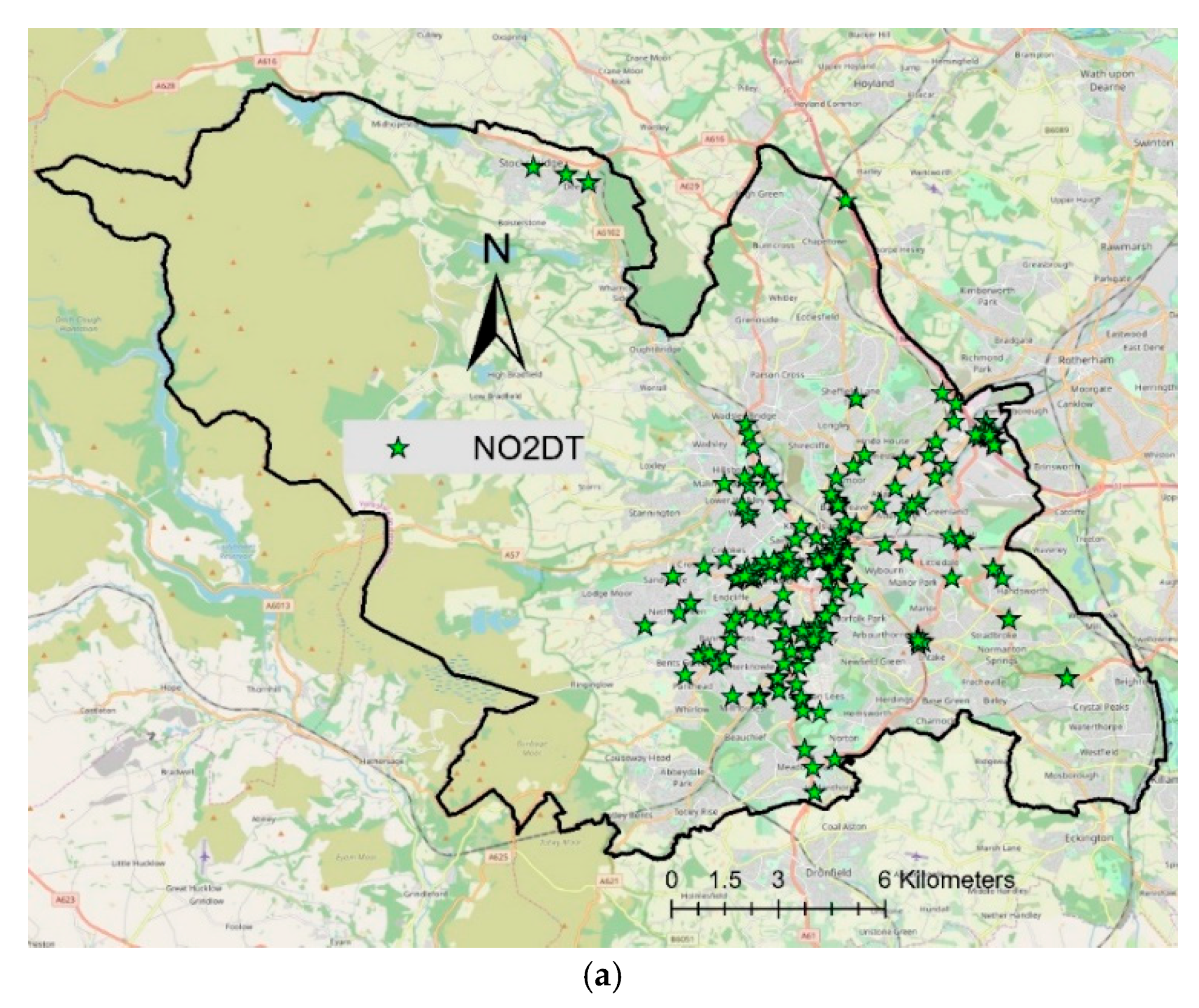
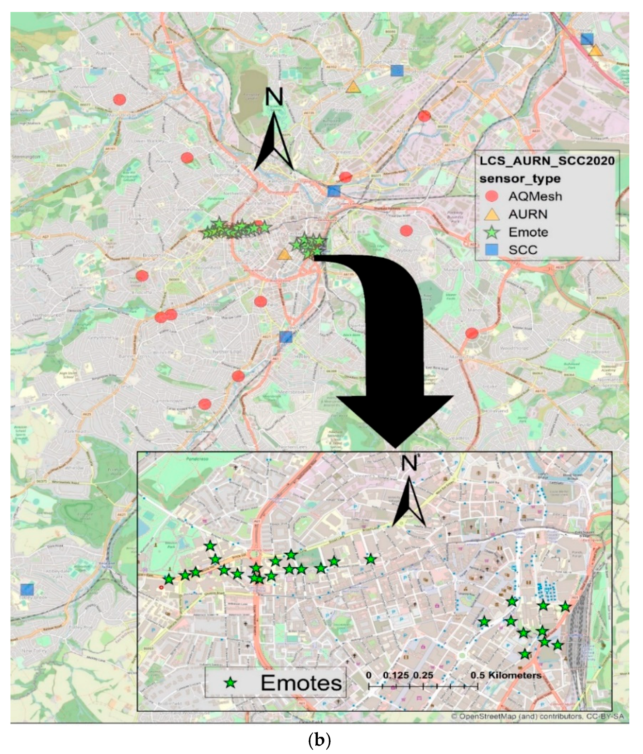
There is a large network of one hundred and eighty-eight (188) NO2 diffusion tubes (DT) in Sheffield (Figure 1a). The Urban Flows Observatory, at the University of Sheffield, has made a network of forty-one (41) low-cost sensors (LCS) which has twenty-eight (28) Envirowatch E-MOTEs and thirteen (13) AQMesh pods, providing continuous hourly data of NO2 concentrations (Figure 1b). Furthermore, in Sheffield, there are three (3) Automatic Urban and Rural Network (AURN) reference sites run by the UK Department of Environment, Food and Rural Affairs (DEFRA) and five (5) reference stations run by the Sheffield City Council (SCC) (Figure 1b). All these sensors make a multi-layer network providing NO2 data. In this paper, NO2 data for over a year (August 2019 to September 2020) are analysed. A summary of the NO2 data from the network is provided in Table 1. Further details on the network can be found in [12].
2.3. NO2 Map Estimated by Airviro
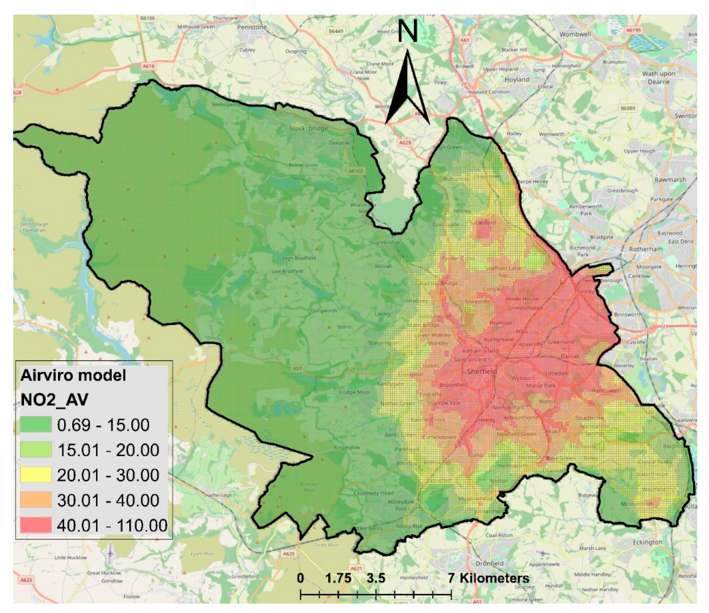
The Airviro dispersion model’s estimated map of NO2 concentrations is adopted from Munir et al. [13], who used the Airviro (version 4.01) dispersion model, which is an integrated modelling system for managing the emission database, modelling the dispersion of pollutants, and handling air quality data. Airviro is a state of the art dispersion model used by many researchers, consultants and local authorities globally for air quality modelling. Like other dispersion models, Airviro requires local topography, pollutant emissions and meteorological data to produce maps of estimated air pollutants. The Airviro model, the required inputs and produced outputs are discussed in detail in Munir et al. [13]. Munir et al. [13] estimated the map of NOx concentrations, which were converted to NO2 by analysing the ratio of NO2/NOx. The original map is given in Munir et al. [13] and the adopted map which is further analysed in this paper is shown here in Figure 2. The resulting estimated map showed hotspots of NO2 concentrations around the city centre and eastern part of the city towards the Tinsley Roundabout (M1 J34S). NO2 concentrations decrease gradually going away from the city centre, particularly towards the west and northwest of the city.
2.4. NO2 Map Estimated by LUR
The LUR map used here is adopted from Munir et al. [12]. LUR is a widely employed approach for the estimation of air pollution exposure using geographical information systems (GIS) and statistical analysis to determine the association between geographical features and measured atmospheric pollutant concentrations [15]. The LUR approach was introduced by Briggs et al. [15] and since then has been used in numerous studies around the world [16,17,18,19,20,21,22,23]. LUR models associate pollutant concentrations, such as NO2, to site-specific geographical characteristics, e.g., topography, land use, population density and altitude. The use of these variables in the regression model is known to capture small-scale variability on a city scale [24]. For more details, see [12]. The resulting map produced by the LUR model [12], employing a generalised additive model, a nonlinear regression approach, is shown in Figure 3, which is a high-resolution (100 m × 100 m) map. Figure 3 demonstrates higher levels of NO2 in the city centre, eastern side of the city and on major roads. As compared to Figure 2, here, the busy roads are successfully highlighted, showing high levels of NO2 concentrations.
2.5. Kriging and Universal Kriging
Kriging is a type of geostatistical interpolation technique based on statistical models that include statistical relationships among the measured points (autocorrelation). Kriging is a form of probabilistic and local interpolation technique. Kriging uses Gaussian processes for interpolating between various spatial points.
The kriging formula is expressed as:
where Zi(Si) is the measured value at the ith location, λi is an unknown weight for the measured value at the ith location, Zo(So) is the predicted value at the prediction location.
Simple kriging is used for stationary data if the mean is known; otherwise, ordinary kriging is used. To fuse (integrate) model estimations with measured NO2 concentrations, here, we employed the universal kriging technique, which is more advanced and capable of handling data with more than one correlated variable. In universal kriging, the additional observations of one or more covariates may lead to increased precision of the predictions. This approach enables the merging of NO2 observations from a network of sensors, with modelled values providing spatial information from the air quality models. Universal kriging, in contrast to ordinary kriging, allows the overall mean to be non-constant throughout the domain and to be a function of one or more explanatory variables [9,25]. Universal kriging is similar to kriging, with external drift and mathematically equivalent to regression kriging or residual kriging [8]. In this paper, measured values are fused with LUR and Airviro estimation using “automap” packages [14] in R programming language [26].
2.6. Model Validation
Performance of the universal kriging technique was assessed by calculating several statistical metrics. Statistical metrics used for comparing measured and estimated concentrations were factor of two (FAC2), mean bias error (MBE), mean absolute error (MAE), root mean square error (RMSE) and correlation coefficient (r). MAE and RMSE show the size of the average error; however, they do not provide information on the relative magnitude of the difference between predicted and observed values as these are based on absolute values of the difference between estimated and measured values. On the other hand, MBE describes the direction of the error bias. A negative value of MBE shows that predicted values are smaller than the observed values, showing underprediction of the model. FAC2 is the percentage of the predictions within a factor of two of the observed values and the correlation coefficient demonstrates the linear relationship between observed and estimated concentrations. For more details on these metrics see Munir et al. [12,13].
For comparison purposes, the measured data collected by different sets of sensors were split into training and testing datasets. Training dataset (75% of the data) and testing dataset (25% of the dataset) were randomly selected using “caTools” package of R programming language. After assessing the model performance, the model was retrained using the whole dataset and applied to the rest of the city where measured data were not available.
3. Results and Discussion
In this section, firstly, the measured and interpolated NO2 concentrations (µg/m3) are analysed (Section 3.1), followed by data fusion (Section 3.2), wherein model estimations are fused with measured NO2 concentrations.
3.1. Measured and Interpolated NO2 Concentrations
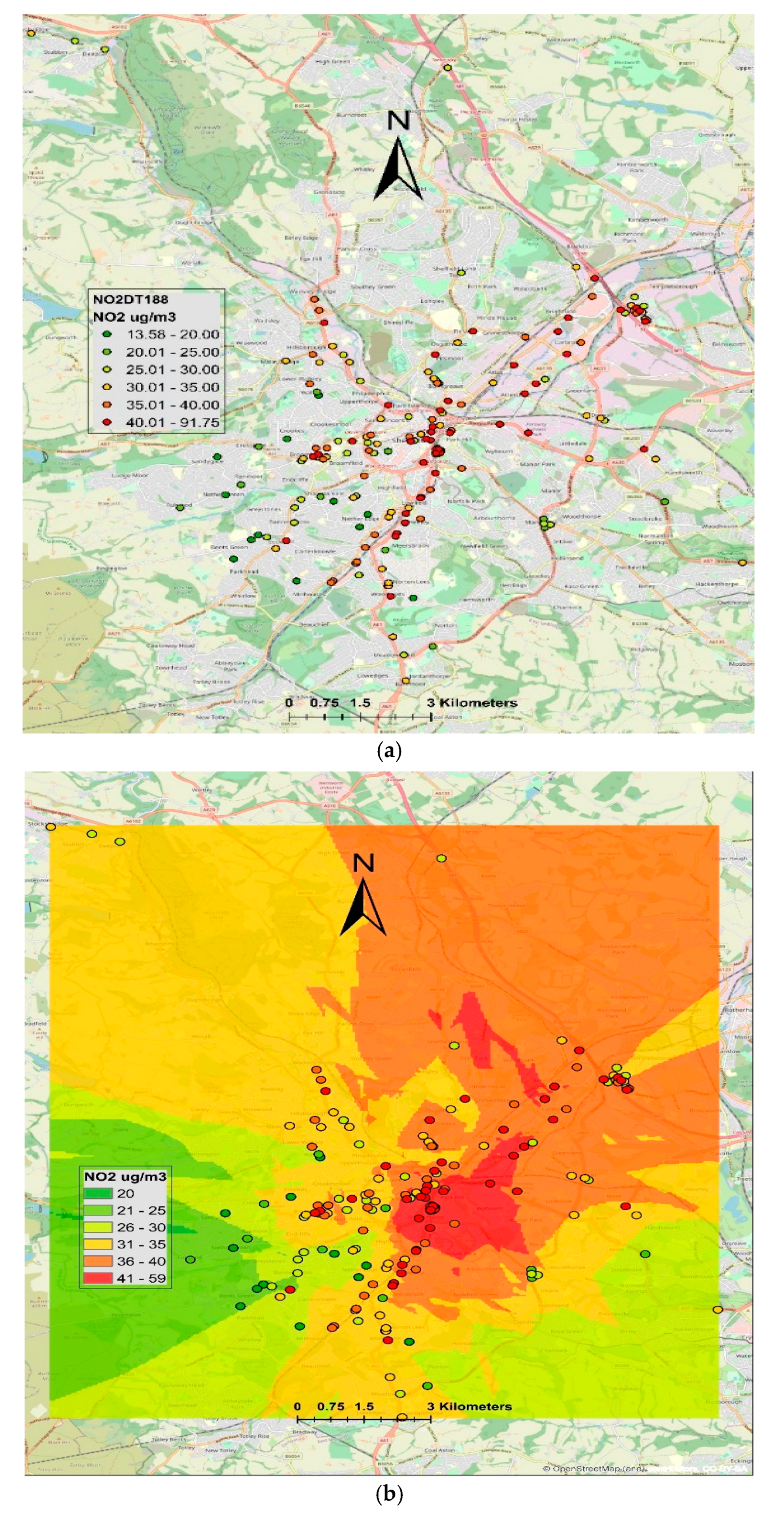
Figure 4 demonstrates both measured and interpolated NO2 concentrations for DT. Annual mean of measured NO2 concentrations (µg/m3) ranged from 13.58 to 91.75. It should be noted that the air quality limit for annual mean NO2 concentrations is 40 (µg/m3); therefore, to protect human health, annual mean NO2 levels should not exceed this level. The observed levels (Figure 4) show that the air quality limits are exceeded at several sites in the city, especially in the city centre and on main roads. These readings are only for point locations and there are large gaps between these locations. To create a continuous map, in this paper, we used ordinary kriging for predicting NO2 concentrations for the locations where measured concentrations were not available. Interpolated concentrations are shown in Figure 4b, which demonstrates that air quality standards are violated in some parts of the city centre and in the northeast of the city. However, in most of the city centre and northeast of the city, NO2 levels range from 35 to 40 (µg/m3). In the northwest and areas adjacent to the city centre, the NO2 levels ranged from 30 to 35. Deep green and light green areas mostly in the southwest part of the city show NO2 levels in the range of 20 to 30 (µg/m3), which is the area next to the Peak District National Park.
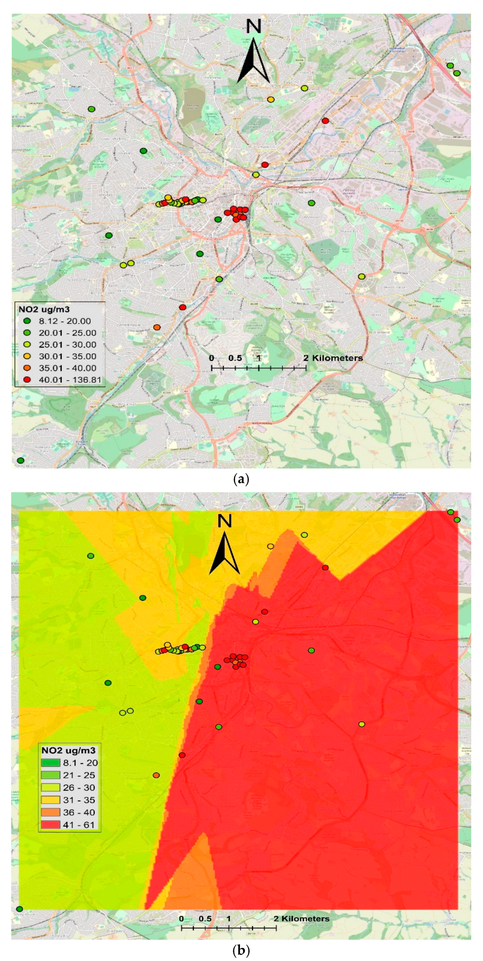
Figure 5 shows NO2 levels measured by LCS, ranging from 8.12 to 136.81 (µg/m3). Exceedances of air quality standards are mainly shown in the city centre, where 10 Envirowatch E-MOTEs were installed. However, due to the low number of sensors compared to DT, the interpolated maps are not as detailed as those produced by the DT. Envirowatch E-MOTEs installed in the city centre recorded relatively higher concentrations than the other parts of the city. Three Envirowatch E-MOTEs recorded particularly higher NO2 concentrations: (a) outside Sheffield train station next to the taxi rank, E-MOTE 904 (136.81 µg/m3), (b) Arundel Gate opposite to Genting Club, E-MOTE 732 (115.55 µg/m3), and (c) Sheaf Street/Sheaf Square adjacent to the pedestrian crossing for Howard Street, E-MOTE 903 (107.17 µg/m3). The reason for the higher concentrations is that these sites are very busy in terms of traffic flow and idling vehicles while stationary. The taxi stand (E-MOTE 904) is a good example, showing how idling vehicles contribute to air pollution in the city. E-MOTE 903 is installed next to a pedestrian crossing on a busy road. People coming out of the train station use the pedestrian crossing going towards the high street, Sheffield Hallam University and other parts of the city. The pedestrian crossing is regularly used, interrupting the traffic flow and causing congestion. When the lights turn red, road traffic stops but vehicle engines keep running. As soon as the lights turn green, all vehicles try to accelerate quickly. Therefore, idling of engine and sudden acceleration emits extra pollution, causing this location to be one of the most polluted sites. E-MOTE 732 is installed in a typical street canyon, where the road has tall buildings on both sides, hindering the dispersion of the pollutants emitted by the road traffic and causing the pollution levels to increase. The other sites in the city centre where air quality standards were exceeded are Paternoster Rows, Harmer Lane near Sheaf Street, Harmer Lane near the bus station, Arundel Gate near Surrey Street and Howard Street. Two E-MOTEs at the university campus that exceeded air quality limits were Regent Court and Broad Lane (near St. George’s Terrace). In the outskirts of the city, air quality limits were exceeded at three sites where AQMesh pods were installed: Saville Street, Abbeydale Rd and Brightside Lane. At these sites, the main source of emission is road traffic. Therefore, road traffic is the main source of emissions causing violation of AQ standards in Sheffield.
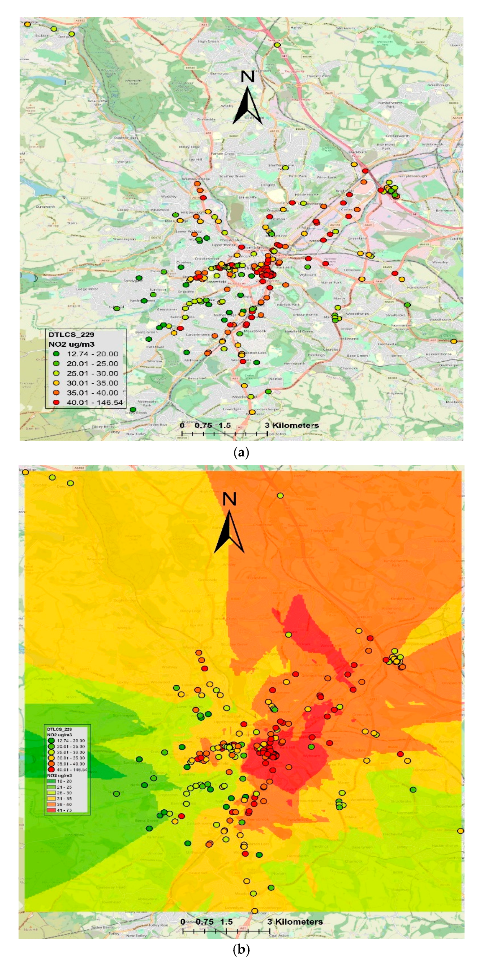
Figure 6 combines both DT and LCS, showing a more detailed map of interpolated NO2 concentrations (µg/m3). Generally, it demonstrates the same pattern as shown in Figure 4. However, in comparison to LUR (Figure 3) and Airviro models (Figure 2), the interpolated maps are less precise and less detailed. Briggs et al. [10] compared the performance of LUR with spatial interpolation methods (e.g., kriging, Triangular Interpolation Network (TIN) contouring and trend surface analysis) and reported that LUR performed much better than the interpolation techniques. The reason probably was that in urban areas, spatial variability of air pollutants was more controlled by the local emission sources, such as road traffic, rather than a smoothly varying field, which was assumed by the interpolation methods.
3.2. Data Fusion—Fusing Model Estimations with Measured Concentrations
In this section, geostatistical universal kriging was used to fuse measured NO2 concentrations with estimated NO2 concentrations. NO2 measured by DT, LCS and DTLCS are expressed as NO2-DT, NO2-LCS and NO2-DTLCS and estimation of LUR and Airviro as NO2-LUR and NO2-Airviro, respectively.
3.2.1. Fusion of NO2-LCS with NO2-Airviro and NO2-LUR
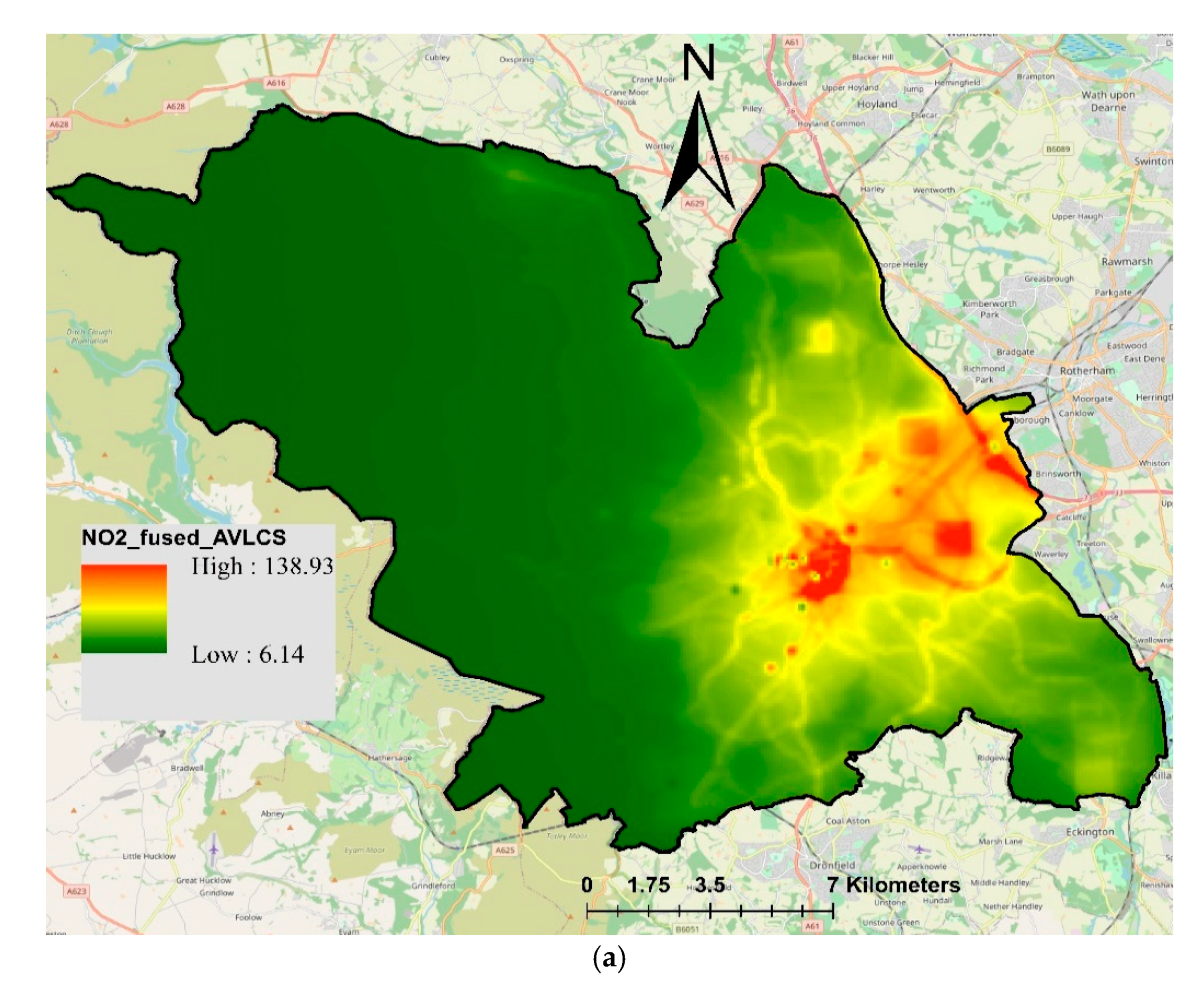
Universal kriging was used to fuse NO2-LCS with NO2-Airviro and NO2-LUR. Figure 7 presents the results of data fusion, where the fusion of NO2-Airviro with measured NO2 is presented in Figure 7a and the fusion of NO2-LUR with measured NO2 is presented in Figure 7b. The resulting fused concentrations from the integration between NO2-Airviro and NO2-LCS (Airviro-LCS) ranged from 6.14 to 138.93 µg/m3. The range of these values reflected the measured NO2-LCS concentrations (ranging from 8.11 to 136.81 µg/m3), whereas the spatial pattern followed the trend of NO2-Airviro. On the other hand, the fusion of NO2-LCS and NO2-LUR (LUR-LCS) (Figure 7b) demonstrated a slightly different pattern. The NO2 LUR-LCS ranged from 19.45 to 82.98 (µg/m3), slightly overestimating lower values and underestimating the higher values. For model validation, the fused concentrations were compared with the measured concentrations using the testing dataset (25% randomly selected) applying various statistical metrics (Table 2). Overall, NO2 LUR-LCS showed slightly better correlation (r, 0.96) and less error (RMSE, 9.09) than Airviro-LCS (r, 0.88 and RMSE, 18.16) when compared with measured concentrations. Overall, the fusion of Airviro-LCS slightly underestimated NO2 concentrations, demonstrated by the negative value of MBE (−4.14).
3.2.2. Fusion of NO2-DT with NO2-Airviro and NO2-LUR
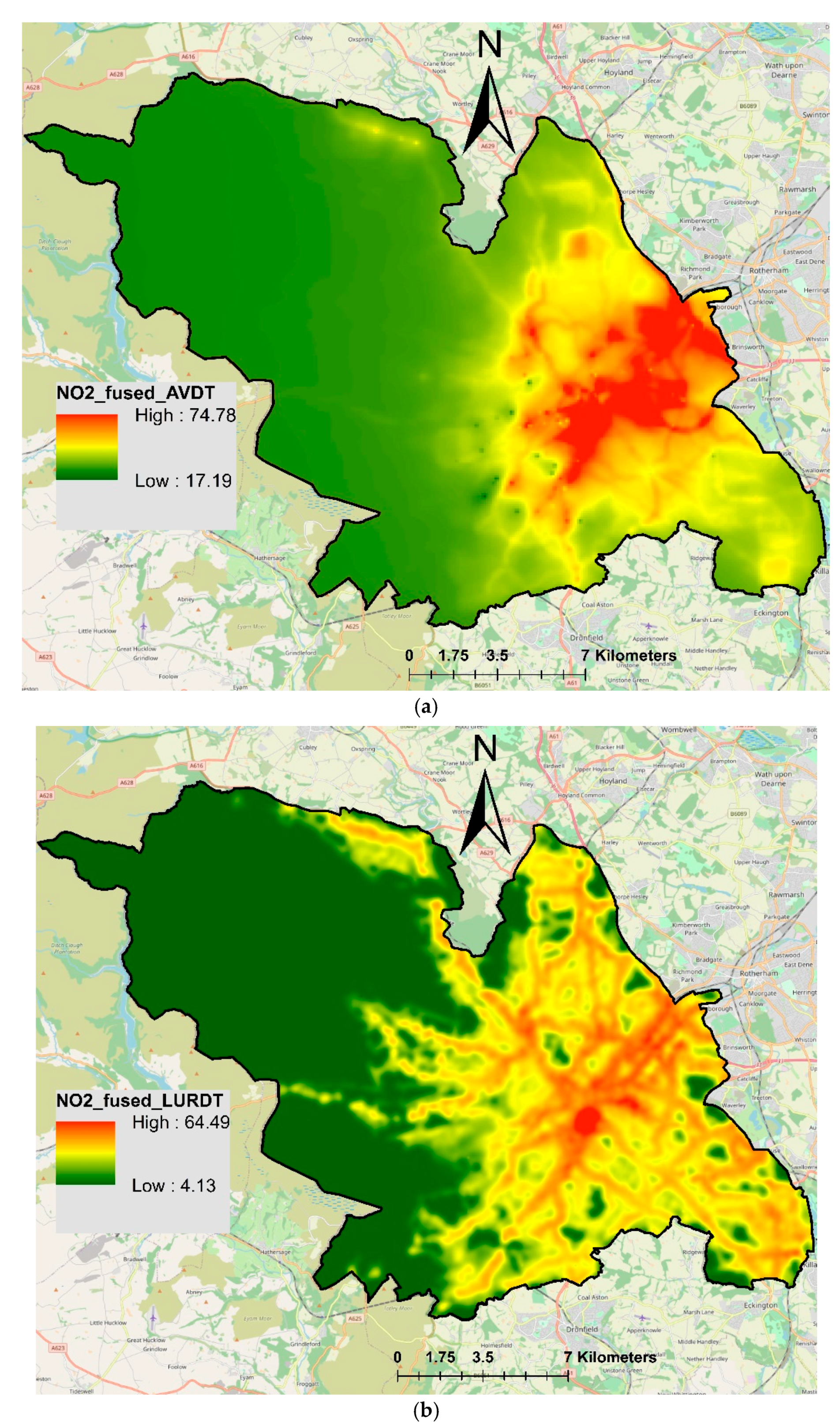
Maps produced by the fusion of NO2-DT with NO2-Airviro and NO2-LUR are presented in Figure 8, where the fusion of Airviro-DT is shown in Figure 8a and the fusion of LUR-DT is shown Figure 8b. The fused NO2 Airviro-DT ranged from 17.19 to 74.78 µg/m3. NO2-Airviro concentrations ranged from 0.69 to 110, whereas NO2-DT ranged from 13.58 to 91.75 µg/m3. Airviro-DT showed higher concentrations in the city centre, east and northeast part of the city and relatively lower concentrations in the outskirts of the city, especially towards the west and northwest part of the city. Figure 8b shows NO2 LUR-DT, which is the fusion between NO2-LUR and NO2-DT. Here, higher NO2 LUR-DT are shown in the city centre, eastern and northeastern parts. However, some busy roads and hotspots are also highlighted in some other parts of the city. NO2 LUR-DT ranged from 4.13 to 64.49 µg/m3.
Statistical metrics used to compare measured concentrations with fused concentrations (Table 2) showed the same correlation coefficient for both LUR-DT and Airviro-DT (r, 0.70). The values of other metrics, e.g., RMSE and MAE, also demonstrated negligible differences. However, visually, LUR-DT produced more detailed maps and successfully highlighted higher pollution levels on several busy roads.
3.2.3. Fusion of NO2-DTLCS with NO2-Airviro and NO2-LUR
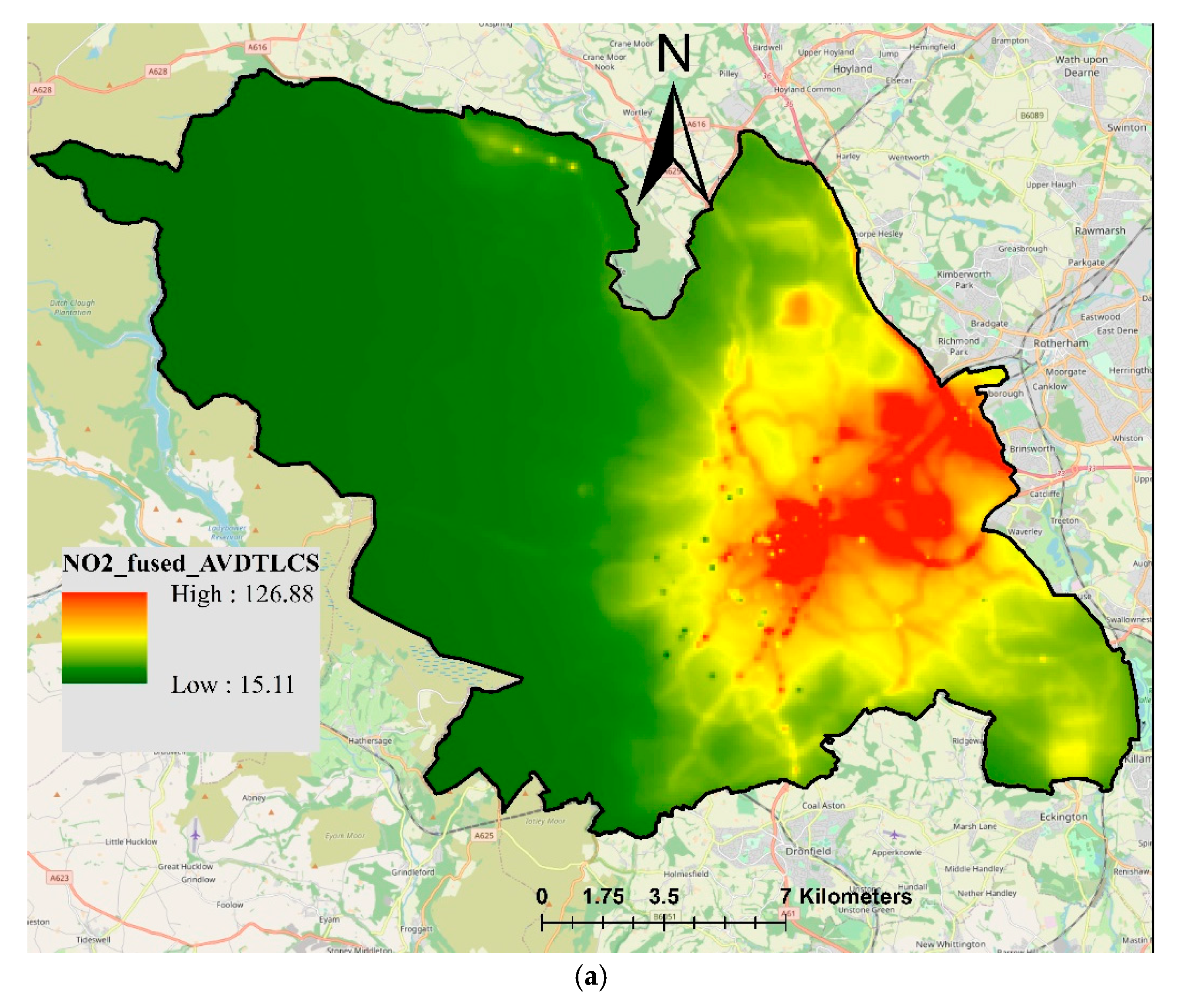
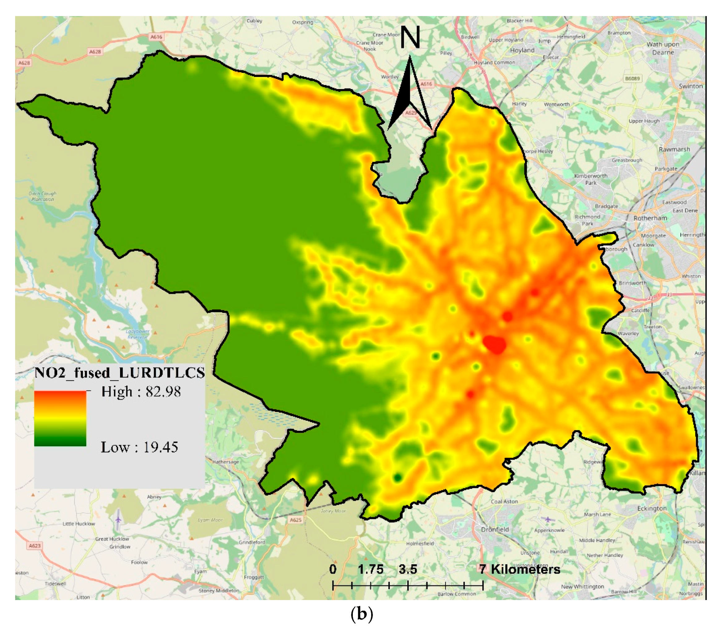
Finally, the measured NO2-DTLCS were fused with NO2-Airviro and NO2-LUR. The fused NO2 concentrations are presented in Figure 9, where the fusion of Airviro-DTLCS is shown in Figure 9a and the fusion of LUR-DTLCS is shown in Figure 9b. The resulting maps shown in Figure 9 look similar to those presented in Figure 8 in terms of spatial coverage; however, actual values and their ranges are different. Fused Airviro-DTLCS ranged from 15.11 to 126.88, whereas LUR-DTLCS ranged from 19.45 to 82.98 µg/m3. The measured NO2-DTLCS ranged from 8.12 to 136.81 µg/m3. Combining DT and LCS measurements did not improve the model performance compared to using only NO2-DT. In contrast, the values of correlation coefficient slightly decreased to 0.56 and 0.59 for Airviro-DTLCS and LUR-DTLCS, respectively. Values of RMSE were 10.42 and 10.43 for Airviro-DTLCS and LUR-DTLCS, respectively (Table 2). This shows that increasing the number of sensors will not necessarily improve the output of the data fusion, especially if the sensors are not the same type.
The values of measured NO2 concentrations are reflected in fused values, whereas the spatial trend is determined by the model values. The fused maps provided better coverage and more realistic concentrations than the interpolated maps using ordinary kriging. Data fusion also improved the NO2-Airvrio and NO2-LUR maps, producing more realistic maps based on both measured and estimated concentrations. Overall, the fusion of LUR with measured concentrations produced better results than the Airviro model in terms of correlation coefficient, RMSE and MAE.
In this study, different monitoring and modelling approaches were used to produce high-resolution spatial maps of NO2 concentrations in urban areas. Air quality monitoring is the more accurate source of data for assessing air pollutant levels. However, the air quality monitoring network cannot be dense enough to provide measured data for each spatial point in the whole city. Therefore, different modelling approaches (e.g., spatial interpolations, dispersion models and LUR models) are required to predict air quality information between monitoring stations. These models, in addition to measured data, use emission data, meteorology data, traffic characteristics, population data and land use characteristics. One of the issues with air quality modelling is its level of uncertainty, which is significantly higher than the measured data [27]. This is where data fusion techniques play their role by combining measured and modelled data in such a way to improve the spatiotemporal resolution of the measured data and accuracy of the modelled data.
Huang et al. [28] applied data fusion techniques to integrate measured and model estimation over North Carolina, USA. In contrast to this study, Huang et al. [28] analysed the levels of several air pollutants which were PM2.5, CO, NOx, NO2 and five particulate species (organic carbon, elemental carbon, and sulphate, nitrate and ammonium ions). They reported that the application of data fusion reduced biases in the model estimation. The correlation coefficient for the cross-validation test was 0.91 in Huang et al. [28], which was less than this study (r-value 0.96). Gressent et al. [29] analysed air quality data from low-cost sensors and integrated them with the estimation of ADMS-Urban in France. In contrast to this study, which uses annual NO2 concentrations, Gressent et al. [29] used hourly data and estimated PM10 concentrations for 29 November 2018 from 7 a.m. to 7 p.m. They used external drift kriging, which is similar to universal kriging, and reduced the bias from 8% to 2% when considering LCS observations instead of the model alone. Schneider et al. [9] employed geostatistics methodology to fuse NO2 concentrations obtained from a network of low-cost sensors (AQMesh) and EPISODE dispersion model. EPISODE is a 3-D Eulerian/Lagrangian dispersion model providing atmospheric air pollutant forecasts at urban and regional scales. For more details on the EPISODE model [30]. Schneider et al. [9] evaluated the geostatistics universal kriging methodology for fusing both measured and predicted data of NO2 in Oslo, Norway during January 2016. Results showed that the fusing method was able to produce realistic hourly NO2 concentrations, which inherited the spatial trend of the pollutant from the EPISODE model. Furthermore, fused data were compared to measured data from a reference instrument and results showed reasonably good resemblance between measured and fused data, with R2 value of 0.89 and mean squared error of 14.3 µg/m3. Their model showed slightly inferior performance in comparison to this study, with r-value 0.96 and RMSE 9.09. Furthermore, Schneider et al. [9] had used a shorter time-period of one month and fewer sensors as compared to this study, which used NO2 data for a whole year from more sensors.
Most of the data fusion techniques mentioned above are applied on city scales. However, several researchers have also applied the data fusion approaches to air quality data on a country level [31] or global level [32]. Liang et al. [31] developed a data fusion method and compared the outputs with kriging-with-external-drift (KED) and the chemistry module from WRF-Chem (Weather Research and Forecast Model with Chemistry Module). KED is a type of universal kriging that takes into account the local trend of the variable (e.g., air pollutant concentrations) as well as external drift (a spatial trend) when minimising the variance of estimation [8]. Both KED and WRF-Chem were used to estimate daily PM2.5 levels in 10-km grid cells in China during 2013. The estimated concentrations from both KED and WRF-Chem were then fused with measured observations. For fusion, a simple linear regression model was applied between the observed and estimated concentrations for both KED and chemistry models in turns. The regression coefficients obtained from the regression model were used to adjust the predicted concentrations. The performance of the models was evaluated, and KED and regression data fusion methods showed better performance in terms of R2 value of 0.95 and 0.94, respectively, as compared to the value of 0.51 for WARF-Chem model. Shaddick et al. [32], employing a Bayesian hierarchical modelling framework, estimated that 92% of the world’s population lived in areas where air pollution levels exceeded the World Health Organization’s air quality guidelines. However, the results of these investigations carried out on a country or global level are not comparable with studies conducted on a city level.
4. Conclusions
In this paper, different modelling and data fusion techniques were employed to analyse the spatial variability of NO2 concentrations (µg/m3) in the city of Sheffield. NO2 was monitored by 188 DT, 41 low-cost sensors, 3 AURN and 5 SCC monitoring stations. The main difference between LCS and reference sensors is that LCS are cheaper, compact and their measurements are less reliable, whereas AURN and SCC use reference sensors which are much more expensive and reliable. However, the reference AQMN is sparse, having fewer AQMS, which are not enough for understanding the spatial variability of NO2 in Sheffield. Therefore, the networks of LCS and DT were used for analysing the spatial variability of NO2 concentrations and validating the models. Air quality standards were exceeded at several locations in Sheffield, particularly in the city centre and on some busy roads, where annual mean NO2 levels were higher than 40 µg/m3. The highest levels of NO2 were recorded by the Envirowatch E-MOTE installed next to the Sheffield train station taxi rank (136.81 µg/m3), followed by the Sheaf Street/Sheaf Square pedestrian crossing (115.56 µg/m3) and Arundel Gate (107.17 µg/m3).
Three modelling approaches were used to produce maps of NO2 concentrations in Sheffield: (a) geostatistical kriging interpolation, (b) Airviro dispersion modelling, and (c) LUR based on the generalised additive model. Measured NO2 concentrations were fused with the estimated concentrations using universal kriging, which is an advanced kriging technique that is employed for data having more than one correlated variable. Six sets of measured and estimated NO2 data were fused: (i) Fusion of NO2-Airviro with NO2-LCS; (ii) Fusion of NO2-Airviro with NO2-DT; (iii) Fusion of NO2-Airviro with NO2-DTLCS; (iv) Fusion of NO2-LUR with NO2-LCS; (v) Fusion of NO2-LUR with NO2-DT; and (vi) Fusion of NO2-LUR with NO2-DTLCS. Fused NO2 were compared with measured concentrations in terms of different statistical metrics including FAC2, r, RMSE, MAE and MBE. Maps produced by the fusion of NO2-LCS and NO2-LUR produced better results, with an r-value of 0.96, followed by the fusion of NO2-Airviro with NO2-LCS, with an r-value of 0.88. Fused maps developed by universal kriging provided better spatial coverage and similarity with measured concentrations than the ordinary kriging interpolation, Airviro and LUR models. Fused maps combining measured and estimated concentrations produced more realistic concentrations and provided better spatial coverage.
This study presents a geostatistical universal kriging approach for fusing measured and estimated NO2 concentrations to improve our understanding of small-scale spatial variability in NO2 concentrations in Sheffield. This approach adds value to both measured and estimated values: the measured concentrations are improved by predicting spatiotemporal gaps, whereas the modelled concentrations are improved by constraining them with observed data. The main findings of this study are: (a) The universal kriging approach was capable of estimating realistic NO2 concentration maps from the fusion of measured and modelled concentrations. The fused NO2 concentrations inherited spatial patterns of the pollutant from the model estimations and adjusted the modelled values using the measured concentrations. (b) A huge number of sensors are required to provide reasonable spatial coverage at a city level, which is too expensive. Spatial modelling (e.g., dispersion model and LUR model) and data fusion approaches can provide city-level maps by integrating pollutant concentrations measured by the AQMS with modelled concentrations. (c) According to Schneider et al. [9], the accuracy of the data fusion depends on the number of sensors, their spatial distribution, their uncertainty and the accuracy of the estimated values to be fused with measured values. Here, we showed that in addition, the accuracy of the data fusion also depends on the uniformity of the sensors, meaning that using the same type of sensors can result in better accuracy. Increasing the number of sensors will not necessarily improve the model outputs, especially if sensors are not of the same type. For example, maps produced by the fusion of NO2-LCS with NO2-LUR (r-value 0.96) and NO2-Airviro (r-value 0.88) produced better results than when both NO2-DT and NO2-LCS were used together and fused with NO2-LUR or NO2-Airviro, when the r-values decreased to 0.59 and 0.56, respectively.
The uniqueness of this study is that it uses estimated NO2 concentrations from two sources—a dispersion model and a land use regression model—and measured NO2 concentrations from three sources: diffusion tubes, reference sensors and low-cost sensors. The study applies geostatistical universal kriging for data fusion and produces high-resolution maps of NO2 in Sheffield.
Limitations/weaknesses: (a) NO2 diffusion tube data were downloaded from the Sheffield City Council website; we do not know which correction factors were applied before they were published online. (b) Low-cost sensors have their limitations and are not as accurate as reference sensors. The data from the low-cost sensors are postprocessed by the manufacturers with the aim of correcting cross-interferences as well as the effects of temperature and relative humidity. The AQMesh pods include an O3-filtered NO2 sensor from Alphasense, which is designed to reject O3 and hence eliminate cross-sensitivity issues. However, none of these sensors was collocated with the reference sensor in the field; therefore, we could not develop and apply correction factors.
In the future, we aim to apply this approach to high-resolution spatiotemporal data (e.g., hourly data on city scale) to further improve spatiotemporal estimation of NO2 concentrations. Furthermore, the data fusion work would be done in as near to real time as possible in the form of an app, so as to provide public health advice.
Author Contributions
Conceptualization, S.M.; Formal analysis, S.M.; Funding acquisition, M.M. and D.C.; Methodology, S.M.; Supervision, M.M. and D.C.; Visualization, S.M.; Writing—original draft, S.M. All authors have read and agreed to the published version of the manuscript.
Funding
This research was funded by the Engineering and Physical Sciences Research Council (EPSRC) (grant number—EP/R512175/1) and Siemens plc. The APC was paid by UKRI/EPSRC.
Institutional Review Board Statement
Not applicable.
Informed Consent Statement
Not applicable.
Data Availability Statement
Acknowledgments
We would like to express our thanks to the Engineering and Physical Sciences Research Council (EPSRC), grant number—EP/R512175/1 and Siemens plc for funding this project. We are also thankful to Sheffield City Council for providing NO2 diffusion tubes data.
Conflicts of Interest
All the authors declare no conflict of interest.
References
- Public Health England. Guidance, Air pollution: Applying All Our Health. 2020. Available online: https://www.gov.uk/government/publications/air-pollution-applying-all-our-health/air-pollution-applying-all-our-health (accessed on 19 January 2021).
- Fan, Z.; Pun, V.C.; Chen, X.C.; Hong, Q.; Tian, L.; Ho, S.S.H.; Lee, S.C.; Tse, L.A.; Ho, K.F. Personal exposure to fine particles (PM2.5) and respiratory inflammation of common residents in Hong Kong. Environ. Res. 2018, 164, 24–31. [Google Scholar] [CrossRef]
- WHO. Review of Evidence on Health Aspects of Air Pollution-REVIHAAP Project: Final Technical Report. World Health Organziation Regional Office for Europe. 2013. Available online: https://www.euro.who.int/__data/assets/pdf_file/0004/193108/REVIHAAP-Final-technical-report-final-version.pdf (accessed on 28 January 2021).
- Landrigan, P.J. Air pollution and health. Lancet Public Health 2016, 2, 4–5. [Google Scholar] [CrossRef] [Green Version]
- DEFRA. Improving Air Quality in the UK Tackling Nitrogen Dioxide in Our Towns and Cities, UK Overview Document, December 2015. Available online: https://www.gov.uk/government/uploads/system/uploads/attachment_data/file/486636/aq-plan-2015-overview-document.pdf (accessed on 9 April 2020).
- Xie, X.; Semanjski, I.; Gautama, S.; Tsiligianni, E.; Deligiannis, N.; Rajan, R.T.; Pasveer, F.; Philips, W. A Review of Urban Air Pollution Monitoring and Exposure Assessment Methods. ISPRS Int. J. Geo. inf. 2017, 6, 389. [Google Scholar] [CrossRef] [Green Version]
- Briggs, D.J. The Role of GIS: Coping with Space (And Time) in Air Pollution Exposure Assessment. J. Toxicol. Environ. Health 2005, 68, 1243–1261. [Google Scholar] [CrossRef]
- Hengl, T.; Heuvelink, G.; Stein, A. Comparison of Kriging with External Drift and Regression-Kriging; ITC Technical note; International Institute for Geo-Information Science and Earth Observation (ITC): Enschede, The Netherlands, 2003. [Google Scholar]
- Schneider, P.; Castell, N.; Vogt, M.; Dauge, F.R.; Lahoz, W.A.; Bartonova, A. Mapping urban air quality in near real-time using observations from lowcost sensors and model information. Environ. Int. 2017, 106, 234–247. [Google Scholar] [CrossRef] [PubMed]
- Briggs, D.J.; de Hough, C.; Gulliver, J.; Wills, J.; Elliott, P.; Kingham, S.; Smallbone, K. A regression-based method for mapping traffic-related air pollution: Application and testing in four contrasting urban environments. Sci. Total Environ. 2000, 253, 151–167. [Google Scholar] [CrossRef]
- Castanedo, F. A Review of Data Fusion Techniques. Sci. World J. 2013, 2013, 1–19. [Google Scholar] [CrossRef] [PubMed]
- Munir, S.; Mayfield, M.; Coca, D.; Mihaylova, L.S. A nonlinear land-use regression approach for modelling NO2 concentrations in urban areas—Using data from low-cost sensors and diffusion tubes. Atmosphere 2020, 11, 736. [Google Scholar] [CrossRef]
- Munir, S.; Mayfield, M.; Coca, D.; Mihaylova, L.S.; Osammor, O. Analysis of air pollution in urban areas with Airviro dispersion model—A Case Study in the City of Sheffield, United Kingdom. Atmosphere 2020, 11, 285. [Google Scholar] [CrossRef] [Green Version]
- Hiemstra, P. Automatic Interpolation Package. “Automap”, Version 1.0-14, a Package for R Programming Language. 2015. Available online: https://cran.r-project.org/web/packages/automap/automap.pdf (accessed on 28 January 2021).
- Briggs, D.J.; Collins, S.; Elliott, P.; Fischer, P.; Kingham, S.; Lebret, E.; Pryl, K.; van Reeuwijk, H.; Smallbone, K.; van der Veen, A. Mapping urban air pollution using GIS: A regression-based approach. Int. J. Geogr. Inf. Sci. 1997, 11, 699–718. [Google Scholar] [CrossRef] [Green Version]
- Beelen, R.; Hoek, G.; Fischer, P.; van den Brandt, P.A.; Brunekreef, B. Estimated long-term outdoor air pollution concentrations in a cohort study. Atmos. Environ. 2007, 41, 1343–1358. [Google Scholar] [CrossRef]
- Eeftens, M.; Beelen, R.; de Hoogh, K. Development of land use regression models for PM2.5, PM2.5 absorbance, PM10 and PM coarse in 20 European Study areas; results of the ESCAPE project. Environ. Sci. Technol. 2012, 46, 11195–11205. [Google Scholar] [CrossRef] [PubMed]
- Hoek, G.; Beelen, R.; De Hoogh, K.; Vienneau, D.; Gulliver, J.; Fischer, P. A review of land-use regression models to assess spatial variation of outdoor air pollution. Atmos. Environ. 2008, 42, 7561–7578. [Google Scholar] [CrossRef]
- Lee, J.-H.; Wu, C.-F.; Hoek, G.; De Hoogh, K.; Beelen, R.; Brunekreef, B.; Chan, C.-C. Land use regression models for estimating individual NOx and NO2 exposures in a metropolis with a high density of traffic roads and population. Sci. Total. Environ. 2014, 472, 1163–1171. [Google Scholar] [CrossRef]
- Muttoo, S.; Ramsay, L.; Brunekreef, B.; Beelen, R.; Meliefste, K.; Naidoo, R.N. Land use regression modelling estimating nitrogen oxides exposure in industrial south Durban, South Africa. Sci. Total Environ. 2017, 610–611, 1439–1447. [Google Scholar] [CrossRef]
- Rahman, M.M.; Yeganeh, B.; Clifford, S.; Knibbs, L.D.; Morawska, L. Development of a land use regression model for daily NO2 and NOx concentrations in the Brisbane metropolitan area, Australia. Environ. Modell. Softw. 2017, 95, 168–179. [Google Scholar] [CrossRef] [Green Version]
- Stedman, J.; Vincent, K.; Campbell, G.; Goodwin, J.; Downing, C. New high resolution maps of estimated background ambient NOx and NO2 concentrations in the U.K. Atmos. Environ. 1997, 31, 3591–3602. [Google Scholar] [CrossRef]
- Ryan, P.H.; LeMasters, G.K.; Biswas, P.; Levin, L.; Hu, S.; Lindsey, M.; Bernstein, D.I.; Lockey, J.; Villareal, M.; Hershey, G.K.K.; et al. A comparison of proximity and land use regression traffic exposure models and wheezing in infants. Environ. Health Perspect. 2007, 115, 278–284. [Google Scholar] [CrossRef] [Green Version]
- Ryan, P.H.; LeMasters, G.K. A review of land-use regressionmodels for characterizing intraurban air pollution exposure. Inhal. Toxicol. 2007, 19 (Suppl. 1), 127–133. [Google Scholar] [CrossRef] [Green Version]
- Goovaerts, P. Geostatistics for Natural Resources Evaluation; Applied Geostatistics Series; Oxford University Press: Oxford, UK, 1997; ISBN 0-19-511538-4. [Google Scholar]
- R Core Team. R: A Language and Environment for Statistical Computing; R Foundation for Statistical Computing: Vienna, Austria, 2019; Available online: https://www.R-project.org/ (accessed on 28 January 2021).
- Denby, B.; Garcia, V.; Holland, D.M.; Hogrege, C. Integration of air quality modeling and monitoring data for enhanced health exposure assessment. Air Waste Manag. Assoc. 2009, 10, 46–49. [Google Scholar]
- Huang, R.; Zhai, X.; Ivey, C.E.; Friberg, M.D.; Hu, X. Using Air Quality Model-Data Fusion Methods for Developing Air Pollutant Exposure Fields and Comparison with Satellite AOD-Derived Fields: Application over North Carolina, USA. In Air Pollution Modeling and Its Application XXV; Mensink, C., Kallos, G., Eds.; Springer Proceedings in Complexity Book Series; Springer: Cham, Switzerland, 2018. [Google Scholar] [CrossRef]
- Gressent, A.; Malherbe, L.; Colette, A.; Rollin, H.; Scimia, R. Data fusion for air quality mapping using low-cost sensor observations: Feasibility and added-value. Environ. Int. 2020, 143, 105965. [Google Scholar] [CrossRef] [PubMed]
- Slordal, L.H.; Walker, S.E.; Solberg, S.S. The Urban Air Dispersion Model EPISODE Applied in AirQUIS 2003—Technical Description; NILU—Norwegian Institute for Air Research: Kjeller, Norway, 2003. [Google Scholar]
- Liang, F.; Gao, M.; Xiao, Q.; Carmichael, G.R.; Pan, X.; Liu, Y. Evaluation of a data fusion approach to estimate daily PM2.5 levels in North China. Environ. Res. 2017, 158, 54–60. [Google Scholar] [CrossRef] [PubMed] [Green Version]
- Shaddick, G.; Thomas, M.L.; Green, A.; Brauer, M.; van-Donkelaar, A.; Burnett, R. Data integration model for air quality: A hierarchical approach to the global estimation of exposures to ambient air pollution. J. R. Stat. Soc. Ser. Appl. Stat. 2018, 67, 231–253. [Google Scholar] [CrossRef]
Figure 1.
Showing the locations of DT, LCS (both AQMesh pods and Envirowatch E-MOTEs), AURN and SCC monitoring sites in Sheffield: (a) DT locations; (b) AURN, SCC and LCS locations.
Figure 1.
Showing the locations of DT, LCS (both AQMesh pods and Envirowatch E-MOTEs), AURN and SCC monitoring sites in Sheffield: (a) DT locations; (b) AURN, SCC and LCS locations.


Figure 2.
Spatial variability of annual mean modelled NO2 in Sheffield. Maps were developed using Airviro model (modified from [13]).
Figure 2.
Spatial variability of annual mean modelled NO2 in Sheffield. Maps were developed using Airviro model (modified from [13]).

Figure 3.
Maps of annual mean modelled NO2 (µg/m3) estimated by LUR model in Sheffield. Modified from [12].
Figure 3.
Maps of annual mean modelled NO2 (µg/m3) estimated by LUR model in Sheffield. Modified from [12].

Figure 4.
Showing point and interpolated NO2 levels from DT network: (a) NO2 concentrations (µg/m3) from DT, and (b) interpolated NO2 concentrations (µg/m3) using ordinary kriging.
Figure 4.
Showing point and interpolated NO2 levels from DT network: (a) NO2 concentrations (µg/m3) from DT, and (b) interpolated NO2 concentrations (µg/m3) using ordinary kriging.

Figure 5.
Showing point and interpolated NO2 levels from LCS network: (a) NO2 concentrations (µg/m3) from LCS, (b) interpolated NO2 concentrations (µg/m3) using ordinary kriging.
Figure 5.
Showing point and interpolated NO2 levels from LCS network: (a) NO2 concentrations (µg/m3) from LCS, (b) interpolated NO2 concentrations (µg/m3) using ordinary kriging.

Figure 6.
Showing point and interpolated NO2 levels from both DT and LCS: (a) NO2 concentrations (µg/m3) from both 188 DT and LCS, and (b) interpolated NO2 concentrations (µg/m3) using ordinary kriging.
Figure 6.
Showing point and interpolated NO2 levels from both DT and LCS: (a) NO2 concentrations (µg/m3) from both 188 DT and LCS, and (b) interpolated NO2 concentrations (µg/m3) using ordinary kriging.

Figure 7.
Resulting map of fused NO2 concentrations (µg/m3) using universal kriging techniques: (a) NO2 Airviro-LCS; (b) NO2 LUR-LCS.
Figure 7.
Resulting map of fused NO2 concentrations (µg/m3) using universal kriging techniques: (a) NO2 Airviro-LCS; (b) NO2 LUR-LCS.


Figure 8.
Resulting maps of fused NO2 concentrations (µg/m3) using universal kriging techniques: (a) NO2 Airviro-DT; (b) NO2 LUR-DT.
Figure 8.
Resulting maps of fused NO2 concentrations (µg/m3) using universal kriging techniques: (a) NO2 Airviro-DT; (b) NO2 LUR-DT.

Figure 9.
Resulting map of fused NO2 concentrations (µg/m3) using universal kriging techniques: (a) Airviro-DTLCS; (b) LUR-DTLCS.
Figure 9.
Resulting map of fused NO2 concentrations (µg/m3) using universal kriging techniques: (a) Airviro-DTLCS; (b) LUR-DTLCS.


Table 1.
Summary of annual mean NO2 concentrations (µg/m3) measured by diffusion tubes (DT), automatic urban and rural network (AURN), Sheffield City Council (SCC) and low-cost sensors (LCS) (AQMesh and Envirowatch) in Sheffield (August 2019 to September 2020).
Table 1.
Summary of annual mean NO2 concentrations (µg/m3) measured by diffusion tubes (DT), automatic urban and rural network (AURN), Sheffield City Council (SCC) and low-cost sensors (LCS) (AQMesh and Envirowatch) in Sheffield (August 2019 to September 2020).
| Metrics | DT NO2 | AURN | SCC | AQMesh/Envirowatch E-MOTE |
|---|---|---|---|---|
| Minimum | 13.58 | 19.09 | 8.12 | 12.69 |
| 1st Quartile | 28.29 | 21.00 | 24.05 | 25.08 |
| Median | 33.77 | 22.90 | 24.62 | 34.23 |
| Mean | 34.23 | 24.69 | 21.53 | 38.70 |
| 3rd Quartile | 40.00 | 27.50 | 25.02 | 42.36 |
| Maximum | 91.75 | 32.09 | 25.86 | 136.81 |
| Standard Deviation | 9.65 | 6.68 | 7.53 | 27.69 |
| Number of Sensors | 188 | 3 | 5 | 41 |
Table 2.
Showing the values of different statistical metrics calculated by comparing fused and measured NO2 concentrations based on randomly selected testing dataset (train/test cross-validation). FAC2, MBE, MAE, RMSE and r stand for factor of two, mean biased error, mean absolute error, root mean squared error, and correlation coefficient.
| Metrics | Airviro-LCS | LUR-LCS | Airviro-DT | LUR-DT | Airviro-DTLCS | LUR-DTLCS |
|---|---|---|---|---|---|---|
| FAC2 | 1 | 1 | 1 | 1 | 0.98 | 0.96 |
| MBE | −4.14 | 1.44 | 1.56 | 1.40 | 1.08 | 2.24 |
| MAE | 12.79 | 7.99 | 5.81 | 5.29 | 8.20 | 3.73 |
| RMSE | 18.16 | 9.09 | 7.18 | 6.74 | 10.42 | 10.43 |
| R | 0.88 | 0.96 | 0.70 | 0.70 | 0.56 | 0.59 |
Publisher’s Note: MDPI stays neutral with regard to jurisdictional claims in published maps and institutional affiliations. |
© 2021 by the authors. Licensee MDPI, Basel, Switzerland. This article is an open access article distributed under the terms and conditions of the Creative Commons Attribution (CC BY) license (http://creativecommons.org/licenses/by/4.0/).
Share and Cite
MDPI and ACS Style
Munir, S.; Mayfield, M.; Coca, D. Understanding Spatial Variability of NO2 in Urban Areas Using Spatial Modelling and Data Fusion Approaches. Atmosphere 2021, 12, 179. https://0-doi-org.brum.beds.ac.uk/10.3390/atmos12020179
AMA Style
Munir S, Mayfield M, Coca D. Understanding Spatial Variability of NO2 in Urban Areas Using Spatial Modelling and Data Fusion Approaches. Atmosphere. 2021; 12(2):179. https://0-doi-org.brum.beds.ac.uk/10.3390/atmos12020179
Chicago/Turabian StyleMunir, Said, Martin Mayfield, and Daniel Coca. 2021. "Understanding Spatial Variability of NO2 in Urban Areas Using Spatial Modelling and Data Fusion Approaches" Atmosphere 12, no. 2: 179. https://0-doi-org.brum.beds.ac.uk/10.3390/atmos12020179
Note that from the first issue of 2016, this journal uses article numbers instead of page numbers. See further details here.