
Geo-Hydrological Events and Temporal Trends in CAPE and TCWV over the Main Cities Facing the Mediterranean Sea in the Period 1979–2018


1
Istituto di Ricerca per la Protezione Idrogeologica (IRPI) del Consiglio Nazionale delle Ricerche (CNR), Strada delle Cacce 73, 10135 Turin, Italy
2
Centro Internazionale di Ricerca in Monitoraggio Ambientale CIMA Research Foundation, via A. Magliotto 2, 17100 Savona, Italy
*
Author to whom correspondence should be addressed.
Atmosphere 2022, 13(1), 89; https://0-doi-org.brum.beds.ac.uk/10.3390/atmos13010089
Submission received: 8 December 2021
/
Revised: 1 January 2022
/
Accepted: 5 January 2022
/
Published: 6 January 2022
(This article belongs to the Special Issue Geo-Hydrological Extreme Events in the Mediterranean and Black Sea Areas)
Abstract
:The Mediterranean region is regarded as the meeting point between Europe, Africa and the Middle East. Due to favourable climatic conditions, many civilizations have flourished here. Approximately, about half a billion people live in the Mediterranean region, which provides a key passage for trading between Europe and Asia. Belonging to the middle latitude zone, this region experiences high meteorological variability that is mostly induced by contrasting hot and cold air masses that generally come from the west. Due to such phenomenon, this region is subject to frequent intensive precipitation events. Besides, in this complex physiographic and orographic region, human activities have contributed to enhance the geo-hydrologic risk. Further, in terms of climate change, the Mediterranean is a hot spot, probably exposing it to future damaging events. In this framework, this research focuses on the analysis of precipitation related events recorded in the EM–DAT disasters database for the period 1979–2018. An increasing trend emerges in both event records and related deaths. Then a possible linkage with two meteorological variables was investigated. Significant trends were studied for CAPE (Convective Available Potential Energy) and TCWV (Total Column Water Vapor) data, as monthly means in 100 km2 cells for 18 major cities facing the Mediterranean Sea. The Mann–Kendall trend test, Sen’s slope estimation and the Hurst exponent estimation for the investigation of persistency in time series were applied. The research provides new evidence and quantification for the increasing trend of climate related disasters at the Mediterranean scale: recorded events in 1999–2018 are about four times the ones in 1979–1998. Besides, it relates this rise with the trend of two meteorological variables associated with high intensity precipitation events, which shows a statistically significative increasing trend in many of the analysed cities facing the Mediterranean Sea.
Keywords:
flood; flash flood; Mediterranean Sea; CAPE; TCWV; geo-hydrological event; temporal trend; Hurst exponent1. Introduction
The Mediterranean area shows a complex hydro-meteorological cycle [1] with important socio-economic implications for a wide region, encompassing southern Europe, northern Africa and the Middle East [2,3,4,5]. It provides a unique atmospheric, oceanic and hydrological coupled system, due to its geomorphological setting: a nearly closed sea surrounded by urbanized coasts and mountains from which numerous rivers originate.
The Mediterranean hydro-meteorological cycle is significantly influenced by both mid-latitude and sub-tropical climate dynamics. Severe weather events, including heavy precipitation leading to flash-flooding episodes, occur during the fall season; conversely severe cyclogenesis associated with strong winds and large sea waves occur during winter. Besides, summer heat waves and droughts accompanied by forest fires, regularly affect the Mediterranean region causing heavy damage and loss of human life.
The Mediterranean region has been identified as one of the two main climate change hot spots at a global scale, together with north eastern European regions, suggesting that climate is especially responsive to global climate change in this area [6]. Large decreases in mean precipitation and increases in precipitation variability during the dry (warm) season are expected, as well as large increases in temperature (from +1.4 to +5.8 °C in 2100).
Llasat et al., (2010) [7] constructed a database of high-impact floods and flash floods in Mediterranean countries and their results suggested that the spatial distribution of the different kinds of floods is neither homogeneous in the region, nor stationary over time; instead, it shows a clear distinction between the western and the eastern Mediterranean, with a major concentration of events in the former region. In the western Mediterranean, Spain and Italy suffer for the highest flood frequency, but the material and economic damages are particularly high in Italy. Floods are less frequent in southern Mediterranean countries (northern Africa) but are usually catastrophic with a very high number of casualties.
Events in Liguria (13 deaths in October 2011 and 6 deaths in November 2011), in western Attica in Greece (24 deaths in November 2017), in the Balearic Islands (13 deaths in October 2018), in southern France (15 deaths in October 2018), in Italy (36 deaths in October–November 2018), in Greece (4 deaths in September 2020 for Medicane Ianos) and in central-southern Mediterranean (Tunisia, Algeria, Malta, and Italy, 7 deaths in October 2021 for Medicane Apollo) show that flood-related mortality remains a major concern in Mediterranean countries prone to flash floods. Along these lines, Petrucci et al. [5] and Vinet et al. [8] created the Mediterranean Flood Fatality Database (MEFF DB) for six Mediterranean regions/countries: Catalonia (Spain), Balearic Islands (Spain), southern France, Calabria (Italy), Greece, and Turkey, and covering the period 1980–2018. Petrucci et al. [5] focused on the profile of victims and the circumstances of the accidents and showed that in most cases they were killed while travelling by car. Vinet et al. [8] addressed the spatial distribution of flood mortality through a geographical information system (GIS) at different spatial scales and identified a negative mortality gradient between the western and the eastern parts of the Mediterranean Sea and identified the south of France as the most affected region.
The capability to predict such high-impact hydro-meteorological events, despite the significant progress of the last decade, remains weak because of the contribution of very fine-scale processes as well as their non-linear interactions with the larger scale ones. Advances in the identification of the predominant processes and particularly of their interactions at different scales are needed to better forecast these events and reduce uncertainties on the prediction of their evolution (e.g., frequency, intensity) and socio-economic impacts under the future climate.
In this framework, several studies have been devoted to gaining a deeper understanding of the relationships between high-impact hydro-meteorological events and key controlling phenomena at synoptic and mesoscales. Reale et al. [9] investigated, with the aid of a water vapour back-trajectory technique, the large-scale source of moisture for a series of floods in the Mediterranean area and they found that the additional contribution of Atlantic hurricanes, in terms of moisture advection, can be important for these severe hydro-meteorological phenomena. Molini et al. [10] classified severe rainfall events over the Mediterranean area as, either long-lived and spatially distributed (Type I) if lasting more than 12 h and larger than 50 × 50 km2, or brief and localized (Type II), if having a shorter duration or a smaller spatial extent. Their work examined the hypothesis that the two types of events were associated with different dynamical regimes distinguished by different degrees of control of convective precipitation by the synoptic-scale flow. Values of the convective adjustment timescale, τc, shorter than 6 h indicate convection that is responding rapidly to the synoptic environment (equilibrium, Type I events), while slower timescales indicate that other, presumably local, factors dominate, thus resulting in highly localized and unpredictable convection phenomena (non-equilibrium, Type II events).
Pinto et al. [11] focused on rainfall annual maxima for five reference durations (1, 3, 6, 12, and 24 h) over 200 stations in the north-western Italy area. They initially classified a day as an extraordinary rainfall day when a regional threshold, calculated on the basis of a two-components with extreme values, is exceeded for at least one of the stations. Subsequently, a clustering procedure that took into account the different rainfall durations was applied to identify about 160 events. It was found that clusters including the most intense events were characterized by strong and persistent upper air troughs inducing, not only moisture advection from the North Atlantic into the Western Mediterranean, but also strong northward flow towards the southern Alpine ranges.
Grazzini et al. [12] investigated a wide number of extreme precipitation events (EPEs) occurring between 1979 and 2015 in northern-central Italy. The EPEs were subdivided into three categories (Cat1, Cat2, Cat3) according to thermodynamic conditions over the affected region. It was found that the three categories differed not only in terms of the local meteorological conditions, but also in terms of the evolution and properties of precursor Rossby wave packets (RWP).
In this research, the 40-year period between 1979 and 2018 was investigated. Both on the ground geo-hydrological events and CAPE (Convective Available Potential Energy) and TCWV (Total Content in Water Vapor) climatological variables were analysed, with the aim of probing possible trends, supporting further climate studies and providing adaptation policies. CAPE and TCWV variables are two important severe weather indicators as they capture two important ingredients for severe weather occurrence, namely instability and moisture availability. CAPE is directly related to the atmospheric instability and thus to the maximum potential vertical speed within an updraft; thus, higher values indicate greater potential for severe weather, and observed values in thunderstorm environments may often exceed 1000 joules per kilogram (J/kg), and in extreme cases may exceed 5000 J/kg. The availability of significant TCWV amounts, together with atmospheric stability indices such as CAPE, provides a good indicator for severe weather phenomena [13]. Although the TCWV does not represent the vertical structure of moisture, it describes horizontal gradients of integrated water vapour content. Therefore, the TCWV is one of the critical variables used by forecasters when severe weather conditions are expected [14]. Statistical techniques have been used to spatially analyse the satellite-collected monthly time series of CAPE and TCWV values, which are correlated with extreme rain events.
2. Material and Methods
2.1. Physiography
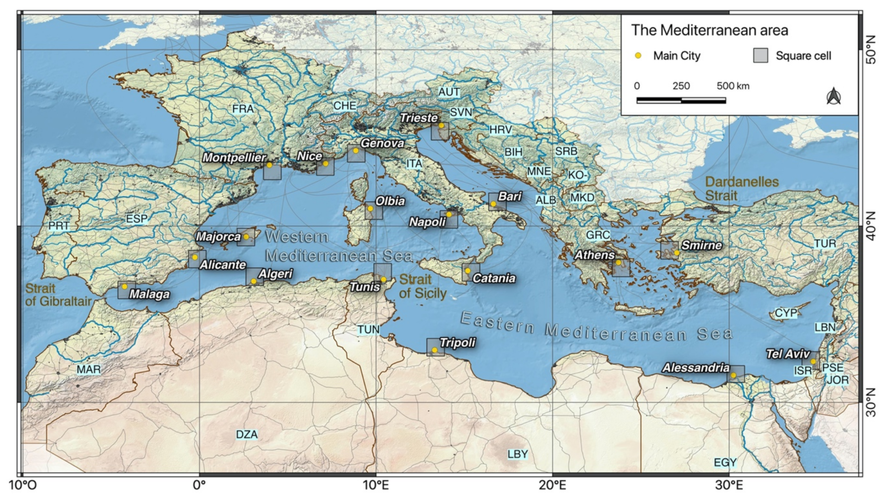
The research was conducted in the Mediterranean Sea region (lat. 26° N–51° N, long. 10° W–37° E), which shares land and sea borders with different countries (Figure 1). The Mediterranean Sea, whose floor reaches the maximum depth of about 4900 m between Italy and Greece, is divided into the Western and the Eastern areas (Figure 1) by the Strait of Sicily [15]. The two parts are then divided into submarine basins, from west to east (Figure 2): the Alboran Sea, the Balearic Sea, the Ligurian Sea, the Tyrrhenian Sea, the Adriatic Sea, the Ionian Sea, the Aegean Sea, the Sea of Crete and the Levantine Sea. The whole Mediterranean Sea is linked to the Atlantic Sea and to the Black Sea respectively through the two narrow straits of Gibraltar and Dardanelles. The limited size and depth of these two thresholds strongly limits the water exchange between the three seas.
Southern Europe, north Africa and the Middle East border the Mediterranean Sea respectively to the north, south and east. In this region, the landscape and climatic conditions are very variable, ranging from mountains to flat desert land and from alpine to arid. The general physiography of the Mediterranean is related to the geodynamic evolution that built the Alpine belt. Being part of the global Alpine-Himalayan orogenic belt [16] it comprises: the Pyrenes, between Spain and France, the Apennine belt along the Italian peninsula, the Balkan belt and the Turkish plateau. These high and complex reliefs were shaped by the endogenous and exogenous processes and play a crucial role in the regional climate and hydrology. The seasonal precipitation regime and the geomorphologic-geologic setting, together with the land cover, determine the hydrology of the Mediterranean catchments, which are small in area compared to those of a continental scale [3]. This situation, together with a low rainfall in the north African territories, results in a relatively small freshwater contribution to the Sea. In addition, the large variability of landscape and of the climate determine river flow regimes across the Mediterranean area. As a result, floods and severe weather-related events are considered common natural hazards [17].
2.2. Meteorological-Climatic Settings
The Mediterranean area is characterized by a climate that mainly reflects its position in the global atmospheric system and the complex distribution of land bordering the relatively small Mediterranean Sea. The area is affected by both high-pressure subtropical systems and by the westerly wind belt [18]. According to the seasonal cycle, one prevails over the other, influencing the climate: in winter it is typically wet and mild, while in summer it is hot and dry. Such a climate condition is defined as Mediterranean, type Cs in the Koppen classification [19] and is subdivided into continental (CSa) and maritime (Csb) [17].
The landmass distribution, with the Mediterranean Sea elongated along the Parallels and a complex topography, greatly influences the climate in the studied area; the climate, therefore, varies greatly at a local scale, from a temperate oceanic one to the north to the arid one of the south. An altitude effect determines the presence of boreal and polar climate types in areas of higher mountains.
The Mediterranean area is seasonally exposed to the influence of cold air masses coming from the extra-tropical belt, or of the warm ones originated in the subtropical belt. This alternation and mutual interaction, and the interaction between the warm sea surface and the air masses coming from the Atlantic, strongly affects the meteorological condition of the whole area. Further, it is responsible for the high cyclogenesis of the region and of the typical convective instability, which is strongly influenced by the interaction with the diffuse presence of mountain barriers. Within the cyclogenesis period between 1998 and 2001, there were about 2910 cyclones per year in the west zone and 2248 in the east zone [20]. The worst affected areas, both in summer and in winter, were the lands facing the Alboran Sea, the Balearic Sea, the Gulf du Lion area, the Ligurian and northern Tyrrhenian Sea, the northern Adriatic Sea and the southern Turkish coastline and Cyprus [17]. The highest cyclogenesis per year was recorded in the Gulf of Genoa, in the Ligurian Sea, and close to Cyprus.
2.3. Data
To evaluate the geo-hydrologic events that impacted the studied area between 1979 and 2018, the EM–DAT, the International Disaster Database, was accessed [24]. Data were extracted according to the following disaster criteria:
- Group: natural;
- Subgroup: hydrological, meteorological;
- Type: flood, landslide, storm;
- Subtype: coastal flood, convective storm, extra-tropical storm, flash flood, riverine flood, landslide, mudslide.
Data were collated by country according to Figure 1 and the relative caption. Event positions were geocoded according to the textual location data in the database. In many cases, different events were located in the same position (Figure 2) as, for example, in Corsica, or many events in Italy, France and Spain: this was due to an imprecise location because of the large scale of the positioning, or because events repeatedly affected the same area. A total of 454 events and 6170 related deaths were considered. The EM–DAT database collects data from UN agencies, non-governmental organizations, insurance companies, research institutes and press agencies from the year 1900.
CAPE—Convective Available Potential Energy and TCWV—Total Content in Water Vapor data were collected from the Copernicus Climate Change Service—Climate Data Store [25] and sampled at 0.25° cell resolution. The used database was the ERA5 monthly averaged reanalysed data on single levels from 1979 to 2018: the two large amounts of data were collected in a NetCDF format. The extracted series were analysed using the spatial mean values for the 100 km2 areas around some of the major cities facing the Mediterranean Sea, which have been periodically hit by geo-hydrological events.
2.4. Methods
Geo-hydrological events and death toll data were analysed at a monthly, yearly, and decadal frequency. The sub-type categories, distribution over the time period, and the per country toll, were considered in order to reveal any trends for the events in time and space.
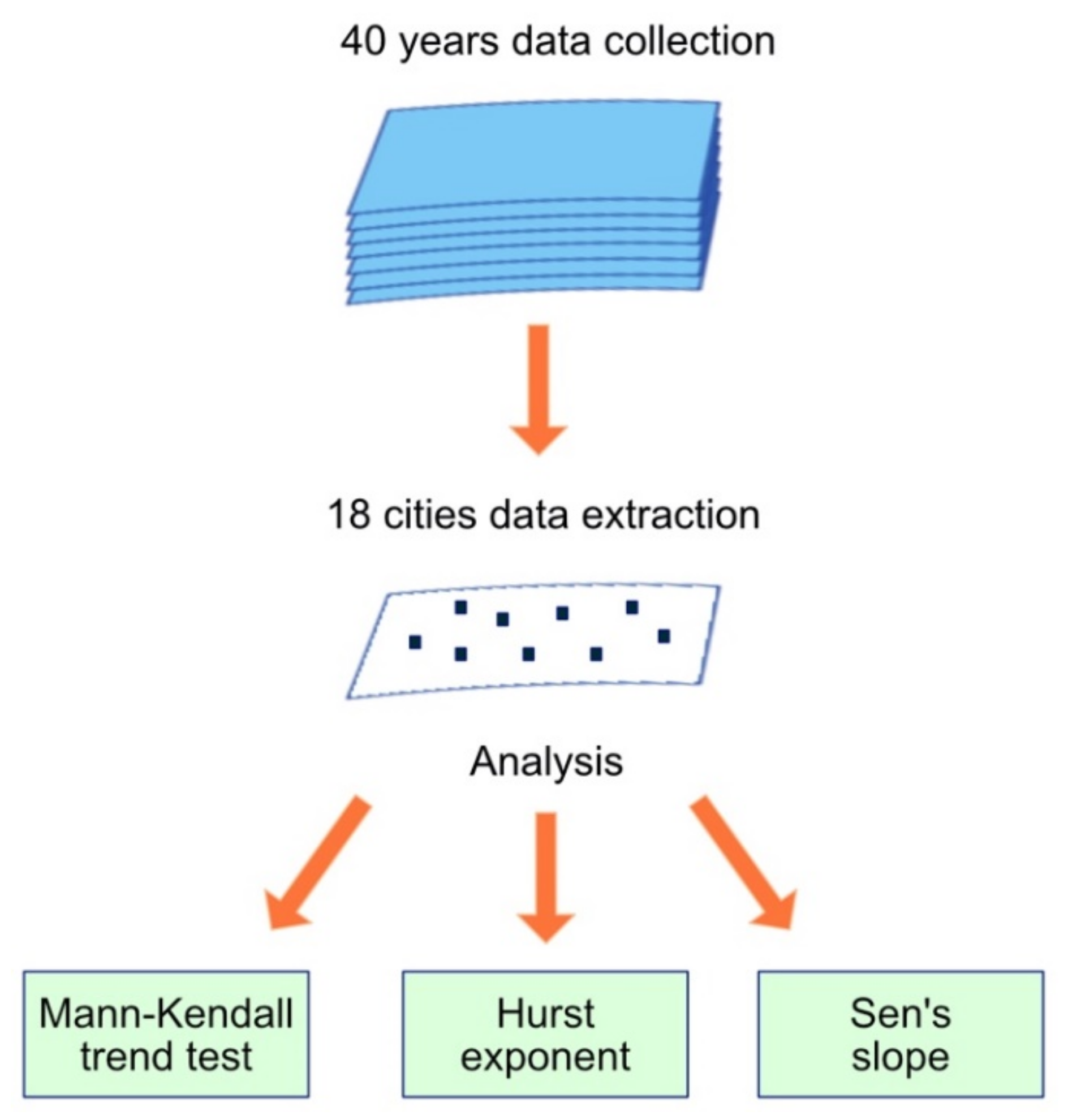
The same purpose of exploring trends in time and space dimensions drove analyses for CAPE and TCWV data, following the procedure in Figure 3. The results were achieved through the following steps:
- Data preparation;
- Methods selection;
- Analytical algorithm application;
- Results presentation.
QGis software was used in step 1: the monthly 1979–2018 series of mean CAPE and TCWV values were computed over 100 km2 square cells surrounding the selected cities. Three methods for temporal trends investigation were applied to the monthly series, as described in the next paragraphs. The Excel RealStat module [26] was used to compute the Mann–Kendall test and Sen slope estimator; a dedicated spreadsheet was used for the Hurst exponent calculation. The three methods are described below.
2.4.1. Mann–Kendall Trend Test
The non-parametric Mann–Kendall trend test [27,28] is commonly used to assess the statistical trend significance in hydro-meteorologic time series [29,30,31,32]. The test statistic S for a (x1…xn) time series is defined as follows:
The variance is given by:
where n denotes the amount of data in the series, m the number of tied groups (i.e., sets of sample data having the same value) and ti the number of ties of extent i.
When the size of the series is n > 10, the standard normal test statistic is:
The Z sign denotes the trend: positive values correspond to increasing trend and negative values correspond to decreasing trend. In this research, a 5% significance level was used.
2.4.2. Sen’s Slope Estimator
The non-parametric Sen’s slope estimator [33] is based on a linear model and relies on considering all the couple of points in a series and the relative fitting line slopes; the Sen’s slope is defined as the median of all the computed slopes. This estimator is insensitive to outliers and is a more robust method than the linear regression one.
All the possible slopes are computed for every couple of values (xi, xj) at times i and j (i > j):
Then the Sen’s slope is computed as the median of the Qk values.
2.4.3. Hurst Exponent
It was introduced by Hurst, based on Einstein’s theory on Brownian motion [34] to investigate the problem of reservoir control of the Aswan dam reservoir [35]. The Hurst exponent method [36] gives an estimation of a time series autocorrelation and it is a powerful tool to study persistence and long-range dependence [37,38]. It is widely used in many research fields, from climate science [39,40,41,42] to hydrology and water resources [38,43,44] and economics [35,45]. In this research, the rescaled range (R/S) analysis [36] provides the estimation of the Hurst exponent. Given a time series the following quantities are defined:
where is range series, is the standard deviation series, is the mean series, is the accumulative deviation series and t is the number of data items. Then considering that the R/S statistic asymptotically follows the relation the scaling exponent H may be obtained through a linear regression procedure for increasing time extents, and H . If the process is a Brownian motion, then H = 0.5, if it is persistent H > 0.5 and anti-persistent for H < 0.5; for a linear trend H = 1.
3. Results
3.1. Geo-Hydrological Events
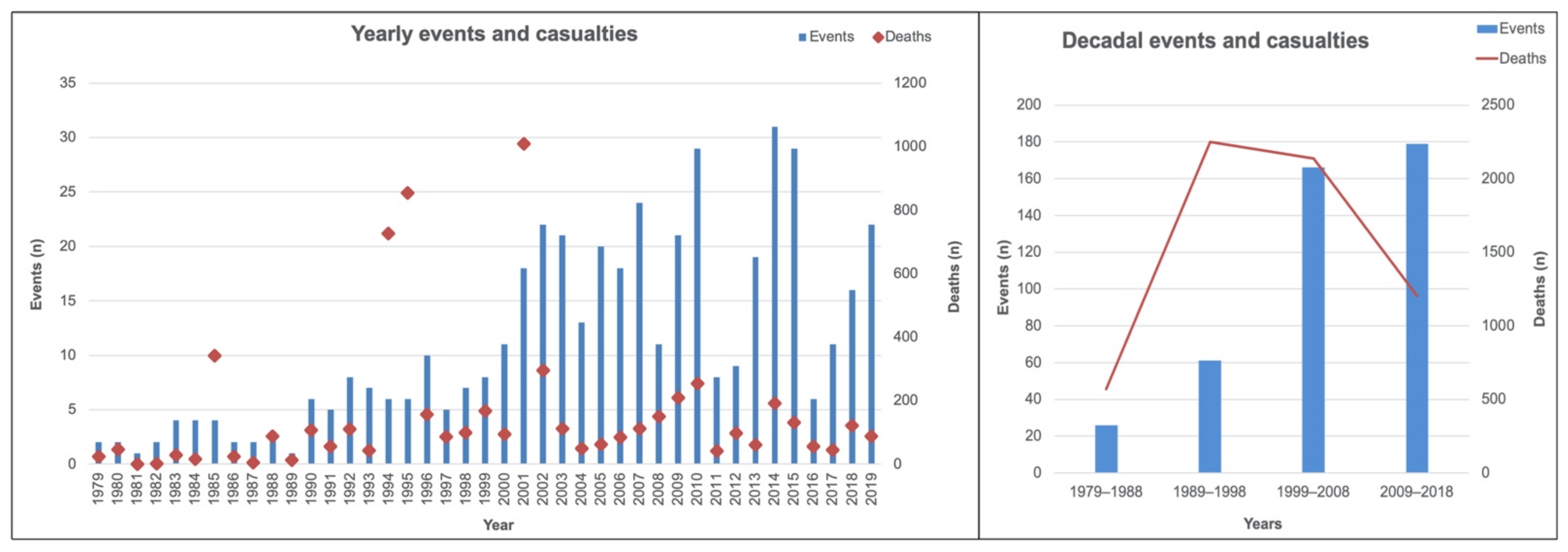
The EM–DAT database analysis allowed the assessment of the geo-hydrological severe weather events over the 40-year period for the countries facing or close to the Mediterranean Sea: both the events, count per year and per month, and the related casualties were considered. The number of events per year (Figure 4) increased from 1990 and then accelerated further after 2000. In the period 2011–2018, the recorded events were affected by a high variability: the low counts in 2011, 2012 and 2016 were interposed by the highest counts, those for 2014 and 2015. The general trend is more evident in Figure 4, where data were grouped by decade: events in the last two decades were about six times as frequent as those in 1979–1988, and about three times those in 1989–1998.
Considering the number of fatalities, no trend emerges over the 40-year period: the highest count occurred in the 1989–1998 decade, when in 1994 and 1995, two highly devastating floods affected Egypt with 600 victims and Morocco with 730 victims, respectively. A similar high magnitude flood with associated landslides and mudflows occurred in 2001 in Algeria, causing 930 deaths. These death tolls strongly affected the totals in those years.
The high victim number in 1985 had a different origin, as it was caused by the tailing pond dam break that occurred after heavy rains in the mountains of northern Italy (Stava, Trento province) killing 324. In this case, even if it was induced by rainfall, the event was highly affected by human activity, as the dam break occurred after the lack of proper maintenance.
Observing the distribution of events by month and by year (Table 1), the increase in the count, that emerged previously, shows its annual nature: the few events in the first decade (from 1 to 4) occurred occasionally in any season, but starting from the second decade, the event frequency rose sparsely throughout the whole year. This effect was exacerbated as the number of events increased, then the many events per year from 2001 to 2018 were distributed over the whole year, but mainly in fall and winter.
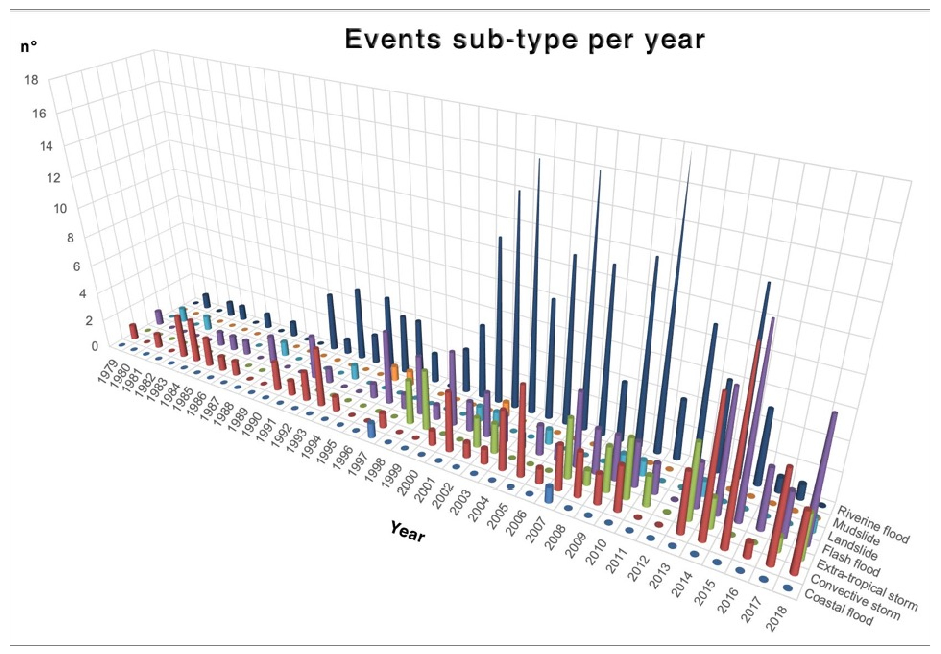
Figure 5 shows the event sub-type distribution by year between 1979 and 2018, following their definition in Section 2.3. It clearly shows the increase in numbers of riverine and flash floods, and extra-tropical and convective storms, from the year 2000 compared to their lower incidence in the previous periods. The increase in event number is most strongly evident for flash floods and convective storms in the last decade 2009–2018. Landslide events, which are large landslides, appear to be quite equally distributed over the whole studied period, while the incidence of coastal storms and mudslides was occasional.
Finally, the distribution of the total number of events and deaths per country is presented in Table 2. It shows the impact of the serious floods already mentioned that affected Egypt, Morocco and Algeria, which caused the high death tolls in those countries. On the other hand, Italy, Turkey, France and Spain also account for a high number of events and associated deaths. Figure 2 shows a thematic map of the collected severe geo-hydrological events in the studied countries that confirms the above-mentioned incidence and their spatial distribution: it appears that there is a high frequency along the coastlines of Morocco, Algeria, Israel, Lebanon, with the highest number in the Balkan peninsula. In the remaining countries, the events appear scattered over the territory with some areas of major occurrence around the Gulf du Lion and Ligurian Sea and in northern Portugal.
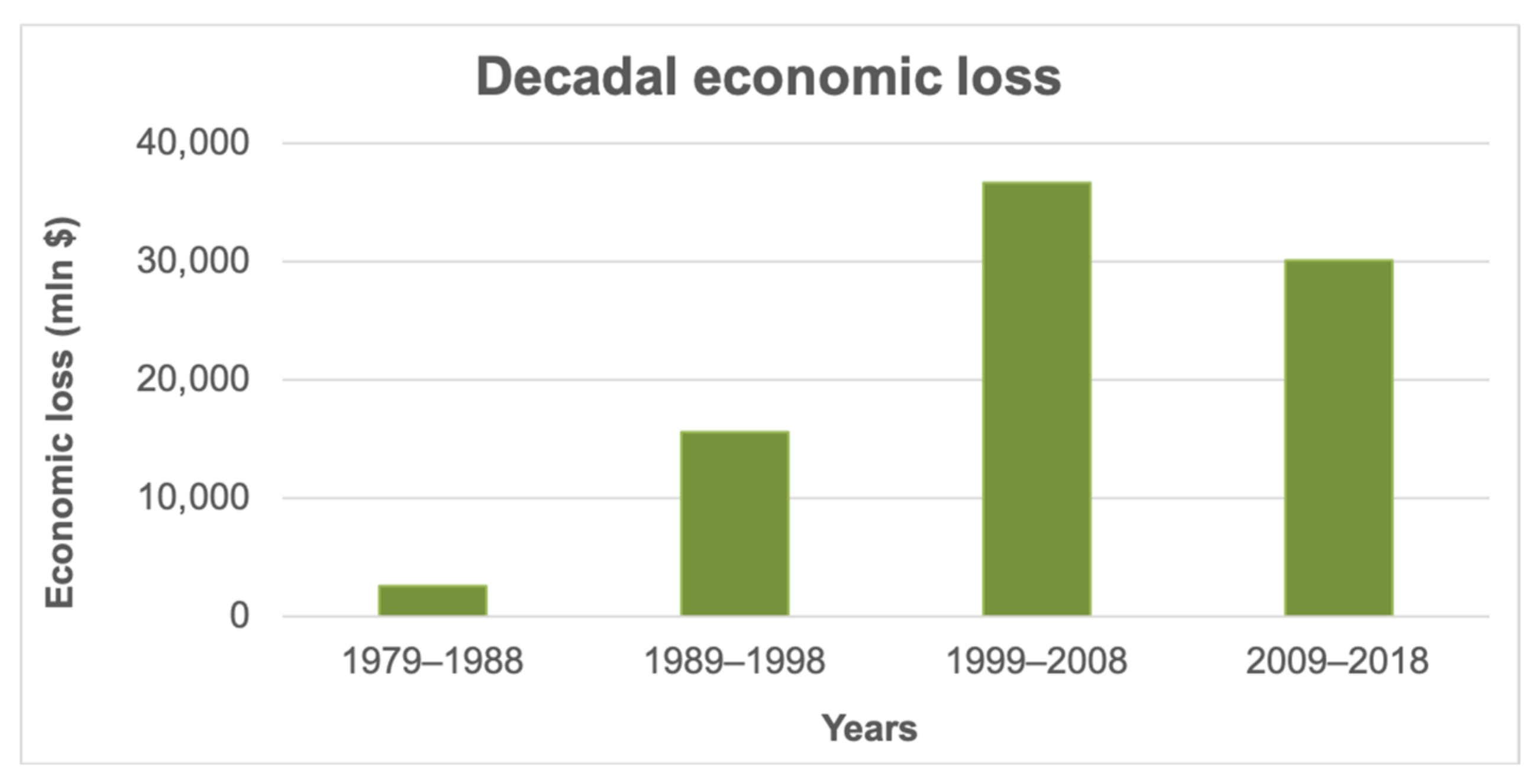
Lastly, the EM–DAT database includes the total damage (economic loss) per event, which were grouped by decade in Figure 6. Despite the lack of some data for all decades and its sparseness over the whole investigated area, it reveals a coherent increasing trend correlated with events and related deaths: the economic loss in 1999–2008 and 2009–2018 is significatively higher than in the previous two decades.
3.2. Convective Available Potential Energy—CAPE
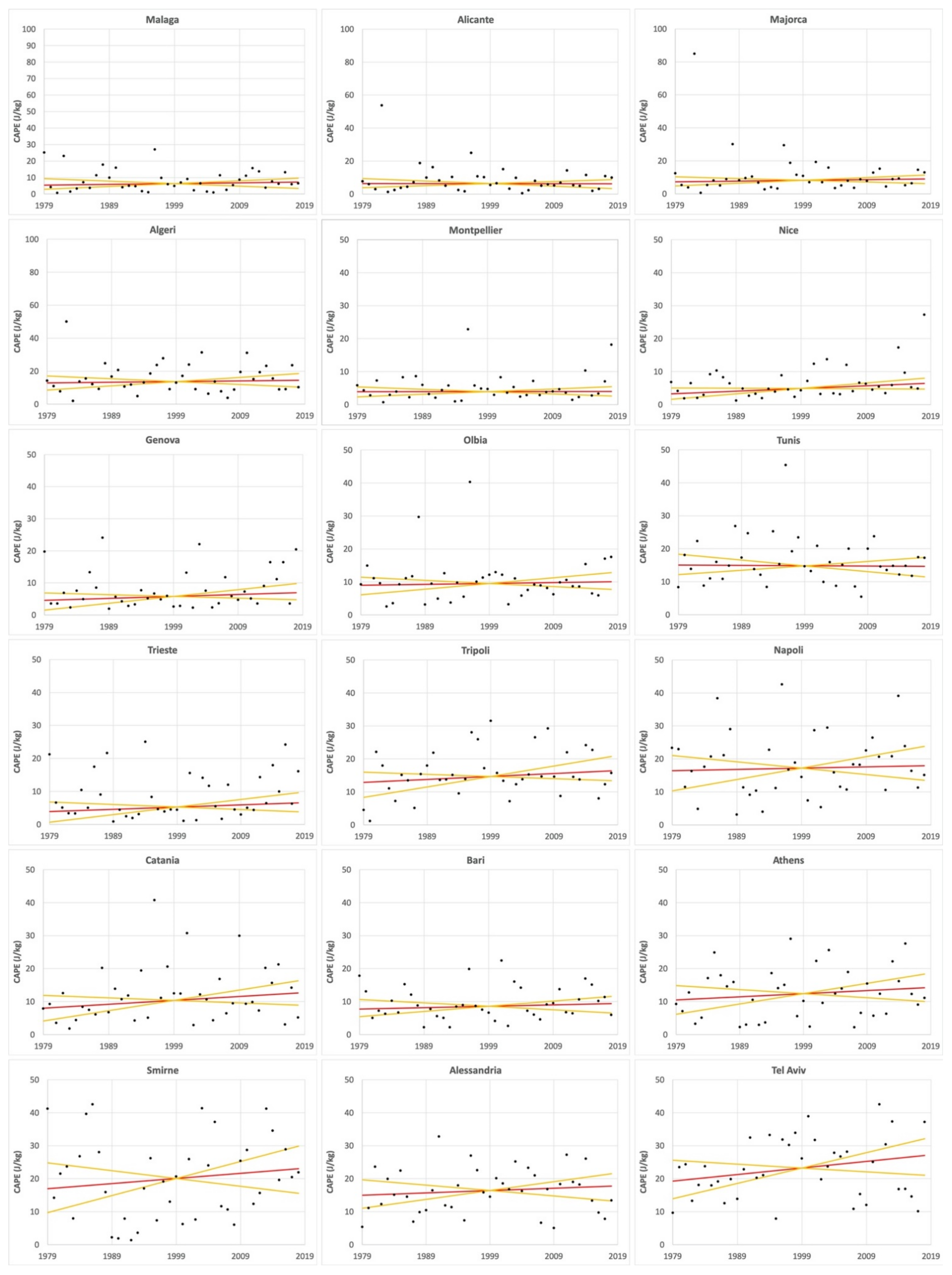
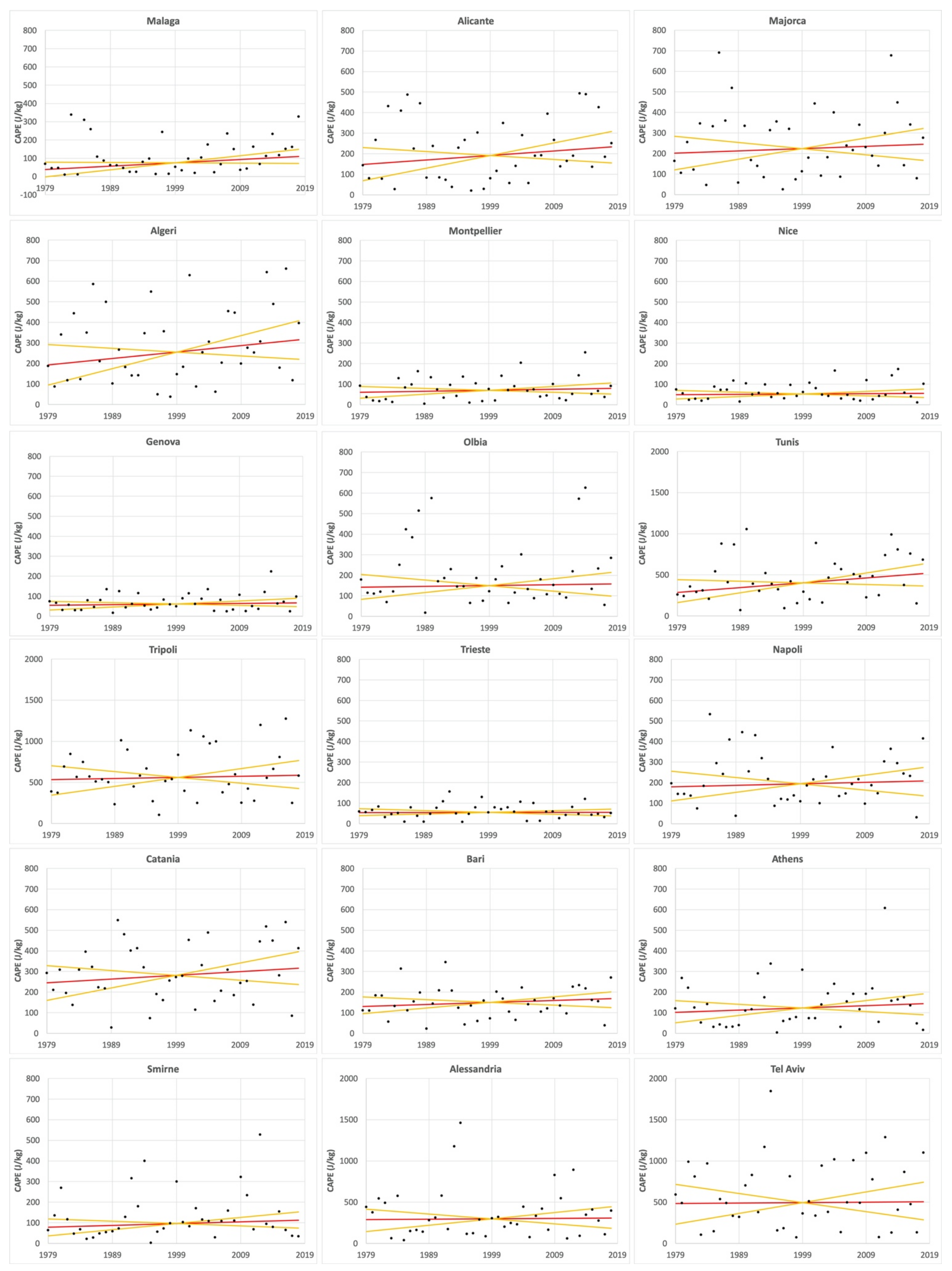
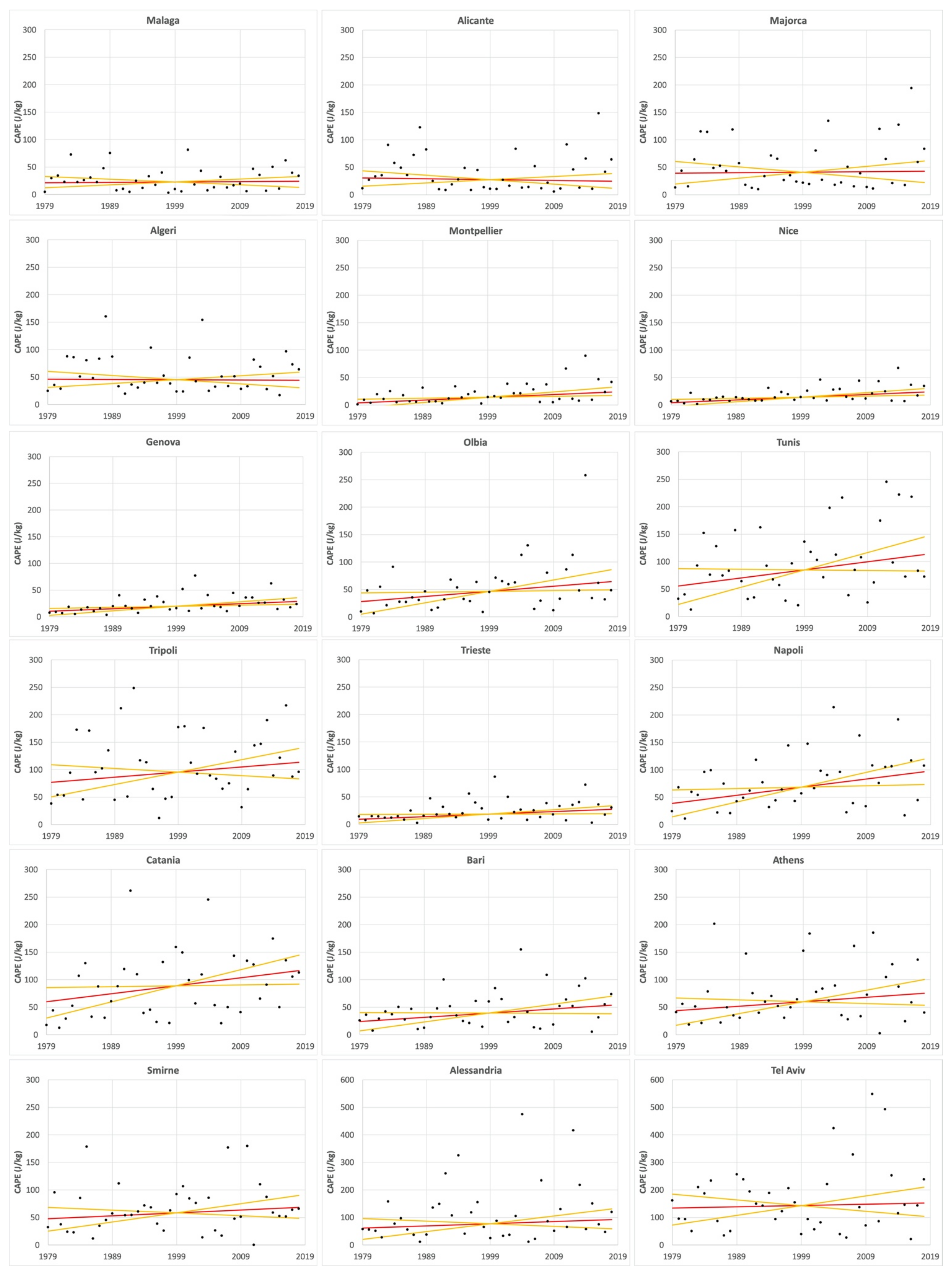
Figure 7, Figure 8 and Figure 9 present annual CAPE mean values for the 1979–2018 period for 100 km2 areas surrounding the 18 major cities facing the Mediterranean Sea in January, October and November; these are the three months when the maximum number of geo-hydrological events happened (Table 1). Sen trend lines and the 95% confidence interval are traced for every graph.
The January series (Figure 7) shows a certain degree of positive trend for Nice, Genova, Olbia, Trieste, Tripoli, Catania, Bari, Athens, Smirne, Alessandria and Tel Aviv. The weak tendencies are not statistically significant according to the results of the Mann–Kendall trend test at 95% significance (Table 3). The low winter season values look quite dispersed over the series, particularly in the Eastern Mediterranean cities. In some cases, the time series was characterized by some particularly high values comparing to the rest of the series: for example, the cities belonging to the Western Mediterranean Sea.
The October series (Figure 8) present considerably higher values typical of the fall season with a more pronounced and widespread positive tendency. Cities facing the Alboran and Balearic seas, the Eastern Mediterranean Sea and those belonging to North Africa, have a positive trend in a quite dispersed series: the high variability is evidenced by the wide confidence interval in Sen tendencies. On the other side, cities facing the northern part of the Mediterranean Sea present less dispersed series. The Mann–Kendall test (Table 3) shows no statistically significant trend.
The November series (Figure 9) shows a positive trend for cities facing the Ligurian Sea, the Tyrrhenian Sea, the Gulf of Gabes, the Adriatic Sea, the Ionian Sea and the Eastern Mediterranean Sea. Such a tendency is confirmed by the Mann–Kendall trend test (Table 3), which shows a statistically significant positive trend for: Montpellier, Nice, Genova, Olbia, Trieste, Napoli and Catania. Besides, the corresponding series present a lower degree of dispersion (Figure 9), while they remain higher for: Tunis, Tripoli, Napoli, Catania, Athens, Smirne, Alessandria and Tel Aviv.
The Mann–Kendall trend test (Table 3) reveals the presence of statistically significant positive trends in other months. In particular, June shows a diffuse increase along almost the whole Mediterranean area, excluding only the far eastern part and the cities of Algeri and Malaga. Significant positive trends were detected in May alongside the cities on the Italian Peninsula and Athens, while August shows trends in cities facing the far Eastern Mediterranean Sea. Some scattered positive trends were detected even in February, March, April, July and September. Considering the whole year, Genova, Trieste and Bari present six months characterized by significant positive trends, followed by Nice, Napoli, Catania and Athens with four months.
The Hurst exponent analysis (Table 4) shows a diffuse presence of persistency in the CAPE series: to differentiate the degree of persistency, values in Table 3 have been highlighted with an orange colour if the Hurst exponent is between 0.650 and 0.849, and in deep orange for values between 0.850 and 1, according to an increasing reliability of the result. The positive persistency appears widespread on almost all the series, both in terms of month and city. The higher values occur in the cities facing the Ligurian, Tyrrhenian and Adriatic seas, with Napoli presenting the highest ones.
3.3. Total Column Water Vapour—TCWV
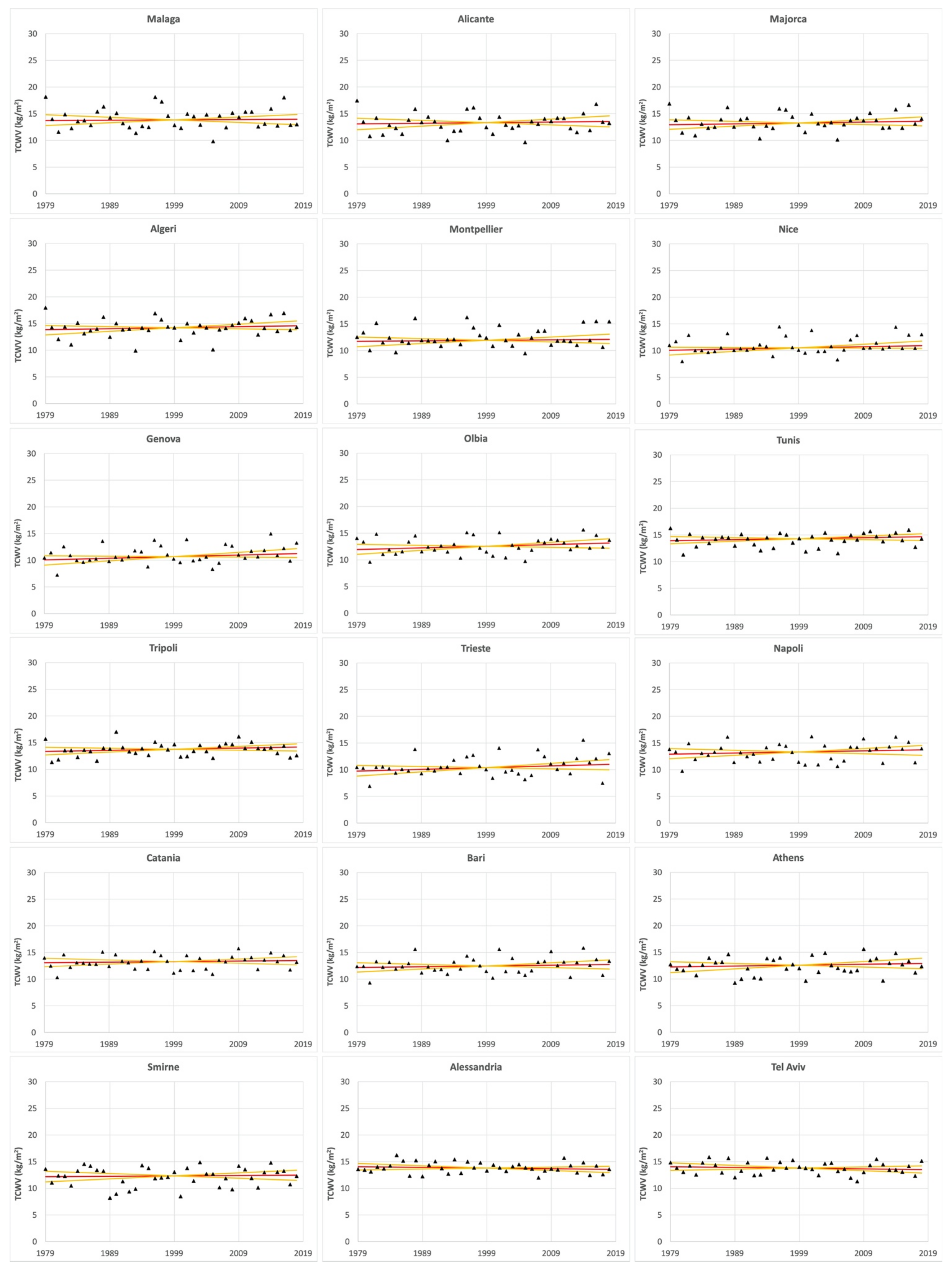
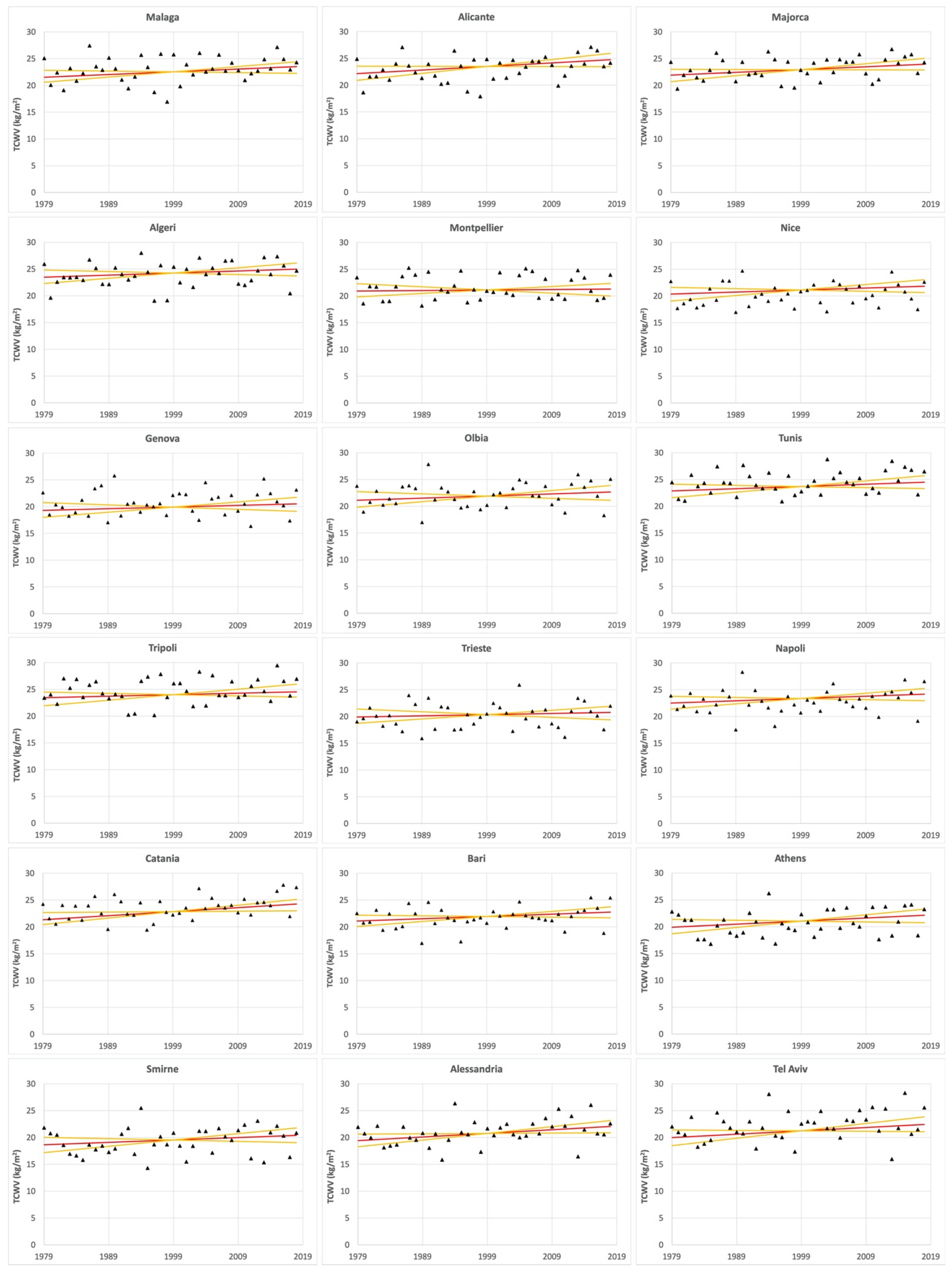
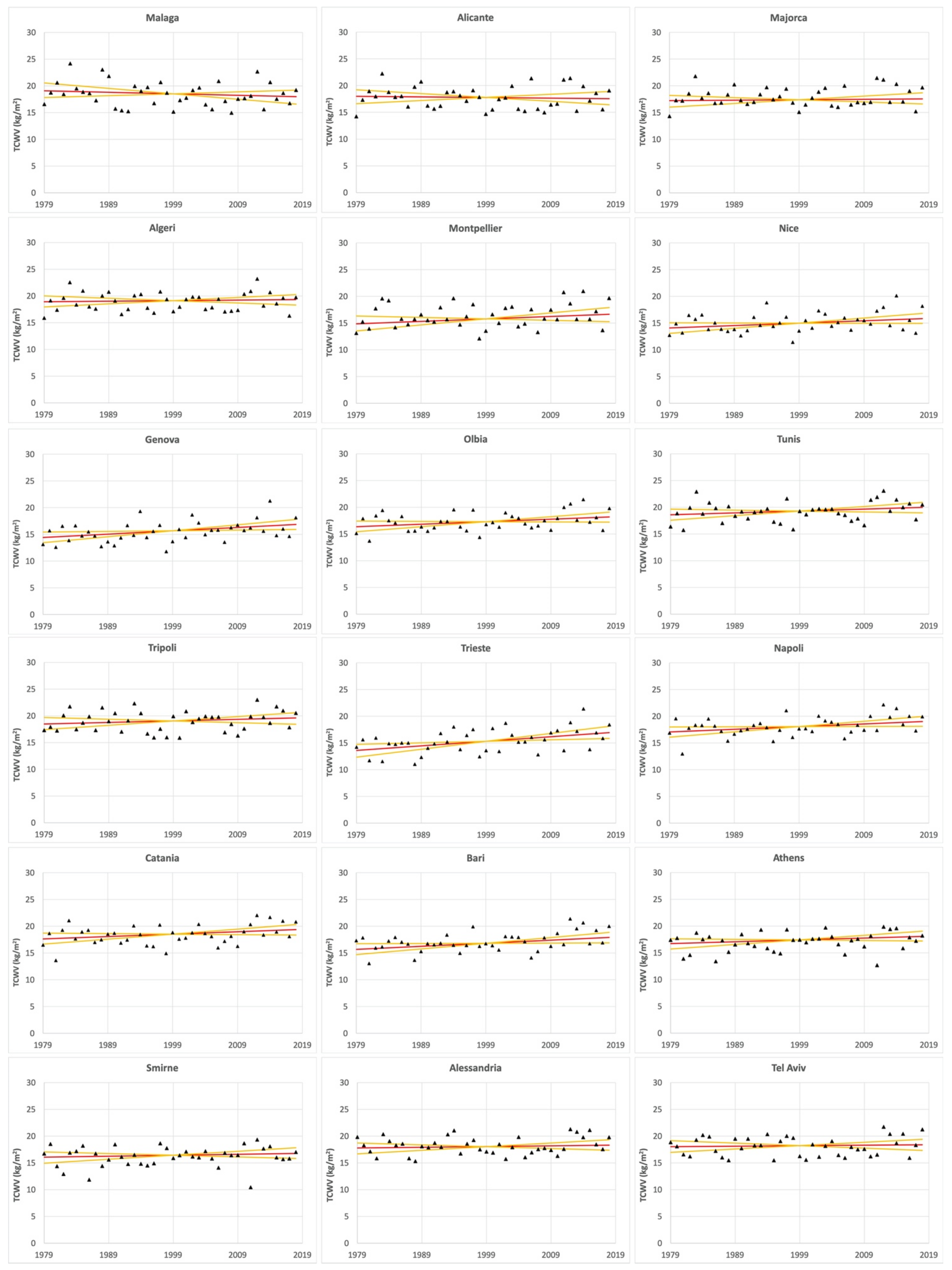
Figure 10, Figure 11 and Figure 12 present the annual TCWV mean values for the 1979–2018 period, over the 100 km2 area surrounding the 18 major cities facing the Mediterranean Sea, in January, October and November respectively. The Sen trend line and the 95% confidence interval are traced for every diagram.
The January data (Figure 10) shows a weak positive trend for Nice, Genova, Olbia, Tunis, Tripoli, Trieste and Napoli. Even in the TCWV data, tendencies are not statistically significant according to the results of the Mann–Kendall trend test at 95% significance (Table 5). Values over the period are less dispersed than those for CAPE values.
The October data (Figure 11) presents a diffused increasing tendency, except for Montpellier. There is a higher degree of dispersion in the period compared to the January values. Areas surrounding Malaga, Alicante, Majorca, Napoli, Catania, Athens, Smirne, Alessandria and Tel Aviv show a major degree of increase. The Mann–Kendall trend test shows a statistically significant positive trend for the Catania and Alessandria series.
The November data (Figure 12) shows an increasing trend for Nice, Genova, Olbia, Trieste, Napoli, Catania, Bari and Athens series. Weakly decreasing trends exist for Malaga and Alicante. Genova, Trieste, Napoli and Bari show a significant increasing trend according to the Mann–Kendall test (Table 5).
The Mann–Kendall trend test (Table 5) reveals a significant increasing trend in April in all the areas surrounding the cities facing the Western Mediterranean Sea, except for Tripoli and Malaga, while in May and June the increase involves the cities facing the Eastern Mediterranean Sea and the Adriatic and Ionian seas. February, July, August and September show increasing values in 2 to 5 cities.
As for CAPE data, the Hurst exponent analysis for TCWV (Table 6) shows a diffuse presence of persistency. The positive persistency appears widespread on almost all the series, both in terms of month and city. The higher Hurst exponent values are concentrated between April and September with more higher values in June.
4. Discussion
The results from the analysis of geo-hydrological events and CAPE and TCWV data trends looks consistent with analyses of precipitation conducted by other authors: the events being the ground effect or consequence of the CAPE and TCWV meteorological instability indicators. Caloiero et al. [46] studied globally gridded precipitation data sets of monthly observations with spatial resolutions of 0.5° longitude/latitude and they found interesting results for the Mediterranean area: yearly results revealed a marked negative rainfall trend in the eastern Mediterranean (more than −20 mm/10 years) and in North Africa (up to −16 mm/10 years), while a relatively large positive trend (more than 20 mm/10 years) occurred in central and northern Europe.
Along similar lines, Hatzianastassiou et al. [47] investigated the precipitation regimes and patterns over the Mediterranean area for the period 1979–2010 using monthly mean satellite data from the Global Precipitation Climatology Project (GPCPv2). They found that while the mean annual precipitation averaged over the study area was 593 ± 203 mm year−1, it exhibited a strong spatial variability ranging from 20 mm year−1 (North Africa) to 1500 mm year−1 (Alps). Furthermore, the early winter and late autumn months (November and December) were the wettest months, with precipitation amounts larger than 60 mm month−1.
Moreover, regarding extreme rainfall events, Benabdelouahab et al. [48] characterized daily rainfall amounts greater than the 95 and 99 quantiles, using the African Rainfall Climatology Version 2 (ARC2, 0.1° × 0.1°, 1983–2020) over north-western Africa and southern Spain, and revealed an annual increase of indicator values of rainfall extreme events, that were still spatial-temporally concentrated. For the other side (eastern Mediterranean) Kostopolou and Jones [49] computed several seasonal and annual climate extreme indices to identify possible changes in temperature- and precipitation-related climate extremes for the period 1958–2000. The western part of the study region, which comprises the central Mediterranean and is represented by Italian stations, showed significant positive trends towards intense rainfall events and greater amounts of precipitation. In contrast, the eastern half showed negative trends in all precipitation indices indicating drier conditions until 2000.
Philandras et al. [50] studied the trends and the variability of annual precipitation totals and annual rain days over land within the Mediterranean region from 40 meteorological stations in the Mediterranean region. They found statistically significant (95% confidence level) negative trends of the annual precipitation totals existed in most Mediterranean regions during the period 1901–2009, with the exception of northern Africa, southern Italy and the western Iberian Peninsula. Interestingly, the annual number of rain days showed a pronounced decrease of 20%, statistically significant (95% confidence level) in representative meteorological stations of the east Mediterranean, while the trends are insignificant for the west and central Mediterranean.
The geo-hydrological events that affected the Mediterranean area between 1979 and 2018, and the trends in CAPE and TCWV mean values for 100 km2 areas, appear coherent: both have been increasing through the entire period over large areas. The statistically significative increases in CAPE and TCWV values show some minor feature differences: spatially and marginally so, even seasonally.
Despite a possibly not perfectly homogeneous and incomplete recording of past geo-hydrological events in the EM-DAT database [51], the differences between the first 20 years and the next 20 is strong and is about four times greater (Figure 4). Besides, the monthly data (Table 1) show how, starting from around the year 2000, events occurred in every season and even more than once per month. Further, the increase in numbers of events, which appears to have progressively accelerated in the early three decades, is shared by the majority of sub-types events (Figure 3). The lack of increase in landslides count may be explained by the event type: diffuse small shallow landslides were not included in the database. In fact, it contains only large events that caused extensive damage and even casualties. Including rain-triggered shallow landslides could change this result, as their incidence has been frequent in some areas as testified by many authors [52,53,54,55,56,57,58,59,60,61] but obtaining homogeneous and precise data for the whole Mediterranean area for the whole period is quite difficult.
Southern Mediterranean Sea countries have been subjected to some large scale and high impact events, while the northern Mediterranean countries have been subjected to a higher number of events, each causing fewer casualties. This disparity could be partially due to some event differences: on one hand, the large floods of the River Nile in November 1994, the large storm that hit the Moroccan Atlas Mountains in August 1995 [62] coupled to geomorphic predisposing conditions, the cyclonic storm in November 2001 that hit Algeria and, on the other, several more localized events hitting the European countries [63,64,65,66]. Notwithstanding this, land use and vulnerability conditions have probably played an important role in this differentiation between the North African countries and the European ones. Large European territories suffer for a high percentage of soil sealing and for the lack of proper risk mitigation measures [67,68,69,70,71], which influence the impact of severe events. Nevertheless, the different economic conditions of north African territories cause a further planning inadequacy [72,73] for land usage, exposing them to a high geo-hydrologic risk.
Most of the recorded events happened in January, November, October, and December. Throughout these months, the CAPE and TCWV time data series showed increasing trends (Table 7, Table 8 and Table 9), although only in some cases with statistical significance. In January and December, the lack of a Mann–Kendall statistically significant trend for CAPE and TCWV values is accompanied by quite widespread persistence marks, as evidenced by the high values for the Hurst exponent in areas often hit by geo-hydrological events: Genova, Nice and Catania for CAPE values both in January and December. Besides, persistence characterizes most of the CAPE series in December. Further, in November, when many highly damaging events happened diffusively along the western and southern Italian coastlines and the French Riviera, the CAPE series showed statically significant positive trends in Montpellier, Nice, Genova, Olbia, Trieste, Napoli, and Catania. Strong persistence is present in the same series and more diffusively in others in the Western Mediterranean area. Similar features are recorded by the TCWV series, but for a more limited series: Genova, Trieste, Napoli, and Bari. In October, persistence was recorded in only some series. In summary, in January (Table 7) statistically insignificant trends in the CAPE values are present for the central and eastern Mediterranean, with many series being quite dispersed and, in some cases, accompanied by persistency. The same behaviour appears for the TCWV values but limited to the central Mediterranean. In October (Table 8), the increasing trend in the CAPE values is limited to the western Mediterranean and is still not statistically significant, while the TCWV data looks to be increasing all over the studied cities with some significant and persistence features. November (Table 9) shows the highest degree of concordance between the trend in CAPE and TCWV values: the central Mediterranean cities appear to be affected by increasing significant trends and persistence features.
This behaviour may be interpreted as a tendency for geo-hydrological intense events predisposing factors, as suggested by other researchers [74]. In fact, the high intensity precipitative phenomena are mostly linked to the contrast between the warm sea surface and cold air masses coming from outside the Mediterranean, which usually happens in October and November. The detected trends could suggest the extension of these conditions to December and January, as a possible consequence of increasing sea surface temperatures, whose trend has been documented by many researchers [75,76,77,78,79]. Besides, these features are consistent with the increasing extreme precipitations evidenced by other authors [49,50].
Considering the geo-hydrological events grouped by decade (Table 10), increasing numbers of events occurred in the French Mediterranean area from September through December after the year 2000 (Table 10), as recorded in the EM–DAT database: the increasing numbers of events are coherent with the trend in CAPE values in November (Table 9), and the associated persistency that extends to the Ligurian Sea coastline. Again, in November, the increasing trends in CAPE values for cities belonging to the southern Tyrrhenian Sea and to the Ionian Sea are consistent with the high numbers of events (11) registered for south Italy (Table 10), with an increasing frequency starting from the year 2000.
In the Balkan area, event occurrence is quite evenly distributed over the year, but it is higher between November and February, and the increase has been substantial since the year 2000 (Table 10). Besides, it must be noted that no event is present in the database before the year 1999 for that area, suggesting a possible lack in the database.
Considering the Eastern Mediterranean area, the highest incidence in Greece is between October and November, in Turkey between May and August, and in the coastal Middle East countries, between December and February (Table 10). The event increase in all these areas, during the study period, is quite evident. Regarding the far eastern area, the trends in TCWV values, the series persistence and the CAPE series persistence are consistent with the increase in numbers of geo-hydrological events for Smirne in summer; for the rest of studied Middle East cities, the increasing numbers of events occurring in January and February seems not related to CAPE nor to TCWV trends or persistence.
The Western area, including Spain, Portugal, Morocco, Algeria and Tunisia is characterized by a substantial increase in number of events, between the first two decades and the second two (Table 10); the maximum number is in fall and early winter. This trend is consistent with the CAPE series persistence from September through December.
Finally, the CAPE and TCWV data analyses were limited to the monthly mean values for the 100 km2 surrounding 18 major cities facing the Mediterranean. Despite this limitation, in both cases trends were detected and are consistent with the increase in the number of the geo-hydrologic events. Moreover, the CAPE data is an indicator of atmospheric instability and then linked to extreme events, while the TCWV data is related to the availability of precipitable water. A further step of the research will focus on other spatialized variables, allowing a more in-depth search for the correlation with the geo-hydrologic events.
5. Conclusions
This work presents an innovative approach to identify potential relationships between the trends in the occurrence of geo-hydrologic events that impacted the Mediterranean area between 1979 and 2018 (EM–DAT source) and some meteorological indices (CAPE and TCWV) that are predictors of severe weather conditions. The possible presence of trends or tendencies is detected by using the Mann–Kendall test, the Sen’s slope estimator and the Hurst exponent. In the first part of the work, the geo-hydrological severe events that occurred in the countries facing or close to the Mediterranean area, for the 40 years period 1978–2018, were analysed, and it was concluded that events in the last two decades are about four times the number of those in 1979–1988, and more than two times the number of those in 1989–1998. Conversely, no trend emerges over the 40 years period in terms of number of fatalities. When focusing on the distribution of sub-type events by year, between 1979 and 2018, the study clearly shows an increase in number of riverine and flash floods, and of extra-tropical and convective storms from the year 2000, in contrast to their lower incidence in the previous periods, with an even stronger signal in the last decade 2009–2018. Subsequently, the study focused on the analysis of CAPE and TCWV data for 18 major cities facing the Mediterranean Sea, and it allowed the detection of interesting trends in different cities even while varying geographically and seasonally, but still with higher values in fall months. Future work will be devoted to a spatial analysis at the entire Mediterranean region scale of the aforementioned trends by including additional meteorological indices (e.g., microphysics oriented).
Author Contributions
Conceptualization, G.P. and A.P.; methodology, G.P. and A.P.; software, G.P.; validation, G.P. and A.P.; formal analysis, G.P.; investigation, G.P.; data curation, G.P.; writing—original draft preparation, G.P. and A.P.; writing—review and editing, G.P. and A.P.; visualization, G.P.; supervision, G.P. and A.P.; funding acquisition, G.P. and A.P. All authors have read and agreed to the published version of the manuscript.
Funding
This research received no external funding.
Conflicts of Interest
The authors declare no conflict of interest.
References
- Drobinski, P.; Ducrocq, V.; Alpert, P.; Anagnostou, E.; Béranger, K.; Borga, M.; Braud, I.; Chanzy, A.; Davolio, S.; Delrieu, G.; et al. HyMeX: A 10-Year Multidisciplinary Program on the Mediterranean Water Cycle. Bull. Am. Meteorol. Soc. 2014, 95, 1063–1082. [Google Scholar] [CrossRef]
- Mariotti, A.; Struglia, M.V.; Zeng, N.; Lau, K.M. The hydrological cycle in the Mediterranean region and implications for the water budget of the Mediterranean Sea. J. Clim. 2002, 15, 1674–1690. [Google Scholar] [CrossRef] [Green Version]
- Thornes, J.; López-Bermúdez, F.; Woodward, J. Hydrology, River Regimes, and Sediment Yield. In The Physical Geography of the Mediterranean; Woodward, J., Ed.; Oxford University Press: Oxford, UK, 2009; pp. 229–253. [Google Scholar]
- Madakumbura, G.D.; Kim, H.; Utsumi, N.; Shiogama, H.; Fischer, E.M.; Seland, Ø.; Scinocca, J.F.; Mitchell, D.M.; Hirabayashi, Y.; Oki, T. Event-to-event intensification of the hydrologic cycle from 1.5 °C to a 2 °C warmer world. Sci. Rep. 2019, 9, 1–7. [Google Scholar] [CrossRef]
- Petrucci, O.; Papagiannaki, K.; Aceto, L.; Boissier, L.; Kotroni, V.; Grimalt, M.; Llasat, M.C.; Llasat-Botija, M.; Rosselló, J.; Pasqua, A.A.; et al. MEFF: The database of MEditerranean Flood Fatalities (1980 to 2015). J. Flood Risk Manag. 2019, 12, e12461. [Google Scholar] [CrossRef] [Green Version]
- Giorgi, F. Climate Change Hot-Spots. Geophys. Res. Lett. 2006, 33, L08707. [Google Scholar] [CrossRef]
- Llasat, M.C.; Llasat-Botija, M.; Prat, M.A.; Porcu, F.; Price, C.; Mugnai, A.; Lagouvardos, K.; Kotroni, V.; Katsanos, D.; Michaelides, S.; et al. High-impact floods and flash floods in Mediterranean countries: The FLASH preliminary database. Adv. Geosci. 2010, 23, 47–55. [Google Scholar] [CrossRef] [Green Version]
- Vinet, F.; Bigot, V.; Petrucci, O.; Papagiannaki, K.; Llasat, M.C.; Kotroni, V.; Boissier, L.; Aceto, L.; Grimalt, M.; Llasat-Botija, M.; et al. Mapping Flood-Related Mortality in the Mediterranean Basin. Results from the MEFF v2.0 DB. Water 2019, 11, 2196. [Google Scholar] [CrossRef] [Green Version]
- Reale, O.; Feudale, L.; Turato, B. Evaporative moisture sources during a sequence of floods in the Mediterranean region. Geophys. Res. Lett. 2001, 28, 2085–2088. [Google Scholar] [CrossRef]
- Molini, L.; Parodi, A.; Rebora, N.; Craig, G. Classifying severe rainfall events over Italy by hydrometeorological and dynamical criteria. Q. J. R. Meteorol. Soc. 2011, 137, 148–154. [Google Scholar] [CrossRef]
- Pinto, J.G.; Ulbrich, S.; Parodi, A.; Rudari, R.; Boni, G.; Ulbrich, U. Identification and ranking of extraordinary rainfall events over Northwest Italy: The role of Atlantic moisture. J. Geophys. Res. Atmos. 2013, 118, 2085–2097. [Google Scholar] [CrossRef] [Green Version]
- Grazzini, F.; Fragkoulidis, G.; Teubler, F.; Wirth, V.; Craig, G.C. Extreme precipitation events over northern Italy. Part II: Dynamical precursors. Q. J. R. Meteorol. Soc. 2021, 147, 1237–1257. [Google Scholar] [CrossRef]
- Bevis, M.; Businger, S.; Herring, T.A.; Rocken, C.; Anthes, R.A.; Ware, R.H. GPS meteorology: Remote sensing of atmospheric water vapor using the Global Positioning System. J. Geophys. Res. Atmos. 1992, 97, 15787–15801. [Google Scholar] [CrossRef]
- Poletti, M.L.; Parodi, A.; Turato, B. Severe hydrometeorological events in Liguria region: Calibration and validation of a meteorological indices-based forecasting operational tool. Meteorol. Appl. 2017, 24, 560–570. [Google Scholar] [CrossRef] [Green Version]
- Rohling, E.J.; Abu-Zied, R.H.; Casford, J.S.L.; Hayes, A.; Hoogakker, B.A.A. The marine environment: Present and past. In The Physical Geography of the Mediterranean; Jamie, W., Ed.; Oxford University Press: Oxford, UK, 2009; pp. 33–67. [Google Scholar]
- Mather, A.E. Tectonic setting and landscape development. In The Physical Geography of the Mediterranean; Jamie, W., Ed.; Oxford University Press: Oxford, UK, 2009; pp. 5–32. [Google Scholar]
- Llasat, M.C. High magnitude storms and floods. In The Physical Geography of the Mediterranean; Jamie, W., Ed.; Oxford University Press: Oxford, UK, 2009; pp. 513–540. [Google Scholar]
- Harding, A.E.; Palutikof, J.; Holt, T. The climate system. In The Physical Geography of the Mediterranean; Jamie, W., Ed.; Oxford University Press: Oxford, UK, 2009; pp. 69–88. [Google Scholar]
- Koppen, W. Das geographische system der klimat. In Handbuch der Klimatologie; Gebruder Borntraeger: Stuttgart, Germany, 1936; Volume 46, Available online: http://koeppen-geiger.vu-wien.ac.at/pdf/Koppen_1936.pdf (accessed on 19 December 2021).
- Gil, V.E.; Genovés, A.; Picornell, M.A.; Jansa, A. Automated database of cyclones from the ECMWF model: Preliminary comparison between west and east Mediterranean basins. In Proceedings of the 4th EGS Plinius Conference, Mallorca, Spain, 2–4 October 2002; Universitat de les Illes Baleares: Palma, Spain, 2003. [Google Scholar]
- Paliaga, G.; Donadio, C.; Bernardi, M.; Faccini, F. High-Resolution Lightning Detection and Possible Relationship with Rainfall Events over the Central Mediterranean Area. Remote Sens. 2019, 11, 1601. [Google Scholar] [CrossRef] [Green Version]
- Estrela, T.; Marcuello, C.; Dimas, M. Las Aguas Continentales en Los Países Mediterráneos de la Unión Europea; Report of the CEDEX; Ministerio de Fomento: Madrid, Spain, 2000. [Google Scholar]
- Faccini, F.; Luino, F.; Paliaga, G.; Roccati, A.; Turconi, L. Flash Flood Events along the West Mediterranean Coasts: Inundations of Urbanized Areas Conditioned by Anthropic Impacts. Land 2021, 10, 620. [Google Scholar] [CrossRef]
- EM-DAT, CRED/UCLouvain, Brussels, Belgium. Available online: www.emdat.be (accessed on 20 August 2020).
- Hersbach, H.; Bell, B.; Berrisford, P.; Biavati, G.; Horányi, A.; Muñoz Sabater, J.; Nicolas, J.; Peubey, C.; Radu, R.; Rozum, I.; et al. ERA5 Monthly Averaged Data on Single Levels from 1979 to Present. Available online: https://cds.climate.copernicus.eu/cdsapp#!/dataset/reanalysis-era5-single-levels-monthly-means?tab=overview (accessed on 6 June 2020).
- Real Statistics with Excel. Available online: https://www.real-statistics.com (accessed on 29 August 2021).
- Kendall, M.G.; Gibbons, J.D. Rank Correlation Methods, 5th ed.; Griffin: London, UK, 1990. [Google Scholar]
- Hamed, K.H. Exact distribution of the Mann-Kendall trend test statistic for persistent data. J. Hydrol. 2009, 365, 86–94. [Google Scholar] [CrossRef]
- Douglas, E.M.; Vogel, R.M.; Kroll, C.N. Trends in floods and low flows in the United States: Impact of spatial correlation. J. Hydrol. 2000, 240, 90–105. [Google Scholar] [CrossRef]
- Tabari, H.; Shifteh Somee, B.; Rezaeian Zadeh, M. Testing for long-term trends in climatic variables in Iran. Atmos. Res. 2011, 100, 132–140. [Google Scholar] [CrossRef]
- Gocic, M.; Slavisa, T. Analysis of changes in meteorological variables using Mann-Kendall and Sen’s slope estimator statistical tests in Serbia. Glob. Planet. Chang. 2013, 100, 172–182. [Google Scholar] [CrossRef]
- Shi, P.; Wu, M.; Qu, S.; Jiang, P.; Qiao, X.; Chen, X.; Zhou, M.; Zhang, Z. Spatial distribution and temporal trends in precipitation concentration indices for the Southwest China. Water Resour. Manag. 2015, 29, 3941–3955. [Google Scholar] [CrossRef]
- Sen, P.K. Estimates of the regression coefficient based on Kendall’s tau. J. Am. Stat. Assoc. 1968, 63, 1379–1389. [Google Scholar] [CrossRef]
- Einstein, A. Investigations on the Theory of Brownian Movement; Dover Inc.: New York, NY, USA, 1956. [Google Scholar]
- Granero, M.S.; Segovia, J.T.; Pérez, J.G. Some comments on Hurst exponent and the long memory processes on capital markets. Phys. A Stat. Mech. Appl. 2008, 387, 5543–5551. [Google Scholar] [CrossRef]
- Hurst, H.E. Long-term storage capacity of reservoirs. Tran. Am. Soc. Civ. Eng. 1951, 116, 770–799. [Google Scholar] [CrossRef]
- Hamed, K.H. Improved finite-sample Hurst exponent estimates using rescaled range analysis. Water Resour. Res. 2007, 43, 413. [Google Scholar] [CrossRef]
- Xu, J.H.; Chen, Y.N.; Li, W.H.; Dong, S. Long-term trend and fractal of annual runoff process in mainstream of Tarim river. Chin. Geogr. Sci. 2008, 18, 77–84. [Google Scholar] [CrossRef] [Green Version]
- Huang, J.; Sun, S.; Zhang, J. Detection of trends in precipitation during 1960–2008 in Jiangxi province, southeast China. Theor. Appl. Climatol. 2013, 114, 237–251. [Google Scholar] [CrossRef]
- Benavides-Bravo, F.G.; Martinez-Peon, D.; Benavides-Ríos, Á.G.; Walle-García, O.; Soto-Villalobos, R.; Aguirre-López, M.A. A Climate-Mathematical Clustering of Rainfall Stations in the Río Bravo-San Juan Basin (Mexico) by Using the Higuchi Fractal Dimension and the Hurst Exponent. Mathematics 2021, 9, 2656. [Google Scholar] [CrossRef]
- Xu, Z.; Tang, Y.; Connor, T.; Li, D.; Li, Y.; Liu, J. Climate variability and trends at a national scale. Sci. Rep. 2017, 7, 1–10. [Google Scholar] [CrossRef] [PubMed]
- López-Lambraño, A.A.; Fuentes, C.; López-Ramos, A.A.; Mata-Ramírez, J.; López-Lambraño, M. Spatial and temporal Hurst exponent variability of rainfall series based on the climatological distribution in a semiarid region in Mexico. Atmósfera 2018, 31, 199–219. [Google Scholar] [CrossRef]
- Mandelbrot, B.B.; Wallis, J.R. Robustness of the rescaled range R/S in the measurement of noncyclic long run statistical dependence. Water Resour. Res. 1969, 5, 967–988. [Google Scholar] [CrossRef]
- Klemeš, V.; Srikanthan, R.; McMahon, T.A. Long-memory flow models in reservoir analysis: What is their practical value? Water Resour. Res. 1981, 17, 737–751. [Google Scholar] [CrossRef]
- Mandelbrot, B. When can price be arbitrage deficiently? A limit to the validity of the random walk and martingale models. Rev. Econ. Stat. 1971, 53, 225–236. [Google Scholar] [CrossRef]
- Caloiero, T.; Coscarelli, R.; Ferrari, E.; Mancini, M. Precipitation changes in Southern Italy linked to global scale oscillation indexes. Nat. Hazards Earth Syst. Sci. 2011, 11, 1683–1694. [Google Scholar] [CrossRef]
- Hatzianastassiou, N.; Papadimas, C.D.; Lolis, C.J.; Bartzokas, A.; Levizzani, V.; Pnevmatikos, J.D.; Katsoulis, B.D. Spatial and temporal variability of precipitation over the Mediterranean Basin based on 32-year satellite Global Precipitation Climatology Project data, part I: Evaluation and climatological patterns. Int. J. Climatol. 2016, 36, 4741–4754. [Google Scholar] [CrossRef]
- Benabdelouahab, T.; Gadouali, F.; Boudhar, A.; Lebrini, Y.; Hadria, R.; Salhi, A. Analysis and trends of rainfall amounts and extreme events in the Western Mediterranean region. Theor. Appl. Climatol. 2020, 141, 309–320. [Google Scholar] [CrossRef]
- Kostopoulou, E.; Jones, P.D. Assessment of climate extremes in the Eastern Mediterranean. Meteorol. Atmos. Phys. 2005, 89, 69–85. [Google Scholar] [CrossRef]
- Philandras, C.M.; Nastos, P.T.; Kapsomenakis, J.; Douvis, K.C.; Tselioudis, G.; Zerefos, C.S. Long term precipitation trends and variability within the Mediterranean region. Nat. Hazards Earth Syst. Sci. 2011, 11, 3235–3250. [Google Scholar] [CrossRef] [Green Version]
- Pereira, S.; Diakakis, M.; Deligiannakis, G.; Zêzere, J.L. Comparing flood mortality in Portugal and Greece (Western and Eastern Mediterranean). Int. J. Disaster Risk Reduct. 2017, 22, 147–157. [Google Scholar] [CrossRef]
- Cascini, L.; Cuomo, S.; Della Sala, M. Spatial and temporal occurrence of rainfall-induced shallow landslides of flow type: A case of Sarno-Quindici, Italy. Geomorphology 2011, 126, 148–158. [Google Scholar] [CrossRef]
- Saidi, M.E.M.; Boukrim, S.; Fniguire, F.; Ramromi, A. Les écoulements superficiels sur le Haut Atlas de Marrakech cas des débits extrêmes. Larhyss J. 2012, 10, 75–90. [Google Scholar]
- Brandolini, P.; Cevasco, A.; Capolongo, D.; Pepe, G.; Lovergine, F.; Del Monte, M. Response of Terraced Slopes to a Very Intense Rainfall Event and Relationships with Land Abandonment: A Case Study from Cinque Terre (Italy). Land Degrad. Dev. 2018, 29, 630–642. [Google Scholar] [CrossRef]
- Valenzuela, P.; Iglesias, M.; Domínguez-Cuesta, M.J.; García, M.A.M. Meteorological Patterns Linked to Landslide Triggering in Asturias (NW Spain): A Preliminary Analysis. Geosciences 2018, 8, 18. [Google Scholar] [CrossRef] [Green Version]
- Fusco, F.; De Vita, P.; Mirus, B.B.; Baum, R.L.; Allocca, V.; Tufano, R.; Di Clemente, E.; Calcaterra, D. Physically Based Estimation of Rainfall Thresholds Triggering Shallow Landslides in Volcanic Slopes of Southern Italy. Water 2019, 11, 1915. [Google Scholar] [CrossRef] [Green Version]
- Luino, F.; De Graff, J.; Roccati, A.; Biddoccu, M.; Cirio, C.G.; Faccini, F.; Turconi, L. Eighty Years of Data Collected for the Determination of Rainfall Threshold Triggering Shallow Landslides and Mud-Debris Flows in the Alps. Water 2019, 12, 133. [Google Scholar] [CrossRef] [Green Version]
- Roccati, A.; Paliaga, G.; Luino, F.; Faccini, F.; Turconi, L. Rainfall Threshold for Shallow Landslides Initiation and Analysis of Long-Term Rainfall Trends in a Mediterranean Area. Atmosphere 2020, 11, 1367. [Google Scholar] [CrossRef]
- Jordanova, G.; Gariano, S.L.; Melillo, M.; Peruccacci, S.; Brunetti, M.T.; Auflič, M.J.J. Determination of Empirical Rainfall Thresholds for Shallow Landslides in Slovenia Using an Automatic Tool. Water 2020, 12, 1449. [Google Scholar] [CrossRef]
- Fernández, T.; Pérez-García, J.; Gómez-López, J.; Cardenal, J.; Moya, F.; Delgado, J. Multitemporal Landslide Inventory and Activity Analysis by Means of Aerial Photogrammetry and LiDAR Techniques in an Area of Southern Spain. Remote Sens. 2021, 13, 2110. [Google Scholar] [CrossRef]
- Lainas, S.; Depountis, N.; Sabatakakis, N. Preliminary Forecasting of Rainfall-Induced Shallow Landslides in the Wildfire Burned Areas of Western Greece. Land 2021, 10, 877. [Google Scholar] [CrossRef]
- Saouabe, T.; El Khalki, E.M.; Saidi, M.E.M.; Najmi, A.; Hadri, A.; Rachidi, S.; Jadoud, M.; Tramblay, Y. Evaluation of the GPM-IMERG Precipitation Product for Flood Modeling in a Semi-Arid Mountainous Basin in Morocco. Water 2020, 12, 2516. [Google Scholar] [CrossRef]
- Diakakis, M.; Mavroulis, S.D.; Deligiannakis, G. Floods in Greece, a statistical and spatial approach. Nat. Hazards 2012, 62, 485–500. [Google Scholar] [CrossRef]
- Rebora, N.; Molini, L.; Casella, E.; Comellas, A.; Fiori, E.; Pignone, F.; Siccardi, F.; Silvestro, F.; Tanelli, S.; Parodi, A. Extreme Rainfall in the Mediterranean: What Can We Learn from Observations? J. Hydrometeorol. 2013, 14, 906–922. [Google Scholar] [CrossRef]
- Barrera-Escoda, A.; Llasat, M.C. Evolving flood patterns in a Mediterranean region (1301–2012) and climatic factors–the case of Catalonia. Hydrol. Earth Syst. Sci. 2015, 19, 465–483. [Google Scholar] [CrossRef] [Green Version]
- Faccini, F.; Paliaga, G.; Piana, P.; Sacchini, A.; Watkins, C. The Bisagno stream catchment (Genoa, Italy) and its major floods: Geomorphic and land use variations in the last three centuries. Geomorphology 2016, 273, 14–27. [Google Scholar] [CrossRef]
- Paliaga, G.; Luino, F.; Turconi, L.; Marincioni, F.; Faccini, F. Exposure to Geo-Hydrological Hazards of the Metropolitan Area of Genoa, Italy: A Multi-Temporal Analysis of the Bisagno Stream. Sustainability 2020, 12, 1114. [Google Scholar] [CrossRef] [Green Version]
- Kaspersen, P.S.; Ravn, N.H.; Arnbjerg-Nielsen, K.; Madsen, H.; Drews, M. Comparison of the impacts of urban development and climate change on exposing European cities to pluvial flooding. Hydrol. Earth Syst. Sci. 2017, 21, 4131–4147. [Google Scholar] [CrossRef] [Green Version]
- Acquaotta, F.; Faccini, F.; Fratianni, S.; Paliaga, G.; Sacchini, A.; Viliìmek, V. Increased flash flooding in Genoa Metropolitan Area: A combination of climate changes and soil consumption? Meteorol. Atmos. Phys. 2019, 131, 1–12. [Google Scholar] [CrossRef]
- Luino, F.; Paliaga, G.; Roccati, A.; Sacchini, A.; Turconi, L.; Faccini, F. Anthropogenic changes in the alluvial plains of the Tyrrhenian Ligurian basins. Rend. Online Soc. Geol. Ital. 2019, 48, 10–16. [Google Scholar] [CrossRef]
- Paliaga, G.; Faccini, F.; Luino, F.; Roccati, A.; Turconi, L. A clustering classification of catchment anthropogenic modification and relationships with floods. Sci. Total Environ. 2020, 740, 139915. [Google Scholar] [CrossRef]
- Loudyi, D.; Kantoush, S.A. Flood risk management in the Middle East and North Africa (MENA) region. Urban Water J. 2020, 17, 379–380. [Google Scholar] [CrossRef]
- Hamlat, A.; Kadri, C.B.; Guidoum, A.; Bekkaye, H. Flood hazard areas assessment at a regional scale in M’zi wadi basin, Algeria. J. Afr. Earth Sci. 2021, 182, 104281. [Google Scholar] [CrossRef]
- Kelebek, M.; Batibeniz, F.; Önol, B. Exposure Assessment of Climate Extremes over the Europe–Mediterranean Region. Atmosphere 2021, 12, 633. [Google Scholar] [CrossRef]
- Pastor, F.; Valiente, J.A.; Palau, J.L. Sea Surface Temperature in the Mediterranean: Trends and Spatial Patterns (1982–2016). Pure Appl. Geophys. 2017, 175, 4017–4029. [Google Scholar] [CrossRef] [Green Version]
- Shaltout, M.; Omstedt, A. Recent sea surface temperature trends and future scenarios for the Mediterranean Sea. Oceanologia 2014, 56, 411–443. [Google Scholar] [CrossRef] [Green Version]
- Pisano, A.; Marullo, S.; Artale, V.; Falcini, F.; Yang, C.; Leonelli, F.E.; Santoleri, R.; Nardelli, B.B. New Evidence of Mediterranean Climate Change and Variability from Sea Surface Temperature Observations. Remote Sens. 2020, 12, 132. [Google Scholar] [CrossRef] [Green Version]
- Pastor, F.; Valiente, J.A.; Khodayar, S. A warming Mediterranean: 38 years of increasing sea surface temperature. Remote Sens. 2020, 12, 2687. [Google Scholar] [CrossRef]
- Stathopoulos, C.; Patlakas, P.; Tsalis, C.; Kallos, G. The Role of Sea Surface Temperature Forcing in the Life-Cycle of Mediter-ranean Cyclones. Remote Sens. 2020, 12, 825. [Google Scholar] [CrossRef] [Green Version]
Figure 1.
The Mediterranean area and the main cities facing the sea where the trends in CAPE and TCWV data were investigated in a 100 km2 cell. The names of the examined countries are highlighted in light blue: ALB: Albania; AUT: Austria; BIH: Bosnia and Herzegovina; CHE: Switzerland; CYP: Cyprus; DZA: Algeria; EGY: Egypt; ESP: Spain; FRA: France; GRC: Greece; HRV: Croatia; ISR: Israel; ITA: Italy; JOR: Jordan; LBN: Lebanon; LBY: Libya; MAR: Morocco; MKD: Macedonia; MNE: Montenegro; PRT: Portugal; PSE: Palestine; SCG: Serbia Montenegro; SRB: Serbia; SVN: Slovenia; SYR: Syria; TUN: Tunisia; TUR: Turkey; YUG: Yugoslavia.

Figure 2.
The investigated area with countries grouped by number of severe geo-hydrological events in the period 1979–2018. As a single event often produced several ground effects, these ones are highlighted with yellow dots. Some of them are superimposed due to the spatial scale, or to imprecise geolocation i.e., in Corsica (FRA), while in many cases, one event impacted several contiguous areas.

Figure 3.
The schematic diagram of CAPE and TCWV analysis.

Figure 4.
The number of geo-hydrological events and related casualties, collected from the EM–DAT database for the period 1979–2018 for the examined countries, per year (left) and per decade (right).
Figure 4.
The number of geo-hydrological events and related casualties, collected from the EM–DAT database for the period 1979–2018 for the examined countries, per year (left) and per decade (right).

Figure 5.
The number of events by sub-type per year.

Figure 6.
The decadal economic loss (EM-DAT).

Figure 7.
The annual January CAPE mean values for a 100 km square cell over the 1979–2018 period and the Sen’s trend line (red) with confidence interval (yellow lines) for the studied cities.
Figure 7.
The annual January CAPE mean values for a 100 km square cell over the 1979–2018 period and the Sen’s trend line (red) with confidence interval (yellow lines) for the studied cities.

Figure 8.
The annual October CAPE mean values over a 100 km square cell over the 1979–2018 period and the Sen’s trend line (red) with confidence interval (yellow lines) for the studied cities.
Figure 8.
The annual October CAPE mean values over a 100 km square cell over the 1979–2018 period and the Sen’s trend line (red) with confidence interval (yellow lines) for the studied cities.

Figure 9.
The annual November CAPE mean values over a 100 km square cell over the 1979–2018 period and the Sen’s trend line (red) with confidence interval (yellow lines) for the studied cities.
Figure 9.
The annual November CAPE mean values over a 100 km square cell over the 1979–2018 period and the Sen’s trend line (red) with confidence interval (yellow lines) for the studied cities.

Figure 10.
The annual January TCWV mean value for a 100 km square cell over the 1979–2018 period and the Sen’s trend line (red) with confidence interval (yellow lines) for the studied cities.
Figure 10.
The annual January TCWV mean value for a 100 km square cell over the 1979–2018 period and the Sen’s trend line (red) with confidence interval (yellow lines) for the studied cities.

Figure 11.
The annual October TCWV mean values for a 100 km square cell over the 1979–2018 period and the Sen’s trend line (red) with confidence interval (yellow lines) for the studied cities.
Figure 11.
The annual October TCWV mean values for a 100 km square cell over the 1979–2018 period and the Sen’s trend line (red) with confidence interval (yellow lines) for the studied cities.

Figure 12.
The annual November TCWV mean values for a 100 km square cell over the 1979–2018 period and the Sen’s trend line (red) with confidence interval (yellow lines) for the studied cities.
Figure 12.
The annual November TCWV mean values for a 100 km square cell over the 1979–2018 period and the Sen’s trend line (red) with confidence interval (yellow lines) for the studied cities.


Table 1.
Numbers of severe geo-hydrological events in the Mediterranean area in the period 1979–2018, by year and month.
Table 1.
Numbers of severe geo-hydrological events in the Mediterranean area in the period 1979–2018, by year and month.
| Month | |||||||||||||
|---|---|---|---|---|---|---|---|---|---|---|---|---|---|
| Year | January | February | March | April | May | June | July | August | September | October | November | December | Total |
| 1979 | 1 | 1 | 2 | ||||||||||
| 1980 | 1 | 1 | 2 | ||||||||||
| 1981 | 1 | 1 | |||||||||||
| 1982 | 1 | 1 | 2 | ||||||||||
| 1983 | 1 | 1 | 1 | 1 | 4 | ||||||||
| 1984 | 1 | 2 | 1 | 4 | |||||||||
| 1985 | 1 | 3 | 4 | ||||||||||
| 1986 | 1 | 1 | 2 | ||||||||||
| 1987 | 1 | 1 | 2 | ||||||||||
| 1988 | 2 | 1 | 3 | ||||||||||
| 1989 | 1 | 1 | |||||||||||
| 1990 | 1 | 1 | 1 | 1 | 1 | 1 | 6 | ||||||
| 1991 | 2 | 1 | 1 | 1 | 5 | ||||||||
| 1992 | 1 | 1 | 3 | 1 | 2 | 8 | |||||||
| 1993 | 1 | 3 | 1 | 2 | 7 | ||||||||
| 1994 | 1 | 1 | 1 | 1 | 2 | 6 | |||||||
| 1995 | 1 | 1 | 1 | 1 | 1 | 1 | 6 | ||||||
| 1996 | 3 | 1 | 2 | 1 | 1 | 2 | 10 | ||||||
| 1997 | 1 | 1 | 2 | 1 | 5 | ||||||||
| 1998 | 3 | 1 | 1 | 1 | 1 | 7 | |||||||
| 1999 | 2 | 1 | 1 | 4 | 8 | ||||||||
| 2000 | 1 | 1 | 2 | 5 | 2 | 11 | |||||||
| 2001 | 3 | 1 | 2 | 1 | 1 | 1 | 2 | 1 | 1 | 3 | 2 | 18 | |
| 2002 | 1 | 2 | 1 | 1 | 3 | 2 | 4 | 4 | 4 | 22 | |||
| 2003 | 9 | 3 | 1 | 2 | 1 | 1 | 2 | 2 | 21 | ||||
| 2004 | 1 | 3 | 2 | 1 | 2 | 1 | 2 | 1 | 13 | ||||
| 2005 | 4 | 2 | 2 | 1 | 1 | 6 | 1 | 2 | 1 | 20 | |||
| 2006 | 2 | 1 | 2 | 1 | 2 | 1 | 9 | 18 | |||||
| 2007 | 7 | 3 | 2 | 4 | 1 | 2 | 5 | 24 | |||||
| 2008 | 3 | 1 | 1 | 1 | 1 | 3 | 1 | 11 | |||||
| 2009 | 4 | 2 | 1 | 5 | 3 | 1 | 2 | 3 | 21 | ||||
| 2010 | 3 | 5 | 2 | 1 | 3 | 1 | 1 | 4 | 9 | 29 | |||
| 2011 | 3 | 3 | 2 | 8 | |||||||||
| 2012 | 3 | 1 | 1 | 1 | 3 | 9 | |||||||
| 2013 | 3 | 2 | 1 | 4 | 1 | 2 | 6 | 19 | |||||
| 2014 | 7 | 2 | 2 | 4 | 1 | 2 | 5 | 2 | 6 | 31 | |||
| 2015 | 7 | 3 | 1 | 3 | 6 | 5 | 4 | 29 | |||||
| 2016 | 1 | 1 | 1 | 2 | 1 | 6 | |||||||
| 2017 | 1 | 1 | 1 | 3 | 2 | 2 | 1 | 11 | |||||
| 2018 | 5 | 1 | 2 | 1 | 1 | 1 | 1 | 4 | 16 | ||||
| Total | 63 | 31 | 23 | 18 | 23 | 22 | 27 | 41 | 35 | 48 | 55 | 46 | |
Table 2.
The numbers of severe geo-hydrological events and deaths in the Mediterranean area in the period 1979–2018 by country.
Table 2.
The numbers of severe geo-hydrological events and deaths in the Mediterranean area in the period 1979–2018 by country.
| Country | Events | Deaths |
|---|---|---|
| Albania | 13 | 24 |
| Austria | 26 | 75 |
| Bosnia and Herzegovina | 14 | 33 |
| Switzerland | 22 | 25 |
| Cyprus | 2 | 0 |
| Algeria | 29 | 1455 |
| Egypt | 13 | 760 |
| Spain | 29 | 201 |
| France | 60 | 484 |
| Greece | 17 | 42 |
| Croatia | 12 | 5 |
| Israel | 5 | 18 |
| Italy | 41 | 616 |
| Jordan | 2 | 29 |
| Lebanon | 6 | 45 |
| Libya | 1 | 16 |
| Morocco | 21 | 1176 |
| Macedonia | 11 | 33 |
| Montenegro | 4 | 0 |
| Portugal | 14 | 68 |
| Palestine | 7 | 10 |
| Serbia Montenegro | 8 | 14 |
| Serbia | 14 | 58 |
| Slovenia | 4 | 3 |
| Syria | 6 | 131 |
| Tunisia | 9 | 118 |
| Turkey | 43 | 731 |
| Yugoslavia | 1 | 0 |
| Total | 433 | 6170 |
Table 3.
Monthly CAPE Mann–Kendall trend tests at 95% confidence, for the period 1979–2018 in 100 km2 cells around some major cities facing the Mediterranean Sea. In deep orange the presence of a statistically significant trend is highlighted.
Table 3.
Monthly CAPE Mann–Kendall trend tests at 95% confidence, for the period 1979–2018 in 100 km2 cells around some major cities facing the Mediterranean Sea. In deep orange the presence of a statistically significant trend is highlighted.
| Malaga | Alicante | Majorca | Algeri | Montpellier | Nice | Genova | Olbia | Tunis | Tripoli | Trieste | Napoli | Catania | Bari | Athens | Smirne | Alessandria | Tel Aviv | ||
|---|---|---|---|---|---|---|---|---|---|---|---|---|---|---|---|---|---|---|---|
| January | z-stat | 0.478 | −0.058 | 0.664 | 0.245 | 0.082 | 1.783 | 1.060 | 0.315 | −0.198 | 1.200 | 0.874 | 0.408 | 1.293 | 0.571 | 0.711 | 0.687 | 0.664 | 1.177 |
| p-value | 0.633 | 0.954 | 0.507 | 0.807 | 0.935 | 0.075 | 0.289 | 0.753 | 0.843 | 0.230 | 0.382 | 0.683 | 0.196 | 0.568 | 0.477 | 0.492 | 0.507 | 0.239 | |
| trend | no | no | no | no | no | no | no | no | no | no | no | no | no | no | no | no | no | no | |
| February | z-stat | 1.060 | 0.734 | 1.713 | −0.035 | 0.128 | 1.922 | 2.132 | 2.039 | −0.105 | −0.781 | 1.899 | 1.899 | 1.084 | 2.039 | 1.503 | 1.480 | −0.594 | −0.734 |
| p-value | 0.289 | 0.463 | 0.087 | 0.972 | 0.898 | 0.055 | 0.033 | 0.041 | 0.916 | 0.435 | 0.058 | 0.058 | 0.279 | 0.041 | 0.133 | 0.139 | 0.552 | 0.463 | |
| trend | no | no | no | no | no | no | yes | yes | no | no | no | no | no | yes | no | no | no | no | |
| March | z-stat | −0.594 | 0.711 | 1.014 | 1.480 | 0.711 | 0.524 | 0.594 | 0.944 | 0.361 | −1.177 | 0.571 | 1.526 | 0.478 | 1.526 | 1.340 | 2.715 | −1.503 | −1.573 |
| p-value | 0.552 | 0.477 | 0.311 | 0.139 | 0.477 | 0.600 | 0.552 | 0.345 | 0.718 | 0.239 | 0.568 | 0.127 | 0.633 | 0.127 | 0.180 | 0.007 | 0.133 | 0.116 | |
| trend | no | no | no | no | no | no | no | no | no | no | no | no | no | no | no | yes | no | no | |
| April | z-stat | 0.408 | 0.524 | 1.270 | 0.967 | 0.454 | 2.342 | 1.177 | 1.899 | 1.899 | 1.573 | 0.920 | 3.111 | 2.342 | 2.202 | 0.548 | 1.573 | 1.340 | 0.897 |
| p-value | 0.683 | 0.600 | 0.204 | 0.334 | 0.650 | 0.019 | 0.239 | 0.058 | 0.058 | 0.116 | 0.357 | 0.002 | 0.019 | 0.028 | 0.584 | 0.116 | 0.180 | 0.370 | |
| trend | no | no | no | no | no | yes | no | no | no | no | no | yes | yes | yes | no | no | no | no | |
| May | z-stat | 1.736 | 0.874 | 1.759 | 0.827 | 1.946 | 2.971 | 3.204 | 1.922 | 0.082 | 1.666 | 3.251 | 2.924 | 2.691 | 2.691 | 2.645 | 1.200 | 1.689 | 1.829 |
| p-value | 0.083 | 0.382 | 0.079 | 0.408 | 0.052 | 0.003 | 0.001 | 0.055 | 0.935 | 0.096 | 0.001 | 0.003 | 0.007 | 0.007 | 0.008 | 0.230 | 0.091 | 0.067 | |
| trend | no | no | no | no | no | yes | yes | no | no | no | yes | yes | yes | yes | yes | no | no | no | |
| June | z-stat | 0.478 | 3.157 | 2.761 | 1.783 | 2.621 | 3.600 | 3.903 | 2.924 | 2.202 | 2.552 | 4.159 | 3.717 | 2.365 | 3.390 | 2.552 | 1.410 | 0.058 | −0.105 |
| p-value | 0.633 | 0.002 | 0.006 | 0.075 | 0.009 | 0.000 | 0.000 | 0.003 | 0.028 | 0.011 | 0.000 | 0.000 | 0.018 | 0.001 | 0.011 | 0.159 | 0.954 | 0.916 | |
| trend | no | yes | yes | no | yes | yes | yes | yes | yes | yes | yes | yes | yes | yes | yes | no | no | no | |
| July | z-stat | 0.513 | 1.841 | 1.538 | 1.841 | 0.909 | 1.678 | 2.144 | 1.538 | 1.212 | 1.655 | 3.542 | 0.699 | 1.352 | 2.237 | 1.958 | 1.375 | 2.260 | 1.095 |
| p-value | 0.608 | 0.066 | 0.124 | 0.066 | 0.363 | 0.093 | 0.032 | 0.124 | 0.226 | 0.098 | 0.000 | 0.484 | 0.176 | 0.025 | 0.050 | 0.169 | 0.024 | 0.273 | |
| trend | no | no | no | no | no | no | yes | no | no | no | yes | no | no | yes | no | no | yes | no | |
| August | z-stat | 2.831 | 1.503 | 0.944 | 0.920 | 0.990 | 0.827 | 1.643 | 1.480 | 0.524 | 1.037 | 3.134 | 1.084 | 0.338 | 2.016 | 2.388 | 2.482 | 2.179 | 2.249 |
| p-value | 0.005 | 0.133 | 0.345 | 0.357 | 0.322 | 0.408 | 0.100 | 0.139 | 0.600 | 0.300 | 0.002 | 0.279 | 0.735 | 0.044 | 0.017 | 0.013 | 0.029 | 0.025 | |
| trend | yes | no | no | no | no | no | no | no | no | no | yes | no | no | yes | yes | yes | yes | yes | |
| September | z-stat | 0.000 | 0.408 | −0.221 | 0.454 | 1.060 | 1.340 | 2.319 | 0.594 | 0.571 | 0.221 | 2.598 | 1.433 | 1.386 | 1.573 | 2.738 | 2.901 | 0.827 | 0.151 |
| p-value | 1.000 | 0.683 | 0.825 | 0.650 | 0.289 | 0.180 | 0.020 | 0.552 | 0.568 | 0.825 | 0.009 | 0.152 | 0.166 | 0.116 | 0.006 | 0.004 | 0.408 | 0.880 | |
| trend | no | no | no | no | no | no | yes | no | no | no | yes | no | no | no | yes | yes | no | no | |
| October | z-stat | 1.829 | 0.990 | 0.641 | 1.363 | 0.851 | 0.315 | 0.711 | 0.291 | 1.526 | 0.478 | 0.012 | 0.454 | 0.827 | 0.851 | 0.781 | 0.897 | 0.105 | 0.198 |
| p-value | 0.067 | 0.322 | 0.522 | 0.173 | 0.395 | 0.753 | 0.477 | 0.771 | 0.127 | 0.633 | 0.991 | 0.650 | 0.408 | 0.395 | 0.435 | 0.370 | 0.916 | 0.843 | |
| trend | no | no | no | no | no | no | no | no | no | no | no | no | no | no | no | no | no | no | |
| November | z-stat | 0.291 | −0.338 | 0.268 | −0.105 | 2.831 | 3.344 | 3.134 | 2.412 | 1.829 | 1.200 | 2.132 | 2.295 | 2.295 | 1.876 | 1.526 | 1.084 | 0.920 | 0.245 |
| p-value | 0.771 | 0.735 | 0.789 | 0.916 | 0.005 | 0.001 | 0.002 | 0.016 | 0.067 | 0.230 | 0.033 | 0.022 | 0.022 | 0.061 | 0.127 | 0.279 | 0.357 | 0.807 | |
| trend | no | no | no | no | yes | yes | yes | yes | no | no | yes | yes | yes | no | no | no | no | no | |
| December | z-stat | −0.454 | −0.524 | −0.641 | −0.711 | 0.524 | 0.920 | 1.223 | 0.501 | −1.410 | 0.128 | 1.084 | −0.151 | 0.641 | 1.014 | 0.315 | −0.920 | 1.107 | 1.410 |
| p-value | 0.650 | 0.600 | 0.522 | 0.477 | 0.600 | 0.357 | 0.221 | 0.616 | 0.159 | 0.898 | 0.279 | 0.880 | 0.522 | 0.311 | 0.753 | 0.357 | 0.268 | 0.159 | |
| trend | no | no | no | no | no | no | no | no | no | no | no | no | no | no | no | no | no | no |
Table 4.
The Hurst exponent for the monthly CAPE series: in light orange values between 0.650 and 0.849 and in deep orange values between 0.850 and 1.
Table 4.
The Hurst exponent for the monthly CAPE series: in light orange values between 0.650 and 0.849 and in deep orange values between 0.850 and 1.
| Malaga | Alicante | Majorca | Algeri | Montpellier | Nice | Genova | Olbia | Tunis | Tripoli | Trieste | Napoli | Catania | Bari | Athens | Smirne | Alessandria | Tel Aviv | |
|---|---|---|---|---|---|---|---|---|---|---|---|---|---|---|---|---|---|---|
| January | 0.562 | 0.506 | 0.539 | 0.447 | 0.490 | 0.704 | 0.711 | 0.532 | 0.677 | 0.703 | 0.756 | 0.594 | 0.726 | 0.567 | 0.510 | 0.842 | 0.640 | 0.747 |
| February | 0.509 | 0.543 | 0.732 | 0.641 | 0.623 | 0.728 | 0.746 | 0.864 | 0.702 | 0.633 | 0.886 | 0.702 | 0.847 | 0.787 | 0.665 | 0.801 | 0.749 | |
| March | 0.627 | 0.754 | 0.851 | 0.646 | 0.792 | 0.798 | 0.837 | 0.783 | 0.558 | 0.571 | 0.514 | 0.688 | 0.709 | 0.743 | 0.799 | 0.808 | 0.665 | 0.735 |
| April | 0.741 | 0.716 | 0.718 | 0.727 | 0.692 | 0.713 | 0.669 | 0.726 | 0.687 | 0.771 | 0.608 | 0.860 | 0.745 | 0.788 | 0.521 | 0.676 | 0.557 | 0.557 |
| May | 0.657 | 0.672 | 0.599 | 0.773 | 0.629 | 0.917 | 0.906 | 0.838 | 0.618 | 0.565 | 0.756 | 0.856 | 0.828 | 0.829 | 0.906 | 0.899 | 0.752 | 0.669 |
| June | 0.729 | 0.821 | 0.819 | 0.735 | 0.779 | 0.875 | 0.885 | 0.896 | 0.788 | 0.814 | 0.876 | 0.882 | 0.789 | 0.828 | 0.844 | 0.811 | 0.720 | 0.615 |
| July | 0.613 | 0.682 | 0.634 | 0.704 | 0.530 | 0.590 | 0.709 | 0.750 | 0.655 | 0.868 | 0.930 | 0.501 | 0.687 | 0.718 | 0.613 | 0.587 | 0.621 | 0.727 |
| August | 0.863 | 0.690 | 0.770 | 0.554 | 0.829 | 0.705 | 0.648 | 0.518 | 0.626 | 0.526 | 0.707 | 0.688 | 0.416 | 0.631 | 0.838 | 0.751 | 0.788 | 0.757 |
| September | 0.807 | 0.667 | 0.530 | 0.710 | 0.401 | 0.719 | 0.709 | 0.607 | 0.585 | 0.577 | 0.669 | 0.634 | 0.664 | 0.763 | 0.827 | 0.794 | 0.502 | 0.457 |
| October | 0.717 | 0.823 | 0.656 | 0.638 | 0.567 | 0.485 | 0.508 | 0.743 | 0.618 | 0.523 | 0.718 | 0.788 | 0.622 | 0.606 | 0.583 | 0.708 | 0.668 | 0.543 |
| November | 0.744 | 0.907 | 0.761 | 0.669 | 0.781 | 0.806 | 0.817 | 0.729 | 0.760 | 0.502 | 0.771 | 0.723 | 0.636 | 0.641 | 0.594 | 0.450 | 0.659 | 0.629 |
| December | 0.687 | 0.761 | 0.850 | 0.679 | 0.599 | 0.773 | 0.747 | 0.676 | 0.708 | 0.649 | 0.629 | 0.640 | 0.666 | 0.714 | 0.757 | 0.645 | 0.513 | 0.539 |
Table 5.
Monthly TCWV Mann–Kendall trend tests at 95% confidence, for the period 1979–2018 in 100 km2 cells around some major cities facing the Mediterranean Sea. In deep orange the presence of a statistically significant trend is highlighted.
Table 5.
Monthly TCWV Mann–Kendall trend tests at 95% confidence, for the period 1979–2018 in 100 km2 cells around some major cities facing the Mediterranean Sea. In deep orange the presence of a statistically significant trend is highlighted.
| Malaga | Alicante | Majorca | Algeri | Montpellier | Nice | Genova | Olbia | Tunis | Tripoli | Trieste | Napoli | Catania | Bari | Athens | Smirne | Alessandria | Tel Aviv | ||
|---|---|---|---|---|---|---|---|---|---|---|---|---|---|---|---|---|---|---|---|
| January | z-stat | 0.315 | 0.454 | 0.687 | 0.920 | 0.408 | 1.689 | 1.619 | 1.270 | 0.920 | 1.153 | 1.153 | 0.781 | 0.594 | 0.827 | 0.664 | 0.198 | −0.827 | −0.897 |
| p-value | 0.753 | 0.650 | 0.492 | 0.357 | 0.683 | 0.091 | 0.105 | 0.204 | 0.357 | 0.249 | 0.249 | 0.435 | 0.552 | 0.408 | 0.507 | 0.843 | 0.408 | 0.370 | |
| trend | no | no | no | no | no | no | no | no | no | no | no | no | no | no | no | no | no | no | |
| February | z-stat | −0.897 | −0.338 | −0.664 | −1.060 | −1.153 | −0.012 | 0.781 | −0.221 | −0.548 | 0.151 | 1.783 | 0.827 | 0.734 | 1.526 | 2.342 | 2.598 | −0.594 | −0.571 |
| p-value | 0.370 | 0.735 | 0.507 | 0.289 | 0.249 | 0.991 | 0.435 | 0.825 | 0.584 | 0.880 | 0.075 | 0.408 | 0.463 | 0.127 | 0.019 | 0.009 | 0.552 | 0.568 | |
| trend | no | no | no | no | no | no | no | no | no | no | no | no | no | no | yes | yes | no | no | |
| March | z-stat | −0.804 | −0.594 | −0.454 | −0.781 | 0.315 | 0.827 | 1.014 | 0.524 | 0.082 | −0.012 | 1.060 | 0.967 | 0.664 | 1.153 | 1.247 | 1.526 | −1.713 | −0.594 |
| p-value | 0.421 | 0.552 | 0.650 | 0.435 | 0.753 | 0.408 | 0.311 | 0.600 | 0.935 | 0.991 | 0.289 | 0.334 | 0.507 | 0.249 | 0.213 | 0.127 | 0.087 | 0.552 | |
| trend | no | no | no | no | no | no | no | no | no | no | no | no | no | no | no | no | no | no | |
| April | z-stat | 1.107 | 2.062 | 2.412 | 1.992 | 2.086 | 2.342 | 2.505 | 2.901 | 2.249 | 0.944 | 3.041 | 3.530 | 2.785 | 3.577 | 1.759 | 0.967 | 0.501 | −0.221 |
| p-value | 0.268 | 0.039 | 0.016 | 0.046 | 0.037 | 0.019 | 0.012 | 0.004 | 0.025 | 0.345 | 0.002 | 0.000 | 0.005 | 0.000 | 0.079 | 0.334 | 0.616 | 0.825 | |
| trend | no | yes | yes | yes | yes | yes | yes | yes | yes | no | yes | yes | yes | yes | no | no | no | no | |
| May | z-stat | 1.107 | 0.315 | 0.571 | −0.175 | 0.641 | 0.874 | 1.293 | 0.361 | 1.736 | 1.922 | 1.992 | 1.293 | 2.435 | 2.016 | 3.134 | 2.109 | 2.062 | 2.365 |
| p-value | 0.268 | 0.753 | 0.568 | 0.861 | 0.522 | 0.382 | 0.196 | 0.718 | 0.083 | 0.055 | 0.046 | 0.196 | 0.015 | 0.044 | 0.002 | 0.035 | 0.039 | 0.018 | |
| trend | no | no | no | no | no | no | no | no | no | no | yes | no | yes | yes | yes | yes | yes | yes | |
| June | z-stat | −1.270 | −0.221 | −0.454 | −1.060 | 1.666 | 2.505 | 2.785 | 1.293 | −0.012 | −0.757 | 2.715 | 2.645 | 0.781 | 2.528 | 3.088 | 1.969 | 2.016 | 2.086 |
| p-value | 0.204 | 0.825 | 0.650 | 0.289 | 0.096 | 0.012 | 0.005 | 0.196 | 0.991 | 0.449 | 0.007 | 0.008 | 0.435 | 0.011 | 0.002 | 0.049 | 0.044 | 0.037 | |
| trend | no | no | no | no | no | yes | yes | no | no | no | yes | yes | no | yes | yes | yes | yes | yes | |
| July | z-stat | −0.687 | 2.645 | 2.948 | 2.808 | 1.503 | 0.874 | 1.480 | 0.967 | 2.645 | 2.086 | 3.111 | 1.386 | 1.014 | 1.806 | 1.340 | 1.317 | 1.829 | 1.899 |
| p-value | 0.492 | 0.008 | 0.003 | 0.005 | 0.133 | 0.382 | 0.139 | 0.334 | 0.008 | 0.037 | 0.002 | 0.166 | 0.311 | 0.071 | 0.180 | 0.188 | 0.067 | 0.058 | |
| trend | no | yes | yes | yes | no | no | no | no | yes | yes | yes | no | no | no | no | no | no | no | |
| August | z-stat | 1.107 | 2.528 | 1.853 | 1.293 | 0.781 | 0.548 | 1.340 | 0.315 | 0.315 | 1.433 | 2.458 | 0.990 | 0.291 | 1.806 | 1.573 | 1.876 | 2.924 | 2.948 |
| p-value | 0.268 | 0.011 | 0.064 | 0.196 | 0.435 | 0.584 | 0.180 | 0.753 | 0.753 | 0.152 | 0.014 | 0.322 | 0.771 | 0.071 | 0.116 | 0.061 | 0.003 | 0.003 | |
| trend | no | yes | no | no | no | no | no | no | no | no | yes | no | no | no | no | no | yes | yes | |
| September | z-stat | 1.107 | 2.528 | 1.853 | 1.293 | 0.781 | 0.548 | 1.340 | 0.315 | 0.315 | 1.433 | 2.458 | 0.990 | 0.291 | 1.806 | 1.573 | 1.876 | 2.924 | 2.948 |
| p-value | 0.268 | 0.011 | 0.064 | 0.196 | 0.435 | 0.584 | 0.180 | 0.753 | 0.753 | 0.152 | 0.014 | 0.322 | 0.771 | 0.071 | 0.116 | 0.061 | 0.003 | 0.003 | |
| trend | no | yes | no | no | no | no | no | no | no | no | yes | no | no | no | no | no | yes | yes | |
| October | z-stat | 1.386 | 1.899 | 1.783 | 1.200 | 0.291 | 1.084 | 0.990 | 1.014 | 1.550 | 1.014 | 0.524 | 1.270 | 2.272 | 1.480 | 1.783 | 1.200 | 2.319 | 1.759 |
| p-value | 0.166 | 0.058 | 0.075 | 0.230 | 0.771 | 0.279 | 0.322 | 0.311 | 0.121 | 0.311 | 0.600 | 0.204 | 0.023 | 0.139 | 0.075 | 0.230 | 0.020 | 0.079 | |
| trend | no | no | no | no | no | no | no | no | no | no | no | no | yes | no | no | no | yes | no | |
| November | z-stat | −0.897 | −0.384 | 0.361 | 0.315 | 1.363 | 1.783 | 2.575 | 1.899 | 1.363 | 0.874 | 2.924 | 2.039 | 1.666 | 2.249 | 1.480 | 0.687 | 0.408 | 0.408 |
| p-value | 0.370 | 0.701 | 0.718 | 0.753 | 0.173 | 0.075 | 0.010 | 0.058 | 0.173 | 0.382 | 0.003 | 0.041 | 0.096 | 0.025 | 0.139 | 0.492 | 0.683 | 0.683 | |
| trend | no | no | no | no | no | no | yes | no | no | no | yes | yes | no | yes | no | no | no | no | |
| December | z-stat | −0.058 | 0.990 | 1.014 | 0.851 | 0.268 | 0.618 | 0.687 | 0.058 | 0.361 | 1.783 | −0.291 | −0.198 | 0.128 | −0.431 | 0.315 | −0.268 | 1.317 | −0.012 |
| p-value | 0.954 | 0.322 | 0.311 | 0.395 | 0.789 | 0.537 | 0.492 | 0.954 | 0.718 | 0.075 | 0.771 | 0.843 | 0.898 | 0.666 | 0.753 | 0.789 | 0.188 | 0.991 | |
| trend | no | no | no | no | no | no | no | no | no | no | no | no | no | no | no | no | no | no |
Table 6.
The Hurst exponent for the monthly TCWV series: in light orange values between 0.650 and 0.849 and in deep orange values between 0.850 and 1.
Table 6.
The Hurst exponent for the monthly TCWV series: in light orange values between 0.650 and 0.849 and in deep orange values between 0.850 and 1.
| Malaga | Alicante | Majorca | Algeri | Montpellier | Nice | Genova | Olbia | Tunis | Tripoli | Trieste | Napoli | Catania | Bari | Athens | Smirne | Alessandria | Tel Aviv | |
|---|---|---|---|---|---|---|---|---|---|---|---|---|---|---|---|---|---|---|
| January | 0.472 | 0.534 | 0.596 | 0.674 | 0.464 | 0.571 | 0.616 | 0.712 | 0.734 | 0.720 | 0.650 | 0.639 | 0.629 | 0.507 | 0.659 | 0.663 | 0.541 | 0.538 |
| February | 0.598 | 0.714 | 0.772 | 0.861 | 0.647 | 0.663 | 0.653 | 0.830 | 0.790 | 0.598 | 0.724 | 0.710 | 0.709 | 0.750 | 0.888 | 0.822 | 0.511 | 0.506 |
| March | 0.470 | 0.499 | 0.651 | 0.752 | 0.607 | 0.642 | 0.669 | 0.736 | 0.778 | 0.620 | 0.641 | 0.791 | 0.834 | 0.806 | 0.923 | 0.922 | 0.719 | 0.716 |
| April | 0.805 | 0.773 | 0.799 | 0.767 | 0.688 | 0.726 | 0.740 | 0.891 | 0.920 | 0.640 | 0.794 | 0.934 | 0.891 | 0.926 | 0.781 | 0.724 | 0.667 | 0.704 |
| May | 0.354 | 0.614 | 0.569 | 0.617 | 0.617 | 0.510 | 0.606 | 0.546 | 0.691 | 0.519 | 0.673 | 0.754 | 0.764 | 0.770 | 0.842 | 0.843 | 0.886 | 0.811 |
| June | 0.840 | 0.847 | 0.709 | 0.688 | 0.865 | 0.923 | 0.953 | 0.981 | 0.690 | 0.813 | 0.870 | 0.924 | 0.663 | 0.851 | 0.848 | 0.877 | 0.888 | 0.835 |
| July | 0.651 | 0.777 | 0.828 | 0.788 | 0.631 | 0.700 | 0.760 | 0.905 | 0.785 | 0.787 | 0.811 | 0.640 | 0.598 | 0.621 | 0.539 | 0.646 | 0.777 | 0.678 |
| August | 0.827 | 0.912 | 0.764 | 0.713 | 0.646 | 0.581 | 0.630 | 0.639 | 0.506 | 0.636 | 0.801 | 0.542 | 0.641 | 0.606 | 0.815 | 0.794 | 0.917 | 0.750 |
| September | 0.800 | 0.727 | 0.744 | 0.616 | 0.659 | 0.738 | 0.731 | 0.823 | 0.717 | 0.787 | 0.803 | 0.738 | 0.739 | 0.757 | 0.797 | 0.763 | 0.908 | 0.847 |
| October | 0.621 | 0.678 | 0.669 | 0.577 | 0.396 | 0.495 | 0.379 | 0.532 | 0.633 | 0.592 | 0.380 | 0.565 | 0.788 | 0.560 | 0.735 | 0.639 | 0.776 | 0.542 |
| November | 0.693 | 0.599 | 0.502 | 0.548 | 0.590 | 0.630 | 0.757 | 0.634 | 0.738 | 0.721 | 0.824 | 0.689 | 0.767 | 0.806 | 0.606 | 0.531 | 0.727 | 0.712 |
| December | 0.560 | 0.533 | 0.523 | 0.382 | 0.597 | 0.527 | 0.622 | 0.670 | 0.625 | 0.700 | 0.534 | 0.768 | 0.761 | 0.700 | 0.728 | 0.542 | 0.469 | 0.575 |
Table 7.
January trends for CAPE and TCWV values; the * denote disperse figures.
| January | CAPE | TCWV | ||||
|---|---|---|---|---|---|---|
| Sen’s Slope | Mann–Kendall Significance | Persistence | Sen’s Slope | Mann–Kendall Significance | Persistence | |
| Malaga | ||||||
| Alicante | ||||||
| Majorca | ||||||
| Algeri | ||||||
| Montpellier | ||||||
| Nice | + | + | ||||
| Genova | + | + | + | |||
| Olbia | + | + | ||||
| Tunis | + | + | ||||
| Tripoli | + * | + | + | + | ||
| Trieste | + | + | ||||
| Napoli | + * | |||||
| Catania | + * | + | ||||
| Bari | ||||||
| Athens | + * | |||||
| Smirne | + * | |||||
| Alessandria | + * | |||||
| Tel Aviv | + * | + | ||||
Table 8.
October trends for CAPE and TCWV values; the * denote disperse figures.
| October | CAPE | TCWV | ||||
|---|---|---|---|---|---|---|
| Sen’s Slope | Mann–Kendall Significance | Persistence | Sen’s Slope | Mann–Kendall Significance | Persistence | |
| Malaga | + | + | ||||
| Alicante | + * | + | + | |||
| Majorca | + * | + | + | |||
| Algeri | + * | + | ||||
| Montpellier | + | |||||
| Nice | + | |||||
| Genova | + | |||||
| Olbia | + | |||||
| Tunis | + * | + | ||||
| Tripoli | + | |||||
| Trieste | + | |||||
| Napoli | + | |||||
| Catania | + * | + | + | |||
| Bari | + | |||||
| Athens | + | + | ||||
| Smirne | + | |||||
| Alessandria | + | + | + | |||
| Tel Aviv | + | |||||
Table 9.
November trends for CAPE and TCWV values; the * denote disperse figures.
| November | CAPE | TCWV | ||||
|---|---|---|---|---|---|---|
| Sen’s Slope | Mann–Kendall Significance | Persistence | Sen’s Slope | Mann–Kendall Significance | Persistence | |
| Malaga | + | |||||
| Alicante | ||||||
| Majorca | ||||||
| Algeri | ||||||
| Montpellier | + | + | + | + | ||
| Nice | + | + | + | + | ||
| Genova | + | + | + | + | + | + |
| Olbia | + | + | + | + | ||
| Tunis | + * | + | + | + | + | |
| Tripoli | + * | + | + | |||
| Trieste | + | + | + | + | + | + |
| Napoli | + | + | + | + | + | + |
| Catania | + * | + | + | |||
| Bari | + | + | + | + | ||
| Athens | + * | + | ||||
| Smirne | ||||||
| Alessandria | + | |||||
| Tel Aviv | + | |||||
Table 10.
Numbers of geo-hydrological events between the first two decades and the second two decades by grouped areas.
Table 10.
Numbers of geo-hydrological events between the first two decades and the second two decades by grouped areas.
| PRT-ESP-MAR-DZA-TUN | FRA South | ITA South | ITA North | Balkan Countries | LYB-EGY | GRK | TUR | MID EAST MED | ||||||||||
|---|---|---|---|---|---|---|---|---|---|---|---|---|---|---|---|---|---|---|
| 1979–1999 | 2000–2019 | 1979–1999 | 2000–2019 | 1979–1999 | 2000–2019 | 1979–1999 | 2000–2019 | 1979–1999 | 2000–2019 | 1979–1999 | 2000–2019 | 1979–1999 | 2000–2019 | 1979–1999 | 2000–2019 | 1979–1999 | 2000–2019 | |
| January | 5 | 12 | 1 | 3 | 0 | 5 | 0 | 5 | 0 | 9 | 0 | 1 | 0 | 2 | 0 | 3 | 0 | 9 |
| February | 0 | 9 | 0 | 1 | 0 | 0 | 0 | 0 | 0 | 9 | 0 | 0 | 0 | 3 | 1 | 0 | 1 | 6 |
| March | 0 | 4 | 0 | 0 | 0 | 1 | 0 | 1 | 0 | 5 | 2 | 1 | 0 | 0 | 1 | 3 | 1 | 0 |
| April | 2 | 7 | 0 | 0 | 0 | 0 | 0 | 0 | 0 | 7 | 0 | 0 | 0 | 0 | 0 | 0 | 1 | 1 |
| May | 0 | 2 | 0 | 0 | 0 | 2 | 0 | 2 | 0 | 4 | 2 | 0 | 0 | 0 | 4 | 4 | 0 | 0 |
| June | 0 | 1 | 0 | 2 | 0 | 1 | 1 | 1 | 0 | 5 | 0 | 0 | 0 | 0 | 4 | 2 | 0 | 0 |
| July | 0 | 2 | 2 | 0 | 0 | 1 | 1 | 1 | 1 | 1 | 0 | 0 | 0 | 1 | 1 | 7 | 0 | 0 |
| August | 4 | 6 | 0 | 1 | 0 | 4 | 1 | 4 | 0 | 8 | 0 | 0 | 0 | 0 | 1 | 6 | 0 | 0 |
| September | 5 | 8 | 2 | 3 | 0 | 3 | 1 | 3 | 0 | 7 | 0 | 0 | 0 | 0 | 0 | 1 | 0 | 3 |
| October | 1 | 17 | 0 | 3 | 0 | 7 | 1 | 7 | 0 | 5 | 0 | 2 | 1 | 3 | 0 | 2 | 0 | 4 |
| November | 2 | 10 | 1 | 3 | 0 | 11 | 1 | 12 | 0 | 12 | 2 | 2 | 0 | 5 | 0 | 4 | 0 | 0 |
| December | 4 | 9 | 1 | 2 | 0 | 2 | 0 | 2 | 0 | 14 | 0 | 2 | 0 | 2 | 0 | 2 | 1 | 2 |
| Total | 23 | 87 | 7 | 18 | 0 | 37 | 6 | 38 | 1 | 86 | 6 | 8 | 1 | 16 | 12 | 34 | 4 | 25 |
Publisher’s Note: MDPI stays neutral with regard to jurisdictional claims in published maps and institutional affiliations. |
© 2022 by the authors. Licensee MDPI, Basel, Switzerland. This article is an open access article distributed under the terms and conditions of the Creative Commons Attribution (CC BY) license (https://creativecommons.org/licenses/by/4.0/).
Share and Cite
MDPI and ACS Style
Paliaga, G.; Parodi, A. Geo-Hydrological Events and Temporal Trends in CAPE and TCWV over the Main Cities Facing the Mediterranean Sea in the Period 1979–2018. Atmosphere 2022, 13, 89. https://0-doi-org.brum.beds.ac.uk/10.3390/atmos13010089
AMA Style
Paliaga G, Parodi A. Geo-Hydrological Events and Temporal Trends in CAPE and TCWV over the Main Cities Facing the Mediterranean Sea in the Period 1979–2018. Atmosphere. 2022; 13(1):89. https://0-doi-org.brum.beds.ac.uk/10.3390/atmos13010089
Chicago/Turabian StylePaliaga, Guido, and Antonio Parodi. 2022. "Geo-Hydrological Events and Temporal Trends in CAPE and TCWV over the Main Cities Facing the Mediterranean Sea in the Period 1979–2018" Atmosphere 13, no. 1: 89. https://0-doi-org.brum.beds.ac.uk/10.3390/atmos13010089
Note that from the first issue of 2016, this journal uses article numbers instead of page numbers. See further details here.