Article

Impact of Stratosphere on Cold Air Outbreak: Observed Evidence by CrIS on SNPP and Its Comparison with Models

1
NASA Langley Research Center, Hampton, VA 23681, USA
2
GESTAR-II, Morgan State University, Baltimore, MD 21251, USA
3
NASA Goddard Space Flight Center (GSFC), Global Modeling and Assimilation Office, Greenbelt, MD 20770, USA
4
NCEP Environmental Modeling Center, College Park, MD 20740, USA
5
Science Systems and Applications, Inc., Hampton, VA 23666, USA
*
Author to whom correspondence should be addressed.
Submission received: 15 March 2022 / Revised: 15 May 2022 / Accepted: 24 May 2022 / Published: 28 May 2022
(This article belongs to the Special Issue Advanced Technologies in Satellite Observations)

Abstract

:
A cold air outbreak (CAO) is an extreme weather phenomenon that has significant social and economic impacts over a large region of the midlatitudes. However, the dynamical mechanism of the occurrence and evolution of CAO events, particularly the role of the stratosphere, is not well understood. Through an analysis of one extreme CAO episode that occurred on 27–31 January 2019 across much of the US Midwest, this study examined its thermodynamic structure and the impact of stratospheric downward transport using the single-field-view (SFOV) satellite products (with a spatial resolution of ~14 km at nadir) from the Cross-track Infrared Sounder (CrIS) onboard Suomi National Polar-Orbiting Partnership (SNPP) in conjunction with MERRA-2 and ERA-5 reanalysis products. It is found that along the path of cold air transport, particularly near the coldest surface center, there exists a large enhancement of O3, deep tropopause folding, significant downward transport of stratospheric dry air, and a warm center above the tropopause. The upper warm center can be observed directly using the brightness temperature (BT) of CrIS stratospheric sounding channels. While similar large-scale patterns of temperature (T), relative humidity (RH), and ozone (O3) are captured from CrIS, MERRA-2, and ERA-5 products, it is found that, in the regions impacted by CAO, MERRA-2 has a thicker dry layer under the tropopause (with the difference of RH up to ~10%) and the total column ozone (TCO) from ERA-5 has a relatively large positive bias of 2.8 ± 2.8% compared to that measured by Ozone Mapping and Profiler Suite (OMPS). This study provides some observational evidence from CrIS that confirm the impact of the stratosphere on CAO through downward transport and demonstrates the value of the SFOV retrieval products for CAO dynamic transport study and model evaluation.

1. Introduction

A cold air outbreak (CAO) is an extreme weather phenomenon in which the equatorward surge of extremely cold air from polar to subtropical latitudes travels over the continents during winter (e.g., [1]) and has significant social and economic impacts, such as on human health, livestock and wild animals, agriculture, and property [2]. CAOs are often characterized by a large negative deviation in temperature across a wide spatial extent that lasts for multiple days. Even though there are lots of studies on CAO events, there is no universal definition of a CAO. On the basis of [2], Smith and Sheridan [3] developed a CAO index and ranking system based on the magnitude, duration, and spatial extent, and using the data from 20 surface weather stations from 1948 to 2016 they found a total of 49 CAOs during the 67-year period, with the majority occurring during mid-winter and the number of CAOs being largely dependent on the stations’ latitude and maritime influence [3]. Long-term climate modeling studies suggest that, in general, the frequency of CAOs in the Northern Hemisphere will decrease by 50 to 100% owing to global warming [4,5]. However, a study by Portis et al. [6], using the hourly data from 17 relatively evenly distributed stations east of the Rocky Mountains and in the winter seasons from 1948–1949 to 2001–2002, show no overall trend in CAO frequency, but found regionally based trends in the intensity of long-duration (five day) CAOs. A large disparity exists in the climatology of CAOs over North America from different studies using different models. For example, using the data of a 50-year simulation by the Whole Atmosphere Community Climate Model (WACCM) and the 45-year (1957–2002) European Centre for Medium-Range Weather Forecasts (ECMWF) 40 Year Re-Analysis Project (ERA-40) [7], Wheeler et al. [8] found that the CAOs in WACCM occur about 30% less frequently than in ERA-40 but cover a roughly 30% greater area and are 1–2 K colder. In midwinter, WACCM CAOs form at lower latitudes and penetrate to lower latitudes compared with CAOs in ERA-40 [8]. Using the climate reanalysis data sets from the National Center for Environmental Prediction (NCEP)/National Center for Atmospheric Research (NCAR) [9] and the fifth generation of European Centre for ECMWF atmospheric reanalysis of the global climate (ERA-5) [10] during 1979–2018, Smith and Sheridan [11] calculated the trends of CAOs in different regions across the globe and found CAOs occur more frequently in the Northern Hemisphere than the Southern Hemisphere, with the highest number of CAOs in Europe, Central Eurasia, and North America. Smith and Sheridan [11] also found a decreasing trend of CAOs in spatial extent, frequency, duration, and magnitude across much of the globe, particularly across Alaska, Canada, and the North Atlantic, while an increase in CAOs is observed in Eastern Europe, Central Eurasia, and the Southern Ocean.
It is widely recognized that the CAO events can be linked with the polar vortex, a phenomenon in the stratosphere and a large-scale low-pressure system that is unusually persistent during winter and spring. The undisturbed vortex has a strong transport barrier, but if the wintertime Arctic polar stratospheric vortex is distorted there is a concomitant redistribution of stratospheric potential vorticity (PV) that induces perturbations in key meteorological fields in the upper troposphere [12]. The strength of the Northern Hemisphere polar vortex is an important element for coupling between the stratosphere and the troposphere during winter and spring (e.g., [13]), and the stratospheric polar vortex can influence the tropospheric circulation and thereby winter weather in the mid-latitudes (e.g., [14,15]). While the intensity of the stratospheric polar vortex can be linked to the frequency of extreme CAO events over monthly and seasonal time scales [16], the tropospheric polar vortex, an extension of the stratospheric polar vortex to troposphere, is weaker than average prior to CAO onset and the vortex strengthens following CAO onset [2]. The efforts to uncover the physical mechanisms that drive CAOs have continued for a few decades and mostly were based on climate model simulations or reanalysis products (e.g., [17,18,19,20]). The major thermodynamic and dynamic processes impacting CAO evolution include diabatic, adiabatic and advective processes, and radiative cooling, but the relative importance of these processes is quite different in different studies. For example, Tanaka and Milkovich [17] found that advective rather than diabatic processes were responsible for the formation of an extreme cold air pool in late January 1989 over Alaska, leading to a CAO in February 1989. Relative to these advective processes, net radiative cooling had only a secondary effect. However, Curry [18] found that the diabatic process involving the radiative cooling of the condensate was a significant process in the evolution of a cold-core anticyclone, and in another study regarding the February 1989 CAO, Tan and Curry [19] found that diabatic processes were relatively unimportant compared with vorticity advection and differential thermal advection in the evolution of the anticyclone. Colucci et al. [20] showed a subtle balance between diabatic and adiabatic processes in CAO formation in their ensemble of numerical model simulations of the January 1985 CAO. Some more recent studies pointed out that the large-scale circulation plays an important role in the frequency and possibly the evolution of CAO events, and the CAO events can be linked with teleconnection patterns such as the Northern Hemisphere annular mode (also known as the North Atlantic Oscillation [21]) and the Pacific–North American pattern [22]. For example, Thompson and Wallace [21] demonstrated that the northern annular mode exerts a strong influence on wintertime climate over both the Euro-Atlantic half and the Pacific half of the hemispheres, modulating the frequency of CAOs, and the trend in northern annular mode tends to reduce the severity of winter weather over most middle- and high-latitude Northern Hemisphere continental regions. Cellitti et al. [2] found that the North Atlantic Oscillation is negative prior to onset of the composite CAO but becomes positive approximately five days after onset, and the Pacific–North American teleconnection pattern becomes increasingly positive during onset of the composite CAO. Scaife et al. [23] found that downward coupling of observed stratospheric circulation changes to the surface can account for the majority of changes in regional surface climate over Europe and North America between 1965 and 1995.
However, the dynamical mechanisms for the downward stratospheric influence on CAO are still ambiguous due to the lack of observations, and, as indicated by Kretschmer et al. [14], the stratospheric dynamics and its feedback on the troposphere are more significant for climate modeling and data assimilation than was previously assumed. Analysis of the model simulations data suggested that the anomalies in the stratospheric circulation can be linked with tropospheric CAOs (e.g., [16,24]), and after reaching the tropopause, the anomalies may impact the troposphere through an interaction with synoptic-scale eddies or more directly through induced meridional circulations [25]. Black [26] found that large-scale PV anomalies in the lower stratosphere induce zonally symmetric zonal wind perturbations extending downward to the earth’s surface. One more recent theory about the role of the stratosphere on CAO is through altering the wave propagation [27,28]. The wintertime Arctic polar stratospheric vortex can be distorted either by waves propagating upward from the troposphere [29] or by eastward-traveling stratospheric waves [30]. Kretschmer et al. [14] found two dominant patterns of increased polar cap heights in the lower stratosphere, and both patterns represent a weak polar vortex, but they are associated with different wave mechanisms and different regional tropospheric impacts. The first pattern is zonally symmetric and associated with absorbed upward-propagating wave activity, leading to a negative phase of the North Atlantic Oscillation and CAOs over northern Eurasia. This coupling mechanism is consistent with the downward migration of the northern annular mode. The second pattern is zonally asymmetric and linked to downward reflected planetary waves over Canada followed by a negative phase of the Western Pacific Oscillation and cold spells in central Canada and the Great Lakes region.
Since these studies mentioned above are mostly based on climate model simulations or reanalysis products, this study aims to explore the possibility of using satellite observations to explicitly show the thermodynamic structure of CAO and the role of the stratosphere. With the improvement in spatial resolution, the reduction of the apparent noise in Cross-track Infrared Sounder (CrIS) measurement [31,32] and the accurate simulation for the cloud effects in the retrieval products [33,34,35,36], a relatively new single field-of-view (SFOV) retrieval product with a relatively high spatial resolution of ~14 km has been developed at NASA Langley Research Center. The advantage of the SFOV ozone (O3) products over previous AIRS-like products was shown in a recent study on stratospheric intrusions [37]. A stratospheric intrusion is associated with the dynamical process whereby the tropopause is drawn down below the jet stream (known as tropopause folding) transporting stratospheric O3-rich air into the troposphere, and it plays an important role in the tropospheric O3 budget. Particularly, the high spatial resolution of SFOV products can better capture the fine-scale features of O3 in the upper troposphere and lower stratosphere (UTLS) region and help to derive the ratio of O3/PV for studying the O3 budget from the stratosphere-to-troposphere exchange [37]. In addition to using the SFOV O3 product to examine the tropopause change associated with CAO, this study will further explore the potential values of the SFOV retrieved temperature (T) and relative humidity (RH) products in observing the fine thermodynamic structure of CAO based on a case study on one extreme CAO episode that occurred during 28–31 January 2019. To characterize the dynamic transport processes, the winds, geopotential height (GPH), and PV fields from two reanalysis products, ERA-5 and the NASA Modern-Era Retrospective Analysis for Research and Applications Version-2 (MERRA-2), will be used. Section 2 gives a brief introduction of these products, plus data of the total ozone (TCO) measured by the Ozone Mapping and Profiler Suite (OMPS) used in this study. Section 3 presents the large-scale patterns of T, GPH, RH, and O3 change and their links with the stratospheric downward transport during a CAO event on 29 January 2019. Some comparison of the T, RH profiles, and TCO will also be presented in Section 3 for evaluating the model performance in simulating T, RH, and O3 profiles in this extreme weather system. A summary and conclusions will be given in Section 4.

2. Data and Methods

The CrIS is an advanced Fourier transform spectrometer that measures the thermal infrared radiances in three spectral bands, i.e., the long-wave IR band 1 (648.75–1096.25 cm−1), the mid-wave IR band 2 (1208.75–1751.25 cm−1), and the short-wave IR band 3 (2153.75–2551.25 cm−1) [31,32]. Since 14 December 2014, CrIS on SNPP has been switched to full spectral mode, which has a spectral resolution of 0.625 cm−1 in all three bands and 2211 channels in total. Using CrIS combined with Advance Technology Microwave Sounder (ATMS), a couple of algorithms have been developed to generate atmospheric T, RH, O3, and other trace gases products with a global coverage twice daily.
There are two operational algorithms that use CrIS and ATMS to generate near-real-time atmospheric sounding products with a coarse spatial resolution of approximately 45 km at nadir. One is the NOAA Unique Combined Atmospheric Processing System (NUCAPS) [38] and the other is the NASA Community Long-Term Infrared Microwave Combined Atmospheric Product System (CLIMPCAPS) [39,40]. Similar to the previous Atmosphere Infrared Sounder (AIRS) algorithm [41,42], they all rely on a cloud-clearing method that converts 9 field-of-view (FOV) radiance spectra within one field-of-regard (FOR) into a cloud-cleared radiance spectrum. On the contrary, the SFOV product is derived on the basis of each FOV and without using the cloud-clearing method, resulting in a finer spatial resolution of 14 km at nadir. The concept of the SFOV retrieval methodology was first introduced to deal with cloudy sky conditions and was successfully validated by airborne campaign data from the National Airborne Sounder Testbed-Interferometer (NAST-I) onboard the NASA suborbital ER-2 aircraft [43]. As it includes a physical cloud radiative transfer model based on the DIScrete Ordinate Radiative Transfer (DISORT) model [44], atmospheric profiles (i.e., T, RH, O3, and CO) together with cloud microphysical properties (i.e., phase, optical depth, droplet size, and cloud height) or surface properties (i.e., skin temperature and emissivity) can be retrieved under cloudy or cloud-free conditions, respectively [45,46].
The CrIS SFOV algorithm used in this study is based on a fast principal component (PC) radiative transfer model (PCRTM) and an optimal estimation method [33,34,35,36,47,48]. Different from many other algorithms, such as the AIRS [41,42], NUCAPS [38], and CLIMCAPS algorithms [39,40] that use a portion of the hyperspectral channels selected from the hyperspectral sounders, the SFOV algorithm uses information from all CrIS spectral channels by compressing all channel radiances into the PC domain. In general, the information content of a CrIS spectrum can be captured by the first 120–160 PCs and the retrievals are made in the PC domain using these PCs, which helps to reduce the apparent noise of the retrieval products and to speed up inversion process. As the PCRTM includes accurate computations of cloud multiple scattering, which uses cloud lookup tables calculated by a 32-stream DISORT model [44], this algorithm retrieves atmospheric profiles together with cloud properties (i.e., phase, optical depth, droplet size, and cloud height) and surface properties, simultaneously. This algorithm has been delivered to the NASA Science Investigator-led Processing System (SIPS) for integration and the SFOV products will soon become publicly available in the NASA Goddard Earth Sciences (GES) Data and Information Services Center (DISC). The CrIS SFOV retrieval products on 29 January 2019 used in the following study were generated at NASA Langley Center. More details about the PCRTM model and the retrieval algorithm can be referred to in [35,47]. In addition to the retrieval products, the brightness temperature (BT) from two CrIS stratospheric sounding channels will be used directly to display a warm center in the UTLS region that corresponds to the cold surface center.
MERRA-2 and ERA-5 are two reanalysis products used. MERRA-2 has a spatial resolution of 0.5° × 0.625° latitude-by-longitude grid with a 3-h interval and 72 model layers up to 0.01 hPa [49]. ERA-5 has a resolution of 0.25° × 0.25° latitude-by-longitude grid with a 1-h interval [10]. To match up two reanalysis data with CrIS measurements, the differences between the models and CrIS in both temporal and spatial domains have been taken into account. To account for temporal difference, a linear interpolation was first made between the 3-h interval of the MERRA-2 reanalysis data and the 1-h interval between the ERA-5 reanalysis data bounding the CrIS observation, then it was interpolated to the center of each FOV of CrIS to match up the model data with CrIS observation. Considering the rapid change of winds within the 3-h interval of the MERRA-2 reanalysis data and its relatively coarser spatial resolution than the SFOV products, we chose to use the interpolated wind from ERA-5 in the following analysis. To examine the impact of the stratospheric downward transport on CAO, the latitude-pressure and longitude-pressure cross-sections of T, RH, and O3 from CrIS SFOV products will be analyzed along with the corresponding ERA-5 and MERRA-2 products. Two types of tropopauses are used to characterize the stratospheric intrusion and the dynamic transport. One is the dynamic tropopause defined by PV = 2 PVU, as the extratropical tropopause is found from observation to be remarkably close to 2 PVU [50]. PV is somewhat analogous to spin angular momentum and its definition can be referred to in Holton et al. [50]; PVU denotes the standard potential vorticity unit (1 PVU = 10−6 m2 s−1 K kg−1). The other is the thermal tropopause, defined as the lowest level at which the (negative) vertical gradient in temperature decreases to 2 °C per km or less [51]. The thermal tropopause is computed by adopting the method based on the concept of a threshold lapse rate; see Reichler et al. [52] for full details.
The OMPS on SNPP and its follow-up missions represent the next generation US space-based ozone-monitoring instrument, and the nadir mapper (NM) is one sensor that measures total ozone with daily global coverage at a spatial resolution of 50 km near nadir [53,54]. It was found that the OMPS-NM TCO has a small zonal average bias of −0.2% over the 60° S to 60° N latitude zone [55] and is in good agreement with the data from the SBUV/2 instrument on NOAA-19, therefore the OMPS TCO will be used as a reference for intercomparison with the TCO from CrIS SFOV and the two reanalysis products.

3. Results and Discussion

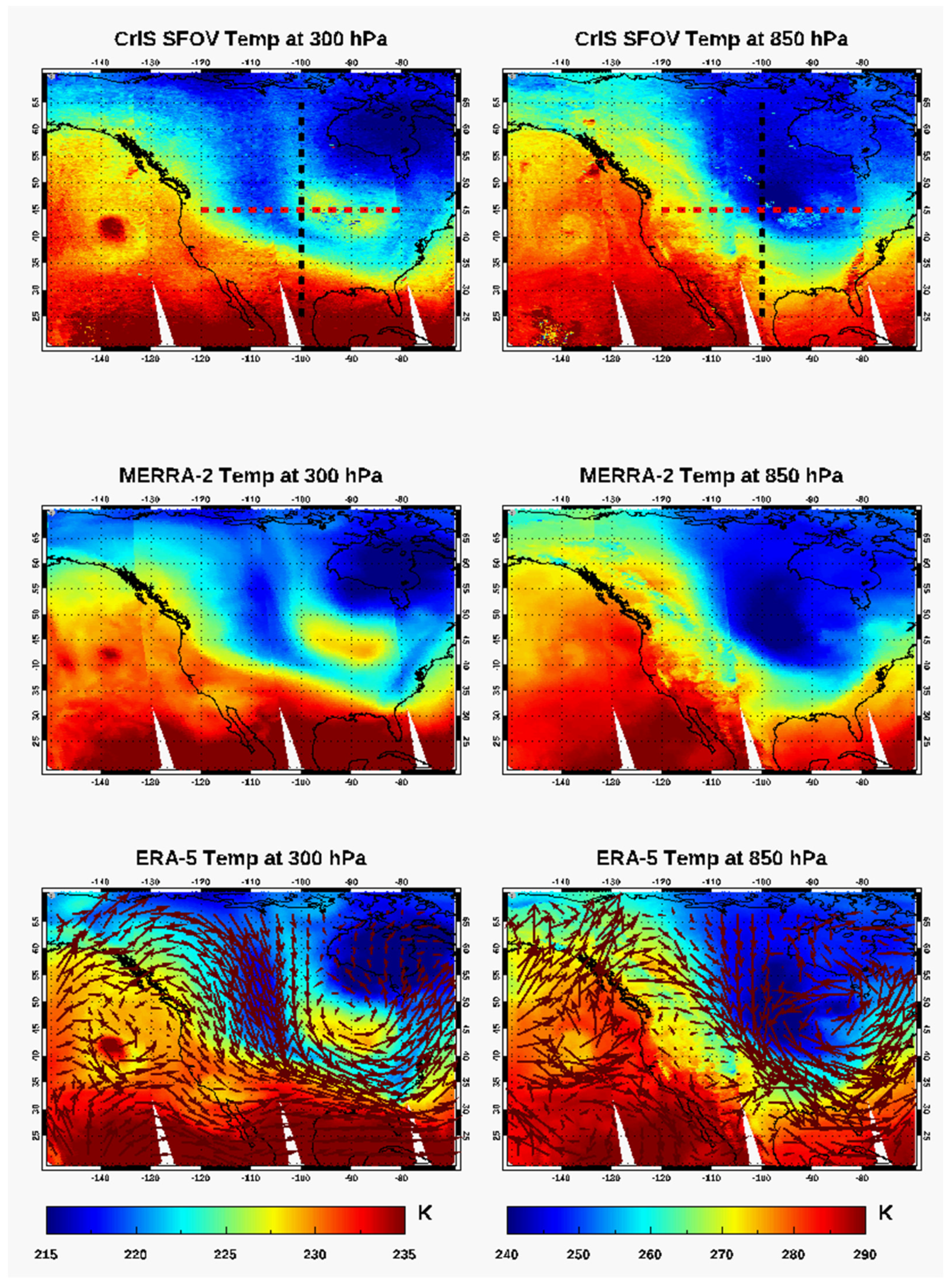
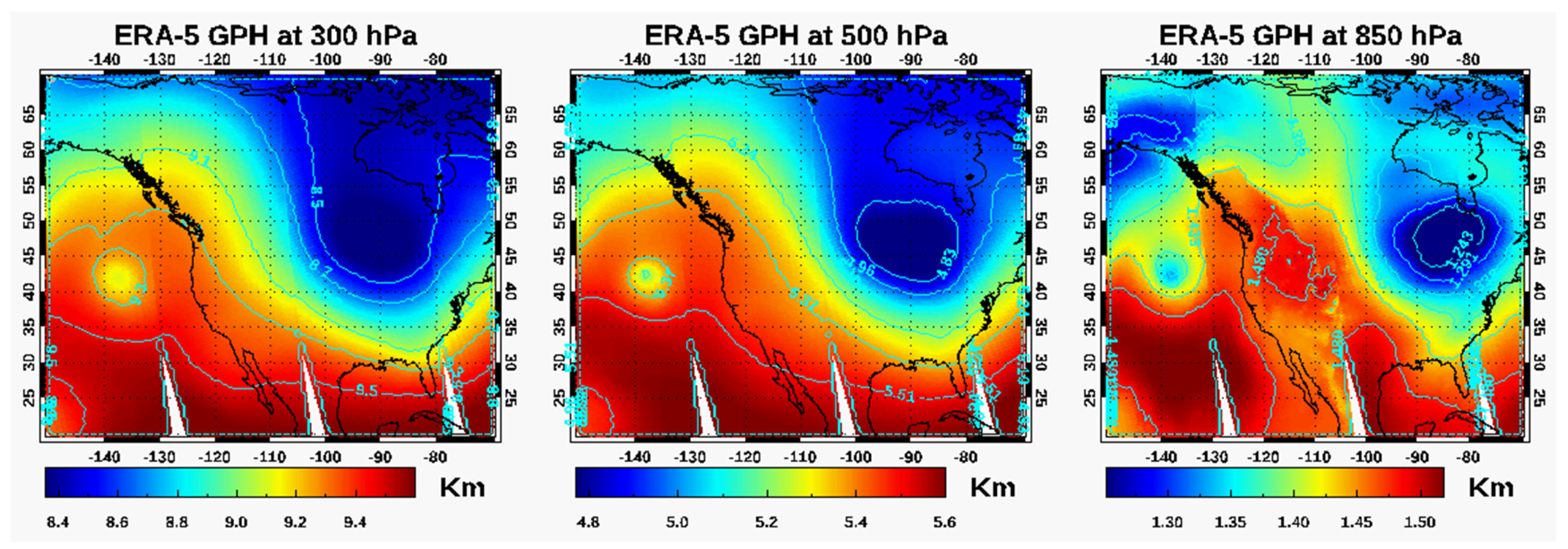
3.1. Distribution of T and GPH at Different Levels and the CAO Transport Path on 29 January 2019

In late January 2019, severe cold waves caused by a weakened jet stream around the Arctic polar vortex hit the Midwestern United States and Eastern Canada, killing at least 22 people. It came after a winter storm brought up to 13 inches (33 cm) of snow in some regions from 27–29 January and brought the coldest temperatures in over 20 years to most locations in the affected region, including some all-time record lows [56]. Using the data from 29 January 2019, Figure 1 shows the distribution of temperature at 300 hPa and 850 hPa impacted by this CAO over North America. Overall, the CrIS SFOV retrieval products and the corresponding ERA-5 and MERRA-2 reanalysis products show very similar patterns to show the cold air blast across a large region in the midwestern United States and Eastern Canada. An interesting feature is that near the region with very cold air temperature at 850 hPa (right panels), a warm area at (100°–80° W, 40°–50° N) is evident at 300 hPa. Some minor differences among them are visible, for example, over the Pacific Ocean off the west coast there is an obvious small warm cyclone center near (142° W, 42° N) at 300 hPa and its size as evident from CrIS is similar to that from ERA-5, but the size from MERRA-2 is much smaller.
From the wind direction in the lower two panels of Figure 1, we can see the southward transport of airmass in the region between 105° W–96° W, which starts to turn counterclockwise between 40° N–50° N. Along this southward transport path (105° W–96° W, 50° N–70° N) the air at 300 hPa is slightly warmer than the air immediately to the east and west and an obvious warm center at 300 hPa forms at (100° W–80° W, 40° N–50° N) with the counterclockwise flow of air (see ERA-5 winds in Figure 1, bottom panel). The location of the 300 hPa warm center is close to the coldest air center at 850 hPa. To better see the distribution of cold airmass in different altitudes, Figure 2 plots the GPH at three levels. It is evident that the location of the coldest air below 850 hPa shifts a little to the east at (98° to 72° W, 40° to 50° N) as compared with the air below 500 hPa. By comparing the GPHs at 300 and 500 hPa (Figure 2), we can also see some slight shift of the cold region (with a low GPH) towards the east between 65–70° N. We also found that the transport path of the dry stratospheric air can be displayed clearly using the CrIS SFOV retrieved RH at 300 hPa, as shown in Figure 3.

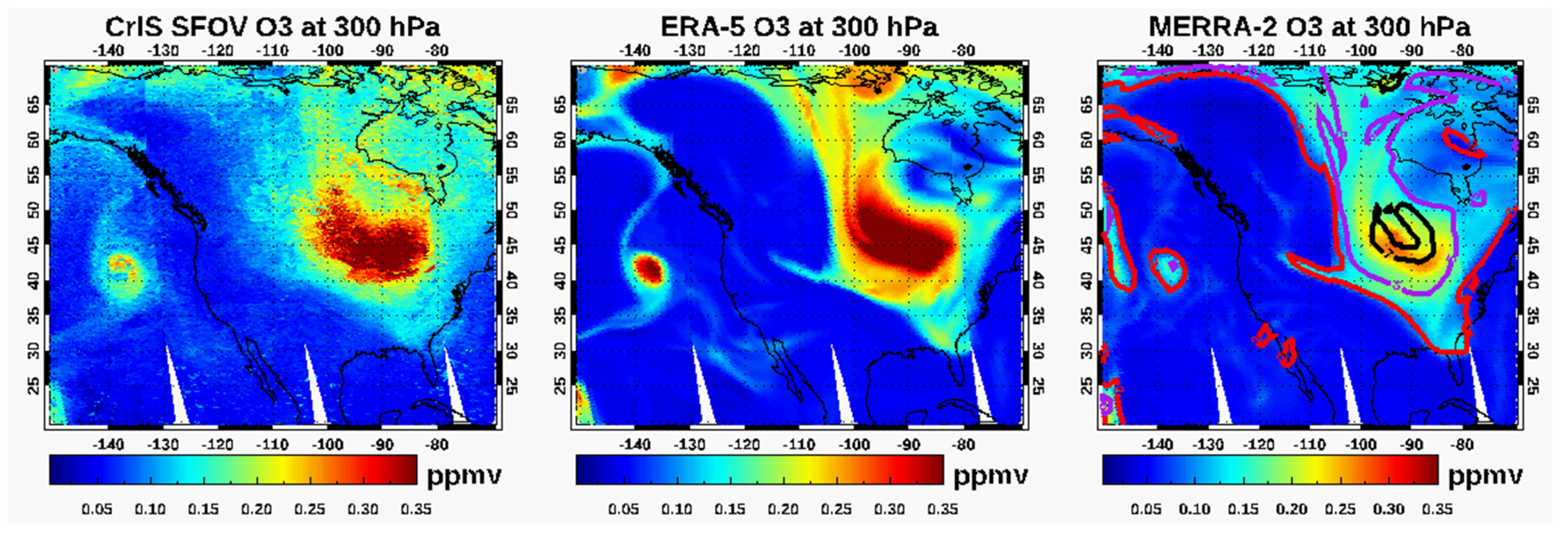
3.2. Enhancement of O3 along the CAO Transport Path and Its Link to Stratospheric Intrusion

As CrIS has a good sensitivity to measure O3 in the UTLS region, O3 at 300 hPa from CrIS can be used to track the stratospheric intrusion to the troposphere [37]. From Figure 4, the enhancement of O3 at 300 hPa is evident along the path of cold air transport and ERA-5 shows more fine features. Plots of the PV contours from MERRA-2 (right panel) further confirm the link of the cold air transport with stratospheric intrusion, as the PV = 2 PVU contour usually marks the boundary of dynamic tropopause, and the contour lines of 5 and 7 PVU indicate that the airmass along the transport path and over the coldest surface center is largely from the stratosphere (Figure 4). The purple PV line has a good match with the transport path mentioned above and within it the O3 concentration is greater than 150 ppbv (parts per billion in volume). The black PV line is near the coldest surface center and the 300 hPa warm center and within it the O3 concentration is greater than 300 ppbv from CrIS SFOV and ERA-5 products.
Enhancement of O3 along the transport of this CAO is also evident from the total column ozone (TCO), as shown in Figure 5. The TCO measured by OMPS shows a similar spatial pattern as those from CrIS SFOV, ERA-5, and MERRA-2 products, however the advantage of the CrIS SFOV O3 product over OMPS is evident by comparing the spatial resolutions in the top two panels of Figure 5. In addition, CrIS provides one night observation that OMPS lacks every day (not shown here). Some quantitatively comparisons of the TCO in the three regions marked in the top right panels as well as the comparison of T and RH will be presented in Section 3.5 and Section 3.6.

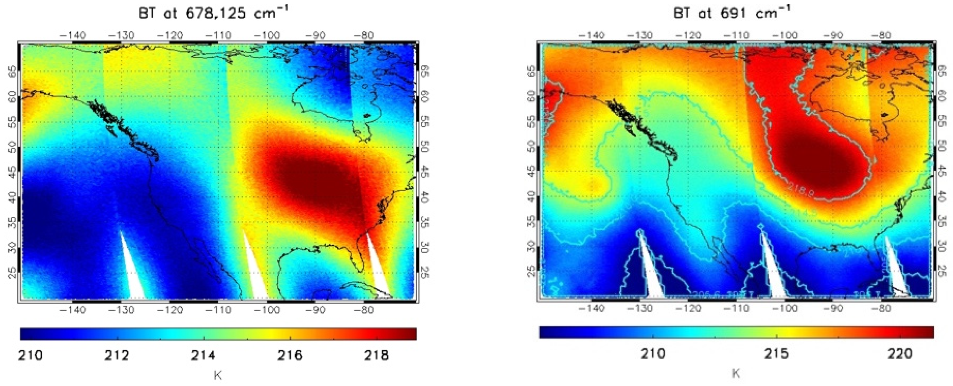
3.3. Upper Warm Center Detected Using CrIS Stratospheric Sounding Channels

Using the Satellite Infrared Spectrometer (SIRS) flown on Nimbus 4, Ghazi [57] first found that the SIRS radiance center at 678 cm−1 is highly correlated with the mean temperature of the stratospheric layer at 100–5 mb (approximately 16–36 km). Following this study by Ghazi [57], Figure 6 plots the brightness temperature (BT) measured by a CrIS stratospheric sounding channel at 678.25 cm−1; obviously the location of the warm center is correlated with the location with the largest enhancement of O3 at 300 hPa and TCO. Such a positive correlation was first found by Ghazi [57]. A similar positive correlation between TCO and polar lower stratospheric temperature resulting from a sudden stratospheric warming (SSW) was also found by Madhu [58], but they observed a negative correlation between O3 concentration and stratospheric temperature in the middle latitude regions. Using another stratospheric sounding channel at 691 cm−1, which measures thermal radiance from a layer lower than 678.25 cm−1, the warming center is still evident, but the location has slightly shifted and some warm air is evident along the transport (middle panel). However, if using the BT at channel 668 cm−1, whose sensitivity is at a higher altitude at 30 hPa and above, the warm center is invisible (not shown), suggesting the warming of the stratosphere only occurs below 30 hPa. Along the transport path (105–96° W, 50–70° N) and over the warm center (100–80° W, 40–50° N), the low RH (<30%) (see Figure 3) is correlated with the contour of BT at 218.9 K. The location of this warm center from the BT at 691 cm−1 is also very close to the warm center of temperature at 300 hPa (bottom left panel of Figure 1). More analysis later in this paper will provide more evidence to demonstrate that the forming of the warming center is caused by the downward transport of the warming airmass in the lower stratosphere. Please note that, in general, it is hard to tell the accurate altitude of this warm center based on the BTs in one or two CrIS sounding channels, and the CrIS SFOV retrieved temperature products should be used instead.

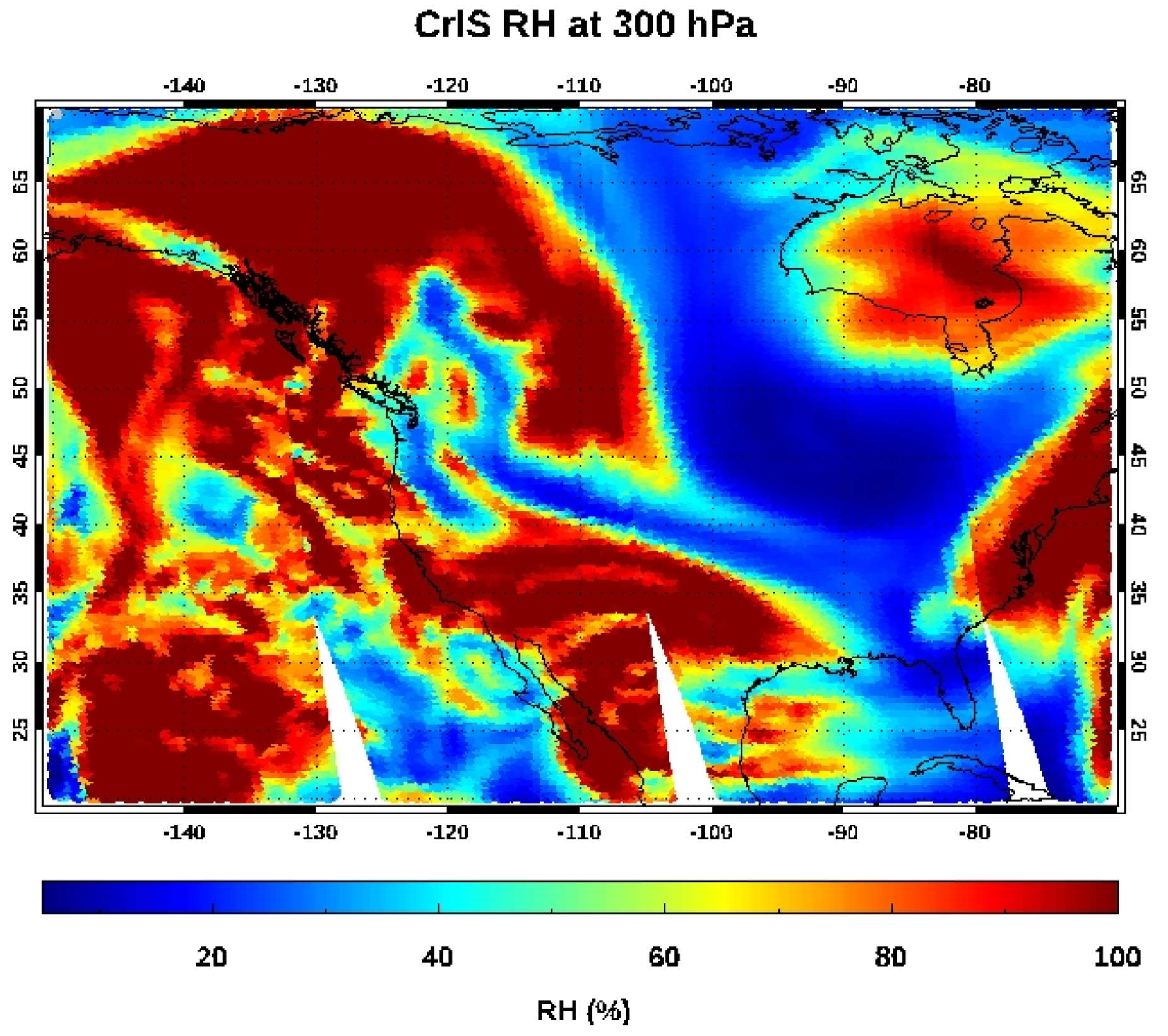
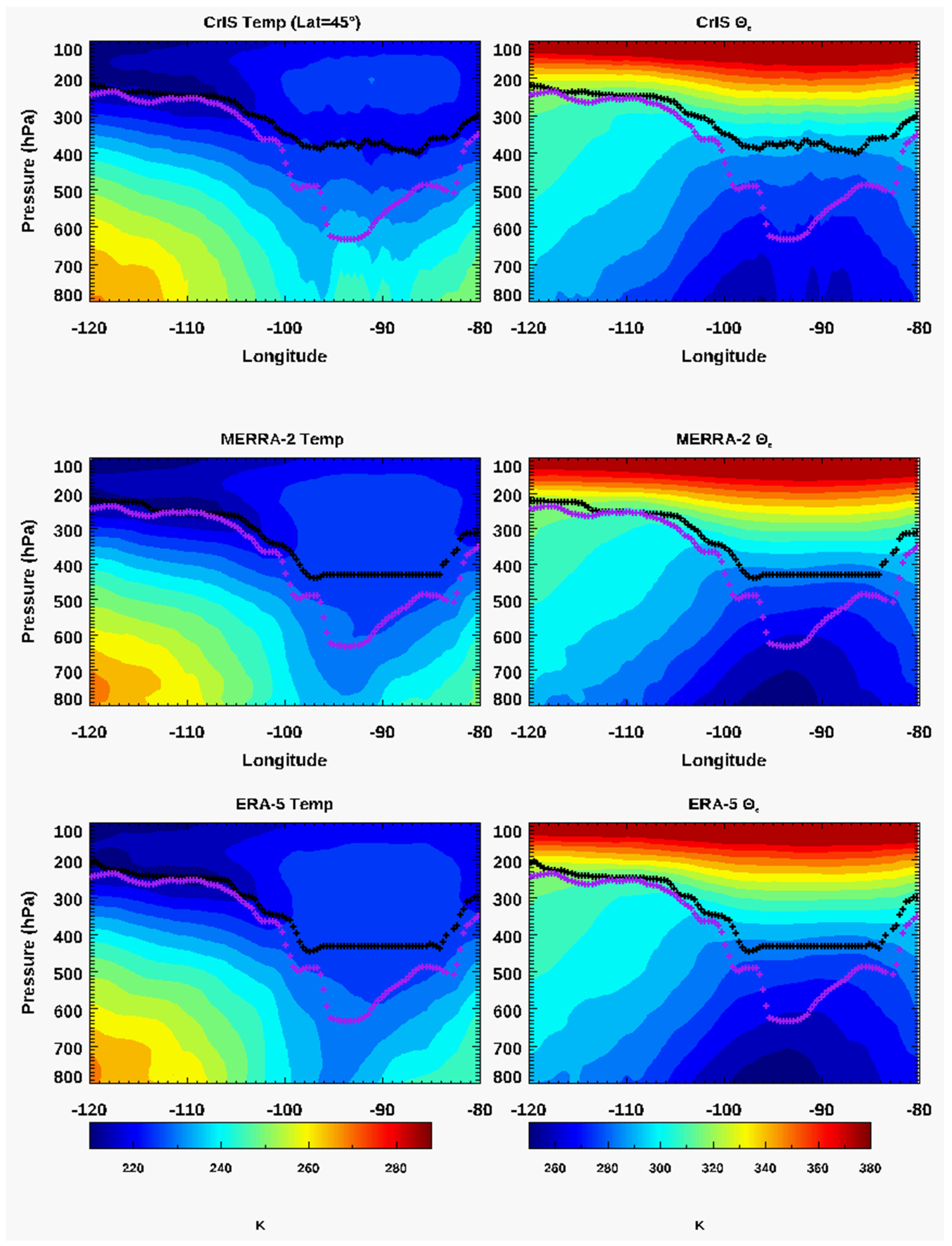
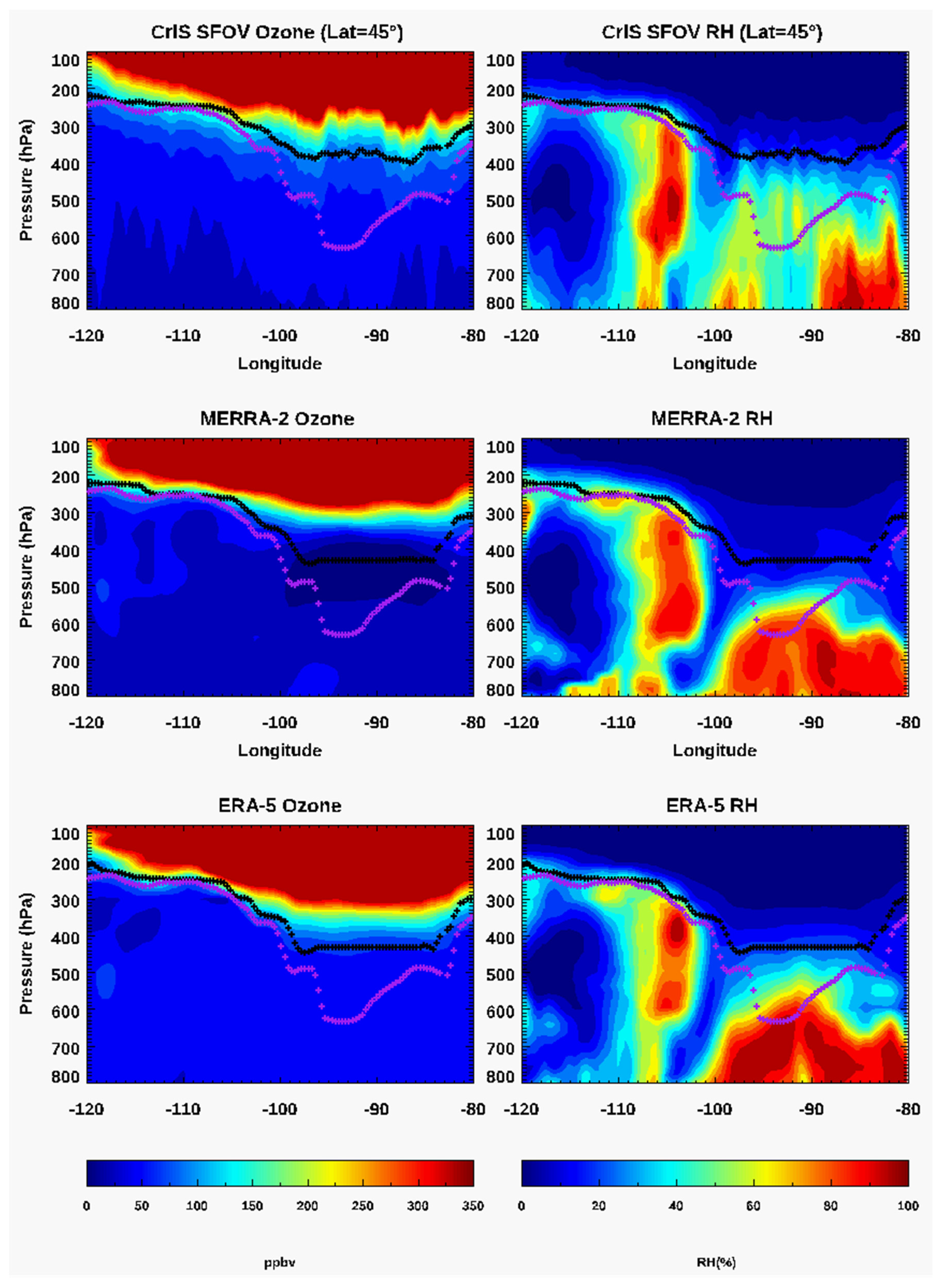
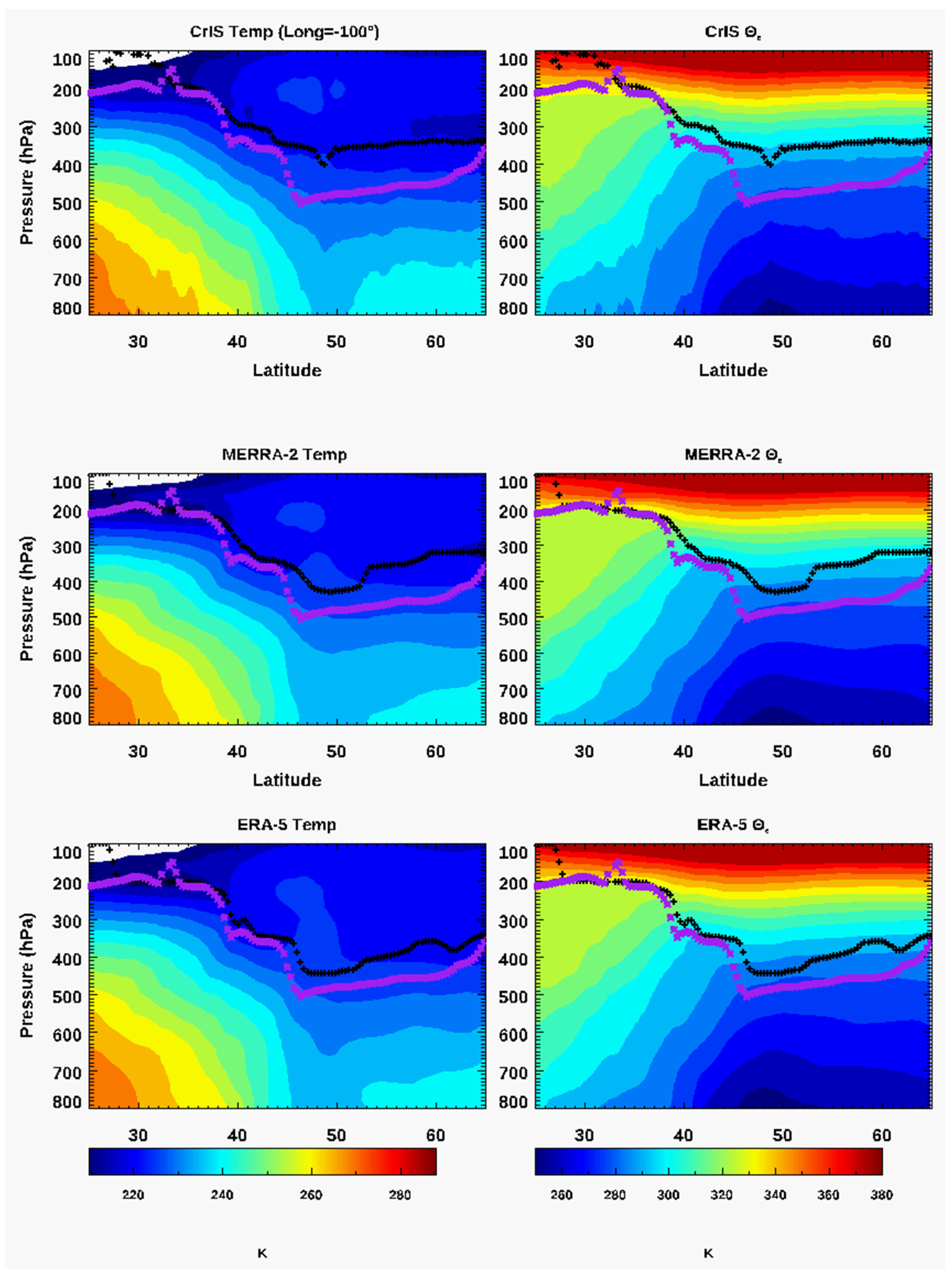
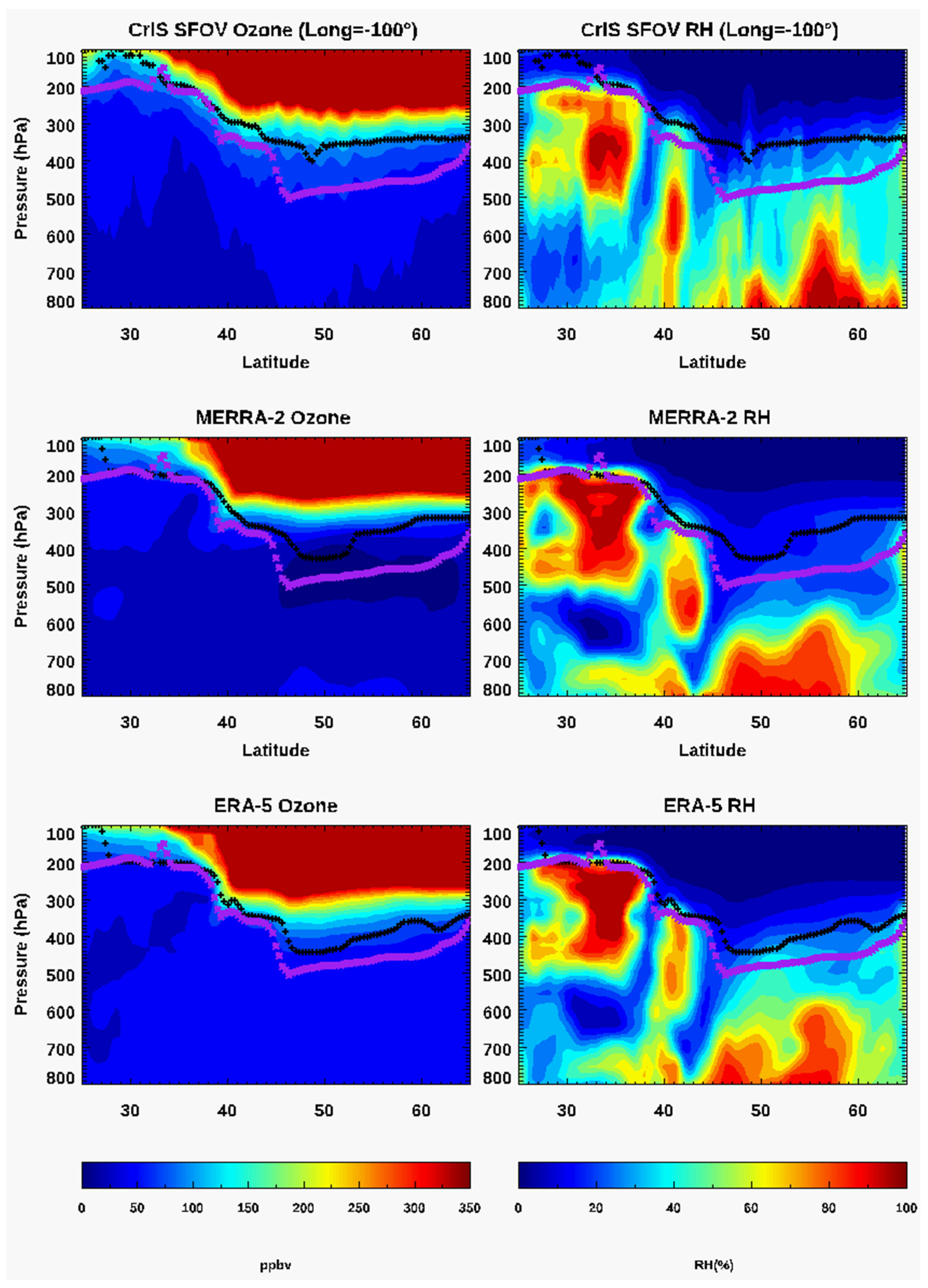
3.4. Analysis of Stratospheric Air Downward Transport Using the Cross-Sections of T, RH, and O3

To better understand the transport in a vertical direction, Figure 7 plots the longitude-pressure cross-section of T and the equivalent potential temperature (Θe) from 120–80° W along 45° N (red dash line in Figure 1). For comparison, both the thermal tropopause (calculated using different T profiles) and the dynamic tropopause (using MERRA-2 data only) are plotted. A large difference in the two tropopause heights is evident between 100–80° W, where the altitude of the dynamic tropopause is much lower than that of the thermal tropopause. Between 90–97° W, the dynamic tropopause is below 550 hPa, indicating that a deep stratospheric intrusion occurred in this area. The pattern of the change of temperature gradient with longitude, overall, follows the pattern of downward intrusion of the dynamic tropopause, with the lowest dynamic tropopause in the coldest region between 100–90° W (at 800 hPa), suggesting the link of stratosphere intrusion with CAO. In the region with low dynamic tropopause (purple crosses) (>500 hPa), a warm air above the thermal tropopause (dark crosses) is evident from the CrIS SFOV product and the two reanalysis products. The pattern of this warm center above the tropopause is similar to that found by Tao et al. [59] using the simulations by the Weather Research and Forecasting (WRF) model, where the upper troposphere–lower stratosphere warm temperature anomaly distribution is resulted from the stratospheric vortex downward intrusion [59].
Some previous studies have used the potential temperature and shown that within the tropopause folding region (tropopause folding refers to a process in which a thin band of stratospheric air intrudes more or less deeply into the troposphere along the strongly titled isentropes associated with an upper tropospheric frontal zone [50]), the transport of stratospheric O3 occurred along the downward sloping isentropes (lines of constant potential temperature) [50,60]. The equivalent potential temperature (Θe), in which both the temperature and the moisture are considered, has also been used in some other studies [61,62], and by using Θe, the drier stratospheric air may be more easy to separate from the moist tropospheric air than using Θ. Hence, in Figure 7 we plotted the equivalent potential temperature longitude-pressure cross-sections along with the cross-sections of temperature. From Figure 7, it is evident that the contours of Θe dip down to the west of 102° W and to the east of 82° W. Such a transport of stratospheric air along the downward sloping isentropes of Θe is also evident from the RH (Figure 8), particularly the downward path with a very low RH from (400 hPa, 100° W) towards (800 hPa, 104° W). As suggested by Xiong et al. [37], RH is better to be used to illustrate the depth of transport than O3 due to the limited sensitivity of CrIS to O3 in the lower atmosphere. From the RH in Figure 8, it is evident that the intrusion depth of stratospheric dry airmass between 95–85° W is at ~430 hPa from CrIS and ERA-5, and ~500 hPa from MERRA-2. The filament of deep dry air transport in the west of 100° W is well captured by CrIS, ERA-5, and MERRA-2. Some thinner downward transport of dry air in the east of 82° W is also evident from CrIS and the two reanalysis products, even though the agreement between them is a little worse. Overall, the cross-section of RH shows a finer structure of the dry air transport from stratosphere to troposphere than what is shown from the O3 cross-sections. Between 98–82° W, the intrusion depth from O3 almost equals that from RH in both CrIS SFOV and ERA-5 products, but MERRA-2 shows a large disparity, with a thin O3 enhancement layer and a thick dry layer.
From the comparison of the patterns shown in Figure 7 and Figure 8, it is evident that the agreement of temperature among CrIS SFOV, ERA-5, and MERRA-2 (Figure 7) is relatively better than the agreement of O3 and RH (Figure 8). From the cross-sections of O3 and RH, the ERA-5 is overall in a better agreement with CrIS SFOV retrievals than MERRA-2. One obvious feature is in the layer below the thermal tropopause and above the dynamic tropopause; MERRA-2 has a thicker dry layer than CrIS and ERA-5. The disparity of RH between these two reanalysis products with the CrIS retrieval products may indicate some disparity between these two assimilation model systems. It should be noted that some difference of their products can be attributed to the observation data assimilated in their systems. For example, radiosondes have been widely used in the data assimilation system. Vaisala RS41 radiosondes have replaced RS92 to become the dominant radiosonde type in the upper air network. In a recent study by Sun et al. [61], they found the standard RS92 may have a dry bias of 3–4% and RS41 may still have a dry bias of 1–1.5% for both daytime and nighttime. Compared with Infrared Atmospheric Sounding Interferometer (IASI) measurements, Sun et al. [63] also pointed out that the simulated radiances using ERA-5 match better than those using radiosondes is perhaps because ECMWF assimilates IASI measurements. These results demonstrate the capability to use the SFOV product to capture the thermodynamic structure impacted by CAO events, which may help us to better understand the dynamic transport and help model evaluation. Further analysis of their difference is important for improving their model for climate analysis and weather forecasting, but this is out of the scope of this paper. In this instance, CrIS SFOV products may be a valuable observational-based dataset for their evaluation.
In order to have a picture of the meridional transport, we also plotted the latitude-pressure cross-sections of T, Θe, O3, and RH along 100° W (along the black dash line in Figure 1) in Figure 9. The largest gradient of tropopause change occurred at (35–46° N). At ~46° N the dynamic tropopause reached its lowest height of 500 hPa, where a significant decrease of temperature in the layers under the tropopause until the lower troposphere is evident. This pattern is due to the transport of cold air from the north, blocked by the warm air from the south to form a shear near 40° N (see the wind fields at the bottom panels of Figure 1). The largest gradient of Θe also suggests the transport of stratospheric air along the downward-sloping isentropes of Θe between 35–42° N, where we can also see the formation of warm air between 40°–57° N above the thermal tropopause. At 800 hPa, the location of the coldest area is between 46°–53° N. From the RH in Figure 10, the path of the downward transport of the dry stratospheric air from (400 hPa, 46° N) down to (800 hPa, 42° N) is evident. Another filament of the downward transport path from (250 hPa, 39° N) down to (700 hPa, 36° N) is also evident from the cross-section of RH, which is associated with a dip of the dynamic tropopause to ~300–350 hPa ner ~38° N. Similar to that shown in Figure 8, it is evident from Figure 10 that MERRA-2 has a thicker dry layer (i.e., a low RH) below the thermal tropopause than CrIS and ERA-5 data in the region between 45–60° N, and the stratospheric intrusion depth shown from O3 disagrees with that shown from RH.

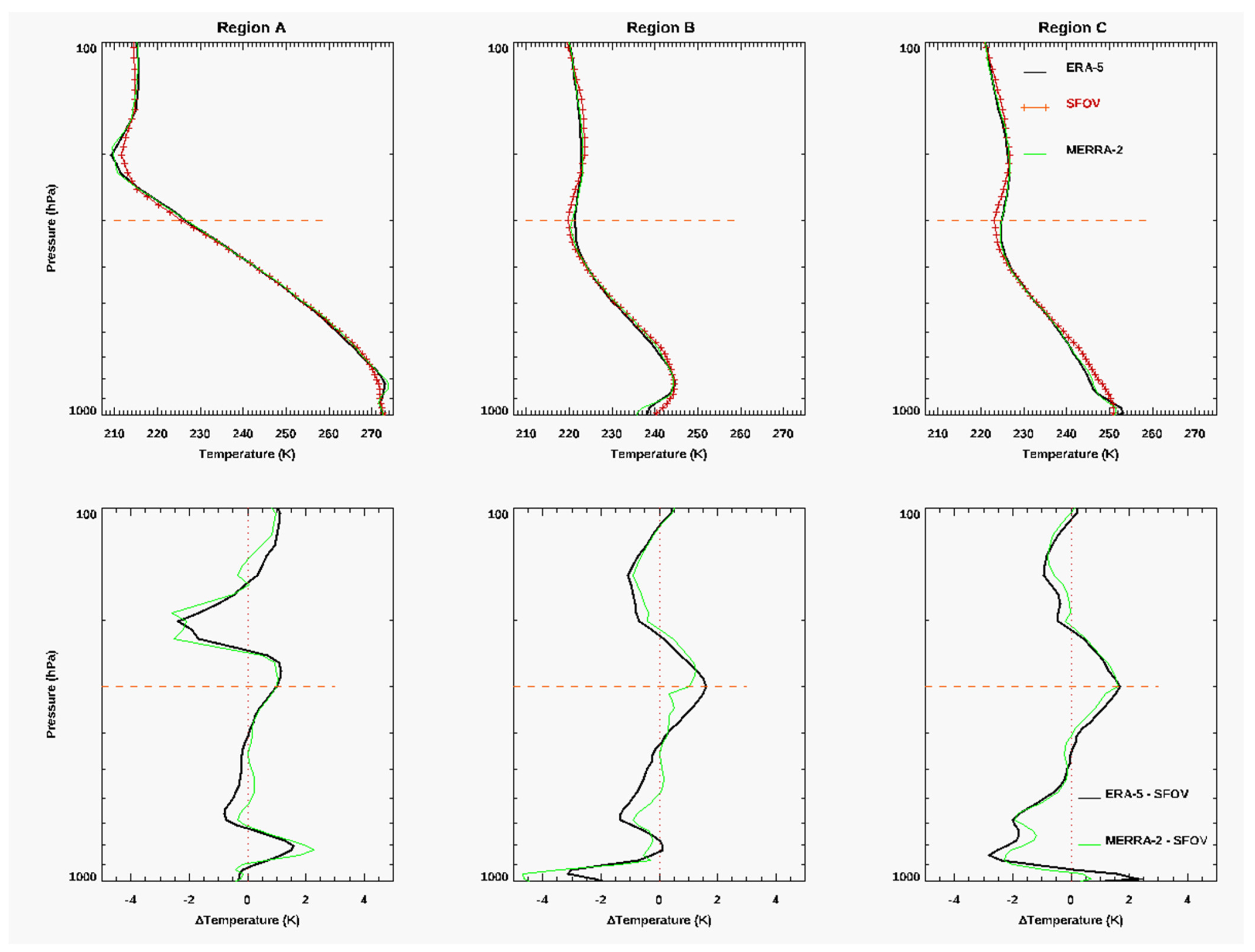
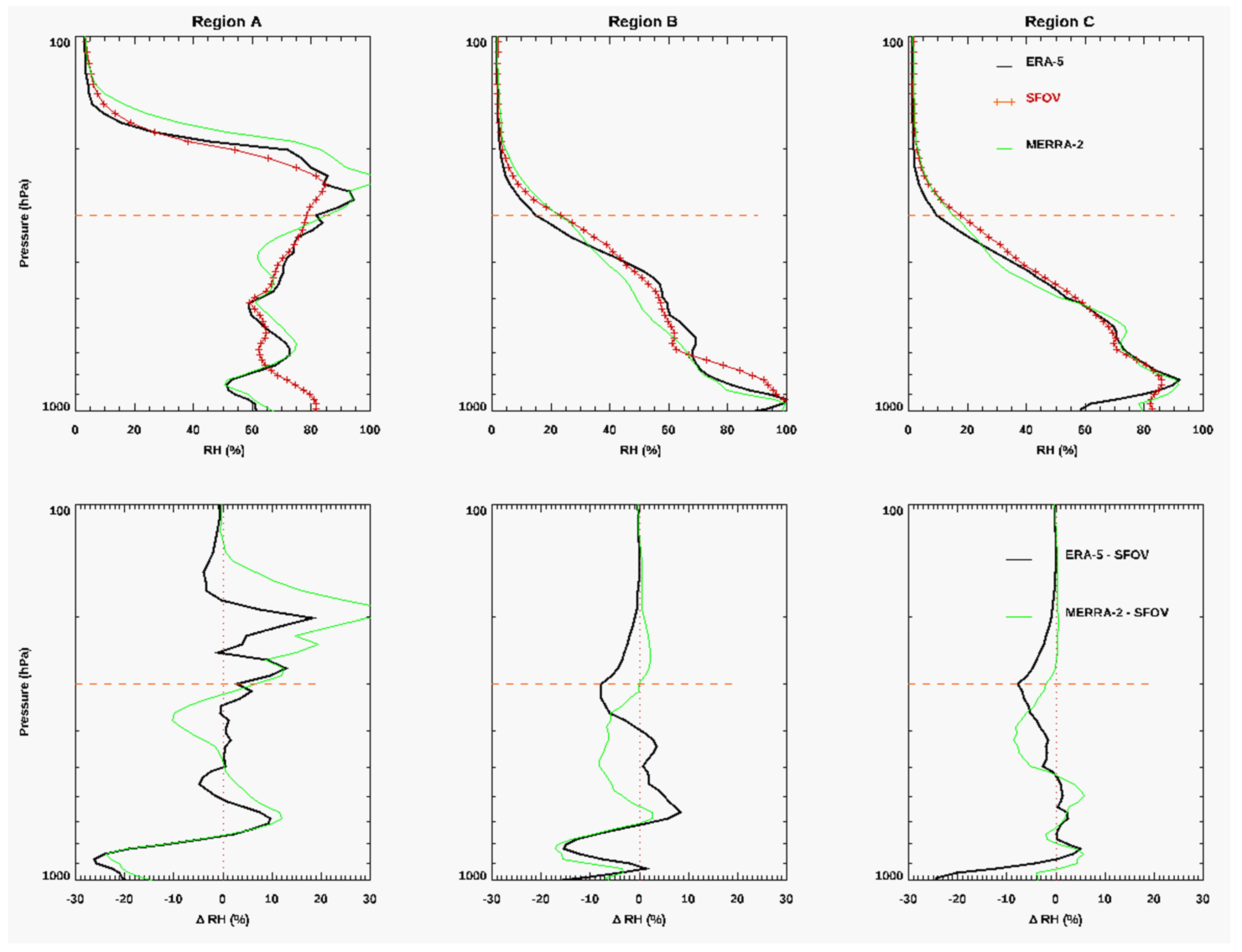
3.5. Comparison of T and RH Profiles from CrIS SFOV with ERA-5 and MERRA-2

To further analyze the impact of CAO on the change of T and RH profiles along the transport pathways and to quantify the performance of CrIS SFOV retrievals and the ERA-5 and MERRA-2 reanalysis products in this extreme weather condition, we selected three regions, as shown in Figure 5, and compared the mean T and RH profiles. As shown in Figure 11, in region A, which is outside the CAO impacted region, the mean temperature decreases with altitude and reaches the minimum at ~200 hPa. Under the impact of CAO, the level with the minimum of temperature moves down to ~300 hPa in region B and moves to an even lower altitude in region C. In the CAO impacted regions B and C, a large increase of temperature in the order of 10 K is evident in the layer between 100–200 hPa as compared with region A, showing the warming in the lower stratosphere. Based on the CrIS SFOV retrievals, at 200 hPa the mean temperatures increase from 211.6 K (in region A) to 223.7 K (in region B) and 226.3 K (in region C). The location with the lowest temperature around 300 hPa is roughly the location of thermal tropopause, and it is evident that the tropopause in region C is slightly lower than in region B from the top right two panels of Figure 11. Near the surface, the temperature at 950 hPa is 272.4 K (in region A) and it decreases to 241.8 K (in region B). In region B, an inversion layer below 850 hPa from CrIS SFOV, ERA-5, and MERRA-2 suggests that the advection of polar cold air plays an important role in impacting the surface temperature along the transport path of cold air.
Figure 11 shows the mean difference of the matchup temperature profiles from ERA-5 and MERRA-2 minus the CrIS SFOV retrieval profiles (bottom panels). It is evident that in the CAO-impacted regions B and C, the temperature at 300 hPa from ERA-5 and MERRA-2 is warmer than the CrIS SFOV product by 1.0 K to 1.5 K, while the difference between ERA-5 and MERRA-2 is much smaller. As expected, the difference of the surface temperature from the CrIS SFOV retrieval with both reanalysis data is a little larger than in the upper troposphere layers and this uncertainty is partially associated with the uncertainty in the retrieval of surface emissivity. This difference is similar to one previous validation to AIRS and/or NUCAPS products [38], suggesting the quality of the CrIS SFOV temperature product in this extreme CAO conditions is reasonably good as compared with MERRA-2 and ERA-5 reanalysis products. However, the relatively larger difference at the tropopause needs more investigation.
From the vertical profile of RH in Figure 12, it is evident that the mean RH in region A is >70–80% in the layer above 300–200 hPa, indicating it is the tropospheric air at ~200 hPa. Due to the descending of stratospheric dry air (RH < 30%), in regions B and C the air at 300 hPa is clearly from the stratosphere as the SFOV RH and MERRA-2 RH is about 28 and 20%, respectively, and the ERA-5 RH is even 5–6% less. The transport of stratospheric air is extending to 350–400 hPa (RH < 30%). From the RH differences, it is evident that the disparity of RH between ERA-5 and MERRA-2 can be as large as 10%, showing the agreement of the RH product from the two reanalysis data is not as good as their temperature products. The difference of CrIS SFOV RH with ERA-5 and MERRA-2 is within the range of 10–20% in the CAO-impacted regions (B and C), which is comparable with previous validation of AIRS and/or NUCAPS products [38]. In the CAO-impacted regions B and C, the RH from MERRA-2 is less than CrIS SFOV and ERA-5 by 5–10% layer between 400–550 hPa, which is consistent with the previous finding of a thick dry layer under the tropopause (see Figure 8 and Figure 10). A relatively larger disparity of T and RH in region A can be partially attributed to the use of data along the coast, where the retrieval uncertainty is usually relatively larger.

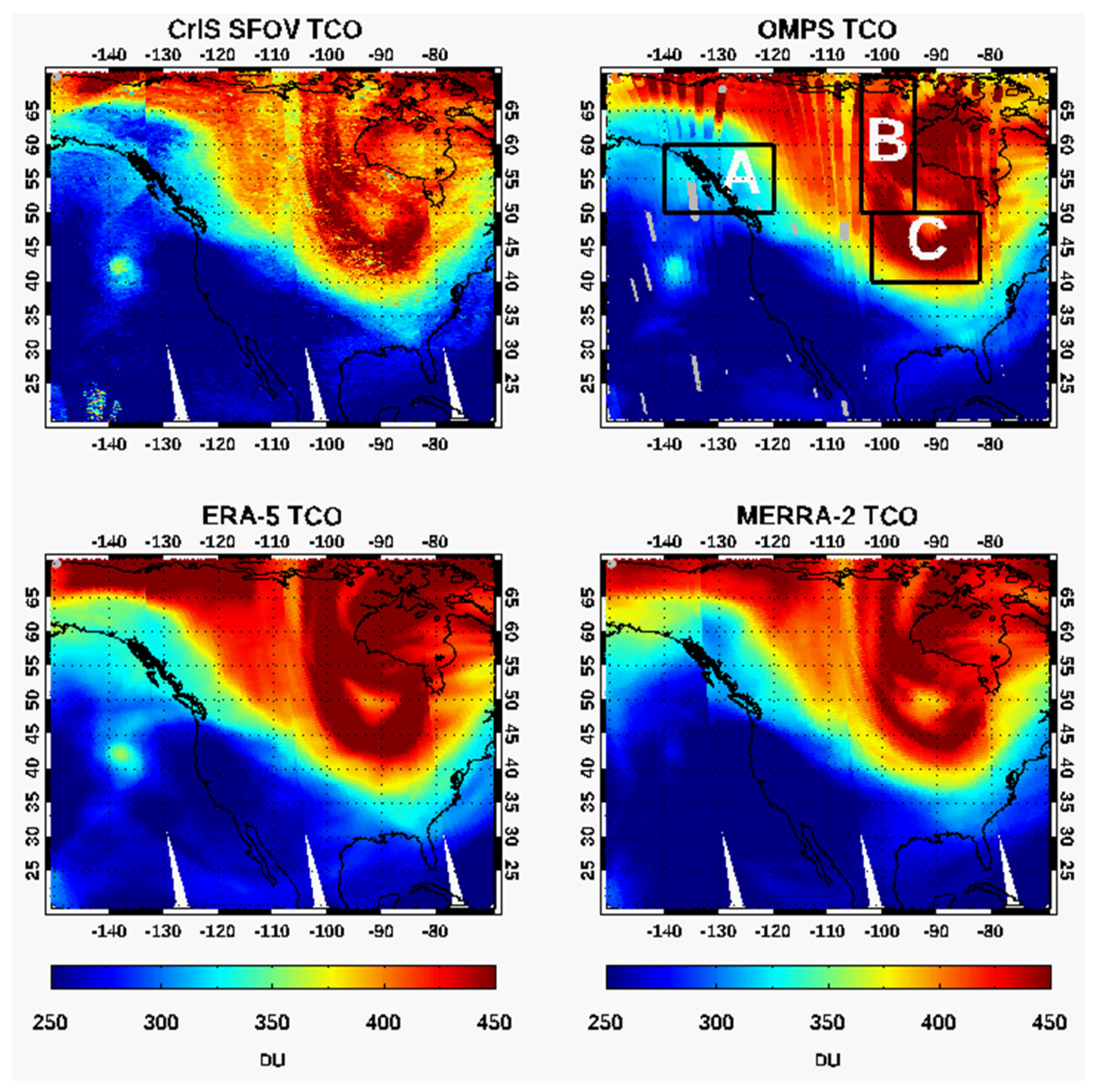
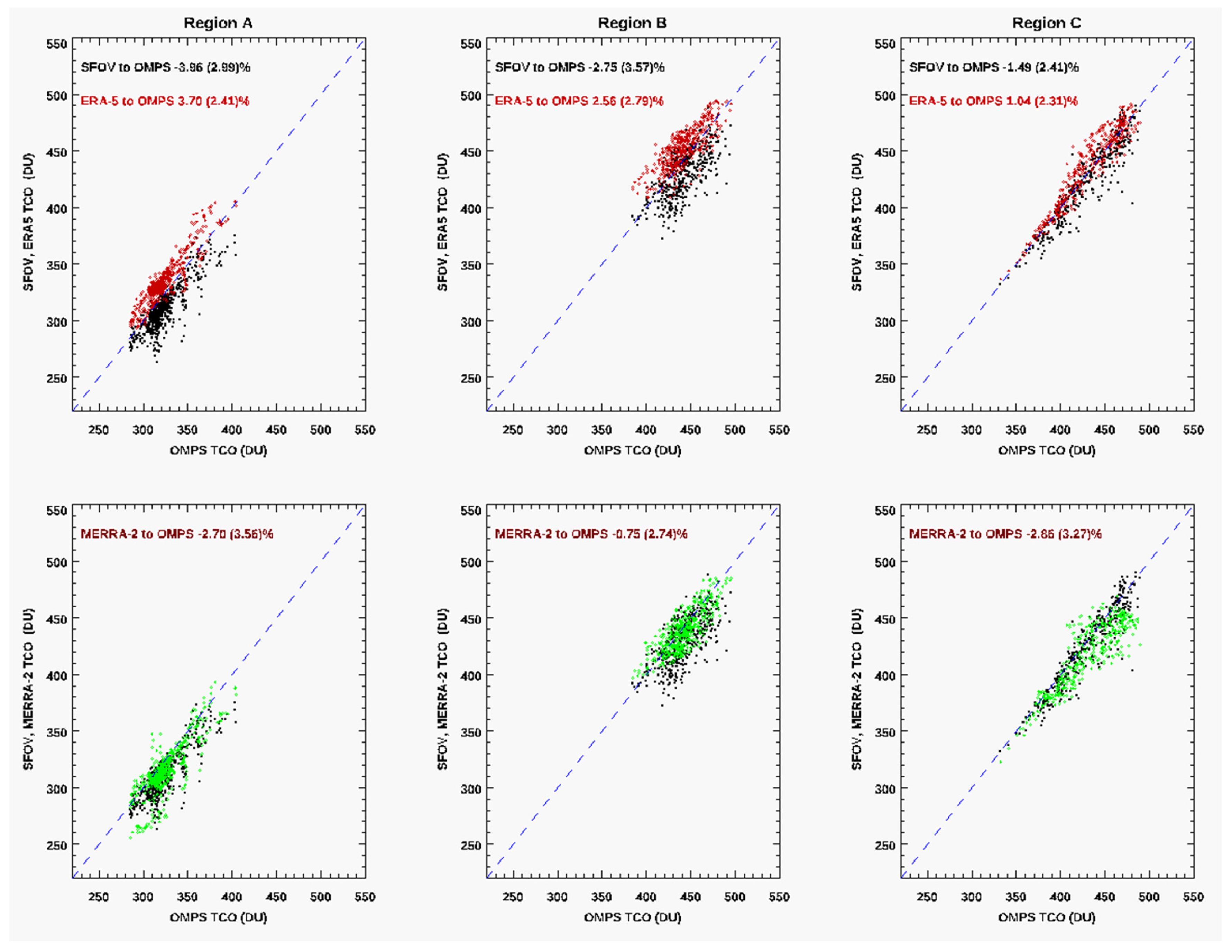
3.6. Comparison of TCO from ERA-5, MERRA-2, CrIS SFOV with OMPS

The TCO from OMPS on S-NPP is used as a standard to compare against the TCO from CrIS SFOV, MERRA-2, and ERA-5 reanalysis data in the same three regions as before. As shown in Figure 13, overall across these three regions the SFOV TCO has a better agreement with MERRA-2 than with ERA-5, and the ERA-5 TCO is biased high compared with OMPS, while SFOV and MERRA-2 are biased low. In the CAO-impacted region C, the errors of CrIS FOV, MERRA-2, and ERA-5 TCO relative to OMPS TCO are −1.29 ± 2.32%, −2.79 ± 3.12%, and 1.06 ± 2.32%. By using all the co-located data in the whole image shown in Figure 4, the errors of CrIS FOV, MERRA-2, and ERA-5TCO relative to OMPS TCO are −2.5 ± 3.2%, −1.0 ± 3.8%, and 2.8 ± 2.8%, respectively. This estimated error of MERRA-2 is consistent with the study of Wargan et al. [64] that compared MERRA-2 total ozone with TOMS data (1980–1993) and found their difference is less than 2% in bias and less than 6% in standard deviation. The finding of a positive bias of ERA-5 TCO, as compared with OMPS and MERRA-2, is consistent with the finding by Xiong et al. [37].

4. Summary and Conclusions

An extreme CAO event that occurred during 28–31 January 2019 was examined with a focus to understand the impact of the stratosphere to the surface cold air transport. In this study, the distributions of T, RH, and O3 on 29 January 2019, as well as their cross-sections, were analyzed using the CrIS SFOV retrieval products, a new product from NASA Langley Research Center. For comparison, the corresponding ERA-5 and MERRA-2 reanalysis products were used in the same way. Data of wind, PV, and GPH from ERA-5 and MERRA-2 were used to characterize the dynamic transport of this CAO event. Served as a simple cross-validation to the performance of SFOV retrievals and reanalysis products under this extreme weather condition, some comparison of the SFOV retrieved T and RH profiles with ERA-5 and MERRA-2 products, as well as their TCO with OMPS data, were also made.
It is found that the path of the cold air transport on 29 January 2019 across the US Midwest can be well captured from the wind fields, GPH at 300 and 850 hPa, the map of O3 and RH at 300 hPa, and the map of TCO. Along this cold air transport path, particularly over the coldest center, the source of air at 300 hPa is largely from the stratosphere as the modeled PV is larger than 5 PVU and the O3 concentration is much larger than 150 ppbv, a value used in the chemical tropopause [65]. The downward transport of stratospheric air has been illustrated explicitly from the cross-sections of T, RH, and O3. More fine features of the transport path and the transport depth can be captured using RH, even though the agreement of RH in different models is not so well as their temperature products. In consistent with the observation by Ghazi [57] and the model simulations by Tao et al. [59], a warm center above the tropopause was directly observed using the CrIS stratospheric sounding channels. This warm center is associated with stratosphere warming [57,58] as well as the downward stratospheric transport. While several possible dynamical mechanisms for the downward stratospheric influence on CAO have been proposed from previous studies that were mostly based on model data, such as the link of the large-scale PV anomalies in the lower stratosphere with zonally symmetric zonal wind perturbations extending downward to the earth’s surface, wave propagation, or stratosphere vortex downward intrusion [59], this study provided direct evidence from satellite observations to confirm the impact of the stratosphere to the CAO process through the downward transport.
Overall, CrIS SFOV products and the two reanalysis products perform well to capture the large-scale patterns of T, RH, and O3 associated with this CAO and characterize the tropopause descending and downward isentropic stratosphere-to-troposphere transport. However, compared with the good agreement in T, the disparity of RH can be up to 10% between the two reanalysis products, and it is noteworthy that in the CAO-impacted regions MERRA-2 shows a thicker dry layer below the tropopause than that from the ERA-5 and CrIS SFOV products. Moreover, comparison of TCO with measurement by OMPS show that the ERA-5 TCO has a positive bias of 2.8 ± 2.8%, while CrIS and MERRA-2 TCO have a negative bias of −2.5 ± 3.2% and −1.0 ± 3.8%, respectively. Please note that these differences are only based on one CAO case and should not be overexplained. More validation to CrIS SFOV products using more in situ observations for more cases is ongoing.
This study provides evidence that CrIS observations can be used to identify stratosphere–troposphere coupling and the impact of the stratosphere on synoptic systems, confirming the impact of the stratosphere on CAO through downward transport. It also demonstrated the potential value of CrIS SFOV products, with a high spatial resolution of about 14 km, for observing the thermodynamic state of extreme weather systems like CAO as well as the value for model evaluation. As a new product that will soon become publicly available, the fine-scale three-dimensional variation of T, RH, and O3 as captured from this SFOV products could benefit for future CAO dynamic transport study and likely the assimilation of these SFOV products in the model could help to improve the simulation and forecast of CAO events.

Author Contributions

X.X., X.L., K.E.K. and F.Y. conceived of the presented ideas; the CrIS Single FOV algorithm used in this study was designed and implemented by X.L. and W.W.; X.X. and W.W. were responsible for data collection and processing; X.X., X.L., W.W. and K.E.K. carried out data analysis and interpreted the results; X.X., K.E.K. and X.L. wrote the manuscript with discussion and editing inputs from W.W. and D.K.Z.; Q.Y. is responsible for the update of PCRTM. All authors have read and agreed to the published version of the manuscript.

Funding

This research was funded by the NASA 2017 Research Opportunities in Space and Earth Sciences (ROSES) solicitation NNH17ZDA001N-TASNPP; The Science of Terra, Aqua, and Suomi NPP, and the NASA 2020 ROSES solicitation NNH20ZDA001N; NASA Suomi National Polar-orbiting Partnership (NPP) and the Joint Polar Satellite System (JPSS) Satellites Standard Products for Earth System Data Records.

Institutional Review Board Statement

Not applicable.

Informed Consent Statement

Not applicable.

Data Availability Statement

Data used in this investigation are available at NASA LaRC upon request; SNPP CrIS and ATMS L1B data, AIRS, OMPS L2, and MERRA-2 data were downloaded from NASA DISC: (https://disc.gsfc.nasa.gov/datasets, accessed on 10 January 2021); ERA-5 data were downloaded from ECMWF (https://cds.climate.copernicus.eu/cdsapp#!/dataset/reanalysis-era5-pressure-levels?tab=form, accessed on 10 January 2021).

Acknowledgments

This research was partially supported by the NASA NAST-I program, and the authors wish to acknowledge J. A. Kaye of the NASA Science Mission Directorate for his continued enabling support. Resources supporting this work were provided by the NASA High-End Computing (HEC) Program through the NASA Advanced Supercomputing (NAS) Division at NASA Ames Research Center. K. E. Knowland acknowledges support by the NASA Modeling, Analysis and Prediction (MAP) Program (Project manager David Considine). We would like to thank the four anonymous reviewers for their beneficial comments and suggestions.

Conflicts of Interest

The authors declare that there are no known competing financial interest or personal relationship that could have appeared to influence this paper.

Abbreviations

The following abbreviations are used in this manuscript:
AIRSAtmospheric Infrared Sounder
AMSUAdvanced Microwave Sounding Unit
CAOCold Air Outbreak
CLIMCAPSCommunity Long-term Infrared Microwave Coupled Product System
CrISCross-track Infrared Sounder
DISORTDiscrete Ordinate Radiative Transfer
ECMWFEuropean Centre for Medium-Range Weather Forecasts
ERA-5Fifth generation of ECMWF atmospheric reanalyses of the global climate
FORField of Regard
FOVField of View
GPHgeopotential height
GES DISCGoddard Earth Sciences Data and Information Services Center
IASIInfrared Atmospheric Sounding Interferometer
JPSSJoint Polar Satellite System
MERRA-2The Modern-Era Retrospective Analysis for Research and Applications, Version 2
NAST-INational Aircraft Sounding Testbed-Interferometer
NCARNational Center for Atmospheric Research
NCEPNational Center for Environmental Prediction
NUCAPSNOAA Unique Combined Atmospheric Processing System
NOAANational Oceanic and Atmospheric Administration
NASANational Aeronautics and Space Administration
OMPSOzone Mapping and Profiler Suite
PCPrincipal Components
PCRTMPrincipal Component based Radiative Transfer model
PVPotential vorticity
RHRelative humidity
SIRSSatellite Infrared Spectrometer
SFOVSingle Field of View
SIPSScience Investigator-led Processing System
SNPPSuomi National Polar-orbiting Partnership
UTLSUpper Troposphere and Lower Stratosphere
WMOWorld Meteorological Organization
WRFWeather Research and Forecasting model

References

  1. Walsh, J.E.; Phillips, A.S.; Portis, D.H.; Chapman, W.L. Extreme cold air outbreaks in the United States and Europe, 1948–1999. J. Clim. 2001, 14, 2642–2658. [Google Scholar] [CrossRef]
  2. Cellitti, M.P.; Walsh, J.E.; Rauber, R.M.; Portis, D.H. Extreme cold air outbreaks over the U.S., the polar vortex, and the large-scale circulation. J. Geophys. Res. Atmos. 2006, 111, D02114. [Google Scholar] [CrossRef]
  3. Smith, E.T.; Sheridan, S.C. The characteristics of extreme cold events and cold air outbreaks in the eastern United States. Int. J. Climatol. 2018, 38, e807–e820. [Google Scholar] [CrossRef]
  4. Vavrus, S.; Walsh, J.E.; Chapman, W.L.; Portis, D. The behavior of extreme cold air outbreaks under greenhouse warming. Int. J. Climatol. 2006, 26, 1133–1147. [Google Scholar] [CrossRef]
  5. Intergovernmental Panel on Climate Change (IPCC). Climate Change 2007: The Physical Science Basis. Contribution of Working Group I to the Fourth Assessment Report of the Intergovernmental Panel on Climate Change; Solomon, S., Qin, D., Manning, M., Chen, Z., Marquis, M., Averyt, K.B., Tignor, M., Miller, H.L., Eds.; Cambridge University Press: New York, NY, USA, 2007. [Google Scholar]
  6. Portis, D.H.; Cellitti, M.P.; Chapman, W.L.; Walsh, J.E. Low-frequency variability and evolution of North American cold air outbreaks. Mon. Weather Rev. 2006, 134, 579–597. [Google Scholar] [CrossRef]
  7. Uppala, S.M.; Kållberg, P.W.; Simmons, A.J.; Andrae, U.; Da Costa Bechtold, V.; Fiorino, M.; Gibson, J.K.; Haseler, J.; Hernandez, A.; Kelly, G.A.; et al. The ERA-40 Re-analysis. Q. J. R. Meteorol. Soc. 2005, 131, 2961–3012. [Google Scholar] [CrossRef]
  8. Wheeler, D.D.; Harvey, V.L.; Atkinson, D.E.; Collins, R.L.; Mills, M.J. A climatology of cold air outbreaks over North America: WACCM and ERA-40 comparison and analysis. J. Geophys. Res. Atmos. 2011, 116, D12107. [Google Scholar] [CrossRef]
  9. Kalnay, E.; Kanamitsu, M.; Kistler, R.; Collins, W.; Deaven, D.; Gandin, L.; Iredell, M.; Saha, S.; White, G.; Woollen, J.; et al. The NCEP/NCAR 40-year reanalysis project. Bull. Am. Meteorol. Soc. 1996, 77, 437–471. [Google Scholar] [CrossRef] [Green Version]
  10. Hans, H.; Bill, B.; Paul, B.; Shoji, H.; András, H.; Joaquín, M.S.; Julien, N.; Carole, P.; Raluca, R.; Dinand, S.; et al. The ERA5 Global Reanalysis. Q. J. R. Meteorol. Soc. 2020, 146, 1999–2049. [Google Scholar] [CrossRef]
  11. Smith, E.T.; Sheridan, S.C. Where do cold air outbreaks occur, and how have they changed over time? Geophys. Res. Lett. 2020, 47, e2020GL086983. [Google Scholar] [CrossRef]
  12. Hartley, D.E.; Villarin, J.T.; Black, R.X.; Davis, C.A. A new perspective on the dynamical link between the stratosphere and troposphere. Nature 1998, 391, 471–474. [Google Scholar] [CrossRef]
  13. Kidston, J.; Scaife, A.A.; Hardiman, S.C.; Mitchell, D.; Butchart, N.; Baldwin, M.P.; Gray, L. Stratospheric influence on tropospheric jet streams, storm tracks and surface weather. Nat. Geosci. 2015, 8, 433–440. [Google Scholar] [CrossRef]
  14. Kretschmer, M.; Cohen, J.; Matthias, V.; Runge, J.; Coumou, D. The different stratospheric influence on cold-extremes in Eurasia and North America. NPJ Clim. Atmos. Sci. 2018, 1, 44. [Google Scholar] [CrossRef] [Green Version]
  15. Kretschmer, M.; Coumou, D.; Agel, L.; Barlow, M.; Tziperman, E.; Cohen, J. More-persistent weak stratospheric polar vortex states linked to cold extremes. Bull. Am. Meteorol. Soc. 2018, 99, 49–60. [Google Scholar] [CrossRef]
  16. Thompson, D.W.J.; Baldwin, M.P.; Wallace, J.M. Stratospheric connection to Northern Hemisphere wintertime weather: Implications for prediction. J. Clim. 2002, 15, 1421–1428. [Google Scholar] [CrossRef]
  17. Tanaka, H.L.; Milkovich, M.L. A heat budget analysis of the polar troposphere in and around Alaska during the abnormal winter of 1988/1989. Mon. Weather Rev. 1990, 118, 1628–1639. [Google Scholar] [CrossRef] [Green Version]
  18. Curry, J. The contribution of radiative cooling to the formation of cold-core anticyclones. J. Atmos. Sci. 1987, 44, 2575–2592. [Google Scholar] [CrossRef] [Green Version]
  19. Tan, Y.C.; Curry, J.A. A diagnostic study of the evolution of an intense North American anticyclone during winter 1989. Mon. Weather Rev. 1993, 121, 961–975. [Google Scholar] [CrossRef] [Green Version]
  20. Colucci, S.J.; Baumhefner, D.P.; Konrad, C.E., II. Numerical prediction of a cold-air outbreak: A case study with ensemble forecasts. Mon. Weather Rev. 1999, 127, 1538–1550. [Google Scholar] [CrossRef]
  21. Thompson, D.W.J.; Wallace, J.M. Regional climate impacts of the Northern Hemisphere annular mode. Science 2001, 293, 85–89. [Google Scholar] [CrossRef] [Green Version]
  22. Rogers, J.C.; Rohli, R.V. Florida citrus freezes and polar anticyclones in the Great Plains. J. Clim. 1991, 4, 1103–1113. [Google Scholar] [CrossRef]
  23. Scaife, A.A.; Knight, J.R.; Vallis, G.K.; Folland, C.K. A stratospheric influence on the winter NAO and North Atlantic surface climate. Geophys. Res. Lett. 2005, 32, 1–5. [Google Scholar] [CrossRef] [Green Version]
  24. Kolstad, E.W.; Breiteig, T.; Scaife, A.A. The association between stratospheric weak polar vortex events and cold air outbreaks in the northern hemisphere. Q. J. R. Meteorol. Soc. 2010, 136, 886–893. [Google Scholar] [CrossRef] [Green Version]
  25. Song, Y.; Robinson, W. Dynamical mechanisms for stratospheric influences on the troposphere. J. Atmos. Sci. 2004, 61, 1711–1725. [Google Scholar] [CrossRef]
  26. Black, R.X. Stratospheric forcing of surface climate in the Arctic oscillation. J. Clim. 2002, 15, 268–277. [Google Scholar] [CrossRef]
  27. Kuroda, Y.; Kodera, K. Role of planetary waves in the stratosphere-troposphere coupled variability in the northern hemisphere winter. Geophys. Res. Lett. 1999, 26, 2375–2378. [Google Scholar] [CrossRef]
  28. Scaife, A.A.; James, I.N. Response of the stratosphere to interannual variability of tropospheric planetary waves. Q. J. R. Meteorol. Soc. 2000, 126, 275–297. [Google Scholar] [CrossRef]
  29. Robinson, W. Irreversible wave-mean flow interactions in a mechanistic model of the stratosphere. J. Atmos. Sci. 1988, 45, 3413–3430. [Google Scholar] [CrossRef] [Green Version]
  30. O’Neill, A.; Grose, W.; Pope, V.; MacLean, H.; Swinbank, R. Evolution of the stratosphere during Northern Winter 1991/92 as diagnosed from U.K. Meteorological Office Analyses. J. Atmos. Sci. 1994, 51, 2800–2817. [Google Scholar] [CrossRef] [Green Version]
  31. Han, Y.; Revercomb, H.; Cromp, M.; Gu, D.; Johnson, D.; Mooney, D.; Scott, D.; Strow, L.; Bingham, G.; Borg, L.; et al. Suomi NPP CrIS measurements, sensor data record algorithm, calibration and validation activities, and record data quality. J. Geophys. Res. Atmos. 2013, 118, 12734–12748. [Google Scholar] [CrossRef]
  32. Han, Y.; Suwinski, L.; Tobin, D.; Chen, Y. Effect of self-apodization correction on Cross-track Infrared Sounder radiance noise. Appl. Opt. 2015, 54, 10114–10122. [Google Scholar] [CrossRef] [PubMed]
  33. Liu, X.; Zhou, D.K.; Larar, A.M.; Smith, W.L.; Mango, S.A. Case-study of a principal- component-based radiative transfer forward model and retrieval algorithm using EAQUATE data. Q. J. R. Meteorol. Soc. 2007, 133, 243–256. [Google Scholar] [CrossRef]
  34. Liu, X.; Zhou, D.K.; Larar, A.M.; Smith, W.L.; Schluessel, P.; Newman, S.M.; Taylor, J.P.; Wu, W. Retrieval of atmospheric profiles and cloud properties from IASI spectra using super-channels. Atmos. Chem. Phys. 2009, 9, 9121–9142. [Google Scholar] [CrossRef] [Green Version]
  35. Wu, W.; Liu, X.; Zhou, D.K.; Larar, A.; Yang, Q.; Kizer, S.; Liu, Q. The Application of PCRTM Physical Retrieval Methodology for IASI Cloudy Scene Analysis. IEEE Trans. Geosci. Remote Sens. 2017, 55, 5042–5056. [Google Scholar] [CrossRef]
  36. Wu, W.; Liu, X.; Yang, Q.; Zhou, D.K.; Larar, A.M.; Zhao, M.; Zhou, L. All Sky Single Field of View Retrieval System for Hyperspectral Sounding. In Proceedings of the 2019 IEEE International Geoscience and Remote Sensing Symposium (IGARSS), Yokohama, Japan, 28 July–2 August 2019; pp. 7560–7563. [Google Scholar]
  37. Xiong, X.; Liu, X.; Wu, W.; Knowland, K.E.; Yang, Q.; Welsh, J.; Zhou, D.K. Satellite observation of stratospheric intrusions and ozone transport using CrIS on SNPP. Atmos. Environ. 2022, 273, 118956. [Google Scholar] [CrossRef]
  38. Nalli, N.R.; Gambacorta, A.; Liu, Q.; Barnet, C.D.; Tan, C.; Iturbide-Sanchez, F.; Reale, T.; Sun, B.; Wilson, M.; Borg, L.; et al. Validation of Atmospheric Profile Retrievals from the SNPP NOAA-Unique Combined Atmospheric Processing System. Part 1: Temperature and Moisture. IEEE Trans. Geosci. Remote Sens. 2018, 56, 180–190. [Google Scholar] [CrossRef]
  39. Smith, N.; Barnet, C.D. Uncertainty Characterization and Propagation in the Community Long-Term Infrared Microwave Combined Atmospheric Product System (CLIMCAPS). Remote Sens. 2019, 11, 1227. [Google Scholar] [CrossRef] [Green Version]
  40. Smith, N.; Barnet, C.D. CLIMCAPS observing capability for temperature, moisture, and trace gases from AIRS/AMSU and CrIS/ATMS. Atmos. Meas. Tech. 2020, 13, 4437–4459. [Google Scholar] [CrossRef]
  41. Susskind, J.; Christopher, D.B.; John, M.B. Retrieval of atmospheric and surface parameters from AIRS/AMSU/HSB data in the presence of clouds. Geosci. Remote Sens. IEEE Trans. 2003, 41, 390–409. [Google Scholar] [CrossRef]
  42. Susskind, J.; Blaisdell, J.M.; Iredell, L. Improved methodology for surface and atmospheric soundings, error estimates, and quality control procedures: The atmospheric infrared sounder science team version-6 retrieval algorithm. J. Appl. Remote Sens. 2014, 8, 084994. [Google Scholar] [CrossRef]
  43. Cousins, D.; Smith, W.L. National Polar-Orbiting Operational Environmental Satellite System (NPOESS) Airborne Sounder Testbed-Interferometer (NAST-I). Proc. SPIE Int. Soc. Opt. Eng. 1997, 3127, 323–331. [Google Scholar]
  44. Stamnes, K.; Tsay, S.-C.; Wiscombe, W.; Jayaweera, K. Numericallystablealgorithm for discrete-ordinate-method radiative transfer in multiple scattering and emitting media. Appl. Opt. 1988, 27, 2502–2509. [Google Scholar] [CrossRef] [PubMed]
  45. Zhou, D.K.; Smith, W.L.; Liu, X.; Larar, A.M.; Huang, H.-L.A.; Li, J.; McGill, M.J.; Mango, S.A. Thermodynamic and cloud parameters retrieval using infrared spectral data. Geophys. Res. Lett. 2005, 32, L15805. [Google Scholar] [CrossRef] [Green Version]
  46. Zhou, D.K.; Smith, W.L., Sr.; Liu, X.; Larar, A.M.; Mango, S.A.; Huang, H.-L. Physical retrieving cloud and thermodynamic parameters from ultraspectral IR measurements. J. Atmos. Sci. 2007, 64, 969–982. [Google Scholar] [CrossRef] [Green Version]
  47. Liu, X.; Smith, W.L.; Zhou, D.K.; Larar, A. Principal component-based radiative transfer model for hyperspectral sensors: Theoretical concept. Appl. Opt. 2006, 45, 201–209. [Google Scholar] [CrossRef] [PubMed]
  48. Liu, X.; Yang, Q.; Li, H.; Jin, Z.; Wu, W.; Kizer, S.; Zhou, D.K.; Yang, P. Development of a fast and accurate PCRTM radiative transfer model in the solar spectral region. Appl. Opt. 2016, 55, 8236–8247. [Google Scholar] [CrossRef]
  49. Gelaro, R.; McCarty, W.; Suárez, M.J.; Todling, R.; Molod, A.; Takacs, L.; Randles, C.A.; Darmenov, A.; Bosilovich, M.G.; Reichle, R.; et al. The modern-era retrospective analysis for research and applications, version 2 (MERRA-2). J. Clim. 2017, 30, 5419–5454. [Google Scholar] [CrossRef] [PubMed]
  50. Holton, J.R.; Haynes, P.H.; McIntyre, M.E.; Douglass, A.R.; Rood, R.B.; Pfister, L. Stratosphere-troposphere exchange. Rev. Geophys. 1995, 33, 403. [Google Scholar] [CrossRef]
  51. World Meteorological Organization (WMO). Manual on Codes: International Codes. Volume I.1, Part A, WMO–No. 306, Geneva. 1995. Available online: http://www.wmo.int/pages/prog/www/WMOCodes/Manual/WMO306_Vol-I-1-PartA.pdf (accessed on 10 January 2021).
  52. Reichler, T.; Dameris, M.; Sausen, R. Determining the tropopause height from gridded data. Geophys. Res. Lett. 2003, 30, GL018240. [Google Scholar] [CrossRef] [Green Version]
  53. Flynn, L.; Long, C.; Wu, X.; Evans, R.; Beck, C.T.; Petropavlovskikh, I.; McConville, G.; Yu, W.; Zhang, Z.; Niu, J.; et al. Performance of the ozone Mapping and Profiler Suite (OMPS) products. J. Geophys. Res. Atmos. 2014, 119, 6181–6195. [Google Scholar] [CrossRef]
  54. Jaross, G. OMPS-NPP L2 NM Ozone (O3) Total Column Swath Orbital V2; Goddard Earth Sciences Data and Information Services Center (GES DISC): Greenbelt, MD, USA, 2017. [CrossRef]
  55. McPeters, R.; Frith, S.; Kramarova, N.; Ziemke, J.; Labow, G. Trend quality ozone from NPP OMPS: The version 2 processing. Atmos. Meas. Tech. 2019, 12, 977–985. [Google Scholar] [CrossRef] [Green Version]
  56. Wikipedia. Available online: https://en.wikipedia.org/wiki/January%E2%80%93February_2019_North_American_cold_wave (accessed on 10 January 2022).
  57. Ghazi, A. Nimbus 4 Observations of Changes in Total Ozone and Stratospheric Temperature during a Sudden Warming. J. Atmos. Sci. 1974, 31, 2197–2206. [Google Scholar] [CrossRef] [Green Version]
  58. Madhu, V. Effects of Sudden Stratospheric Warming Events on the Distribution of Total Column Ozone over Polar and Middle Latitude Regions. Open J. Mar. Sci. 2016, 6, 302–316. [Google Scholar] [CrossRef] [Green Version]
  59. Tao, W.; Zhang, J.; Zhang, X. The Role of Stratosphere Vortex Downward Intrusion in a Long-lasting Late-summer Arctic Storm. Q. J. R. Meteorol. Soc. 2017, 143, 1953–1966. [Google Scholar] [CrossRef]
  60. Knowland, K.E.; Ott, L.E.; Duncan, B.N.; Wargan, K. Stratospheric intrusion influenced ozone air quality exceedances investigated in the NASA MERRA-2 Reanalysis. Geophys. Res. Lett. 2017, 44, 10691–10701. [Google Scholar] [CrossRef]
  61. Knowland, K.E.; Doherty, R.M.; Hodges, K.I. The effects of springtime mid-latitude storms on trace gas composition determined from the MACC reanalysis. Atmos. Chem. Phys. 2015, 15, 3605–3628. [Google Scholar] [CrossRef] [Green Version]
  62. Knowland, K.E.; Doherty, R.M.; Hodges, K.I.; Ott, L.E. The influence of mid-latitude cyclones on European background surface ozone. Atmos. Chem. Phys. 2017, 17, 12421–12447. [Google Scholar] [CrossRef] [Green Version]
  63. Sun, B.; Reale, A.; Tilley, F.H.; Pettey, M.; Nalli, N.R.; Barnet, C.D. Assessment of NUCAPS S-NPP CrIS/ATMS sounding products using reference and conventional radiosonde observations. IEEE J. Sel. Top. Appl. Earth Obs. Remote Sens. 2017, 30, 2961–2988. [Google Scholar] [CrossRef]
  64. Wargan, K.; Labow, G.; Frith, S.; Pawson, S.; Livesey, N.; Partyka, G. Evaluation of the ozone fields in NASA’s MERRA-2 reanalysis. J. Clim. 2017, 30, 2961–2988. [Google Scholar] [CrossRef] [Green Version]
  65. Prather, M.J.; Zhu, X.; Tang, Q.; Hsu, J.; Neu, J.L. An atmospheric chemist in search of the tropopause. J. Geophys. Res. 2011, 116, D04306. [Google Scholar] [CrossRef] [Green Version]
Figure 1. Temperature (Temp) from the CrIS SFOV retrievals at 300 hPa (top left) and 850 hPa (top right) and their comparison with the temperature from MERRA-2 (middle); (bottom) are ERA-5 temperature overlaid with winds at 300 hPa and 850 hPa, respectively. Dash lines in the top panels mark the locations for the plots of latitude-pressure and longitude-pressure cross-sections shown later this paper.
Atmosphere 13 00876 g001
Figure 2. Geopotential heights (GPH) from ERA-5 reanalysis data at 300, 500, and 850 hPa. Contour lines are in cyan.
Atmosphere 13 00876 g002
Figure 3. Transport path of dry air as evident from the RH at 300 hPa from CrIS SFOV retrieval (the RHs from ERA-5 and MERRA-2 show similar patterns, not shown).
Atmosphere 13 00876 g003
Figure 4. Distribution of O3 at 300 hPa from CrIS SFOV (left), ERA-5 (middle), and MERRA-2 reanalysis (right). The PV contours are overlaid with the MERRA-2 O3 (red line for 2 PVU, purple line for 5 PVU, and black line for 7 PVU).
Atmosphere 13 00876 g004
Figure 5. Distribution of the TCO from CrIS (upper left), OMPS (upper right), ERA-5 (lower left), and MERRA-2 reanalysis (lower right). Boxes A, B, and C in the upper right panel mark the regions used for analysis later in this paper.
Atmosphere 13 00876 g005
Figure 6. The BTs from CrIS measurement at channel 678.125 cm−1 (with the most energy from ~100 to 5 hPa [57]) and channel 691 cm−1 (sensitive to altitude lower than 678.125 cm−1). Cyan lines in the right panel are the contours of BT.
Atmosphere 13 00876 g006
Figure 7. Longitude-pressure cross-sections of temperature (left) and equivalent potential temperature (Θe) (right) from 120–80° W and along 45° N (see the red dash lines in Figure 1) from CrIS SFOV product (top), MERRA-2 (middle), and ERA-5 reanalysis products (bottom). Black symbols (+) mark the thermal tropopause calculated using the corresponding T profiles from CrIS, MERRA-2, and ERA-5, respectively, and purple symbols (+) mark the dynamic tropopause defined by PV = 2 PVU but using MERRA-2 PV data only.
Atmosphere 13 00876 g007
Figure 8. Same as Figure 7 but for O3 (left) and RH (right).
Atmosphere 13 00876 g008
Figure 9. Same as Figure 7 but for latitude-pressure cross-sections of temperature (left) and equivalent potential temperature (right) along 100° W and from 25–65° N (see the black dash lines in Figure 1).
Atmosphere 13 00876 g009
Figure 10. Same as Figure 8 but for latitude-pressure cross-sections of O3 and RH along 100° W.
Atmosphere 13 00876 g010
Figure 11. Top panels are the mean temperature profiles in the regions A, B, and C (see the boxes in Figure 5) for ERA-5 (black line), MERRA-2 (green line), and CrIS SFOV (red cross line) and bottom panels are the mean difference of T from ERA-5 (black) and MERRA-2 (green) vs. SFOV. To better see the difference of T at 300 hPa among three regions, a horizontal red dash lines is plotted.
Atmosphere 13 00876 g011
Figure 12. Same as Figure 11 but for the RH.
Atmosphere 13 00876 g012
Figure 13. Upper panels are the scatter plots of CrIS SFOV (black dots) and ERA-5 (red dots) TCO vs. OMPS TCO in the three regions A, B and C with the percent mean difference and standard deviation. Lower panels are CrIS SFOV (black dots) and MERRA-2 TCO (green dots) vs. OMPS TCO.
Atmosphere 13 00876 g013
Publisher’s Note: MDPI stays neutral with regard to jurisdictional claims in published maps and institutional affiliations.

