Automating Drone Image Processing to Map Coral Reef Substrates Using Google Earth Engine


1
College of Science and Engineering, James Cook University, Townsville, QLD 4811, Australia
2
Centre for Tropical Environmental and Sustainability Science, Cairns, QLD 4878, Australia
*
Author to whom correspondence should be addressed.
Drones 2020, 4(3), 50; https://0-doi-org.brum.beds.ac.uk/10.3390/drones4030050
Submission received: 18 July 2020
/
Revised: 18 August 2020
/
Accepted: 26 August 2020
/
Published: 28 August 2020
(This article belongs to the Special Issue She Maps)
Abstract
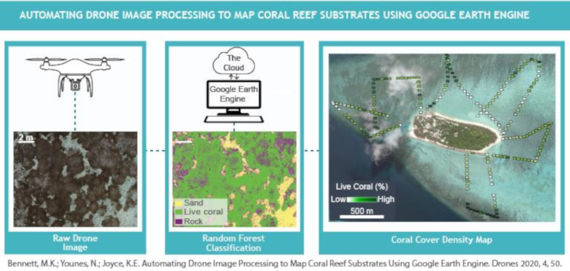
:While coral reef ecosystems hold immense biological, ecological, and economic value, frequent anthropogenic and environmental disturbances have caused these ecosystems to decline globally. Current coral reef monitoring methods include in situ surveys and analyzing remotely sensed data from satellites. However, in situ methods are often expensive and inconsistent in terms of time and space. High-resolution satellite imagery can also be expensive to acquire and subject to environmental conditions that conceal target features. High-resolution imagery gathered from remotely piloted aircraft systems (RPAS or drones) is an inexpensive alternative; however, processing drone imagery for analysis is time-consuming and complex. This study presents the first semi-automatic workflow for drone image processing with Google Earth Engine (GEE) and free and open source software (FOSS). With this workflow, we processed 230 drone images of Heron Reef, Australia and classified coral, sand, and rock/dead coral substrates with the Random Forest classifier. Our classification achieved an overall accuracy of 86% and mapped live coral cover with 92% accuracy. The presented methods enable efficient processing of drone imagery of any environment and can be useful when processing drone imagery for calibrating and validating satellite imagery.

1. Introduction
When the Great Barrier Reef Marine Park Authority released its 2019 Outlook Report, the Authority reported the greatest threat to the Great Barrier Reef was climate change [1]. Dynamical and statistical models and projections demonstrate that climate change is likely to increase the intensity of extreme weather events including tropical cyclones [2], contribute to sea level rise, and increase sea surface temperatures [3]. Each of these aspects pose significant challenges for coral reef environments, and the increasing frequency of mass bleaching events brought on by warmer water temperatures alone threatens the resiliency and survival of reefs worldwide [4,5]. As coral reefs hold immense biological, ecological, and economic value in the services they provide [6], there is a need for cost-effective and efficient practices to map, monitor, and manage coral reef habitats.
Over the last two decades, technological advances have made remote sensing a cost-effective approach when compared to other monitoring methods. Coral reef monitoring programs frequently use in situ field surveys, but they are expensive and often inconsistent in terms of time, space, and scale [7]. These surveys are also limited to areas easily accessible by boat. Remotely sensed imagery collected by satellites and airborne platforms can be used in combination with in situ data to address inconsistencies and enable a higher frequency of consistent observations to effectively observe spatial and temporal changes across reefs [8,9]. To date, multiple characteristics of coral reefs including benthic composition [10], habitat complexity [11], and coral reef state [12,13] have been mapped using remotely sensed imagery. While remotely sensed imagery from satellites has increased the capacity to map coral reefs, obstacles in image spatial resolution and frequency of image acquisition still need to be overcome [14].
Broad scale benthic composition maps over entire reefs with Landsat 8 satellite imagery are promising monitoring resources for researchers and managers [15]. However, the pixel size of moderate spatial resolution satellite imagery is a limiting factor when creating accurate substrate classification models [7]. Large pixel sizes result in lower mapping accuracies of dominant benthic cover types in images, where target substrates are smaller than a single pixel [10]. The authors of [16,17] observed mixed levels of accuracy for substrate classifications due to the inability of the method to differentiate the spatial heterogeneity of reef substrates from the spectral information within pixels. This limitation highlights the need to incorporate higher-resolution imagery in substrate classification models as smaller pixel sizes increase classification accuracies.
High-resolution satellite imagery (i.e., pixel size < 10 m) from Ikonos, WorldView-2, and Quickbird enable higher accuracy when classifying benthic cover types over finer spatial scales [16]. However, these commercially sourced images are expensive to acquire. In general, satellite imagery is also subject to environmental conditions such as cloud cover, sun glint, tidal height, and surface roughness that can obscure or conceal target features. These factors hinder spatial analyses as target features in imagery can be masked and unidentifiable [18,19]. The portable nature of drone platforms enables managers to reduce the influence of these conditions on imagery by capturing data with flexible timing.
Imagery acquired by drones offers several other advantages over satellite imagery. Technological advances increasing battery life, decreases in payload, and decreasing costs make drones a low-cost, valuable resource for marine monitoring over fine spatial scales [20]. The portable nature of drones not only facilitates image acquisition during prime environmental conditions determined by the user, but also at finer temporal resolution than satellites can provide. Unlike drones, revisit times of satellites are not user controlled [21] and multiple drone flights can be made in a single day. Lastly, drones capture imagery at higher spatial resolutions (down to centimeters) when compared to spaceborne platforms, facilitating mapping at greater descriptive resolutions [18], which may lead to more accurate benthic classifications.
Many studies demonstrate the usefulness of drones in terms of marine benthic mapping [13,22,23]. High-resolution drone imagery allows for mapping of seagrass meadows and other habitat types in great detail [22,23]. Information on coral reef state and health can be derived from drones with RGB cameras [13]. However, using drones to create benthic maps of coral reefs is in its infancy [24], and current methods of image analysis are complex and difficult to reproduce [25]. This is because widely used commercial software to analyze drone imagery are not easily accessible to scientists and managers as they often require expensive subscriptions, specialized knowledge, and capable computing hardware to perform analyses on large image collections [26]. Therefore, despite the drone platforms themselves being cheap, readily available, and easily accessible, analyzing their data is not necessarily as simple.
Cloud based infrastructures such as Google Earth Engine (GEE) mitigate the issues identified above by providing sharable, user-friendly platforms to perform sophisticated spatial analysis. GEE promotes user created and training algorithm and classifiers [27], supplies wide collections of available satellite datasets, and uses Google Cloud resources for processing. This increases the ability of researchers to process large datasets using well-known, and cutting-edge algorithms [28]. Using GEE for environmental monitoring has increased since its development in 2010 [29] and several studies use GEE for satellite imagery analysis of terrestrial systems [30,31,32]. However, only a few examples in the peer-reviewed literature use GEE in the marine realm [33,34,35] and these studies have exclusively used satellite imagery. As drone usage is on the rise and more researchers turn to cloud-based platforms for image analysis, we need to create drone imagery analysis workflows that are easily distributable and reproducible.
The objective of this study is to present a distributable, semi-automated workflow using GEE to classify coral reef substrates in drone imagery. We present the steps for drone image pre-processing, substrate classification, and classification accuracy assessment using GEE and free and open source software (FOSS).
2. Methods
2.1. Study Site
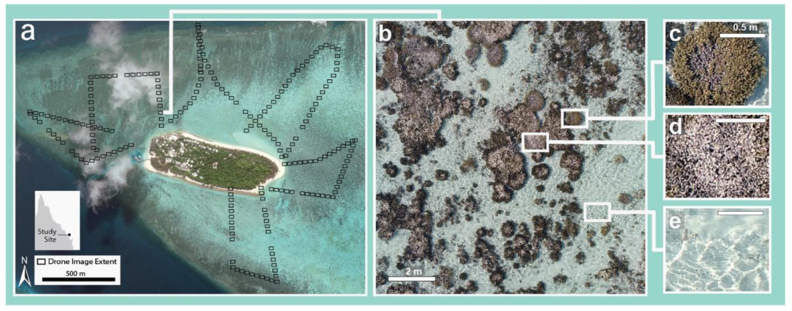
Heron Reef is a coral cay within the Capricorn Bunker Group located near the Tropic of Capricorn in the southern Great Barrier Reef (23.4423°S, 151.9148° E) (Figure 1a). Heron Reef was chosen as the study site because it is a lagoonal platform reef [36] whose shallow reef flats are well suited to effective capture of reef substrate imagery by drone-based cameras. Furthermore, the availability of the University of Queensland Research Station on Heron Island and data from Reef Check Australia’s annual monitoring missions of Heron Reef will enable efficient support for subsequent studies.
2.2. Data Acquisition
True color (RGB) aerial imagery over Heron Reef was collected using a DJI Phantom 4 Pro drone with its camera angled at nadir (FOV = 73.73 deg, pixel array = 5472 × 3648) (Figure 1b). The DJI Phantom 4 Pro was chosen because of its long flight time (~20 minutes), three-axis gimbal that enables smooth flight patterns to capture imagery and 20-megapixel RGB sensor. The drone was oriented south and flown at 20 m altitude resulting in a ground sample distance (GSD) equaling 0.5 cm and individual photo footprints of approximately 20.1 × 16.7 m. The GSD enabled identification of major substrate types for classification (Figure 1c–e). Flight paths were programmed through the Litchi mission planning desktop and mobile application and captured photos every 40 m along the flight paths. Images were collected from 14:30 to 17:00 on February 20, 2019, to coincide with low tide and reduce the effects of sun glint and surface roughness. Depths of the study area during low tide ranged from exposed coral to 40 cm of depth. After data collection, it was evident the drone camera failed to take photos at some points along the flight path (Figure 1a). However, the large sample size of drone imagery collected (n = 230) still enabled a thorough representation and assessment of the selected substrates on Heron Reef.
Drone flight paths are usually designed following the standard aerial survey pattern, where the drone flies up and down adjacent flight paths to create a geometric area of coverage. However, we decided not to use this flight pattern. We programmed the drone path as shown in Figure 1a for two main reasons: (1) to cover a greater variety of habitats in more areas around Heron Reef and (2) for later use to calibrate and validate satellite imagery of Heron Reef.
2.3. Data Processing
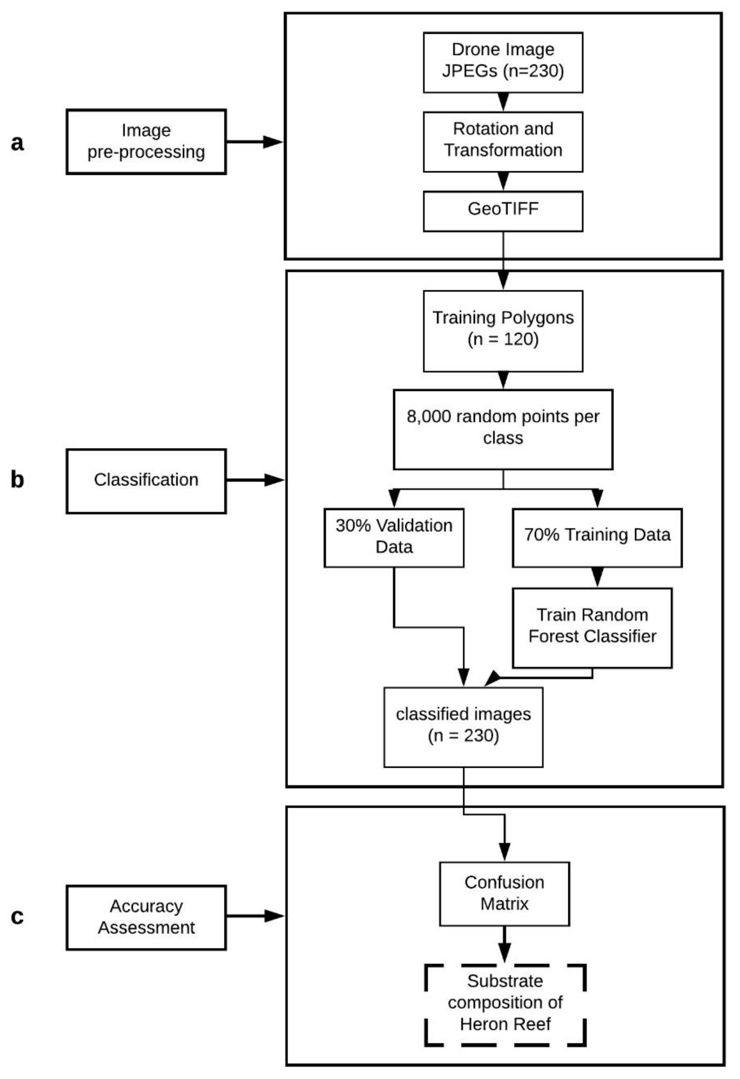
We divided the workflow in this study into three phases: (a) drone image pre-processing, (b) image classification, (c) accuracy assessment (Figure 2).
2.4. Image Pre-Processing
Google Earth Engine currently requires imagery to be in a GeoTIFF format before it can be ingested into the system. Drone images were therefore converted from their native JPEG format to GeoTIFF files using the Python programming language (Figure 2a). First, images were rotated 180° to the left for correct orientation. Latitude and longitude co-ordinates were extracted from each image through ExifTool, a free and open source software program for editing image, audio, video, and PDF metadata. These co-ordinates were then converted into Easting and Northing values (EPSG: 32,756 [WGS 84/UTM zone 56S]) in QGIS. Image rasters were also projected to EPSG: 32,756 in QGIS. TIFF word files (TFW) were created for each TIFF. They are plain text files that store X and Y pixel size, image rotational information, and co-ordinates for images stored as TIFF files. TFW header files created for each GeoTIFF recognize the Easting and Northing values as the upper left corner of the images instead of the image centers, which is where the images are typically tagged. Therefore, to ensure images were in the correct locations, 12.5541 m (half the image width) was subtracted from each Easting value and 8.3694 m (half of the image height) was subtracted from each Northing value.
2.5. Image Classification
After pre-processing, all drone images of Heron Reef were uploaded as an image collection asset in GEE (Figure 2b). We chose rock/dead coral, sand, and live coral for substrate classification, as these substrates were most easily recognizable in the drone imagery. It should be noted that the rock/dead coral class includes epilithic algae matrix and dead hard coral. We also created a sun glint class to account for the impacts of sun glint classifying substrates and subsequently determining their areal coverage.
The GSD of the drone images enables visual identification of major substrate types, which is acceptable to use as reference data for training the classifier and accuracy assessment [37]. Traditional methods of collecting in situ data for calibrating and validating satellite data [38] have positional accuracies far lower than the scale of drone observation, particularly when attempting to co-register with drone imagery that also has its own positional inaccuracy. Areas that best represent each class were visually identified in the drone imagery in GEE. We then used the geometry tool to manually create 30 representative polygons per class (n = 120) (Figure 3a).
To ensure an even sampling of training and validation pixels across the classes, we selected 8000 random points (pixels) per class (n = 32,000 points) from within the training polygons. We merged these points into a feature collection to be mapped across the images to extract digital number statistics for each category. We then split the points into 70% training and 30% validation data.
We employed the Random Forest algorithm with 50 trees for classification in GEE (Figure 3b). Preliminary tests to fine tune the classifier concluded 50 trees as the optimum number of trees to use, as this resulted in the highest training accuracy (90%) and lowest out of bag error (14%). The Random Forest classifier is not sensitive to noise or outliers and has been used with high accuracy to map benthic habitats of coral reefs [39] and tidal flats [40]. This classifier was applied to the image collection, and the total area (m2) per substrate per drone image was calculated to create substrate cover maps.
2.6. Accuracy Assessment
An accuracy assessment was employed to assess the accuracy of the final classification result over the entire image collection of drone imagery (Figure 2c). Validation points (n = 9522 from the 30% validation data) were applied over the classification result to extract pixel classification information at each point. An error matrix was generated to compare how the classifier classified the validation points with our reference classification. The error matrix was used to compute the overall accuracy of the classification by dividing the total number of correctly classified pixels by the total number of reference pixels sampled. Producer and user accuracy metrics were calculated by class. Producer accuracy (precision) was calculated by dividing the number of correctly classified pixels in a class by the total number of reference pixels sampled for that class. This displays how well the classifier identified classes in the training data set [41]. User accuracy (recall) was computed by taking the total number of correctly classified pixels for a class and dividing it by the total number of pixels classified as that class by the algorithm. User accuracy represents the chance that the class classified on the map represents that class in the field [41].
2.7. Code and Data Access
The code for image pre-processing, classification (including additional parameters set for Random Forest), and accuracy assessment is available online, as both a live version (https://github.com/bennkat/Drone_Image_Processing_GEE/tree/v1.0) and a static release as per this paper (https://0-doi-org.brum.beds.ac.uk/10.5281/zenodo.3986067).
3. Results
3.1. Image Classification
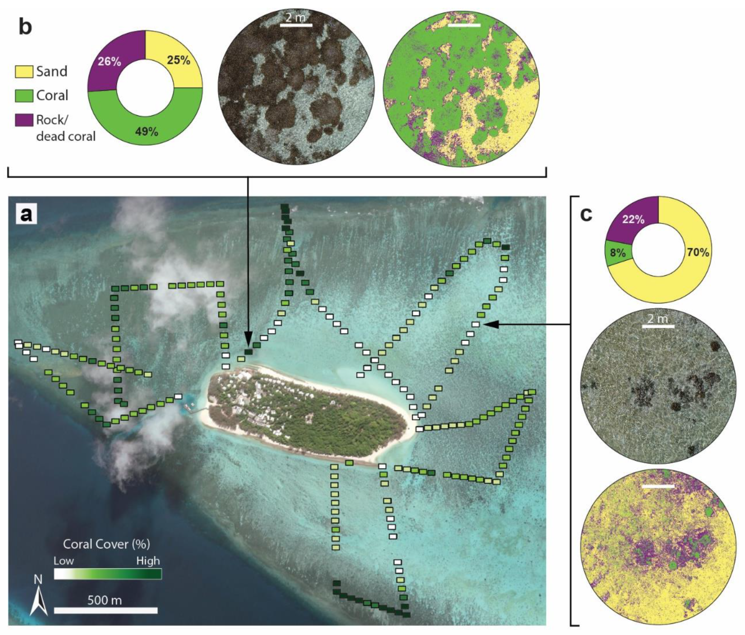
Using our semi-automated workflow, we classified 230 drone images of Heron Reef, representing a total area of 96,664 m2. A visual assessment of the classification results revealed that this workflow is able to distinguish between live coral, rock/dead coral, and sand substrates present in drone imagery (Figure 4). Our workflow classified a total area of 15,240 m2 of Heron Reef as live coral, 23,795 m2 as sand, and 38,148 m2 as rock/dead coral substrate. Predicted live coral cover percentages of Heron Reef range from less than 1% to 60% (Figure 4a). The highest estimated coral cover was observed along the reef slope and the lowest coral cover observed in reef flats (Figure 4b,c).
3.2. Accuracy Assessment
Comparison of validation pixels with substrate class assignments made by the model, showed an overall mapping accuracy of 86%. Accuracy calculations and the error matrix (Table 1 and Table 2) demonstrate differences between the model classification and substrate classes assigned manually. The producer and user accuracies for live coral indicate that Random Forest classified 92% of reference live coral pixels correctly and correctly classifies live coral in unseen data 86% of the time (Table 1). The model also displayed high accuracy in mapping sand (Table 1). The rock/dead coral class displayed the lowest mapping accuracy with an accuracy of 71% (Table 1). This accuracy results from the misclassification of rock/dead coral as live coral. While the model was able to classify 92% of the live coral reference pixels correctly, it classified 14% of the rock/dead coral reference pixels as live coral, leading the model to overpredict live coral cover (Table 2).
After visual inspection of the classification result, the model was unable to differentiate spectral information between rock/dead coral, sand, and sun glint classes in some areas around Heron Reef. Within our classification, seven percent of sand and eight percent of rock/dead coral reference pixels were classified as sun glint (Table 2). Additionally, 11% of the drone images had greater than 40% of the image area classified as sun glint, therefore excluding actual rock/dead coral, sand, and live coral assignments. However, the model successfully distinguished sun glint from the live coral class, with less than one percent of sun glint reference pixels classified as live coral (Table 2).
4. Discussion
4.1. Image Classification Accuracy
We produced a substrate classification of Heron Reef, Australia, with an overall mapping accuracy of 86%, which maps coral cover with 92% accuracy. Coral cover substrate percentages produced from this classification workflow are within substrate cover ranges for Heron Reef published by Reef Check Australia (RCA) in 2018. The Reef Check Australia 2018 Heron Island Reef Health Report reported an average of 42% hard coral cover observed across 15 monitoring sites, with coverage ranging from absent to 73% [42]. The greatest coral coverage was observed in reef slope habitats, with less coral coverage found amongst sandy reef flats. These spatial patterns of coral cover published in the Reef Check Australia 2018 Heron Island Reef Health Report were also observed within our classification result. Discrepancies between the estimated coral coverage found from our study and the coral coverage observed by RCA could be attributed to monitoring site location. Out of eight reef slope sites monitored by RCA, three sites showed greater than 70% hard coral cover. The other five sites ranged from 53% to 67%. Our drone imagery may have overlapped portions of the reef slope that exhibited coral cover with in the 53–67% range, therefore not matching the highest coverage percentages observed by RCA. We recognize that areas of Heron Reef may exhibit higher coral coverage than estimated in this study, but those areas may have not been represented in our drone imagery.
The presented methods provide steps for image preprocessing, so drone imagery is formatted for other classification techniques and algorithms in GEE that can be used to classify coral cover. Since the appropriateness of a classifier is dependent on the characteristics of the dataset being classified, users who want to implement this workflow can test the accuracies of other algorithms on their data and decide which one is best suited to provide the most accurate classification results. GEE offers tools for Object-Based Image Analysis (OBIA) techniques, which have been used to map coral cover in satellite imagery with resolutions of 2–30 m [35,43]. However, the authors of [43] also incorporated bathymetry data to develop segmentation rules for classification. As live corals exist in a variety of shapes, textures, and sizes in drone imagery, users may need to include additional datasets such as bathymetry to successfully apply OBIA to this workflow. Other classification algorithms such as support vector machine, and classification and regression trees are also available in GEE and can be used to classify coral reef habitats [39].
While the algorithm used will impact classification accuracy, environmental conditions such as sun glint can obscure classification targets and thus affect the final result [44]. Although steps were taken to minimize the presence of sun glint in the imagery used in this study, sun glint that was present in the images had to be accounted for. The creation of a sun glint class resulted in slight inaccuracies as the classifier misclassified sun glint, rock/dead coral, and sand substrates. Currently, GEE offers masking functions for atmospheric corrections of satellite data [29] and sun glint correction algorithms have been developed and used on high-resolution imagery of marine environments outside of the GEE platform [45]. However, these algorithms use near infrared (NIR) bands to identify sun glint affected pixels. As the imagery for this study was collected with a consumer-grade RGB camera, these sun glint correction algorithms would not be applicable. An alternative solution for future iterations of this workflow includes applying a mask that filters for pixels close to saturation (RGB = 255, 255, 255) or include a subset from within a spatially defined window of the image during image preprocessing. This would remove sun glint from the imagery and may decrease misclassifications between sun glint, rock/dead coral, and sand classes.
Other environmental factors like water quality, wind, and sea state, that create ripples or waves and differ in extent on other coral reefs, may impact drone image quality [19,46] and hinder substrate classifications. These factors should be considered during flight planning, and steps should be taken to mitigate the impacts of these factors on imagery, if possible. Completing flight missions during low tide and optimum weather conditions with low wind would reduce effects of ripples and waves on obscuring target features. However, shallow reef environments are optimal for aerial mapping [19].
Combining spectral information procured from optical sensors with bathymetric data can make this workflow applicable to other coral reef ecosystems with varying depths. In this study, depth is not a limiting factor, as drone imagery was collected over the reef flat at low tide to minimize the impacts of water depth on classification results. As spectral reflectance of substrates becomes more similar with increasing depth [7,14], combining bathymetric data with spectral information may increase the applicability of this workflow. The authors of [47] observed the greatest overall mapping accuracies in supervised and unsupervised benthic classifications (71% and 70%, respectively) of Glover’s Atoll, Belize, after combining layers of acoustic roughness, hardness, and depth, with depth corrected optical layers from IKONOS imagery. The authors of [47] do note a limitation with the extensive field surveys required to calibrate acoustic data on an image by image basis. Furthermore, acoustic data can only be acquired in areas accessible by boat [18]. Bathymetric data acquired through light detection and ranging (LiDAR) sensors mounted on drones can overcome these limitations. Datasets from such methods have been used in combination with RGB drone imagery to assess coral reef bathymetry and have the potential to aid coral reef benthic classifications [48].
Assessing the accuracy of thematic maps is essential as it informs users on the reliability of the map product and impacts what the map can be used for. However, recommended and widely used techniques of assessment, such as comparing classification results to ground-truthing data through a confusion matrix, pose many challenges [49]. Issues with scale [50], site accessibility, and funding [7] often result in ground-truthing data that might not be available or suitable to use. Field data was available for ground-truthing assessment in this study but could not be used due to scale issues and potential GPS location errors, which would not allow for direct comparisons to classifications of sub centimeter pixels. Future field data acquisition campaigns for calibrating and validating classifications of drone imagery include georeferenced quadrat sampling [23,51] in combination with underwater imagery of substrate, to reduce GPS location errors. In lieu of comparisons with field data, accuracy assessments that use the same initial source information for reference and validation data have proven a credible alternative [52]. These accuracy assessments also avoid errors that result from the mislocation of reference data and points in the classification result [53].
As the classification of substrates for training data in this study was completed manually, over and under-estimates of substrate cover percentages may also be the result of misidentification of classes due to human error when training polygons were created during the training stage. The current spatial resolution of the GEE base map (where the scale bar equals 2 m) prevents observing drone imagery at native resolution. Since mislabeling of classes by the interpreter during classifier training can decrease the accuracy of map products [54], efforts were taken to minimize substrate misinterpretation. Live coral, rock/dead coral, and sand substrates were chosen because they were the most easily identifiable substrates. As a result, the classifier classified substrates such as algae and rubble under the classes chosen, affecting classification accuracy. Since the main goal was to automate a workflow with FOSS to enable mapping of coral reef substrates in drone imagery, the number of substrate classes used was enough to achieve this goal.
4.2. Workflow Assessment
We created a straightforward and efficient semi-automatic workflow that processes drone imagery for analysis and uses the Random Forest algorithm for benthic mapping of reef ecosystems. Steps for image pre-processing were created by the authors. Prior to this workflow, coding examples in GEE and published research that classified imagery using GEE use satellite imagery. The presented image classification steps consist of code previously used for classifying satellite imagery but have been modified and adapted for drone imagery collections. The accuracy assessment phase uses previously established code in GEE for accuracy assessment but is modified for this study’s data. Our workflow pieces together image processing with image classification in GEE to make classifications of drone imagery with greater descriptive resolutions than satellite imagery possible. While drone imagery has been used to evaluate benthic characteristics of marine environments [13,22,23], this is the first study to present a semi-automatic process that formats and classifies drone imagery to map coral reef substrates using FOSS and GEE.
The semi-automation of drone imagery pre-processing, substrate classification, and accuracy assessment phases makes drone imagery analysis more widely available and reproducible. Datasets acquired from drones are often informationally dense [18] and require complicated processing. This workflow demonstrates straightforward image processing steps that can be applied to any drone acquired image collection. Furthermore, FOSS enables drone imagery analysis to users and organizations who lack the resources to pay for licenses of commercial products. Anyone with an internet connection and a computer can apply this workflow to their own drone imagery and share their code and datasets. This is a significant advancement, as reproducibility in remote sensing studies, especially regarding classification calibration and validation, is an obstacle [37,55].
The main limitation of this workflow is the number of programs used to convert drone images into GeoTIFF files. While these programs are FOSS, further automating this phase through Jupyter notebook and Python API for GEE would reduce the amount of time and effort needed for image preprocessing as well as the total amount of time needed for image classification and analysis.
5. Future Applications
This study presents a tool that can be used to process drone imagery of any environment for image classification and analysis. Drones and consumer grade cameras are used to monitor land use/cover [56], survey forest canopies, biodiversity, and assess deforestation [57,58], as well as map mangrove forests [59]. Lengthy processing times in addition to the processing power needed to analyze high-resolution imagery are common obstacles that often detract from time savings and effort gained by using drones to collect field data [60,61]. The presented methods drastically reduce image processing time through FOSS to enable analysis of drone imagery of any ecosystem, not only coral reefs.
Other applications include using this workflow to process drone imagery to calibrate and validate satellite imagery and establish baselines for temporal variation. Monitoring coral reefs from Earth observation data address many of the shortcomings of current in situ monitoring programs [7]. Imagery from drones can work collaboratively with in situ data to more accurately inform calibrations and validations of satellite imagery. Imagery from drones is proving to be highly effective in training and validating classifications made by satellite imagery [61] and studies note the usability of their drone derived datasets for calibrating satellite imagery [48]. This workflow provides accessible methods for rapid drone image processing to enable use of drone imagery as first-order ground truthing for satellite data. Additionally, imagery from drones can be used to evaluate temporal variation on coral reefs [62]. Effective ecosystem assessment and monitoring is dependent on the ability to monitor area changes over time. This workflow can provide more descriptive spatial layers to projects like the Allen Coral Atlas Project (in addition to using this workflow to calibrate and validate satellite data) [35]. Furthermore, using this workflow to process remotely sensed data to monitor shallow reef flats and crests will benefit existing monitoring programs, like the Australian Institute of Marine Science Long-term Monitoring Program and Marine Monitoring Program, that focus on reef depths greater than 2 m.
6. Conclusions
Although the use of remotely sensed imagery from drones for ecosystem monitoring has increased, methods for drone imagery processing are still time consuming and complex. This is the first study to present a widely accessible and reproducible semi-automatic workflow that enables rapid processing of drone imagery for image analysis using FOSS and GEE. Under this workflow, we processed and classified 230 drone images of Heron Reef, Australia and produced a substrate classification with an overall accuracy of 86%, which mapped coral cover with 92% accuracy. The accessible and reproducible nature of this workflow opens drone image processing and assessment to anyone with an internet connection. Drone imagery of any environment, marine or terrestrial, can be processed, classified, and assessed for accuracy. Further applications of this methodology include processing drone imagery for the purpose of calibrating and validating satellite imagery. This study provides cheap and efficient methods to process and assess drone imagery that will benefit monitoring efforts worldwide.
Author Contributions
Conceptualization, M.K.B. and K.J.; methodology, M.K.B., N.Y., and K.J.; data collection: M.K.B. and K.J.; formal analysis: M.K.B.; original draft preparation, M.K.B.; review and editing, M.K.B., N.Y., and K.J. All authors have read and agreed to the published version of the manuscript.
Funding
There was no external funding provided for this project.
Acknowledgments
We would like to thank Stephanie Duce for her help in collecting drone imagery. We acknowledge useful assessments and correction from four anonymous reviewers as well as the journal editor.
Conflicts of Interest
The authors declare no conflict of interest.
References
- GBRMPA. Great Barrier Reef Outlook Report 2019; Great Barrier Reef Marine Park Authority: Townsville, Australia, 2019.
- Knutson, T.; Camargo, S.J.; Chan, J.C.; Emanuel, K.; Ho, C.H.; Kossin, J.; Mohapatra, M.; Satoh, M.; Sugi, M.; Walsh, K.; et al. Tropical cyclones and climate change assessment: Part II: Projected response to anthropogenic warming. Bull. Am. Meteorol. Soc. 2020, 101, E303–E322. [Google Scholar] [CrossRef]
- Boko, M.; Niang, I.; Nyong, A.; Vogel, A.; Githeko, A.; Medany, M.; Osman-Elasha, B.; Tabo, R.; Yanda, P.Z. Intergovernmental Panel on Climate Change. Sea Level Change. In Climate Change 2013—The Physical Science Basis: Working Group I Contribution to the Fifth Assessment Report of the Intergovernmental Panel on Climate Change; Cambridge University Press: Cambridge, UK, 2014; pp. 1137–1216. [Google Scholar]
- Hughes, T.P.; Kerry, J.T.; Álvarez-Romero, M.J.; Álvarez-Romero, G.; Anderson, K.D. Global warming and recurrent mass bleaching of corals. Nature 2017, 543, 373–377. [Google Scholar] [CrossRef] [PubMed]
- Harrison, H.B.; Álvarez-Noriega, M.; Baird, A.H.; Heron, S.F.; MacDonald, C.; Hughes, T.P. Back-to-back coral bleaching events on isolated atolls in the Coral Sea. Coral Reefs 2019, 38, 713–719. [Google Scholar] [CrossRef]
- Barbier, E.B.; Hacker, S.D.; Kennedy, C.; Koch, E.W.; Stier, A.C.; Silliman, B.R. The value of estuarine and coastal ecosystem services. Ecol. Monogr. 2011, 81, 169–193. [Google Scholar] [CrossRef]
- Hedley, J.D.; Roelfsema, C.M.; Chollett, L.; Harborne, A.R.; Heron, S.F.; Weeks, S.; Skirving, W.J.; Strong, A.E.; Eakin, C.M.; Christensen, T.R.L.; et al. Remote sensing of coral reefs for monitoring and management: A review. Remote. Sens. 2016, 8, 118. [Google Scholar] [CrossRef] [Green Version]
- Mumby, P.J.; Skirving, W.; Strong, A.E.; Hardy, J.T.; LeDrew, E.L.; Hochberg, E.J.; Stumpf, R.P.; David, L.P. Remote sensing of coral reefs and their physical environment. Mar. Pollut. Bull. 2004, 48, 219–228. [Google Scholar] [CrossRef]
- Goodman, J.A.; Purkis, S.J.; Phinn, S.R. Coral Reed Remote Sensing A Guide for Mapping, Monitoring and Managemen; Springer: Berlin/Heidelberg, Germany, 2013. [Google Scholar]
- Roelfsema, C.; Kovacs, E.; Carlos Ortiz, J.; Wolff, N.H.; Callaghan, D.; Wettle, M.; Ronan, M.; Hamylton, S.M.; Mumby, P.J.; Phinn, S. Coral reef habitat mapping: A combination of object-based image analysis and ecological modelling. Remote. Sens. Environ. 2018, 208, 27–41. [Google Scholar] [CrossRef]
- Storlazzi, C.D.; Dartnell, P.; Hatcher, G.A.; Gibbs, A.E. End of the chain? Rugosity and fine-scale bathymetry from existing underwater digital imagery using structure-from-motion (SfM) technology. Coral Reefs 2016, 35, 889–894. [Google Scholar] [CrossRef]
- Collin, A.; Planes, S. Enhancing coral health detection using spectral diversity indices from worldview-2 imagery and machine learners. Remote. Sens. 2012, 4, 3244–3264. [Google Scholar] [CrossRef] [Green Version]
- Collin, A.; Ramambason, C.; Pastol, Y.; Casella, E.; Rovere, A.; Thiault, L.; Espiau, B.; Siu, G.; Lerouvreur, F.; Nakamura, N.; et al. Very high resolution mapping of coral reef state using airborne bathymetric LiDAR surface-intensity and drone imagery. Int. J. Remote. Sens. 2018, 39, 5676–5688. [Google Scholar] [CrossRef] [Green Version]
- Purkis, S.J. Remote sensing tropical coral reefs: The view from above. Annu. Rev. Mar. Sci. 2018, 10, 149–168. [Google Scholar] [CrossRef] [PubMed]
- Haya, Y.L.O.M.; Fuji, M. Mapping the change of coral reefs using remote sensing and in situ measurements: A case study in Pangkajene and Kepulauan Regency, Spermonde Archipelago, Indonesia. J. Oceanogr. 2017, 73, 623–645. [Google Scholar] [CrossRef]
- Saul, S.; Perkis, S. Semi-automated object-based classification of coral reef habitat using discrete choice models. Remote. Sens. 2015, 7, 15894–15916. [Google Scholar] [CrossRef] [Green Version]
- Collin, A.; Laporte, J.; Koetz, B.; Martin-Lauzer, F.R.; Desnos, Y.L. Mapping bathymetry, habitat, and potential bleaching of coral reefs using Sentinel-2. In Proceedings of the 13th International Coral Reef Symposium, Honolulu, HI, USA, 19–24 June 2016; pp. 405–420, <hal-01460593>. [Google Scholar]
- Hedley, J.D.; Roelfsema, C.M.; Phinn, S.R.; Mumby, P.J. Environmental and sensor limitations in optical remote sensing of coral reefs: Implications for monitoring and sensor design. Remote. Sens. 2012, 4, 271–302. [Google Scholar] [CrossRef] [Green Version]
- Joyce, K.E.; Duce, S.; Leahy, S.M.; Leon, J.; Maier, S.W. Principles and practice of acquiring drone-based image data in marine environments. Mar. Freshw. Res. 2019, 70, 952–963. [Google Scholar] [CrossRef]
- Colefax, A.P.; Butcher, P.A.; Kelaher, B.P. The potential for unmanned aerial vehicles (UAVs) to conduct marine fauna surveys in place of manned aircraft. ICES J. Mar. Sci. 2017, 75, 1–8. [Google Scholar] [CrossRef]
- Fernández-Guisuraga, J.M.; Sanz-Ablanedo, E.; Suárez-Seoane, S.; Calvo, L. Using unmanned aerial vehicles in postfire vegetation survey campaigns through large and Heterogeneous Areas: Opportunities and challenges. Sensors 2018, 18, 856. [Google Scholar] [CrossRef] [Green Version]
- Topouzelis, K.; Papakonstantinou, A.; Doukari, M.; Stamatis, P.; Makri, D.; Katsanevakis, S. Coastal habitat mapping in the Aegean Sea using high resolution orthophoto maps. In Proceedings of the Fifth International Conference on Remote Sensing and Geoinformation of the Environment, Paphos, Cyprus, 20–23 March 2017; International Society for Optics and Photonics: Bellingham, WA, USA, 2017; Volume 10444, p. 1044417. [Google Scholar]
- Duffy, J.P.; Pratt, L.; Anderson, K.; Land, P.E.; Shutler, J.D. Spatial assessment of intertidal seagrass meadows using optical imaging systems and a lightweight drone. Estuar. Coast. Shelf Sci. 2018, 200, 169–180. [Google Scholar] [CrossRef]
- Ventura, D.; Bonifazi, A.; Gravina, M.F.; Belluscio, A.; Ardizzone, G. Mapping and classification of ecologically sensitive marine habitats using unmanned aerial vehicle (UAV) imagery and object-based image analysis (OBIA). Remote. Sens. 2018, 10, 1331. [Google Scholar] [CrossRef] [Green Version]
- Morales-Barquero, L.; Lyons, M.B.; Phinn, S.R.; Roelfsema, C.M. Trends in remote sensing accuracy assessment approaches in the context of natural resources. Remote. Sens. 2019, 11, 2305. [Google Scholar] [CrossRef] [Green Version]
- Alonso, A.; Muñoz-Carpena, R.; Kennedy, R.E.; Murcia, C. Wetland landscape spatio-temporal degradation dynamics using the new google earth engine cloud-based platform: Opportunities for non-specialists in remote sensing. Trans. ASABE 2016, 59, 1333–1344. [Google Scholar]
- Gorelick, N.; Hancher, M.; Dixon, M.; Ilyushchenko, S.; Thau, D.; Moore, R. Google Earth Engine: Planetary-scale geospatial analysis for everyone. Remote. Sens. Environ. 2017, 202, 18–27. [Google Scholar] [CrossRef]
- Kumar, L.; Mutanga, O. Google Earth Engine applications. Remote. Sens. 2019, 11, 420. [Google Scholar]
- Kumar, L.; Mutanga, O. Google Earth Engine applications since inception: Usage, trends, and potential. Remote. Sens. 2018, 10, 1509. [Google Scholar] [CrossRef] [Green Version]
- Robinson, N.P.; Allred, B.W.; Jones, M.O.; Moreno, A.; Kimball, J.S.A. Dynamic Landsat derived normalized difference vegetation index (NDVI) product for the conterminous United States. Remote. Sens. 2017, 9, 863. [Google Scholar] [CrossRef] [Green Version]
- He, M.; Kimball, J.S.; Maneta, M.P.; Maxwell, B.D.; Moreno, A.; Beguería, S.; Wu, X. Regional crop gross primary productivity and yield estimation using fused landsat-MODIS data. Remote. Sens. 2018, 10, 372. [Google Scholar] [CrossRef] [Green Version]
- Tsai, Y.; Stow, D.; Chen, H.; Lewison, R.; An, L.; Shi, L. Mapping vegetation and land use types in fanjingshan national nature reserve using Google Earth Engine. Remote. Sens. 2018, 10, 927. [Google Scholar] [CrossRef] [Green Version]
- Traganos, D.; Aggarwal, B.; Poursanidis, D.; Topouzelis, K.; Chrysoulakis, N.; Reinartz, P. Towards global-scale seagrass mapping and monitoring using Sentinel-2 on Google Earth Engine: The case study of the aegean and ionian seas. Remote. Sens. 2018, 10, 1227. [Google Scholar] [CrossRef] [Green Version]
- Sagawa, T.; Yamashita, Y.; Okumura, T.; Yamanokuchi, T. Satellite derived bathymetry using machine learning and multi-temporal satellite images. Remote. Sens. 2019, 11, 1155. [Google Scholar] [CrossRef] [Green Version]
- Lyons, B.M.; Roelfsema, C.M.; Kennedy, E.V.; Kovacs, E.M.; Borrego-Acevedo, R.; Markey, K.; Roe, M.; Yuwono, D.M.; Harris, D.L.; Phinn, S.R.; et al. Mapping the world’s coral reefs using a global multiscale earth observation framework. Remote. Sens. Ecol. Conversat. 2020, 1–12. [Google Scholar] [CrossRef] [Green Version]
- Jell, J.S.; Flood, P.G. Guide to the Geology of Reefs of the Capricorn and Bunker Groups, Great Barrier Reef Province, with Special Reference to Heron Reef; University of Queensland Press: Brisbane, Australia, 1978; Volume 8, p. 85. [Google Scholar]
- Congalton, R.G. Accuracy assessment and validation of remotely sensed and other spatial information. Int. J. Wildland Fire 2001, 10, 321–328. [Google Scholar] [CrossRef] [Green Version]
- Roelfsema, C.M.; Phinn, S.R. Integrating field data with high spatial resolution multispectral satellite imagery for calibration and validation of coral reef benthic community maps. J. Appl. Remote Sens. 2010, 4, 043527. [Google Scholar] [CrossRef] [Green Version]
- Wicaksono, P.; Aryaguna, P.A.; Lazuardi, W. Benthic habitat mapping model and cross validation using machine-learning classification algorithms. Remote. Sens. 2019, 11, 1279. [Google Scholar] [CrossRef] [Green Version]
- Murray, N.J.; Phinn, S.R.; DeWitt, M.; Ferrari, R.; Johnston, R. The global distribution and trajectory of tidal flats. Nature 2019, 565, 222–225. [Google Scholar] [CrossRef]
- Granshaw, S. Fundamentals of satellite remote sensing: An environmental approach. Photogramm. Rec. 2017, 32, 61–62. [Google Scholar] [CrossRef]
- Salmond, J.; Passenger, J.; Kovaks, E.; Roelfsema, C.; Stetner, D. Reef Check Australia 2018 Heron Island Reef Health Report; Reef Check Foundation Ltd.: Marina del Rey, CA, USA, 2018. [Google Scholar]
- Phinn, S.R.; Roelfsema, C.M.; Mumby, P.J. Multi-scale, object-based image analysis for mapping geomorphic and ecological zones on coral reefs. Int. J. Remote Sens. 2011, 33, 3768–3797. [Google Scholar] [CrossRef]
- Doukari, M.; Batsaris, M.; Papakonstantinou, A.; Topouzelis, K. A Protocol for aerial survey in coastal Areas using UAS. Remote. Sens. 2019, 11, 1913. [Google Scholar] [CrossRef] [Green Version]
- Traganos, D.; Poursanidis, D.; Aggarwal, B.; Chrysoulakis, N.; Reinartz, P. Estimating satellite-derived bathymetry (SDB) with the google earth engine and sentinel-2. Remote. Sens. 2018, 10, 859. [Google Scholar] [CrossRef] [Green Version]
- Mount, R. Acquisition of through-water aerial survey images: Surface effects and the prediction of sun glitter and subsurface illumination. Photogramm. Eng. Remote. Sens. 2005, 71, 1407–1415. [Google Scholar] [CrossRef]
- Bejarano, S.; Mumby, P.J.; Hedley, J.D.; Sotheran, I. Combining optical and acoustic data to enhance the detection of Caribbean forereef habitats. Remote. Sens. Environ. 2010, 114, 2768–2778. [Google Scholar] [CrossRef]
- Casella, E.; Collin, A.; Harris, D.; Ferse, S.; Bejarano, S.; Parravicini, V.; Hench, J.L.; Rovere, A. Mapping coral reefs using consumer-grade drones and structure from motion photogrammetry techniques. Coral Reefs 2017, 36, 269–275. [Google Scholar] [CrossRef]
- Foody, G.M. Status of land cover classification accuracy assessment. Remote. Sens. Environ. 2002, 80, 185–201. [Google Scholar] [CrossRef]
- Wu, H.; Li, Z.L. Scale issues in remote sensing: A review on analysis, processing and modeling. Sensors 2009, 9, 1768–1793. [Google Scholar] [CrossRef] [PubMed]
- Collin, A.; Archambault, P.; Planes, S. Revealing the regime of shallow coral reefs at patch scale by continuous spatial modeling. Front. Mar. Sci. 2014, 1, 65. [Google Scholar] [CrossRef]
- Baraldi, A.; Bruzzone, L.; Blonda, P. Quality assessment of classification and cluster maps without ground truth knowledge. IEEE Trans. Geosci. Remote. Sens. 2005, 43, 857–873. [Google Scholar] [CrossRef]
- Foody, G.M. Harshness in image classification accuracy assessment. Int. J. Remote Sens. 2008, 29, 3137–3158. [Google Scholar] [CrossRef] [Green Version]
- Powell, R.L.; Matzke, N.; de Souza, C., Jr.; Clark, M.; Numata, I.; Hess, L.L.; Roberts, D.A. Sources of error in accuracy assessment of thematic land-cover maps in the Brazilian Amazon. Remote. Sens. Environ. 2004, 90, 221–234. [Google Scholar] [CrossRef]
- Lyons, M.B.; Keith, D.A.; Phinn, S.R.; Mason, T.J.; Elith, J. A comparison of resampling methods for remote sensing classification and accuracy assessment. Remote. Sens. Environ. 2018, 208, 145–153. [Google Scholar] [CrossRef]
- Koh, L.P.; Wich, S.A. Dawn of drone ecology: Low-cost autonomous aerial vehicles for conservation. Trop. Conserv. Sci. 2012, 5, 121–132. [Google Scholar] [CrossRef] [Green Version]
- Getzin, S.; Wiegand, K.; Schöning, I. Assessing biodiversity in forests using very high-resolution images and unmanned aerial vehicles. Methods Ecol. Evol. 2011, 3, 397–404. [Google Scholar] [CrossRef]
- Tang, L.; Shao, G. Drone remote sensing for forestry research and practices. J. For. Res. 2015, 26, 791–797. [Google Scholar] [CrossRef]
- Ruwaimana, M.; Satyanarayana, B.; Otero, V.; Muslim, A.M.; Muhammad, S.A. The advantages of using drones over space-borne imagery in the mapping of mangrove forests. PLoS ONE 2018, 13, e0200288. [Google Scholar] [CrossRef] [PubMed] [Green Version]
- Barnas, A.F.; Darby, B.J.; Vandeberg, G.S.; Rockwell, R.F.; Ellis-Felege, S.N. A comparison of drone imagery and ground-based methods for estimating the extent of habitat destruction by lesser snow geese (Anser caerulescens caerulescens) in La Pérouse Bay. PLoS ONE 2019, 14, e0217049. [Google Scholar] [CrossRef] [Green Version]
- Gray, P.C.; Ridge, J.T.; Poulin, S.K.; Seymour, A.C.; Schwantes, A.M.; Swenson, J.J.; Johnston, D.W. Integrating drone imagery into high resolution satellite remote sensing assessments of estuarine environment. Remote. Sens. 2018, 10, 1257. [Google Scholar] [CrossRef] [Green Version]
- Fallati, L.; Saponari, L.; Savini, A.; Marchese, F.; Corselli, C.; Galli, P. Multi-Temporal UAV Data and object-based image analysis (OBIA) for estimation of substrate changes in a post-bleaching scenario on a maldivian reef. Photogramm. Eng. Remote. Sens. 2020, 12, 2093. [Google Scholar] [CrossRef]
Figure 1.
(a) Heron Reef study site, in the southern Great Barrier Reef, Australia. (b) Drone image with examples showing benthic cover for classification: (c) live coral, (d) rock/dead coral, and (e) sand.
Figure 1.
(a) Heron Reef study site, in the southern Great Barrier Reef, Australia. (b) Drone image with examples showing benthic cover for classification: (c) live coral, (d) rock/dead coral, and (e) sand.

Figure 2.
Workflow using classification and accuracy assessment tools in Google Earth Engine (GEE).

Figure 3.
(a) Drone image in GEE with class polygons. (b) Classification result from Random Forest in GEE.
Figure 3.
(a) Drone image in GEE with class polygons. (b) Classification result from Random Forest in GEE.

Figure 4.
(a) Live coral cover (%) of Heron Reef predicted from the classification model; (b) represents predicted substrate percentages and drone image classification results of an area of high estimated coral cover; and (c) represents an area of low estimated coral cover.
Figure 4.
(a) Live coral cover (%) of Heron Reef predicted from the classification model; (b) represents predicted substrate percentages and drone image classification results of an area of high estimated coral cover; and (c) represents an area of low estimated coral cover.


Table 1.
User and producer accuracies calculated for classes from the error matrix in Table 2.
Table 1.
User and producer accuracies calculated for classes from the error matrix in Table 2.
| Overall Map Accuracy 0.86 | ||
|---|---|---|
| Class | User | Producer |
| Live Coral | 0.86 | 0.92 |
| Rock/dead coral | 0.85 | 0.71 |
| Sand | 0.87 | 0.90 |
| Sun Glint | 0.86 | 0.91 |
Table 2.
Comparison of class assignments by the classifier (rows) with class assignments of reference points (columns). Values shown are numbers of pixels, with bold numbers representing correctly classified pixels.
Table 2.
Comparison of class assignments by the classifier (rows) with class assignments of reference points (columns). Values shown are numbers of pixels, with bold numbers representing correctly classified pixels.
| Class | Live Coral | Rock/Dead Coral | Sand | Sun Glint | Row Total |
|---|---|---|---|---|---|
| Live Coral | 2213 | 330 | 14 | 9 | 2566 |
| Rock/dead coral | 156 | 1664 | 54 | 84 | 1958 |
| Sand | 28 | 170 | 2160 | 119 | 2477 |
| Sun Glint | 10 | 186 | 168 | 2157 | 2521 |
| Column Total | 2407 | 2350 | 2396 | 2369 | 9522 |
© 2020 by the authors. Licensee MDPI, Basel, Switzerland. This article is an open access article distributed under the terms and conditions of the Creative Commons Attribution (CC BY) license (http://creativecommons.org/licenses/by/4.0/).
Share and Cite
MDPI and ACS Style
Bennett, M.K.; Younes, N.; Joyce, K. Automating Drone Image Processing to Map Coral Reef Substrates Using Google Earth Engine. Drones 2020, 4, 50. https://0-doi-org.brum.beds.ac.uk/10.3390/drones4030050
AMA Style
Bennett MK, Younes N, Joyce K. Automating Drone Image Processing to Map Coral Reef Substrates Using Google Earth Engine. Drones. 2020; 4(3):50. https://0-doi-org.brum.beds.ac.uk/10.3390/drones4030050
Chicago/Turabian StyleBennett, Mary K., Nicolas Younes, and Karen Joyce. 2020. "Automating Drone Image Processing to Map Coral Reef Substrates Using Google Earth Engine" Drones 4, no. 3: 50. https://0-doi-org.brum.beds.ac.uk/10.3390/drones4030050