Time-Lag Selection for Time-Series Forecasting Using Neural Network and Heuristic Algorithm

Abstract

The time-series forecasting is a vital area that motivates continuous investigate areas of intrigued for different applications. A critical step for the time-series forecasting is the right determination of the number of past observations (lags). This paper investigates the forecasting accuracy based on the selection of an appropriate time-lag value by applying a comparative study between three methods. These methods include a statistical approach using auto correlation function, a well-known machine learning technique namely Long Short-Term Memory (LSTM) along with a heuristic algorithm to optimize the choosing of time-lag value, and a parallel implementation of LSTM that dynamically choose the best prediction based on the optimal time-lag value. The methods were applied to an experimental data set, which consists of five meteorological parameters and aerosol particle number concentration. The performance metrics were: Mean Absolute Error (MAE), Root Mean Square Error (RMSE), Mean Absolute Percentage Error (MAPE) and R-squared. The investigation demonstrated that the proposed LSTM model with heuristic algorithm is the superior method in identifying the best time-lag value.

1. Introduction

Time-series modelling and forecasting have become an important research area to a wide range applications in recent decades. The main objective of time-series modelling is to study the past observations and develop a model that extract useful knowledge from the series to provide a future value, i.e., make a forecast. Due to its importance in many practical applications such as finance, business, science, etc., an appropriate methodology should be taken to fit the model to the implied time-series. Many important models were proposed in the literature to increase accuracy and efficiency of forecasting models such as Autoregressive Integrated Moving Average (ARIMA) [1] and Artificial Neural Network (ANN) [2].

Artificial Neural Networks (ANNs), which have been used for time-series prediction [2], are made up of layers of connected units called artificial neurons that are connected by their edges with a weight value for each connected edge. For predicting the time series, machine learning methods and specifically neural networks, were exploited in the literature. In [3], an adapted version of the multi-layer perceptron (MLP) was exploited for time series prediction. This network had single hidden layer whereas the optimal number of the input nodes was defined based on 10-fold cross validation, with the inputs of observations 1 to predict time series at the point t then doing so to all the n-18 data. The method of scaled conjugate gradient was then employed instead of the ordinary backpropagation to estimate the optimal weights. Furthermore, the learning rate was chosen from the range 0.1 and 1, by using random initial weights to begin the training phase with maximum iterations of 500. ANNs with recurrent connection are called Recurrent Neural Networks (RNNs). RNNs are suitable for modelling sequential data for sequence recognition and making predictions [4,5]. RNN is made of high dimension hidden states with non-linearity units that are able to learn complex input-output relations and extract features automatically since it includes a input association that permits the past data to pass and hold on [6]. Some of the time-series applications fields where RNN is applied include speech recognition [7], sensor calibration [8,9], machine translation [10], buildings’ energy demand forecasting [11,12], air quality prediction [13] and stock market [14,15]. In general, the development of a forecasting model using any neural network model (such as RNN) consists of several steps and can be illustrated in the conceptual Figure 1.

Indeed, Figure 1 presents the time-series forecasting process, which consists of nine different blocks including Defining of the Problem Domain, Data Collection, Data Preprocessing, Data Analytics, Model Development, Model Testing, Model Validation, Monitoring and Model Deployment. The Defining of the problem refers to the identification of the problem carefully to understand the way how the forecasting will be used. Next, Data Collection involves the gathering of all kinds of data needed to forecast. The past (historical) data will be useful to structure the model being forecast. The Data preprocessing is required before performing the feature engineering and includes the processing of a series of pre-steps such as Handling Missing Data and transforming data to a supervised learning data. The feature engineering is then performed by analysing data to determine the importance of each variable. The strength of the relationships between the forecast variable and selected features affect the choosing and fitting of the model. The Model Development is artificially constructed based on a selection of a set of parameters that need to be tuned and estimated using historical data. Tuning of the model parameters is very important yet challenging to ensure the highest prediction accuracy. This step includes the running of a few tests looking for the finest esteem of each parameter. The model is then tested and the model performance can show the forecasting accuracy. Monitoring the model is very important to detect the problems that may arise. Actions should be taken for troubleshooting and this ensures that the prediction and results can be explained before deploying the model.

Moreover, LSTM which is a kind of Recurrent Neural Networks (RNNs), were developed for addressing the problems of exploding gradient or vanishing that were encountered typically when training the ordinary RNN in the case of long-term dependencies in time series [16]. However, automatic hyperparameter optimization plays a fundamental role in the development of machine learning models, especially when deep neural networks such as LSTM are used. It allows reducing the human effort necessary to develop the model and improving the network performance by selecting hyperparameter values optimal for the target application at hand [17,18]. Therefore, some state-of-the-art works used optimized LSTM models to efficiently predict the time series. For instance, in [19], tree-structured Parzen Estimator (TPE), which is a Sequential Model-based Bayesian Optimization (SMBO) algorithm, was presented to automatically select the hyperparameters of the LSTM model. Accordingly, in the time-series problem, the time-lag value parameter is essential to create a set of training examples of past observations to be used for the next prediction which is exceptionally vital for the forecasting accuracy. The determination of this parameter value may require the running of different experiments to choose the best value of it that improves model performance. Due to time and computational cost, it is practically impossible to attempt all the possible set of values for this parameter. While a small time-lag value may provide insufficient information, a large time-lag value will increase model complexity and reduce the performance.

On the other hand, in time-series data, the relationship between input variables used in the model (independent variable) and the predicted value (output variable) changes over time, as the time-series data have usually trends or seasonal pattern. The proper selection of the time-lag value becomes important to find the section of data where values of independent variables are highly correlated. This would generate more precise results with higher forecasting accuracy. To overcome these challenges, many methods were proposed in the literature to guarantee the proper selection of the time-lag value in time-series models. Therefore, some state-of-the-art works have used the biologically inspired optimization techniques for enabling the neural networks to tune their hyperparameters automatically in addition to the layer connections to achieve the best use of the computing resources. Genetic algorithm (GA) [20], particle swarm optimization (PSO) [21], differential evolution (DE) [18], are algorithms investigated in the bio-inspired optimization purposes.

The concept and the idea behind this paper is to compare between the three methods to select the optimal time-lag value for the time-series prediction model with an enhancement in the performance of the machine learning model proposed in this paper, LSTM. The three methods are: (1) statistical approach using auto-correlation function, (2) a hybrid optimized method of LSTM and genetic algorithm, and (3) a parallel dynamic selection based on LSTM method.

The performance of the three methods were calculated and compared using four evaluation metrics: Mean Absolute Error (MAE), Root Mean Square Error (RMSE), Mean Absolute Percentage Error (MAPE) and R-squared. The domain of application presented in this paper is the air pollution. The dataset used were measured at the University of Jordan located in Jordan within the Middle East region. The data consist of five meteorological variables which were collected in the time resolution of one hour to estimate particle number (PN) concentrations, as one of the most important air pollutants in Jordan. The contributions of this paper can be summarized as follows:

(i)

Statistical analysis was conducted on the hourly data using autocorrelation function to find time-lag value.

(ii)

An LSTM model was developed for time-series forecasting.

(iii)

A heuristic algorithm, e.g., Genetic Algorithm (GA), was run over LSTM to search for the optimal value of the time-lag.

(iv)

A parallel implementation was performed to find the time-lag value dynamically.

(v)

A comparison between these methods was made for the selection of time-lag value.

2. Related Works

Many optimized methods were proposed in the literature to find the best time-lag value of time-series models in many application areas such as engineering, finance, government, environmental science, education [22,23]. The prediction of future events is essential for the planning and decision-making processes in the application domain. However, no single method has been proven to perform best in all prediction models and all time-series data.

Table 1. A list of related works in the literature.

Related Work	Neural Network Model	Time-Lag Method	Application Domain
Surakhi, et al. [23]	Ensemble of three RNN variants	Heuristic algorithm	Air quality prediction
Zaidan, et al. [24]	Bayesian	Bayes’s rule	Aerospace gas turbine engines
Bouktif, et al. [25]	LSTM	Heuristic algorithm	Electric load forecasting
Wang, et al. [26]	LSTM	By experiment	Brain connectivity
Lim, et al. [27]	RNN	By experiment	Air pollution prediction
Zaidan, et al. [28]	ANN	Sensitive analysis	Air pollution prediction
Li, et al. [29]	LSTM	Autocorrelation Function	Air pollution prediction
Ribeiro, et al. [30]	MLP and SVM	Heuristic algorithm	Time-series forecasting
Reddy [31]	ARIMA	Autocorrelation function	COVID-19 cases prediction
Cortez [32]	NN and SVM	Backward selection search algorithm	Seasonal time-series
Xiao, et al. [33]	NN and Bayesian inference	Combination of KFM and ESN	Time-series data
Widodo, et al. [34]	SVM	Multiple kernel learning	Time-series data
Fung, et al. [35]	Feed-forward NN	By experiment	Air pollution prediction
Samanta, et al. [36]	Dual Network Solution	Moving Average Method	Wind Speed Prediction

presents some of the recent studies that used machine learning methods, and especially neural networks, to construct a forecasting model that investigates the value of time-lag for the prediction task.

Different kinds of machine learning methods have been used for time-series forecasting. While each method requires a proper selection for the time-lag value before forecasting [25,30], the authors in each proposed work use different techniques for choosing the time-lag value. The LSTM has demonstrated guaranteed results for extracting features from longitudinal data. However, there are several architectural factors that affect the model accuracy such as the units number of hidden layers u, number of epochs m, batch size b, initial learning rate i, time lag t, etc. For instance, if the value of m is too small, it will be difficult for training data to converge; if it is too large, overfitting will occur. Likewise, the use of too small b could make training data hard to converge which will lead to underfitting, but if it is too large, required memories will significantly rise. Furthermore, the value of u affects the influence of fitting. A small value of t may be insufficient while a large value of t will increase training complexity. The improper tuning of the model hyperparameters will cause a heavy calculation issue. Therefore, a reliable algorithm has to be used for automatically setting the hyperparameters to balance computational efficiency and predictive performance.

In the literature, most of the methods propose choosing the optimal time-lags through the experiments, which may not always be sufficient in real-world scenarios [26,27,35]. On the other hand, these methods rely mainly on the trial-and-error scenario which require the training of several models many times to select the best among them. This scenario consumes resources and it takes time to find the optimal solution especially for the long time-series forecasting applications.

Other heuristic methods are also required which are able to find the solution in a reasonable time [23,25,30]. The experimental results of these works show that time-lag parameter can be optimized with a proper tuning using heuristic method. The optimal selection of this parameter led to a better forecasting accuracy as the model become more robust to capture all the characteristics of complex time-series data.

The performance of any heuristic method depends on the problem domain and the data set. For any given problem, the searching process for the optimal solution can be optimized using one of the methods that can enhance performance and save resources such as heuristic methods.

Therefore, this paper proposes a time-series forecasting model that used LSTM with GA to achieve better accuracy for the non-linear atmospheric particle number concentrations in Amman, Jordan. The proposed model is applied in parallel for automatic time-lag parameter selection while targeting high accuracy prediction.

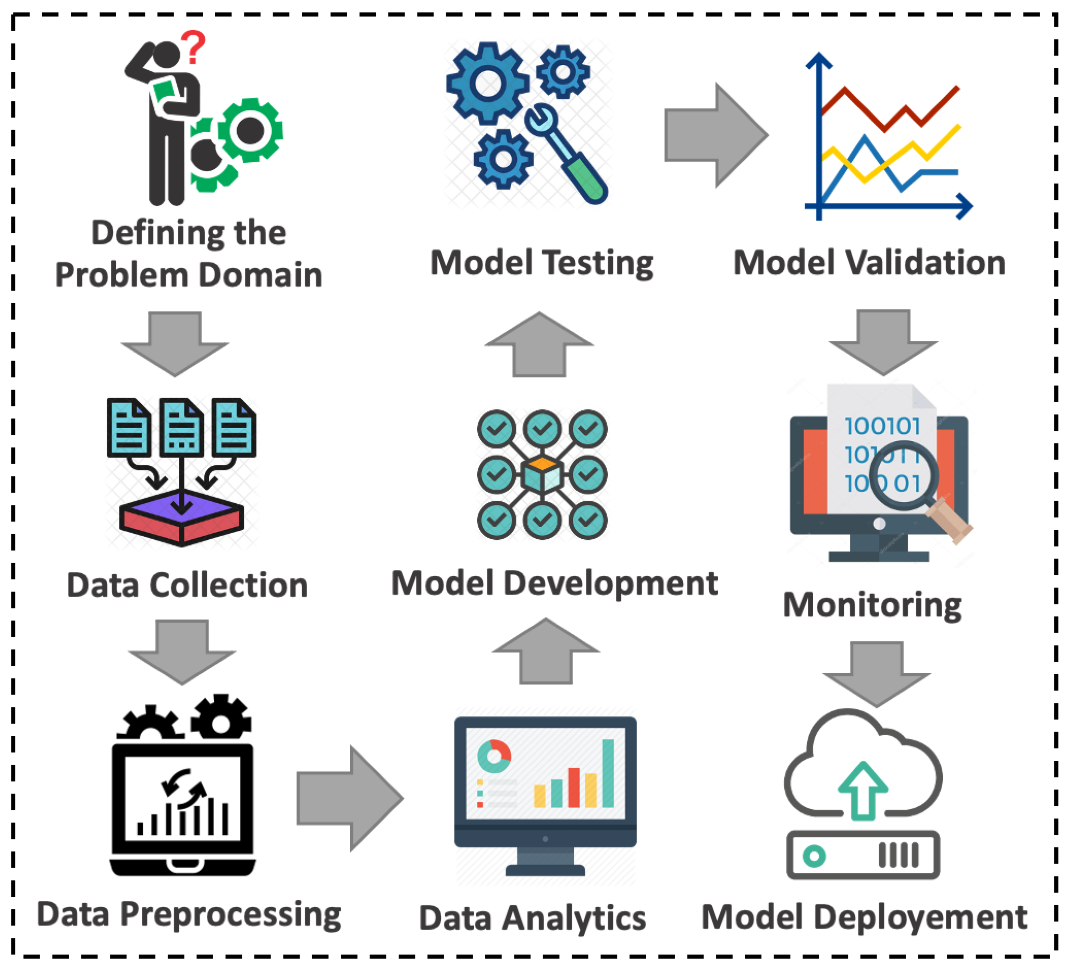
3. Materials and Methods

In this section, a series of steps are formulated, from handling data, and through scaling and transformation, to discovering the statistical properties of the data and modeling the deep learning approach as explained in the following subsections.

3.1. Dateset Handling and Per-Processing

Hourly PN concentration data for the area of Amman, Jordan, were collected from August, 2016 to July, 2017 at the Aerosol Laboratory, which is located at the third floor of the Department of Physics at the University of Jordan. The data contains PN concentration value with five meteorological parameters which are Temperature (T), Relative Humidity (RH), Pressure (P), Wind Speed (WS) and Wind Direction (WD). The data set contains 8784 records of six columns (five inputs and one output). The details of the aerosol measurements campaign and the meteorological measurements lie beyond the scope of this paper, and a detailed description can be found in previous studies [37,38].

A previous sensitivity analysis has been done on the dataset used in this work [28]. Each parameter has been investigated and tested in order to find the best combination of features to be used in the model. The results show that using a combination of the all parameters resulted in the best prediction accuracy. Having more than two parameters in the forecasting model which are interacting in a multi variant manner make the linear methods such as ARIMA may not be efficient in the prediction. A robust approach such as LSTM that can mimic non-linearity of the functions can be used to approximate regression and model PN concentrations.

All of the data are numeric, where the range of each column is different than the other. Before fitting a model and making the prediction, two data transforms operations are performed: (1) Checking, (2) Scaling and Transformation as explained below.

Checking: the database contained some lost data due to specialized and instrumental issues. These missing values were imputed by linear interpolation. Each data-base becomes reliable with the expected number of records.

Scaling and Transformation: The data transformation is important for the neural network training. One good data transform suggest the transformation of data to be within the same range as output of the activation function that is used in the model training. The Rectified linear unit (ReLU) is the most widely used activation function in the training of the neural network. It is provided by default from PyCharm environment, and its derivative values are between 0 and 1. A good scaling for the data is to transform it to fall within the same range. The MinMaxScaler function (defined in Equation (1)) provided by sklearn preprocessing library is used for this.

$$x_{-}scaled=x_{-}value\hspace{0.17em}\ast \hspace{0.17em}\left(max-min\right)\hspace{0.17em}+\hspace{0.17em}min$$

(1)

where $x_{-}scaled$ is the new scaled value, $x_{-}value$ is the original value, $max$ is the maximum value in the dataset observation and $min$ is the minimum value in the dataset.

The data are then transformed into a supervised data (input and output patterns). The previous observations of the previous time step are used as an input to the network at the current time step.

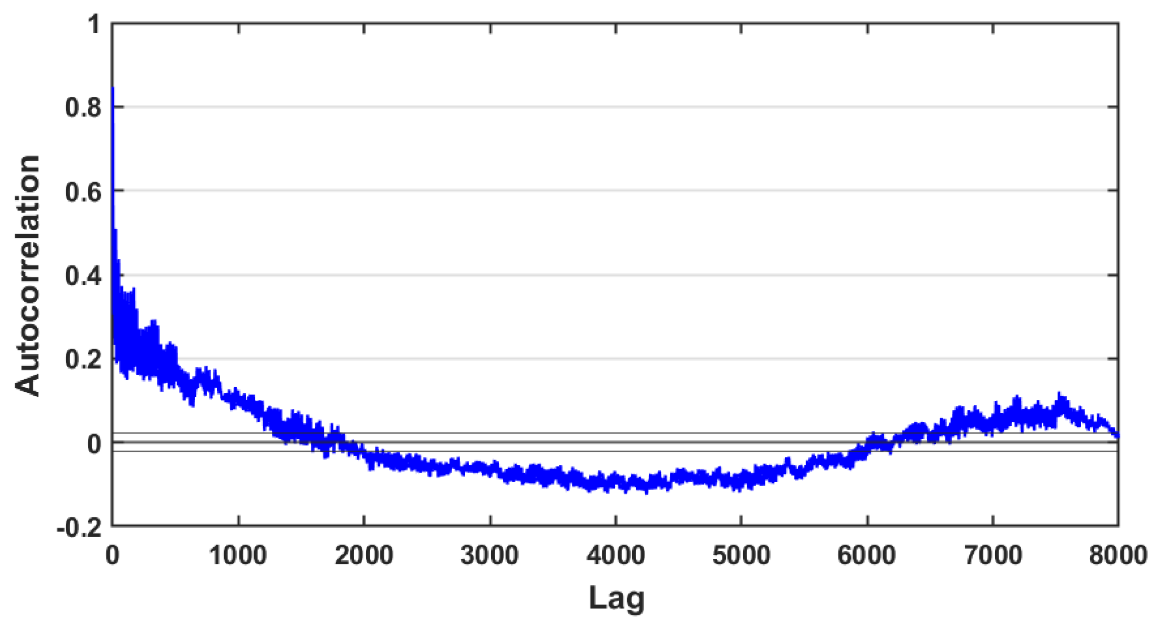
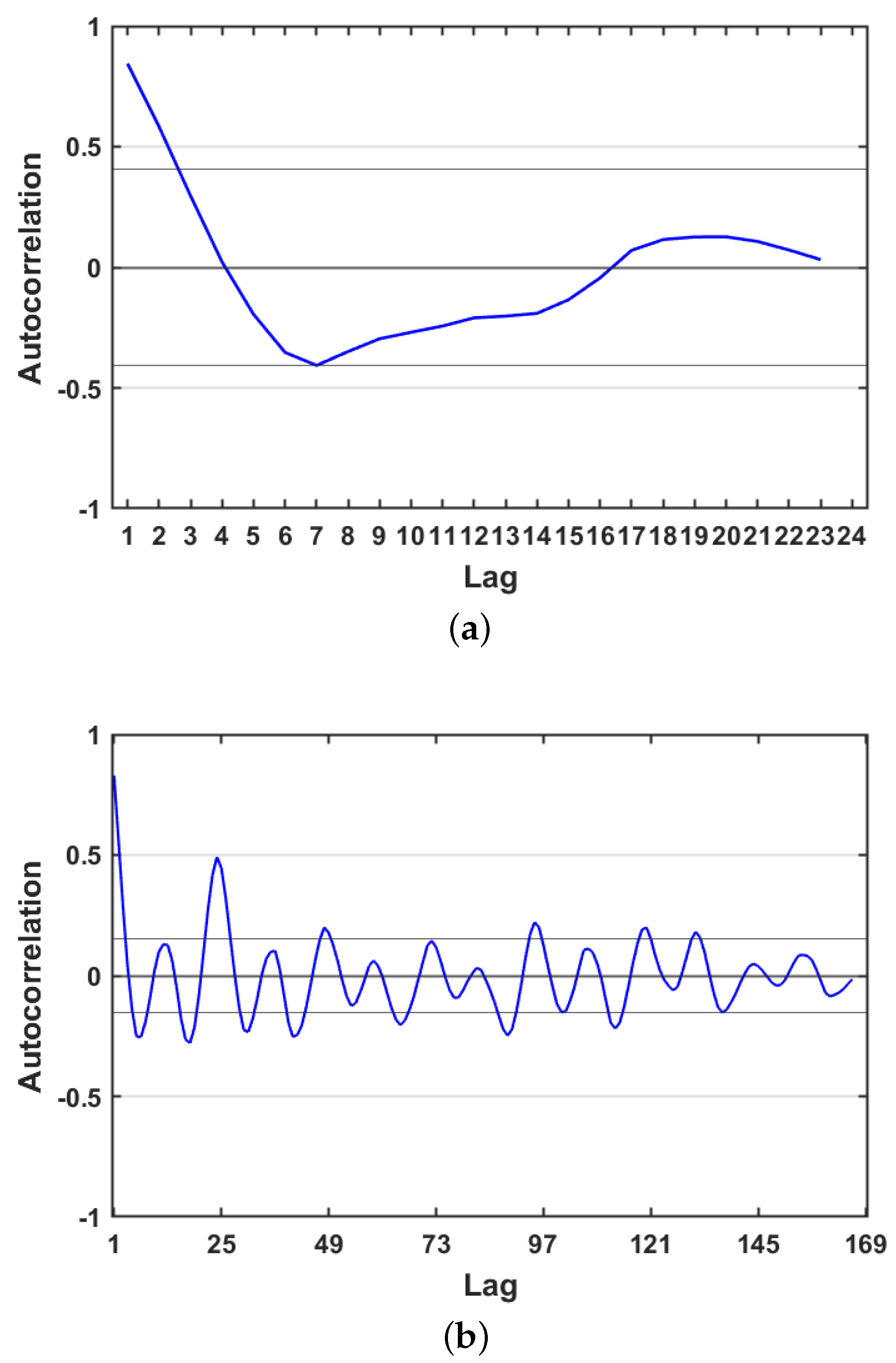
3.2. Data Statistical Analysis

The statistical method used in this paper is called Filter. It includes the application of two mathematical functions (Pearson’s correlation and autocorrelation) in order to extract a useful information about relationship between dependent and independent variables, and to find points where the behavior of PN concentration (dependent variable) changes. This point can be used later as a time-lag value.

The Pearson’s correlation coefficient r, as defined in Equation (2), was used to measure correlation between two parameters, the results are shown in

Table 2. Pearson’s coefficient between parameters.

	PN	T	RH	P	WS	WD
PN	1	−0.2475	0.0078	0.3389	−0.3113	−0.3320
T	−0.2475	1	−0.6909	−0.4463	0.3105	0.2836
RH	0.0078	−0.6909	1	0.1385	−0.0094	0.0718
P	0.3389	−0.4463	0.1385	1	−0.3481	−0.3323
WS	−0.3113	0.3105	−0.0094	−0.3481	1	0.6794
WD	−0.3320	0.2836	0.0718	−0.3323	0.6794	1

.

$$r=\frac{\sum (x_i-\overline{x})(y_i-\overline{y})}{\sqrt{\sum {(x_i-\overline{x})}^2\sum {(y_i-\overline{y})}^2}}$$

(2)

where $x_i$ is the value of x variable in the observations, $\overline{x}$ is the mean of all values of x. $y_i$ is the value of y variable in the observations and $\overline{y}$ is its mean.

The Pearson’s correlation coefficient is used here to analyse the relationship between two parameters only in order to investigate the importance of each input parameter in the prediction of PN concentrations. The number of input parameters to be used in the model construction is important to increase the accuracy and model performance. Notably, analyzing correlation between PN concentration and each of the meteorological parameters suggest the use of a combination of five meteorological data as input to model PN concentration. This result is compatible with the result obtained from the performing of previous sensitive analysis on the dataset [28].

Having more features in the training process will complicate the training process and may not necessarily improve the accuracy. If the included features are highly correlated with dependent variable (output), the accuracy will increase. On the other hand, if the included features are less correlated with dependent variable, this will increase complexity of the training by increasing the need for using more epochs, or increasing number of layers, number of neurons, etc., in order to generate a satisfactory result.

Then, autocorrelation function was used to measure hourly correlation of PN concentration. The autocorrelation function $Pk$ for a time delay k, can be defined as follows:

$$P=\frac{Cov\left(y\left(t\right),y\left(t+k\right)\right)}{\sigma y\left(t\right)\sigma y\left(t+k\right)}$$

(3)

where k is the time delay, $y\left(t\right)$ and $y(t+k)$ are the air pollutant concentrations at time t and $t+k$. The $Cov$ is the covariance and $\sigma$ is the standard deviation.

Applying the autocorrelation function on the hourly dataset shows the properties of the PN concentrations over the time horizon. As the data is a sequence of observations over time, it would be useful to know how much the observations at time $t-1$ affect the ones at time t. In Figure 2, a scatter plot shows the degree of the autocorrelation value shown on vertical axis in the data from t₀ to t₈₇₈₄.

On the graph, the value of the autocorrelation function for each lag is plotted. In order to capture the correlation of observations on the current status, the autocorrelation coefficient function is plotted for 24 h and 168 h (one week) as shown in Figure 3.

From Figure 3a an obvious descending trend can be observed in the PN concentration during the first period of time. Then it increases after 7 to 8 h to decrease again for the last 8 h of the day. Therefore, the PN concentrations are highly correlated with each other for the lag value equal to 8. The point where the concentration changes from decreasing to increasing trend or vice versa can be used to determine the time-lag value as a feature to perform forecasting.

A continuous and repeated pattern can be seen from Figure 3b for every 24 h. This means that the observations are highly correlated for this period of time and the value 24 can be used as a time-lag value.

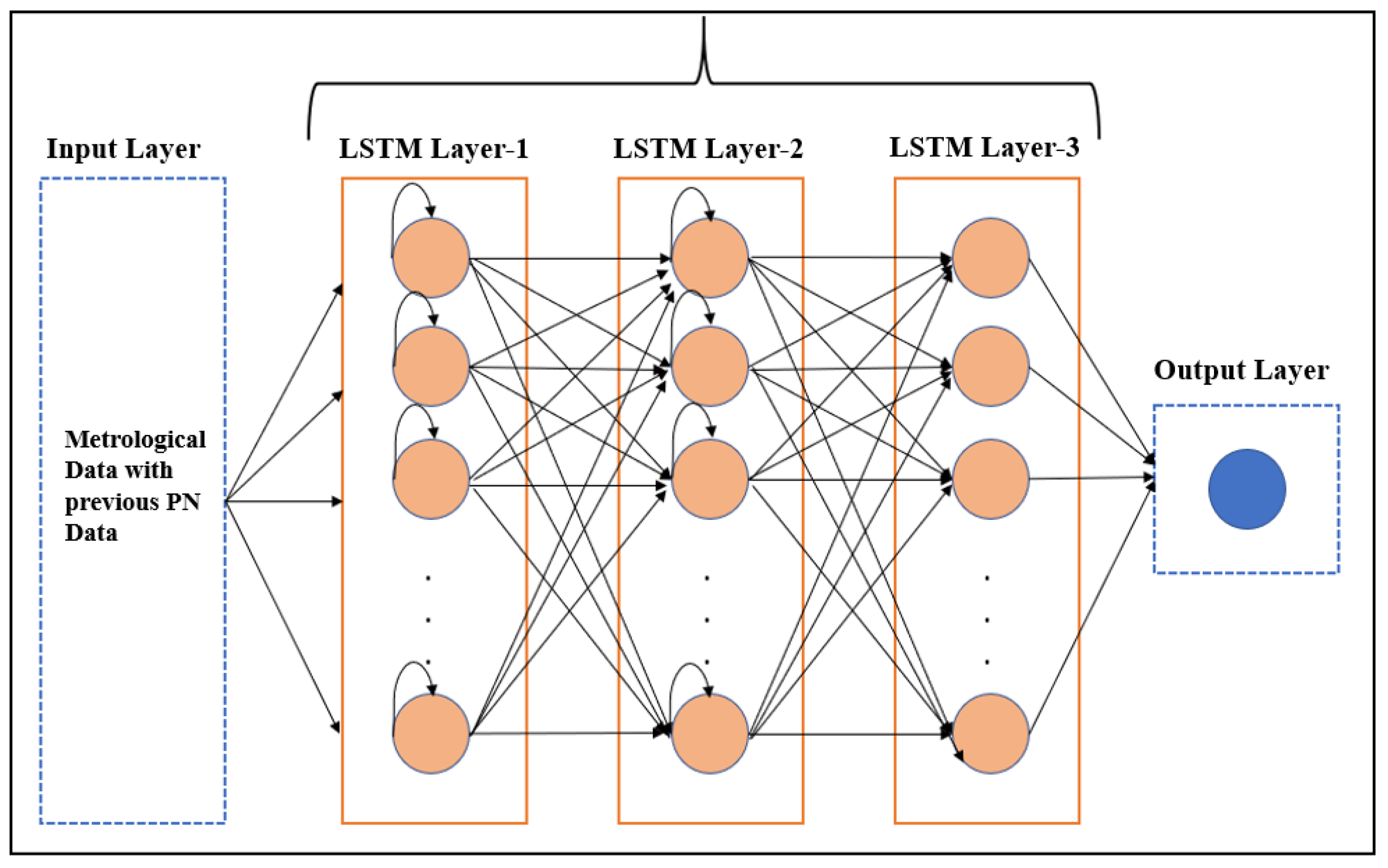
3.3. LSTM Model Setup

An alternative method to find time-lag value is to use an optimization algorithm such as GA. The GA can be applied on the features space of the predictive model to search for the optimal solution. Such method has the ability to find a good subset of solutions without investigating all possible subset of solutions. In this paper, the GA is applied on a predictive model developed by LSTM to search for optimal value of time-lag length feature. The reason of using LSTM model is the ability to perform a multi-step estimation given a data time window which makes it suitable for time-series forecasting.

The LSTM model used in this paper for PN concentration forecasting consists of one input layer, one output layer and three hidden layers. The configuration details of the LSTM hyperparameters are illustrated below and the overall architecture is shown in Figure 4.

Dataset Splitting: The dataset is split into two parts before the training: training set and testing set. The training set is used to build the model and fit it on the available data with known inputs and outputs. The testing set is used to estimate the model performance on unseen data (data not used to train the model). 80% of the dataset is allocated for the training and 20% of the dataset is allocated for testing.

Model Tuning: Several hyperparameters should be determined before starting prediction, such as learning rate, and number of epochs. The network parameters are changed through several experiments until reaching the stability of the network. The network becomes stable when the training error stops reducing after a specific value. At this point, the weights are optimized, and the changing of its value is very small which produce a very small, error change and can be negligible. In order to test the effect of each parameter and reach the network stability, several experiments were run using 10-fold cross validation over the training dataset where the value of one parameter is changed within a specific range and the others are kept fixed. The fold that generates the best accuracy will use its configuration as optimal choice for the investigated parameter. The k-fold cross validation method is a re-sampling technique that is usually used to estimate the model accuracy and avoid overfitting. The model is trained and tested in different subset of data in order to evaluate the model performance on the unseen data.

The number of hidden layers in the architecture and the number of neurons in each layer are determined by running the model several times, starting with one hidden layer. The hidden layers in the LSTM are recurrently connected and known as memory blocks. Each block consists of three main gates: Input, Forget and Output. The computation for each gate is done at each time step in the network and the equations of this calculations are given below:

$$i_t=\sigma \left(w_i\left[h_{t-1},x_t\right]+b_i\right)$$

(4)

$$f_t=\sigma \left(w_f\left[h_{t-1},x_t\right]+b_f\right)$$

(5)

$$f_t=\sigma \left(w_o\left[h_{t-1},x_t\right]+b_o\right)$$

(6)

where $i_t$ is the input gate, $f_t$ is the forget gate, $o_t$ is the output gate, $\sigma$ is the sigmoid function, $w_x$ is the weight of the gate x neurons, $h_t-1$ is the output of the previous time step, $x_t$ is the input of the current time step and $b_x$ is the bias of the current gate x. Equation (4) tells about the new input information to be stored at time t. Equation (5) describes the information to be thrown away and Equation (6) gives the activation of the final output of LSTM at current time t. The three gates provide continuous read, write and reset operations to make LSTM adequate to solve problems with long sequence and longer time steps.

To determine the number of hidden layers, the first experiment was done using one hidden layer, the accuracy was then evaluated. More hidden layers were added, and the accuracy was evaluated each time. After three hidden layers, there was no significant improvement in the forecasting accuracy.

The output layer is a regression layer with one neuron. The other network parameters are finalized based on the accuracy conducted. The training of the network is stopped after reaching the maximum number of epochs. A summary of LSTM configuration is given in

Table 3. LSTM configurations.

Network Parameter	Configuration
Number of hidden layers	3
Number of neurons at each hidden layer	50, 50, 10
Number of epochs	500
Optimizer	Adam
Batch size	32
Learning rate	0.001
Activation function	ReLU
Weight initialization	Normal distribution
Loss function	Mean square error

.

Model Testing and Validation: Four indicators are used to evaluate the effectiveness of each parameter, MAE, RMSE, MAPE and R-squared. MAE is used to measure the forecasting accuracy. It gives an indication about how the predicted values are far from the measured values. RMSE gives the square root of Mean Absolute Error (MSE) where MSE finds an average squared deviation of predicted values. It gives an overall idea about a generated error. MAPE measures the sum of the individual absolute errors divided by each individual separately. R-squared describes the strength of the relationship between the predicted values and the actual values. These indicators can be formulated as follows:

$$MAE=\frac{{\sum }_{i=1}^n\left|{\widehat{y}}_i-y_i\right|}{n}$$

(7)

$$RMSE=\left[\frac{1}{n}\sum _{i=1}^n{\left({\widehat{y}}_i-y_i\right)}^2\right]$$

(8)

$$MAPE=\frac{1}{n}\sum _{i=1}^n\frac{|y_i-\widehat{y_i}|}{y_i}$$

(9)

$$R-squared=1-\frac{{(y_i-{\widehat{y}}_i)}^2}{{(y_i-{\overline{y}}_i)}^2}$$

(10)

where n is the number of observations, y is the vector of the actual values and $\widehat{y}$ is the vector of the predicted values.

3.4. LSTM with Heuristic Algorithm

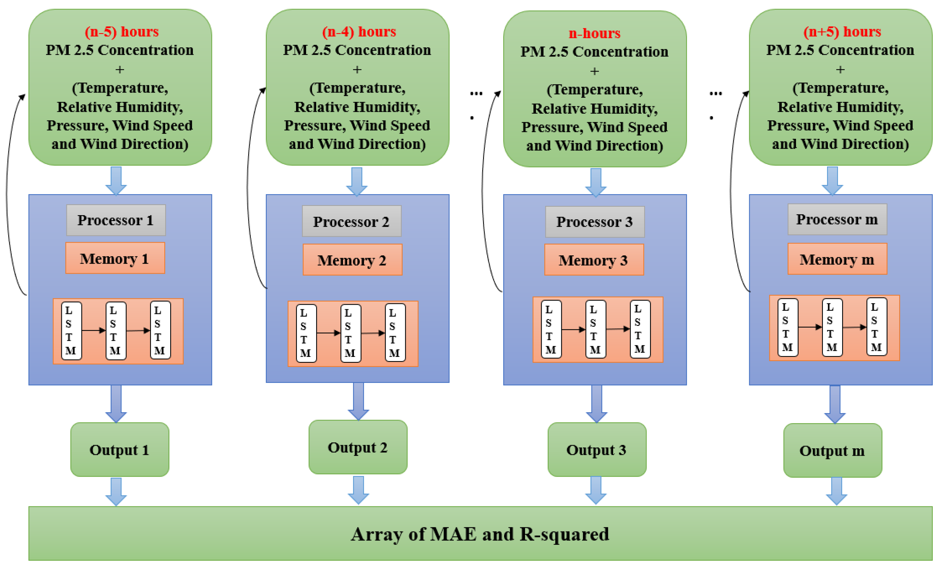
As mentioned before, the selection of the time-lag value can be done using several methods. In this paper, an optimization algorithm, genetic algorithm (GA), is used to find the best value of time-lag in LSTM model. GA [39] is a meta-heuristic algorithm that searches for the optimal solution by mimicking the process of evaluation by maximizing or minimizing some objective functions. It is used in the literature by numerous analysts within the computer science field to illustrate complex issues in an assortment of domains where the arguments of these issues may not be found in a sensible time [40]. Since it is simple to execute and can generate more accurate results, GA becomes one of the foremost prevalent used algorithms [39]. Because of its ability to generate a solutions which are close to the optimal solutions, GA has been applied in the literature to optimize the tuning of neural network architecture setups [41,42]. Comparing the rendering of GA with other optimization algorithms on understanding diverse sorts of complex optimization issue problems, several studies showed that GA performs better in the ideal arrangement and speedier than other strategies and methods including but not limited to Particle Swarm Optimizations (PSO), Differential Evolution (DE), and Ant Colony Optimization (ACO) [43,44,45,46,47].

The key components of GA are: population, operations (selection, crossover and mutation) and fitness function computation. The population y is initialized randomly. Then the fitness of each individual is calculated. Two individuals from the population are selected based on their fitness value. The crossover and mutation operations are then applied to produce new offsprings which are placed in the population. The operations are repeated on the current population until a new population is generated and the steps are rehashed for several cycles that guarantee the generation of good and satisfied results.

In our proposed model, GA is used on the training set to search for the optimal time-lag value for the forecasting model LSTM. The correct time-lag value can capture the dependencies among the successive observations. Using LSTM deep networks with a large number of parameters, finding the best lag value would computationally be expensive and time consuming. Therefore, GA is used in this paper not to guarantee the finding of the optimal time lag value, but to tend to produce the near global optimal solution that could be used by LSTM to enhance forecasting accuracy with the use of a proper time lag window. The size of GA population was set to 50. Each chromosome in the population represents a solution which is the possible number of the lag value. The first population was produced arbitrarily. Next, the fitness function is evaluated for each solution. The database was ready agreeing to the selected time-lag value and the model was then trained. LSTM generated the results and the MAE was then calculated for each solution and returned as a fitness value. Then, the main operations of GA are performed (selection, crossover and mutation), and the method was rehashed for several cycles. Finally, the solution with the most excellent fitness esteem score was chosen as the best solution.

3.5. Parallel Model

The computational time of the forecasting method is an important aspect to be considered. Although machine learning methods typically result in adequate results in forecasting accuracy, computational time remains one of major challenges to be solved. Therefore, an optimization process, which is proposed in this paper, aims to reduce the time required for finding the optimal time lag value sequentially.

A parallel algorithm implementation using a multi-core system can be used to search for the best time lag value in the forecasting process. In this case, two options can be resorted:

(1) running the model starting from the first time lag value (which is one) to the maximum value where each run can be done on one core of the system.

(2) investigate the model efficiency within a certain period of time lag value.

In the first case, more time is needed and it will exhaust resources in the case of limited resource availability. The second method is more efficient and will reduce time needed to find the best time lag value.

In this paper, the second method is used. In order to determine the required value of time lag that needs to be investigated on the multi-core system, the statistical analysis generated from the autocorrelation function is used. The statistical analysis provides a good suggestion for the best value to be used in the forecasting process. This proposed method can be applied if the time complexity must be reduced considerably while using a sequential forecasting method with no additional optimization technique such as GA.

The parallel implementation consists of 10 processors that run in parallel, where LSTM model is run on each processor with different time-lag values. As mentioned before, the autocorrelation coefficient function suggests a set of points where concentration has changed. For each point, a range of values around the point of interest were conducted and used to run LSTM model over 10 processors. For example, if the time-lag value is 7, then a range from 2 to 11 is conducted. Each value of time-lag within the range is fed to the LSTM processor, such that the 10 processors run in parallel with different time-lag values, and the result is then concluded.

The same indicators used to test accuracy of sequential LSTM are used here to test performance of each processor.

The indicators value of each processor output is saved in a list to compare them with each other. The processor that generates the least value of MAE and maximum of R-squared is conducted as the best predictor with the best value of time-lag. The overall architecture of parallel LSTM for n time-lags is shown in Figure 5.

4. Empirical Results and Discussion

In this section, we present the result of time-lag value selection generated by each method:

(i)

The statistical method that are based on autocorrelation coefficient function. This method will suggest the value of time-lag based on correlation that is shown by the autocorrelation function

(ii)

The LSTM with GA. GA will search for the best time-lag value to be used for the prediction. The solution with lowest MAE (fitness function) will be considered to be an optimal solution.

(iii)

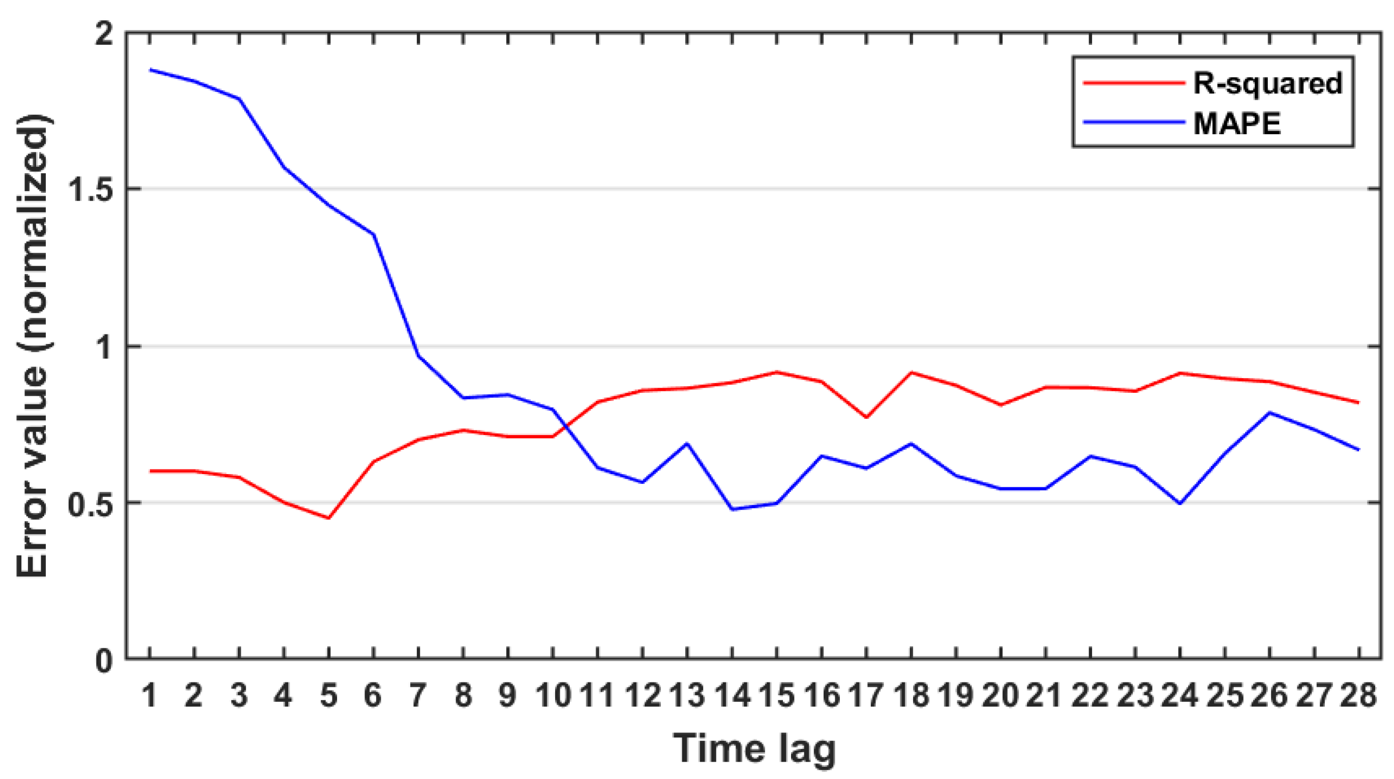
The parallel LSTM. The LSTM model will run in parallel over different processors with different time lag. The MAE, RMSE, MAPE and R-squared are taken for the performance evaluations among them. The processor with lowest MAE, RMSE, MAPE and highest R-squared will be considered to be the best prediction result where the time-lag used by it will be the best lag value.

4.1. Statistical Results

The statistical analysis of Pearson correlation function can be useful for the feature selection before training the predictive model. Training the model with a set of inputs (independent variables) that show a good correlation with output (dependent variables) will increase accuracy and enhance performance. While having more input parameters with less correlation increases complexity of training by increasing running time, this does not generate better results.

The analysis of autocorrelation function includes analysis of Figure 3a,b to capture the time point when behavior of concentration changes within 24 h and 7 days. Figure 3a shows an obvious descending trend in the correlation with increasing time-lags. It continues decreasing until reaching the time-lag 7. This means that previous events are highly correlated. After that, the curve goes up, which indicates that the correlation increases until it reaches the time-lag 15 and so on.

Figure 3b shows the behavior of autocorrelation function of PN for one week (168 h). The pattern of the function is repeated every 24 h until the end of the week. The PN concentration decreases in the last two days of the week (from hour 120 to hour 168), which indicares that the correlation between the observations on the working days (five days of the week) is different from the correlation between the observations at the weekend. PN concentration decreases during the weekend because the pollution emission, such as such as vehicular combustion, is less during weekend. To reduce the problem complexity, the 24-h period can be chosen for the time-lag value.

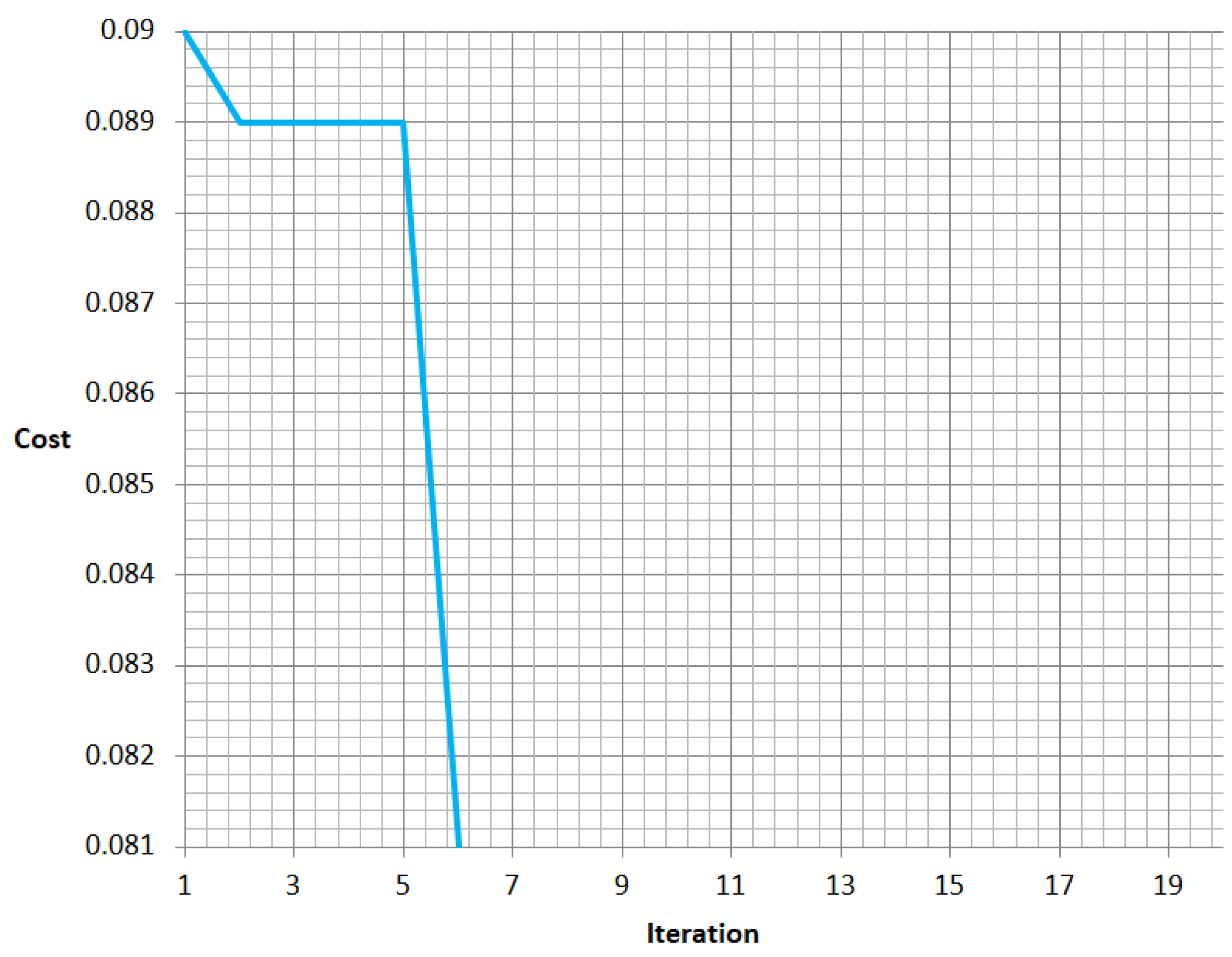
4.2. LSTM and GA Results

The points of interest of applying GA on LSTM to find the ideal time-lag esteem are:

• Initial population: The range of time-lag to be tested is from 1 to 24. A binary vector randomly initializes using uniform distribution defined initial solution. The population is set to have 50 possible solutions.
• Selection: Select the best fitness values of two individuals from the population (parents).
• Crossover: Trade the variables between chosen parents to generate new off springs. One-point crossover is used for that.
• Mutation: A binary bit flip with probability of 0.1 is connected with the solution pool by arbitrarily swapping bits to realize differing qualities on the solutions.
• Fitness function: MAE is used to evaluate solution.

The dataset is split into training and testing, where the size of the training dataset is minimized to speed up the search handle of GA. The generated solution from GA is used to train LSTM model and is validated on the testing set. The solution that gives best fitness score is chosen as the best solution. Figure 6 summarizes the results of MAE (fitness function) of different time-lag selected by GA and

Table 4. MAE, RMSE, MAPE and R-squared values with time-lag of 21 for LSTM with GA method.

MAE	RMSE	MAPE	R-Sqaured
0.020	0.022	0.053	0.90

gives the four evaluation metrics value that are generated from LSTM model with time lag value of 21.

It can be concluded from Figure 6 that LSTM model performed poorly with a small time-lag value selected by GA. GA searched for the best solution. The accuracy enhanced when the time-lag increases. The results for time-lag interval (21:23) are the best with minimum MAE value.

The using of GA to solve non-deterministic polynomial time (NP) problem that requires the searching for optimal solution is effective. The pitfall of using such method is running time. Because GA performs four operations on its population, the searching procedure for the optimal solution consumes time. As more data are added, the population increases and therefore more time is needed to generate the required solution [23].

The convergence speed for the GA was computed using the dataset as presented in Figure 7, which shows how the fitness gradually decreases across the iterations and confirms that the GA escapes the local minima in the time series dataset and is able of find the best hyperparameter values for the LSTM in less than 9 iterations.

These results agree with [48], which showed that random search of the hyperparameters for the deep neural networks might take a long time to converge and achieve good results as training the deep neural networks using large parameters number for each selected hyperparameter is actually very time-consuming.

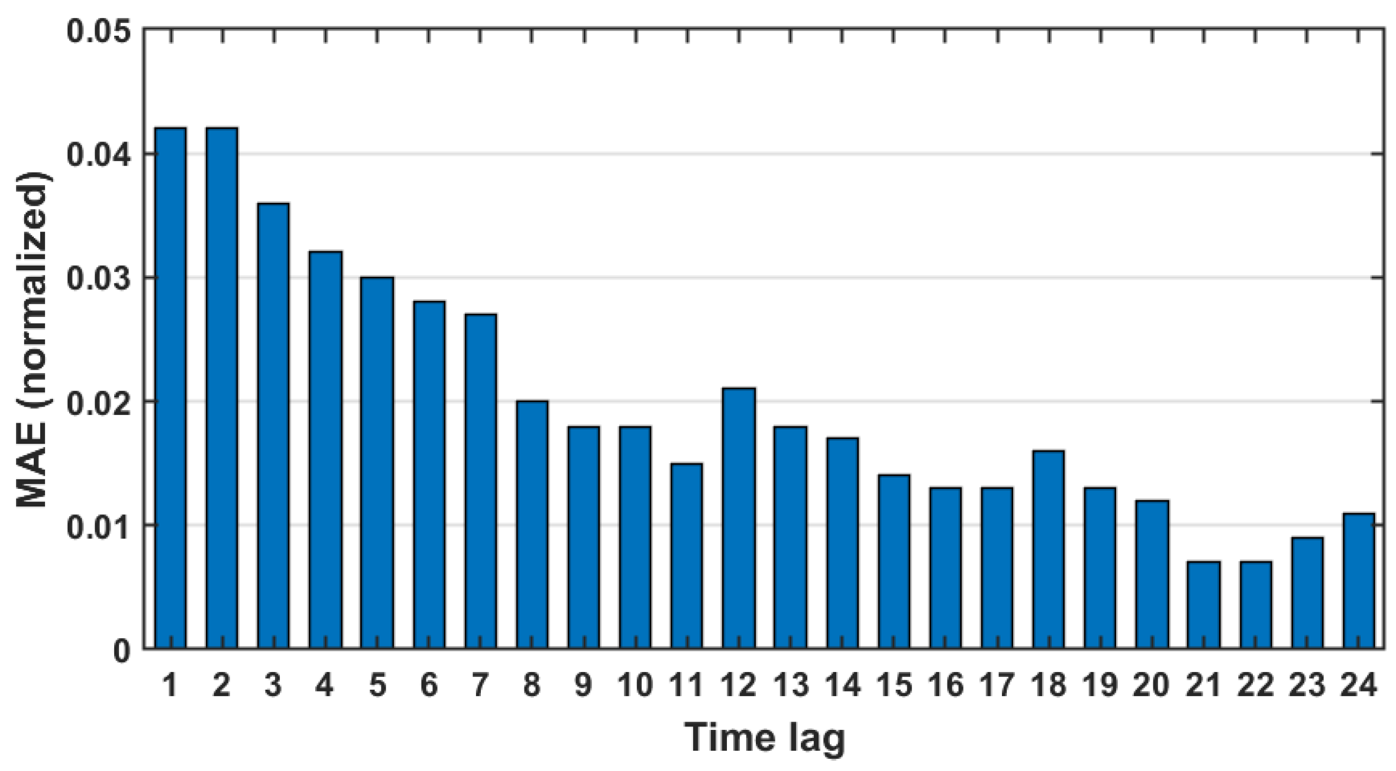
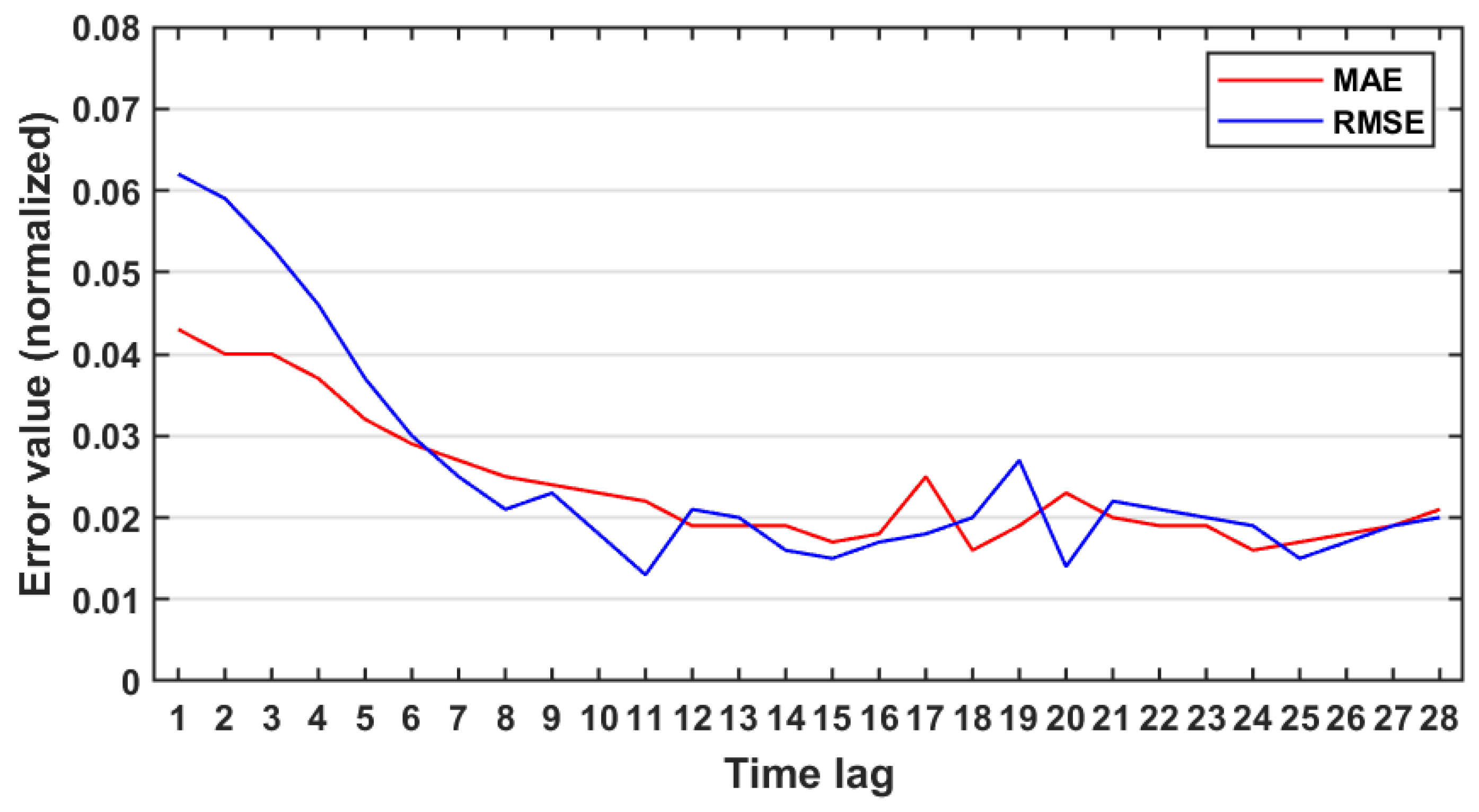
4.3. Parallel LSTM Results

In the parallel experiments, two time-lag values were tested, 6 and 24. The previous statistical analysis shows a high correlation between the observations close to these values.

For the time-lag 6, ten processors were run in parallel, where each processor took the same LSTM configuration but with a different time-lag value. The first processor took the time-lag value 1, the next took the time-lag 2 and the last tested the performance of LSTM with the time-lag value 11. For the performance evaluation, MAE, RMSE, MAPE and R-squared were calculated from each processor output.

The output of parallel implementation for the time-lag values were generated and saved in an array. A comparison between these values shows that the best output can be obtained when the time-lag is equal to 10 with the smallest MAE, RMSE and the highest R-squared value. The results show that increasing number in the time-lag value increases accuracy with the decreasing in MAE, RMSE and MAPE values. There is a decreasing trend in the R-squared value with small time-lag values (from 1 to 5). This indicates that although there is an enhancement in terms of accuracy as MAE and RMSE values show, there is no linear relationship between actual and predicted values as indicated by the low R-squared for small time-lags. The goodness of fit for the observations is not good for small lag values where data points that fall in the regression line are not much as those for larger lag values. This result demonstrates that small time-lag values are not suitable to be chosen.

To investigate the influence on the increasing time-lag value, the experiment repeated twice with different ranges, one in the range (11:20) and the other in the range (21:28) in order to investigate the values of time-lag window for one day. The results are shown in Figure 8 and Figure 9.

The dynamic selection of time-lag value using parallel implementation can help in improving the performance of the LSTM in terms of accuracy. The time-lag parameter has a good influence on increasing or decreasing prediction accuracy. If the data within the range of the selected time-lag values is correlated, then the prediction is improved and the accuracy will be high. If the time-lag is selected randomly, where the data within that time is not correlated, the performance of the LSTM will be decreased by generating a less accurate result.

The effect of the changing in time-lag values on the model performance is shown in Figure 8 and Figure 9. A decrease in the error values (MAE, RMSE and MAPE) is generated by increasing time-lag values. After the time-lag 6, the calculated errors change slowly and levels off at time-lag value 20. Comparing the R-squared values, the correlation between predicted and actual observations is increasing by time. From the time-lag value 20 onward, a decrease in the error is noticeable for the lag interval (21:24) with an increase in the R-squared. The time-lag value 24 could be the best due to the high correlation between the actual and the predicted value.

4.4. Discussion

Three methods have been used in this paper to investigate the effect of choosing optimal time-lag value in the performance of prediction model. Each method has its advantages and disadvantages. Statistical method using Pearson correlation function and autocorrelation function shows that the earlier events have a weak influence on the PN concentrations, which means that the value of time-lag between 1 and 8 is not strong to be selected when training the model. The autocorrelation function shows that by increasing the time-lags, the correlation increases with concentrations. A repeated pattern could be noticed for daily hours with a small change at the end of the day.

The statistical method is precise and gives a good indication about the behavior of data correlation. It can be used to suggest appropriate time-lag value that will be used later as a parameter of deep learning prediction model. Indeed, the statistical results are close to the sequential results conducted when using GA to select the appropriate time-lag value. GA gives the best time-lag value to be used to predict the PN concentration, which falls in the interval (21:23). This result means that the using of heuristic algorithm prove that better performance can be generated that is close to the statistically accurate result generated by autocorrelation function.

Heuristic algorithm is an optimization method that can be applied to search for the best solution. In the problem investigated in this paper, GA was used and found the optimal solution for the time-lag selection problem.

Although the solution generated by the GA is compatible with the mathematical solution (generated by autocorrelation function). This means that GA can find the optimal solution for this problem. It is known that heuristic algorithms may lead to the optimal solution or near the optimal solution when solving a large problem. In our work, GA outperforms the traditional methods and finds the optimal solution which makes our model more robust and its results more reliable. On the other hand, LSTM networks suffer from some weakness in terms of accuracy and learning speed due to the long-term dependencies in the forecasting problem [49]. These issues need to be solved and optimized by the proper tuning of LSTM parameters. In this paper, we investigated the effect of selecting the proper time lag value on the forecasting accuracy which can be done by applying traditional methods such as autocorrelation function or the state-of-the-art method such as the heuristic algorithm. The decision of using this method depends on the priority of performance evaluation metrics such as accuracy, speed, etc.

The parallel implementation method suggests the time-lag value 24 is the best. The parallel implementation searches for the best value dynamically by running a loop with a specific range. Using this method is preferable when the time issue is important. The results are optimized in terms of time and accuracy, as the last value will be selected based on MAE and R-squared value. This method is accurate and efficient and can be used depending on the problem requirements and the resources available.

A comparison between the LSTM with GA model and the parallel LSTM model in terms of processing time and accuracy is presented in

Table 5. MAE variations over different time-lag value for LSTM with GA method and parallel LSTM method.

Time lag value	22	23	24
LSTM with GA (MAE)	0.009	0.012	0.013
Parallel LSTM (MAE)	0.019	0.019	0.016
LSTM with GA/Processing time	19.423	23.604	29.183
Parallel LSTM/Processing time	24.745	25.254	29.678

with different time-lag values used by each method.

The experimental results show that heuristic algorithm could help find the optimal time-lag value and be applied to LSTM, and it gives the best prediction with lowest error rate. For a specific and pre-defined range of time-lag value, the parallel processors can generate the best prediction accuracy. As shown in

Table 6. Performance comparison between the proposed LSTM model with GA and ANN, LSTM, GRU, and BRNN.

Model	MAE	Running Time
LSTM with GA	0.012	7.353
ANN [28]	0.035	3.452
LSTM [23]	0.028	9.128
GRU [23]	0.041	7.534
BRNN [23]	0.037	17.798

, the processor with time-lag value generates the lowest MAE. This value is greater than error generated by optimal lag value which is selected by GA.

Another comparison is made between the current approaches used in this paper and previous methods that have been proposed and run on the same dataset [23,28]. In [28], the authors proposed a framework using ANN, and in [23] the authors used LSTM, Gated Recurrent Networks (GRU) and Bi-directional Recurrent Neural Network (BRNN) to model PN concentrations. The results of these works with a selected time-lag value equal to 1 are compared with the results conducted by the proposed approach in this paper that used LSTM with a selected time-lag by GA along with the time needed to run each method in order to investigate the difference between them in terms of time complexity. The comparison is listed in Table 6.

The information provided in Table 6 shows how the traditional machine learning method, ANN, has the lowest running time while the superiority goes to the BRNN method. As BRNN runs in both directions, it is expected to have the highest time complexity.

A small increase in the running time appears when we apply GA on the LSTM method. While the MAE for LSTM with GA is the smallest. The optimization in the machine learning method can be achieved by considering one or more evaluation metrics. The enhancement in the accuracy obtained from the application of GA with LSTM increases on the other hand the time complexity.

Figure 10 shows how each method approximates the modelling of PN concentrations. The vertical axis shows the MAE and the horizontal axis shows the accuracy of model fit. The results are reported for each method with time lag value = 1 (one-step-ahead forecasting). The accuracy of how the model fits the historical data can be defined as follows [3]:

$$ModelFitting\left(MF\right)=\frac{\left(n{\sum }_{t=1}^n{\left(y_t-\widehat{y_t}\right)}^2\right)}{{\left({\sum }_{t=1}^n{y}_t\right)}^2}$$

(11)

It is evident from the Figure that the model with lowest model fit error (LSTM) does not guarantee the most accurate result. The ordinary LSTM has some drawbacks such as computational complexity and overfitting. In this case, more efforts are needed to decide when to stop the optimization process and consider the pattern as the type of the noise of data [3]. Some of the state-of-the-art works aim to optimize the performance of the original LSTM using different optimization methods to benefit from its advantage in sequence processing and avoids its drawbacks. Therefore, in this paper an optimized model of LSTM with GA to proper select time lag value is presented to effecienty predict time-series.

The using of the proper time-lag value in the forecasting model reduces the error and increases the prediction accuracy. The LSTM model with the selected time-lag value with the smallest error value (23 in this study) found by GA outperforms other approaches. The use of heuristic algorithm optimizes the model performance and avoids the running of several experiments to optimal model accuracy. Therefore, it can be said that for time-series forecasting model, the time-lag parameter is very important and is able to affect the prediction accuracy.

In general, the selection of time-lag parameter value is important when using LSTM model for time-series forecasting problems. Using the appropriate value will influence the prediction accuracy. Some recommendations can be summarized as follows:

(i)

The statistical method depends on using mathematical function, autocorrelation function. It requires a prior knowledge about the data domain in order to select the proper parameter. It is good to capture the linear relationship between observations at time t and at previous time t − 1 and gives an obvious result about correlation between observations.

(ii)

GA is a heuristic algorithm that searches for optimal solution for a given problem by repeatedly applying specific operations on the population of the problem. The heuristic algorithm guarantees the generation of satisfactory solution, but it could not be the best. It is recommended to use it if the dataset of the given problem is not too big. The running time of GA is large, and it increases as the search space of the algorithm increases.

(iii)

The parallel implementation that searches for optimal time-lag dynamically is recommended if the parallel resources become available. It gives the best result from a given input range, and a high forecasting accuracy can be obtained from this method. For large dataset and big data problem, it is recommended to run such model on high-performance computers, such as super computers.

(iv)

Comparing methods in terms of processing time shows that LSTM with GA needs more time to generate accurate results. This is because GA is a search optimized algorithm, which searches for the optimal solution depends on the dataset size. For larger datasets, more time will be needed to guarantee the generation of optimal solution.

(v)

The experimental results show that heuristic algorithm could find the optimal time-lag value and it could be applied to LSTM, resulting the best prediction accuracy with lowest prediction error. This method can be applied to any time-series applications and complex data.

(vi)

Deciding which category (statistical or machine learning) of methods to be used for choosing time lag value depends on the dataset and linearity in the relationship between inputs and outputs. There are thousands of works in the literature that apply neural networks on the time-series forecasting. Few of these works investigate the effect of parameter selection on the forecasting accuracy and model performance. Recent studies such as [50] proposed the use of LSTM to analyze the changes in Air Quality Index and time-series data of Nanjing were used. The study in [51] combined Semi-Supervised Classification and Semi-Supervised Clustering machine learning methods for air pollutants prediction and showed how it can be used successfully for time-series prediction problem. The work in [52] compared statistical and deep learning methods in time-series forecasting. However, both statistical and deep learning methods (such as LSTM) are useful to be used in the time-series applications, a comparison between these methods can be investigated with respect to more than one consideration such as time-lag parameter selection. This is exactly what is investigated in this work.

(vii)

In the time-series applications, the default time-lag value used is usually one. Few studies aimed to find the optimal lag value to be used in the forecasting model where the model observations are highly correlated. Finding this value can be done using different methods as mentioned before. The aim of this research is to set up a vector between the determination strategies to contextualize which one is the best and for which setting.

(viii)

This study differs from other similar studies in the following aspects: (1) Dataset, the type of the data being used is PN concentrations in Amman, Jordan. (2) The setting of LSTM model which is used for the comparative analysis.

(ix)

The method used in this paper may be less efficient if the amount of dataset were massive. Additional experiments would be done by including more variables that may have impacts on the estimation of PN concentrations in Jordan and other different locations.

(x)

Despite differences between this study and other similar studies in the literature, the proposed results can be extended to be used into wider scientific areas especially in time-series forecasting applications.

5. Conclusions

This paper presents a comparison between three methods to find the optimal time-lag value for the time-series forecasting model. The three methods include the use of the statistical autocorrelation function, a hybrid optimized method of LSTM and genetic algorithm and a parallel dynamic selection based on LSTM method. The aim is to select a proper time-lag value that can be used in the forecasting process to generate an accurate result and reduce the non-linear dimensionality of the training process. An hourly dataset for PN concentration of Amman, Jordan is used to estimate accuracy of each method. The accurate estimation of PN concentrations is an essential part of air pollution prediction system.

The results show that the use of heuristic algorithm to search for the optimal time-lag parameter value has optimized the performance of prediction model by generating the lowest error rate.

The autocorrelation function gives a strong indication about correlation between time-series observations. The observations for a given time-lag are highly correlated and can be shown from plotting the relationship between the estimated value and time. The value of time-lag can be conducted from checking the plotted figures manually. This value is used in the parallel implementation as a range of values run at the same time on a multiprocessor environment to end up with the result of the lowest error rate between them.

Nevertheless, the performance of LSTM model which is used in this paper might be changed as the dataset size increased. More variables can be included that affects the estimation of PN concentrations. This might need to evaluate the same model with different sized datasets in order to capture the point where the model performance varies.

As future work, we plan to generalize the model by applying it with more datasets with different locations rather than solely in Jordan. The performance of the forecasting process can be further improved using more optimized methods such as combination of convolutional neural networks and other machine learning techniques. The effectiveness of network parameters can be investigated to urge the network to generate more accurate results from the proper configurations. In addition, we plan to include additional inputs such as the past data of PN along with meteorological variables that would increase the accuracy and robustness of the models’ predictions. Finally, the performance of the neural network model depends mainly on the problem domain and its dataset. More experiments can be investigated over different datasets with various volumes.

References

1. Fattah, J.; Ezzine, L.; Aman, Z.; El Moussami, H.; Lachhab, A. Forecasting of demand using ARIMA model. Int. J. Eng. Bus. Manag. 2018, 10, 1847979018808673. [Google Scholar] [CrossRef] [Green Version]
2. Tealab, A.; Hefny, H.; Badr, A. Forecasting of nonlinear time series using ANN. Future Comput. Inform. J. 2017, 2, 39–47. [Google Scholar] [CrossRef]
3. Makridakis, S.; Spiliotis, E.; Assimakopoulos, V. Statistical and Machine Learning forecasting methods: Concerns and ways forward. PLoS ONE 2018, 13, e0194889. [Google Scholar] [CrossRef] [PubMed] [Green Version]
4. LeCun, Y.; Bengio, Y.; Hinton, G. Deep learning. Nature 2015, 521, 436–444. [Google Scholar] [CrossRef]
5. Precup, R.E.; Teban, T.A.; Albu, A.; Borlea, A.B.; Zamfirache, I.A.; Petriu, E.M. Evolving fuzzy models for prosthetic hand myoelectric-based control. IEEE Trans. Instrum. Meas. 2020, 69, 4625–4636. [Google Scholar] [CrossRef]
6. Bengio, Y.; Boulanger-Lewandowski, N.; Pascanu, R. Advances in optimizing recurrent networks. In Proceedings of the 2013 IEEE International Conference on Acoustics, Speech and Signal Processing, Vancouver, BC, Canada, 26–31 May 2013; pp. 8624–8628. [Google Scholar]
7. Amberkar, A.; Awasarmol, P.; Deshmukh, G.; Dave, P. Speech recognition using recurrent neural networks. In Proceedings of the 2018 International Conference on Current Trends towards Converging Technologies (ICCTCT), Coimbatore, India, 1–3 March 2018; pp. 1–4. [Google Scholar]
8. Zaidan, M.A.; Motlagh, N.H.; Fung, P.L.; Lu, D.; Timonen, H.; Kuula, J.; Niemi, J.V.; Tarkoma, S.; Petäjä, T.; Kulmala, M.; et al. Intelligent calibration and virtual sensing for integrated low-cost air quality sensors. IEEE Sens. J. 2020, 20, 13638–13652. [Google Scholar] [CrossRef]
9. Motlagh, N.H.; Lagerspetz, E.; Nurmi, P.; Li, X.; Varjonen, S.; Mineraud, J.; Siekkinen, M.; Rebeiro-Hargrave, A.; Hussein, T.; Petaja, T.; et al. Toward massive scale air quality monitoring. IEEE Commun. Mag. 2020, 58, 54–59. [Google Scholar] [CrossRef]
10. Mahata, S.K.; Das, D.; Bandyopadhyay, S. Mtil2017: Machine translation using recurrent neural network on statistical machine translation. J. Intell. Syst. 2019, 28, 447–453. [Google Scholar] [CrossRef] [Green Version]
11. Nabavi, S.A.; Motlagh, N.H.; Zaidan, M.A.; Aslani, A.; Zakeri, B. Deep Learning in Energy Modeling: Application in Smart Buildings with Distributed Energy Generation. IEEE Access 2021, 9, 125439–125461. [Google Scholar] [CrossRef]
12. Nabavi, S.A.; Aslani, A.; Zaidan, M.A.; Zandi, M.; Mohammadi, S.; Hossein Motlagh, N. Machine learning modeling for energy consumption of residential and commercial sectors. Energies 2020, 13, 5171. [Google Scholar] [CrossRef]
13. Belavadi, S.V.; Rajagopal, S.; Ranjani, R.; Mohan, R. Air quality forecasting using LSTM RNN and wireless sensor networks. Procedia Comput. Sci. 2020, 170, 241–248. [Google Scholar] [CrossRef]
14. Moghar, A.; Hamiche, M. Stock market prediction using LSTM recurrent neural network. Procedia Comput. Sci. 2020, 170, 1168–1173. [Google Scholar] [CrossRef]
15. Jammalamadaka, S.R.; Qiu, J.; Ning, N. Predicting a stock portfolio with the multivariate Bayesian structural time series model: Do news or emotions matter? Int. J. Artif. Intell. 2019, 17, 81–104. [Google Scholar]
16. Nguyen, H.P.; Baraldi, P.; Zio, E. Ensemble empirical mode decomposition and long short-term memory neural network for multi-step predictions of time series signals in nuclear power plants. Appl. Energy 2021, 283, 116346. [Google Scholar] [CrossRef]
17. Ghoniem, R.M.; Shaalan, K. FCSR-fuzzy continuous speech recognition approach for identifying laryngeal pathologies using new weighted spectrum features. In Proceedings of the International Conference on Advanced Intelligent Systems and Informatics, Cairo, Egypt, 9–11 September 2017; Springer: Berlin/Heidelberg, Germany, 2017; pp. 384–395. [Google Scholar]
18. Peng, L.; Liu, S.; Liu, R.; Wang, L. Effective long short-term memory with differential evolution algorithm for electricity price prediction. Energy 2018, 162, 1301–1314. [Google Scholar] [CrossRef]
19. Feurer, M.; Hutter, F. Hyperparameter optimization. In Automated Machine Learning; Springer: Cham, Switzerland, 2019; pp. 3–33. [Google Scholar]
20. Velliangiri, S.; Karthikeyan, P.; Xavier, V.A.; Baswaraj, D. Hybrid electro search with genetic algorithm for task scheduling in cloud computing. Ain Shams Eng. J. 2021, 12, 631–639. [Google Scholar] [CrossRef]
21. Kan, X.; Fan, Y.; Fang, Z.; Cao, L.; Xiong, N.N.; Yang, D.; Li, X. A novel IoT network intrusion detection approach based on Adaptive Particle Swarm Optimization Convolutional Neural Network. Inf. Sci. 2021, 568, 147–162. [Google Scholar] [CrossRef]
22. Wu, T.; Feng, F.; Lin, Q.; Bai, H. Advanced Method to Capture the Time-Lag Effects between Annual NDVI and Precipitation Variation Using RNN in the Arid and Semi-Arid Grasslands. Water 2019, 11, 1789. [Google Scholar] [CrossRef] [Green Version]
23. Surakhi, O.M.; Zaidan, M.A.; Serhan, S.; Salah, I.; Hussein, T. An Optimal Stacked Ensemble Deep Learning Model for Predicting Time-Series Data Using a Genetic Algorithm—An Application for Aerosol Particle Number Concentrations. Computers 2020, 9, 89. [Google Scholar] [CrossRef]
24. Zaidan, M.A.; Mills, A.R.; Harrison, R.F.; Fleming, P.J. Gas turbine engine prognostics using Bayesian hierarchical models: A variational approach. Mech. Syst. Signal Process. 2016, 70, 120–140. [Google Scholar] [CrossRef]
25. Bouktif, S.; Fiaz, A.; Ouni, A.; Serhani, M.A. Optimal deep learning lstm model for electric load forecasting using feature selection and genetic algorithm: Comparison with machine learning approaches. Energies 2018, 11, 1636. [Google Scholar] [CrossRef] [Green Version]
26. Wang, Y.; Lin, K.; Qi, Y.; Lian, Q.; Feng, S.; Wu, Z.; Pan, G. Estimating brain connectivity with varying-length time lags using a recurrent neural network. IEEE Trans. Biomed. Eng. 2018, 65, 1953–1963. [Google Scholar] [CrossRef]
27. Lim, Y.B.; Aliyu, I.; Lim, C.G. Air Pollution Matter Prediction Using Recurrent Neural Networks with Sequential Data. In Proceedings of the 2019 3rd International Conference on Intelligent Systems, Metaheuristics & Swarm Intelligence, Male, Maldives, 23–24 March 2019; pp. 40–44. [Google Scholar]
28. Zaidan, M.A.; Surakhi, O.; Fung, P.L.; Hussein, T. Sensitivity Analysis for Predicting Sub-Micron Aerosol Concentrations Based on Meteorological Parameters. Sensors 2020, 20, 2876. [Google Scholar] [CrossRef]
29. Li, X.; Peng, L.; Yao, X.; Cui, S.; Hu, Y.; You, C.; Chi, T. Long short-term memory neural network for air pollutant concentration predictions: Method development and evaluation. Environ. Pollut. 2017, 231, 997–1004. [Google Scholar] [CrossRef]
30. Ribeiro, G.H.; Neto, P.S.d.M.; Cavalcanti, G.D.; Tsang, R. Lag selection for time series forecasting using particle swarm optimization. In Proceedings of the 2011 International Joint Conference on Neural Networks, San Jose, CA, USA, 31 July–5 August 2011; pp. 2437–2444. [Google Scholar]
31. Reddy, D.M. Implication of ARIMA Time Series Model on COVID-19 Outbreaks in India. IJMH 2020, 4, 41–45. [Google Scholar] [CrossRef]
32. Cortez, P. Sensitivity analysis for time lag selection to forecast seasonal time series using neural networks and support vector machines. In Proceedings of the International Joint Conference on Neural Networks (IJCNN), Barcelona, Spain, 18–23 July 2010; pp. 1–8. [Google Scholar]
33. Xiao, Q.; Chaoqin, C.; Li, Z. Time series prediction using dynamic Bayesian network. Optik 2017, 135, 98–103. [Google Scholar] [CrossRef]
34. Widodo, A.; Budi, I.; Widjaja, B. Automatic lag selection in time series forecasting using multiple kernel learning. Int. J. Mach. Learn. Cybern. 2016, 7, 95–110. [Google Scholar] [CrossRef]
35. Fung, P.L.; Zaidan, M.A.; Surakhi, O.; Tarkoma, S.; Petäjä, T.; Hussein, T. Data imputation in in situ-measured particle size distributions by means of neural networks. Atmos. Meas. Tech. 2021, 14, 5535–5554. [Google Scholar] [CrossRef]
36. Samanta, S.; Pratama, M.; Sundaram, S.; Srikanth, N. A Dual Network Solution (DNS) for Lag-Free Time Series Forecasting. In Proceedings of the International Joint Conference on Neural Networks (IJCNN), Glasgow, UK, 19–24 July 2020; pp. 1–8. [Google Scholar]
37. Hussein, T.; Atashi, N.; Sogacheva, L.; Hakala, S.; Dada, L.; Petäjä, T.; Kulmala, M. Characterization of urban new particle formation in Amman—Jordan. Atmosphere 2020, 11, 79. [Google Scholar] [CrossRef] [Green Version]
38. Hussein, T.; Dada, L.; Hakala, S.; Petäjä, T.; Kulmala, M. Urban aerosol particle size characterization in Eastern Mediterranean conditions. Atmosphere 2019, 10, 710. [Google Scholar] [CrossRef] [Green Version]
39. Goldberg, D.E. Genetic Algorithms; Pearson Education India: London, UK, 2006. [Google Scholar]
40. Slowik, A.; Kwasnicka, H. Evolutionary algorithms and their applications to engineering problems. Neural Comput. Appl. 2020, 32, 12363–12379. [Google Scholar] [CrossRef] [Green Version]
41. Li, G.; Alnuweiri, H.; Wu, Y.; Li, H. Acceleration of back propagation through initial weight pre-training with delta rule. In Proceedings of the IEEE International Conference on Neural Networks, San Francisco, CA, USA, 28 March–1 April 1993; pp. 580–585. [Google Scholar]
42. Idrissi, M.A.J.; Ramchoun, H.; Ghanou, Y.; Ettaouil, M. Genetic algorithm for neural network architecture optimization. In Proceedings of the 2016 3rd International Conference on Logistics Operations Management (GOL), Fez, Morocco, 23–25 May 2016; pp. 1–4. [Google Scholar]
43. Lim, S.P.; Haron, H. Performance comparison of genetic algorithm, differential evolution and particle swarm optimization towards benchmark functions. In Proceedings of the 2013 IEEE Conference on Open Systems (ICOS), Kuching, Malaysia, 2–4 December 2013; pp. 41–46. [Google Scholar]
44. Ashari, I.A.; Muslim, M.A.; Alamsyah, A. Comparison Performance of Genetic Algorithm and Ant Colony Optimization in Course Scheduling Optimizing. Sci. J. Inform. 2016, 3, 149–158. [Google Scholar] [CrossRef] [Green Version]
45. Tarafdar, A.; Shahi, N.C. Application and comparison of genetic and mathematical optimizers for freeze-drying of mushrooms. J. Food Sci. Technol. 2018, 55, 2945–2954. [Google Scholar] [CrossRef]
46. Song, M.; Chen, D. A comparison of three heuristic optimization algorithms for solving the multi-objective land allocation (MOLA) problem. Ann. GIS 2018, 24, 19–31. [Google Scholar] [CrossRef] [Green Version]
47. Sachdeva, J.; Kumar, V.; Gupta, I.; Khandelwal, N.; Ahuja, C.K. Multiclass brain tumor classification using GA-SVM. In Proceedings of the 2011 Developments in E-systems Engineering, Dubai, United Arab Emirates, 6–8 December 2011; pp. 182–187. [Google Scholar]
48. Swathy, M.; Saruladha, K. A comparative study of classification and prediction of Cardio-Vascular Diseases (CVD) using Machine Learning and Deep Learning techniques. ICT Express 2021. [Google Scholar] [CrossRef]
49. Rashid, T.A.; Fattah, P.; Awla, D.K. Using accuracy measure for improving the training of LSTM with metaheuristic algorithms. Procedia Comput. Sci. 2018, 140, 324–333. [Google Scholar] [CrossRef]
50. Zhoul, L.; Chenl, M.; Ni, Q. A hybrid Prophet-LSTM Model for Prediction of Air Quality Index. In Proceedings of the 2020 IEEE Symposium Series on Computational Intelligence (SSCI), Canberra, ACT, Australia, 1–4 December 2020; pp. 595–601. [Google Scholar]
51. Bougoudis, I.; Demertzis, K.; Iliadis, L.; Anezakis, V.D.; Papaleonidas, A. Semi-supervised hybrid modeling of atmospheric pollution in urban centers. In Proceedings of the International Conference on Engineering Applications of Neural Networks, Aberdeen, UK, 2–5 September 2016; Springer: Berlin/Heidelberg, Germany, 2016; pp. 51–63. [Google Scholar]
52. Cecaj, A.; Lippi, M.; Mamei, M.; Zambonelli, F. Comparing deep learning and statistical methods in forecasting crowd distribution from aggregated mobile phone data. Appl. Sci. 2020, 10, 6580. [Google Scholar] [CrossRef]
Figure 1. The abstract time-series forecasting process.
Electronics 10 02518 g001
Figure 2. Autocorrelation coefficient with respect to different time-lags.
Electronics 10 02518 g002
Figure 3. Autocorrelation of PN concentration. (a) Autocorrelation coefficient of PN with respect to 24 h. (b) Autocorrelation coefficient of PN with respect to 168 h.
Electronics 10 02518 g003
Figure 4. Sequential Long Short-Term Memory (LSTM) architecture.
Electronics 10 02518 g004
Figure 5. Parallel architecture of LSTM multiprocessor.
Electronics 10 02518 g005
Figure 6. MAE with time-lag range (1:24) by GA.
Electronics 10 02518 g006
Figure 7. Convergence curve of the GA on the time series dataset.
Electronics 10 02518 g007
Figure 8. MAE and RMSE of LSTM output with time-lag values in range (1:28).
Electronics 10 02518 g008
Figure 9. R-squared and MAPE of LSTM output with time-lag values in range (1:28).
Electronics 10 02518 g009
Figure 10. Mean absolute error (MAE) versus model fitting (MF) of the model ANN, LSTM, GRU and BRNN.
Electronics 10 02518 g010