A Bi-Layer Multi-Objective Techno-Economical Optimization Model for Optimal Integration of Distributed Energy Resources into Smart/Micro Grids

Abstract

The energy management system is executed in microgrids for optimal integration of distributed energy resources (DERs) into the power distribution grids. To this end, various strategies have been more focused on cost reduction, whereas effectively both economic and technical indices/factors have to be considered simultaneously. Therefore, in this paper, a two-layer optimization model is proposed to minimize the operation costs, voltage fluctuations, and power losses of smart microgrids. In the outer-layer, the size and capacity of DERs including renewable energy sources (RES), electric vehicles (EV) charging stations and energy storage systems (ESS), are obtained simultaneously. The inner-layer corresponds to the scheduled operation of EVs and ESSs using an integrated coordination model (ICM). The ICM is a fuzzy interface that has been adopted to address the multi-objectivity of the cost function developed based on hourly demand response, state of charges of EVs and ESS, and electricity price. Demand response is implemented in the ICM to investigate the effect of time-of-use electricity prices on optimal energy management. To solve the optimization problem and load-flow equations, hybrid genetic algorithm (GA)-particle swarm optimization (PSO) and backward-forward sweep algorithms are deployed, respectively. One-day simulation results confirm that the proposed model can reduce the power loss, voltage fluctuations and electricity supply cost by 51%, 40.77%, and 55.21%, respectively, which can considerably improve power system stability and energy efficiency.

1. Introduction

With the increasing trend in global energy demand, concerns have been raised over the decline in fossil fuel resources and environmental pollution. Consequently, planners and stakeholders seek to maximize energy production by integrating renewable energy sources (RESs) and electrification of the transportation sector. Further, due to the insufficiency of the conventional distribution grids in supporting high penetration of RESs and electric vehicles (EVs), the upgrading process toward microgrids is evolving quickly [1]. The advanced structure of the microgrids allows the distribution network operators (DSOs) to consider the EV battery, either as a load or distributed generator [2]. However, deployment of RESs and EVs creates some challenges, e.g., poor reliability and power quality problems. One of the most effective ways to mitigate these challenges is the deployment of energy storage systems (ESSs) in distribution grids. ESSs can alleviate the negative effects of uncertainties in RESs production [3]. On the other hand, despite the remarkable advantages of these units, there are some challenges in terms of adequate DERs capacity requirement, system configuration, and energy management and control. One of the most challenging issues is the optimal coordination of both supply and demand sides in microgrids with the main grid, while satisfying system constraints.

Currently, extensive studies have been done on the impacts of the RESs, EVs, and ESSs on the network operation [4,5,6,7,8,9,10,11,12,13,14,15,16,17,18,19,20,21,22,23,24,25,26]. In [4], a smart home energy management strategy is proposed to realize cost-effective energy systems for customers and provide reactive power compensation for home appliances using EV and ESS. In this paper, network-level studies are limited to investigating the power factor indicator, while the potential role of EVs and ESSs in distribution networks has not been considered. Researchers in [5] presented the centralized control strategy to manage the EVs charging behavior. Although this strategy offers a more straightforward method of managing EVs, it is no longer appropriate in the case of a large number of vehicles and ESSs, as the volume of calculations will be very high and no real-time controlling can be accomplished. A Real-time economic centralized power dispatching model is developed in [6] for the grid-connected microgrid. The multi-objective function is formulated as a quadratic programming problem which tends to maximize the utilization of renewable resources in the microgrid generation side. Reference [7] proposes a two-level economic power dispatching strategy in an islanded microgrid with renewables integration. In this work, ESS is used as the frequency regulator in a microgrid with hybrid energy resources. However, in this model, no mention has been made of coordinating the energy storage system with the stochastic output of RESs to increase the efficiency of these units. A new framework is introduced in [8] to find the optimal location and capacity of EV charging stations in the smart grids. In reference [9], an optimal energy management strategy is developed based on mixed-integer linear programming to minimize power system operating costs and to improve energy efficiency. Although responsive and non-responsive loads and ESSs are considered in the studies, the effect of EVs has been ignored. In [10], a two-stage optimization framework is developed to obtain the optimal location and capacity of electric vehicles charging stations in a power system. In this model, the first and second stages are dedicated to the optimization of the power system and transportation network, respectively. The research in [11] provides a methodology for optimal siting of distributed ESSs considering network daily electricity demand, electricity price, and intermittent RES production. The formulated objective function is solved using the genetic algorithm to minimize power losses, operational and investment costs, and voltage deviation. However, it should be noted that in this work the potency of ESS in smoothing the stochastic output of RESs is not investigated. Furthermore, the capacity of ESS is defined as a constant parameter by authors and is not obtained through the optimization process. In [12], a hierarchical energy management model is developed to optimize the operation of renewable-based microgrid with multi-timescale ESS and demand response. In this model, uncertainties imposed by renewables and the demand-side are taken into account. Authors in [13] introduced an optimal economic power dispatch strategy to minimize operating cost and emission rate in an AC–DC hybrid microgrid. In this work, uncertainties related to demand-side and renewable generations were taken into consideration. The formulated objective function was solved using particle swarm optimization (PSO) and fuzzy inference system. In [14], a novel demand response program based model is proposed to optimize the capacity of RESs, and ESSs in residential microgrid with EVs. Results confirmed the potency of the proposed model to minimize network costs and computation time. However, it is noted that EVs are just considered as electric load without V2G functionality. Moreover, the effect of ESS on cost savings has not been investigated. Reference [15] provides a framework focused on EV aggregators. In this model, the aggregator calculates the primary objective function taking into account network momentary parameters sent by the DSO. However, in [12], EVs decision making parameters are only used to solve local sub-problems and it shares limited information with EV aggregator. In [16], demand-side energy management in microgrids has been accomplished using a scalable and robust method to reduce network operational costs. According to results, customers’ participation in electricity providing base on bi-directional energy trading mechanisms can significantly improve the network operation and decrease the electricity cost. However, in this work, all customers are considered the same type and also the need for local storage units like ESS has been neglected. In [17], optimal energy management of an autonomous microgrid has been accomplished to increase network stability during a power outage. In this study, the role of ESSs in improving network performance and reducing costs and pollutants has been investigated.

Authors in [18] developed an optimal demand-side energy management strategy in a renewable energy integrated residential microgrid based on demand response and real-time electricity prices. In this study, a genetic algorithm (GA) is used to minimize costs, peak-to-average (PAR) ratio, and customers’ discomfort. In [19], a nonlinear multi-objective problem is formulated for optimal placement of EV charging stations with the integration of renewable resources. In this paper, the objective function is solved using a non-dominated sorting genetic algorithm to minimize power losses and voltage deviation. In [20] regardless of RESs and the potential role of EVs, a dynamic energy management model is proposed to optimally schedule the network load demand and energy storage systems using machine learning and optimization algorithms. Results validate the effectiveness of this model in minimizing the network operating costs and modifying the network demand curve. Reference [21] provides an algorithm for simultaneous determination of the optimal capacity of the charge stations and RESs, in which the EV charging pattern and the output of RESs are coordinated taking into account the peak demand factor at low-load hours and time-of-use electricity prices. In [22], a simultaneous optimization method is proposed to integrate RESs and EVs optimally into power systems. Although the objective functions defined in [18,19] have been modeled as a multi-objective function, but their solving method (weighting coefficient method) is very simple which in such cases does not result in the optimum solution. A novel energy management strategy is proposed in [23] to supply demand in islanded microgrid including Photovoltaic (PV)/wind/diesel generator and ESS. The results confirmed the capability of the hybrid design of microgrids with distributed energy resources to deal with the challenges imposed by non-conventional energy sources. However, the proposed model relies on initial guesses to find the optimal solution (i.e., location, type, and capacity of resources are given by authors) that might not lead to the accurate and optimum solution. Authors in [24] formulated an optimization problem for optimal allocation of EV parking lots and management of EVs charging program. In this paper, the impact of EVs penetration on the electric power system operating costs is investigated. In [25], techno-economic studies have been done to investigate the operation of an islanded hybrid energy system with EV charging stations equipped with PV and ESS during the daytime. In this work, EVs are modeled as non-controllable loads without V2G capability. Authors in [26] introduced a cost-effective operating framework to design a fast-charging station equipped with RESs and energy storage systems. Results show that optimal collaboration of RESs and ESSs is the best solution from the economic point of view. However, in this study, there is no mention of technical indicators.

By reviewing the most recent studies, it can be argued that extensive computations have been performed in the present literature, but defining objective functions and optimization constraints without simultaneous consideration of the technical and economic parameters have reduced the effectiveness and accuracy of the optimization results. Furthermore, the authors of these models have not specified what specific strategy they have applied to manage the uncontrolled charging and discharging of EVs and ESS in order to achieve the optimal power system operation condition, and they only addressed the economic power dispatch problem. It should be noted that none of the available works proposed a comprehensive model that simultaneously determines the optimal configuration of microgrid and provides an energy management strategy to coordinate grid-integrated DERs with a centralized power plant.

In summary of the above research gaps, this study intends to present an optimal energy management strategy to overcome the challenges of integrating distributed energy resources into microgrids. To this end, a multi-objective optimization problem consists of minimizing the total power supply cost, power losses, and voltage deviations are formulated and solved using the Pareto dominance based GA-PSO algorithm. The proposed model is a novel two-layer stochastic program that in the outer layer, the optimal site and size of DERs are obtained. In the inner layer, the energy management strategy is applied using an integrated coordination model (ICM) to optimally schedule the charging and discharging of EVs and ESSs by fulfilling techno-economic constraints. The ICM is a Mamdani-type Fuzzy inference system that makes use of customers’ load information, EVs and ESS state of charge, and time of use electricity price. The demand-side energy management program is applied to obtain hourly load information, which has two advantages: cost reduction by performing energy management in the demand-side and achieving more accurate data related to consumption. Since this problem is defined as multi-objective, a set of answers (Pareto points) is obtained from which the best answer must be selected. Therefore, we present a method that calculates the Fuzzy membership value of each point to derive the point with the highest membership value as the best solution. The main contributions of this paper are listed as follows:

• A multi-objective optimization problem is formulated for the grid-connected microgrid to realize the appropriate grid-integration of renewable resources, EV charging stations, and energy storage systems.
• A two-layer optimization framework is developed to obtain optimal site and size of DERs, simultaneously, and coordinate DERs operation with the grid.
• A Fuzzy-based ICM is developed for optimal scheduling of charging and discharging of EVs and ESS.
• A time-of-use based demand response program is implemented to investigate how customers behave in response to changes in electricity prices.
• A comprehensive comparison between our proposed algorithm with other algorithms reported in the literature has been reported in this work.

The remainder of this paper is organized as follows. Section 2 explains the modeling of system components in detail. Section 3 is devoted to the formulation of the proposed approach. Section 4 provides the simulation results, and finally, Section 5 concludes the paper.

2. Modeling System Components

2.1. Solar Cell

According to the following equations from [19], the output power of solar cells is affected by solar cell temperature $T_C$, so we have:

$$T_C=T_{amb}+\frac{NOCT-{20}^{°}}{0.8}\times Sun,$$

(1)

where $NOCT$ is nominal operating cell temperature, $T_{amb}$ is the ambient temperature which is assumed to be °C, and $Sun$ is the intensity of the solar radiation. In order to generate the pattern of solar radiation, the beta probability distribution function is used [27] as follows:

$$f\left(Sun,\alpha ,\beta \right)=\frac{\mathsf{\Gamma }\left(\mathsf{\alpha }+\beta \right)}{\mathsf{\Gamma }\left(\mathsf{\alpha }\right)+\mathsf{\Gamma }\left(\beta \right)}\times Su{n}^{\alpha -1}\times {\left(1-Sun\right)}^{\beta -1}$$

(2)

$$\beta =\left(1-{\mu }_s\right)\times \left(\frac{{\mu }_s\left(1+{\mu }_s\right)}{{\sigma }_s^2}\right)-1$$

(3)

$$\alpha =\left(\frac{{\mu }_s\times \beta }{1-{\mu }_s}\right).$$

(4)

In Equation (2), $\beta$ and $\alpha$ are beta distribution parameters that are calculated based on Equations (3) and (4) in term of ${\mu }_s$ and ${\sigma }_s$, which are the man and the standard deviation of the solar radiation derived from statistical data. The output power of the solar cell regarding its energy efficiency ${\eta }_{pv}$ is calculated as follow:

$$P_{\mathrm{pv}}=P_{N\mathrm{pv}}\times \left[{\eta }_{\mathrm{pv}}\times \left(T_C-25\right)\right].$$

(5)

2.2. Wind Turbine

Here, the output power of a wind turbine is derived taking into account three parameters (turbine location, wind speed and, air mass direction) as in [19]. Meanwhile, the wind speed will have the greatest impact on the output of the turbine; therefore, the Weibull probability distribution function is used to generate random wind speed variation [24]:

$$f\left(v,k,\lambda \right)=(\frac{k}{\lambda }){\left(\frac{v}{\lambda }\right)}^{k-1}\times e^{-{\left(\raisebox{1ex}{$v$}\!\left/ \!\raisebox{-1ex}{$\lambda $}\right.\right)}^k},$$

(6)

where $\lambda$ and $k$ are, respectively, the scale and shape parameters. In the following, considering the air mass $m$ and wind speed $v$, we can have:

$$K{E}_{\mathrm{air}}=\frac{1}{2}m{v}^2$$

(7)

$$m=\rho AL\to \frac{dm}{dt}=\rho A\frac{dL}{dt}=\rho Av$$

(8)

$$P_{\mathrm{wind}}=\frac{dK{E}_{\mathrm{air}}}{dt}=\frac{1}{2}\frac{dm}{dt}{v}^2=\frac{1}{2}\rho A{v}^3.$$

(9)

Equation (7) calculates the kinetic energy of an airflow that is used to obtain power transmitted from wind turbine blades. $m$ in Equation (8), is rewritten by the $\rho$ (air density), $A$ (area covered by the turbine blades), and $L$ (length of the turbine blades on a meter scale). In this paper, $\rho$ is 1.225 $\mathrm{kg}/{\mathrm{m}}^3$ at $15{}^{°}\mathrm{C}$ and $1atm$. Finally, Equation (9) calculates the power generated by wind turbines.

2.3. Energy Storage System

Optimal scheduling of ESS leads to increased power balance and frequency stability [14]. To this end, ICM is applied to derive optimal charging and discharging patterns of the storage system. ESS specifications are given in

Table 1. Energy storage systems (ESS) specifications.

SOC1 Upper Limit (%)	SOC Lower Limit (%)	Self-discharge Rate (%Energy/month)	Efficiency (%)
90	20	5	95

¹ State of charge.

[28,29].

Equation (10) obtains the hourly ESS state of charge:

$$SO{C}_{\mathrm{ESS}}\left(t\right)=\{\begin{array}{c}\left(SO{C}_{\mathrm{ESS}}\left(t-1\right)\times \left(1-{\propto }_{dch}\right)\right)+\left(\left(P_{\mathrm{ESS}}^{chr}\left(t\right){\eta }_{\mathrm{ESS}}\mathsf{\Delta }{t}_{\mathrm{ESS}}^{chr}\right)/\mathrm{ECAP}\right), \hspace{1em}chr\\ \left(SO{C}_{\mathrm{ESS}}\left(t-1\right)\times \left(1-{\propto }_{dch}\right)\right)+\left(\left(P_{\mathrm{ESS}}^{dch}\left(t\right)\mathsf{\Delta }{t}_{\mathrm{ESS}}^{dch}/{\eta }_{\mathrm{ESS}}\right)/\mathrm{ECAP}\right),dch\end{array}$$

(10)

$$P_{\mathrm{ESS}}^{chr/dch}\left(t\right)=\frac{P_g\left(t\right)+P_{\mathrm{pv}}\left(t\right)+P_{\mathrm{wind}}\left(t\right)+P_{\mathrm{parking}}\left(t\right)-P_d\left(t\right)-P_{\mathrm{Loss}}\left(t\right)}{{\eta }_{conv}}$$

(11)

where, ${\propto }_{dch}$ is the self-discharge rate, $P_{\mathrm{ESS}}^{chr/dch}$ is the charging or discharging power, ${\eta }_{\mathrm{ESS}}$ is the ESS charging/discharging efficiency, $\mathsf{\Delta }{t}_{\mathrm{ESS}}$ is the duration of charging or discharging, ECAP is the ESS capacity, and ${\eta }_{conv}=70\%$, is the AC/DC converter efficiency. It should be noted that in ESS charging mode the value calculated for the numerator of Equation (11) (remaining load) would be positive and in discharging mode it is negative.

2.4. Probabilistic Model of Parking Lot Hourly Electricity Demand

Based on [30], a single EV probabilistic demand is modeled to obtain the parking lot hourly demand considering different types of EVs and different driving modes.

Table 2. Electric vehicle (EV) specifications.

EV Type	Battery Cap (kWh)	Energy Consumption (kWh/mile)				Market Share (%)
		Road	City	Freeway	High Traffic
A	35	0.14	0.182	0.210	0.213	38
B	16	0.13	0.168	0.194	0.196	9
C	18	0.16	0.210	0.242	0.245	25.5
D	12	0.16	0.210	0.242	0.245	27.5
Mean value	18.54	0.1397	0.1945	0.2245	0.2274

and

Table 3. EV charging rates.

Charging/Discharging Power (kW)	Charging Mode
0.1	Slow charging
0.3	Quick charging
1.0	Fast charging

represent EVs specifications adapted from [31]. Since full battery discharge can reduce the battery lifetime, the depth of discharge (DOD) is set to 80%.

The Log-Normal distribution function has been used to calculate the expected EVs daily mileage as follows [32,33]:

$$Dist=e^{({\mu }_c+{\sigma }_c\times X)},$$

(12)

where $X$ is the random variable with a mean of zero and variance of one. ${\mu }_c$ and ${\sigma }_c$ are the lognormal distribution parameters which are calculated from the mean and standard deviation of the distance traveled by the EVs based on statistics [34,35].

$$Dis{t}_R=0.39\times Dist$$

(13)

$$Dis{t}_C=0.31\times Dist$$

(14)

$$Dis{t}_F=0.22\times Dist$$

(15)

$$Dis{t}_T=0.08\times Dist.$$

(16)

Another parameter that needs to be taken into account is the maximum distance that EVs can travel with a fully charged battery $Dis{t}^{max}$, which is obtained from Equation (17):

$$Dis{t}^{max}=\frac{BCAP}{E_c},$$

(17)

where $BCAP$ is the EV battery capacity in $\mathrm{kWh}$ and $E_c$ is the energy consumption per mile. To calculate the expected energy demand of EVs, considering four different driving modes, we may have:

$$D_{\mathrm{EV}}=\left(D_{\mathrm{EV},R}+D_{\mathrm{EV},C}+D_{\mathrm{EV},F}+D_{\mathrm{EV},T}\right)$$

(18)

$$D_{\mathrm{EV},R}=\left(Dis{t}_R\times D_{\mathrm{EV},R}^{avg}\right).Dis{t}_R\le Dis{t}_{Max}$$

(19)

$$D_{\mathrm{EV},C}=\left(Dis{t}_C\times D_{\mathrm{EV},C}^{avg}\right).Dis{t}_C\le Dis{t}_{Max}$$

(20)

$$D_{\mathrm{EV},F}=\left(Dis{t}_F\times D_{\mathrm{EV},F}^{avg}\right).Dis{t}_F\le Dis{t}_{Max}$$

(21)

$$D_{\mathrm{EV},T}=\left(Dis{t}_T\times D_{\mathrm{EV},T}^{avg}\right).Dis{t}_T\le Dis{t}_{Max}.$$

(22)

Moreover, to calculate the desired state of charge at the moment of leaving the parking lot, the time of arrival $t_{arr}$ and departure $t_{dep}$ as well as the duration of EVs availability in the parking lot should be calculated. The duration time, $t_{dur}$ is obtained as follows [36]:

$$\{\begin{array}{c}{t}_{arr}={\mu }_{arr}+({\sigma }_{arr}\times X_1)\\ t_{dep}={\mu }_{dep}+\left({\sigma }_{dep}\times X_2\right)\\ t_{dur}=t_{dep}-t_{arr}\end{array},$$

(23)

where $\mu$ and $\sigma$ are the mean and standard deviation of arrival and departure time based on historical data, respectively. $X_1$ and $X_2$ are normally distributed random variables.

Equation (24) gives the desired state of charge based on the calculated parameters and the charging rate $P_{\mathrm{EV}}^{chr}$:

$$SO{C}_{\mathrm{EV}}=\min \left\{\left[SO{C}_{\mathrm{EV}}^{init}+\frac{D_{\mathrm{EV}}}{BCAP}\right],\left[SO{C}_{\mathrm{EV}}^{init}+(\frac{t_{dur}}{BCAP}\times P_{\mathrm{EV}}^{chr/dch})\right]\right\}.$$

(24)

3. The Formulation and Solution

3.1. Objective Function

The objective function is written as a multi-objective problem and consists of three parts as follows:

$$\mathit{m}\mathit{i}\mathit{n}\left\{{\mathit{f}}_{\mathbf{1}}+{\mathit{f}}_{\mathbf{2}}+{\mathit{f}}_{\mathbf{3}}\right\},$$

(25)

where, $f_1$ is the network power losses, $f_2$ is the system voltage fluctuations and $f_3$ is the electricity supply cost. Since our problem is modeled as a multi-objective function, a set of points (Pareto points) is obtained as optimal solutions. So, we proposed the Fuzzy membership rule-based approach to choose the best optimal point that meets all the constraints. This process leads to finding the optimal site and size of DERs, and the charging and discharging program of the ESS and EVs over 24 hours to ensure the efficient and reliable operation of the smart grid.

3.1.1. Power Losses $\left({\mathrm{f}}_1\right)$

The active power loss is calculated as follow:

$$P_{\mathrm{Loss}}={\displaystyle \sum }_{t=1}^{24}{\displaystyle \sum }_{i=1}^{NB}{\displaystyle \sum }_{j>1}^{NB}{Y}_{ij}\left[V_i^2\left(t\right)+V_j^2\left(t\right)+2V_i\left(t\right)V_j\left(t\right)\cos \left({\delta }_i\left(t\right)-{\delta }_j\left(t\right)\right)\right].$$

(26)

3.1.2. Voltage Fluctuations $\left({\mathrm{f}}_2\right)$

The total voltage profile can be calculated by,

$$f_2={\displaystyle \sum }_{t=1}^{24}{\displaystyle \sum }_{i=1}^{NB}\left|1-V_i\left(t\right)\right|.$$

(27)

3.1.3. Electricity Supply Costs $\left({\mathrm{f}}_3\right)$

$$f_3={\displaystyle \sum }_{t=1}^{24}\left(P_{sub}\left(t\right)\times {\pi }^{\mathrm{TOU}}\left(t\right)\right)+f_{chr}-f_{dch}$$

(28)

$$P_{sub}\left(t\right)={\displaystyle \sum }_{i=1}^{NB}{P}_{d,i}\left(t\right)+P_{\mathrm{Loss}}\left(t\right)+P_{\mathrm{Parking}}\left(t\right)-P_{\mathrm{pv}}\left(t\right)-P_{\mathrm{wind}}\left(t\right)+P_{\mathrm{ESS}}\left(t\right)$$

(29)

$$f_{chr}={\displaystyle \sum }_{t=1}^{24}(({\displaystyle \sum }_{m=1}^{N_{ST}}{P}_{\mathrm{Parking},m}\left(t\right)\times \mathsf{\Delta }{t}_m^{chr})+\left(P_{\mathrm{ESS}}\left(t\right)\mathsf{\Delta }{t}_{\mathrm{ESS}}^{chr}\right)\times {\pi }^{\mathrm{TOU}}\left(t\right))$$

(30)

$$f_{dch}={\displaystyle \sum }_{t=1}^{24}\left(\left({\displaystyle \sum }_{m=1}^{N_{ST}}(P_{\mathrm{Parking},m}\left(t\right)\times \mathsf{\Delta }{t}_m^{dch}\right)+\left(P_{\mathrm{ESS}}\left(t\right)\mathsf{\Delta }{t}_{\mathrm{ESS}}^{dch}\right)\right)\times {\pi }^{\mathrm{TOU}}\left(t\right)$$

(31)

$$P_{\mathrm{Parking},m}\left(t\right)={\displaystyle \sum }_n^{N_{\mathrm{EV}}}{P}_{\mathrm{EV},n,m}^{\frac{chr}{dch}}\left(t\right)$$

(32)

Equation (29) shows the amount of demand provided by the centralized power plant (CPP). Equation (30) calculates the cost of EV and ESS charging in which the amount of power provided for the charging process is multiplied by the energy price. The charging durations are $\mathsf{\Delta }{t}_m^{chr}$ and $\mathsf{\Delta }{t}_{\mathrm{ESS}}^{chr}$ for the EV and ESS, respectively. Equation (31) calculates the profit from EV and ESS discharging and power injection into the network. Equation (32) gives the parking charging and discharging power, taking into account the number of EVs and the charging rate.

3.2. Constraints

3.2.1. Demand-Supply Balance

$$P_{g,i}\left(t\right)-P_{d,i}\left(t\right)=V_i\left(t\right){\displaystyle \sum }_{j=1}^{NB}{V}_j\left(t\right)Y_{ij}\cos \left({\delta }_i\left(t\right)-{\delta }_j\left(t\right)-{\theta }_{ij}\right)$$

(33)

$$Q_{g,i}\left(t\right)-Q_{d,i}\left(t\right)=V_i\left(t\right){\displaystyle \sum }_{j=1}^{NB}{V}_j\left(t\right)Y_{ij}sin\left({\delta }_i\left(t\right)-{\delta }_j\left(t\right)-{\theta }_{ij}\right).$$

(34)

In the study of the basic state of the network performance, the balance between power generation and load demand at each bus should always be maintained. As DERs are added to the system, we may have:

$$\begin{array}{ll}{P}_{g,i}\left(t\right)+P_{\mathrm{pv},i}\left(t\right)\hfill & +P_{\mathrm{wind},i}\left(t\right)+P_{\mathrm{Parking},i}\left(t\right)+P_{\mathrm{ESS},i}\left(t\right)-P_{d,i}\left(t\right)\\ & =V_i\left(t\right){\displaystyle {\displaystyle \sum }_{j=1}^{NB}}{V}_j\left(t\right)Y_{ij}\cos \left({\delta }_i\left(t\right)-{\delta }_j\left(t\right)-{\theta }_{ij}\right)\end{array}.$$

(35)

3.2.2. Bus Voltage Limitations

Since the magnitude of the voltage at each bus influences the line currents, it has a great impact on network power losses. So, the magnitude and phase of the voltage should be in the desired range to guarantee the stable operation of the system, so:

$$V^{min}\le V_i\left(t\right)\le V^{max}$$

(36)

$${\delta }^{min}\le {\delta }_i\left(t\right)\le {\delta }^{max}.$$

(37)

3.2.3. Line Current Constraint

By adding DERs to the network, the current in the transmission lines will certainly increase which causes an increase in the power loss. So, it is vital to keep the current flow within the permissible range.

$$I_{ij}\left(t\right)\le I_{ij}^{max}.$$

(38)

3.2.4. Pricing Constraints

In order to avoid high energy prices that will increase the costs for customers, the energy pricing should be limited to the permitted range.

$${\pi }^{\mathrm{TOU}}\left(t\right)\le {\pi }^{\mathrm{TOU},max}\left(t\right).$$

(39)

Furthermore, to encourage customers to actively participate in the demand response program, Equation (40) guarantees a lower bill for each customer compared to the case that they are directly subjected to a fixed pricing method.

$${\displaystyle \sum }_{t=1}^{24}{P}_{D,i}\left(t\right)\times {\pi }^{\mathrm{TOU}}\left(t\right)\le \tau {\displaystyle \sum }_{t=1}^{24}{P}_{D0,i}\left(t\right)\times \pi \left(t\right).$$

(40)

If $\tau \le 1$, bot price-responsive loads and DSO will benefit. In this work, $\tau$ is assumed to be one.

3.3. Methodology

Here, first, the concept of GA and PSO algorithms is provided. Then the proposed hybrid GA-PSO is defined. Moreover, methods to achieve optimal energy management are described in detail. Finally, the backward–forward sweep load flow equations are provided.

3.3.1. GA

GA like other evolutionary optimization algorithms consists of several possible solutions (chromosomes or individuals) and takes selection, crossover, and mutation as the primary operators. The GA population is made up of a set of individuals which their merit is evaluated by a fitness function. Accordingly, the top individuals are selected for the generation of new individuals to form a new population, in which, as regards the crossover step, two selected individuals are combined to produce a new solution. Next, a mutation operator is applied to the individuals to decrease the likelihood of staying in local optimum and increase the randomness of individuals [37].

3.3.2. PSO

As for PSO, a swarm or population is made up of a group of agents or particles (solutions) which move through the search space. Each particle has a position and velocity vector and a memory that helps it to keep track of its previous position. Like GA, PSO has a fitness function that evaluates the particle’s position. In general, the positions of the articles are distinguished as the personal best and global best in which each particle is accelerated toward them [38]. Equation (41) gives the velocity vector:

$$O_b^{it}=w{O}_b^{it-1}+C_1{r}_1\left(P{\mathrm{best}}_b^{it-1}-U_b^{it-1}\right)+C_2{r}_2\left(G{\mathrm{best}}_b^{it-1}-U_b^{it-1}\right),$$

(41)

where $it$ is the iteration index, $w$ is the coefficient of inertia, $C_1$ and $C_2$ are learning parameters, $r_1$ and $r_2$ are random values in the interval (0,1], $O_b$ and $U_b$ are the position and velocity of $b$th particle, respectively. $P{\mathrm{best}}_b$ shows the best position of each particle (personal best), and $G{\mathrm{best}}_b$ gives the best position of all the particles (global best). So:

$$U_b^{it}=U_b^{it-1}+O_b^{it},$$

(42)

where, $U_b^{it}$ is the updated position of the $b$th particle. Then, the updated position for each particle is reevaluated, if the obtained value is greater than $G{\mathrm{best}}_b^{it-1}$, then $G{\mathrm{best}}_b^{it-1}$ is replaced by the new position. If $P{\mathrm{best}}_b^{it-1}$ is lower than the fitness value, then the current position becomes $P{\mathrm{best}}_b^{it-1}$.

3.3.3. GA-PSO Optimization Algorithm

In this paper, we propose a new algorithm that combines PSO and GA in a way that makes the new algorithm more efficient and effective. This means that the speed of the algorithm is significantly increased, while the accuracy of the response is much more improved. The property of the PSO algorithm is that it converges quickly, but near the optimum point, the search process slows down sharply. On the other hand, we know that GA is also very sensitive to the initial condition. The stochastic nature of GA operators makes the algorithm sensitive to the initial population. This dependency is such that if the initial population is not well selected, the algorithm may not converge. So, in this paper, we use the GA-PSO hybrid algorithm to obtain optimal location and capacity of DERs in a sample distribution network. The results show that the new algorithm can respond faster and find more accurate answers while its dependency on the initial condition is reduced considerably. Figure 1 represents the flowchart of the proposed optimization process using hybrid GA-PSO.

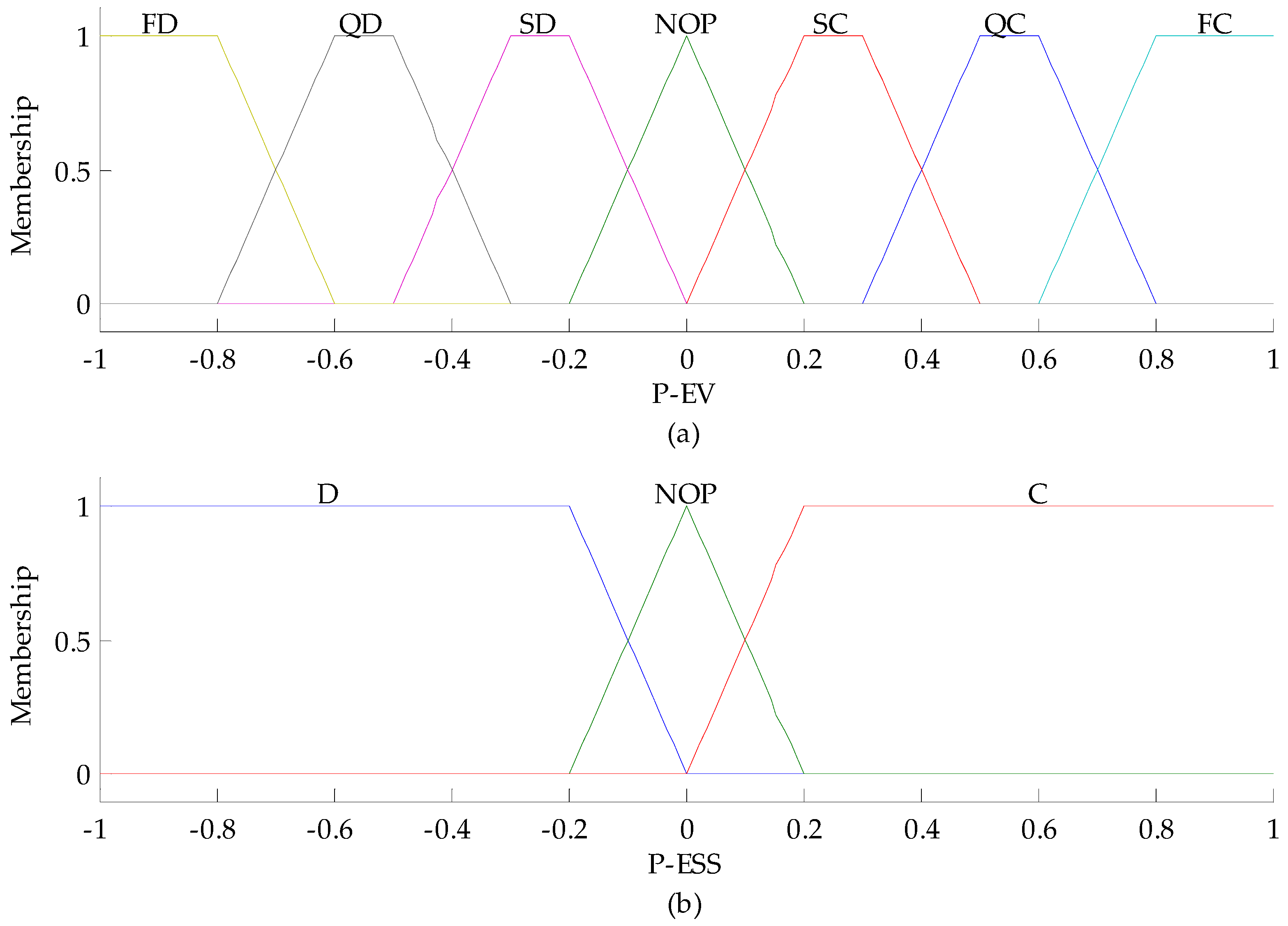
3.3.4. Fuzzy Membership Rule

In this method, considering that each objective has a specified value at each point of the Pareto front, all points are ranked based on their overall Fuzzy membership value ${\gamma }^p$ and point with the highest ${\gamma }^p$ is considered the best answer. We have:

$${\gamma }_r^p=\frac{f_r^{max}-f_r}{f_r^{max}-f_r^{min}}$$

(43)

$${\gamma }^p=\frac{{{\displaystyle \sum }}_{r=1}^{N_{OF}}{\gamma }_r^p}{{{\displaystyle \sum }}_{p=1}^{N_{PP}}{{\displaystyle \sum }}_{r=1}^{N_{OF}}{\gamma }_r^p},$$

(44)

where ${\gamma }_r^p$ is the Fuzzy membership value of the point $p$ for the $r$th objective function, and $f_r^{max}$ and $f_r^{min}$ are respectively the maximum and minimum value of the $r$th objective function in all points of the Pareto front. $N_{OF}$ is the number of objective functions and $N_{PP}$ is the number of Pareto front points.

3.3.5. Demand Response Program

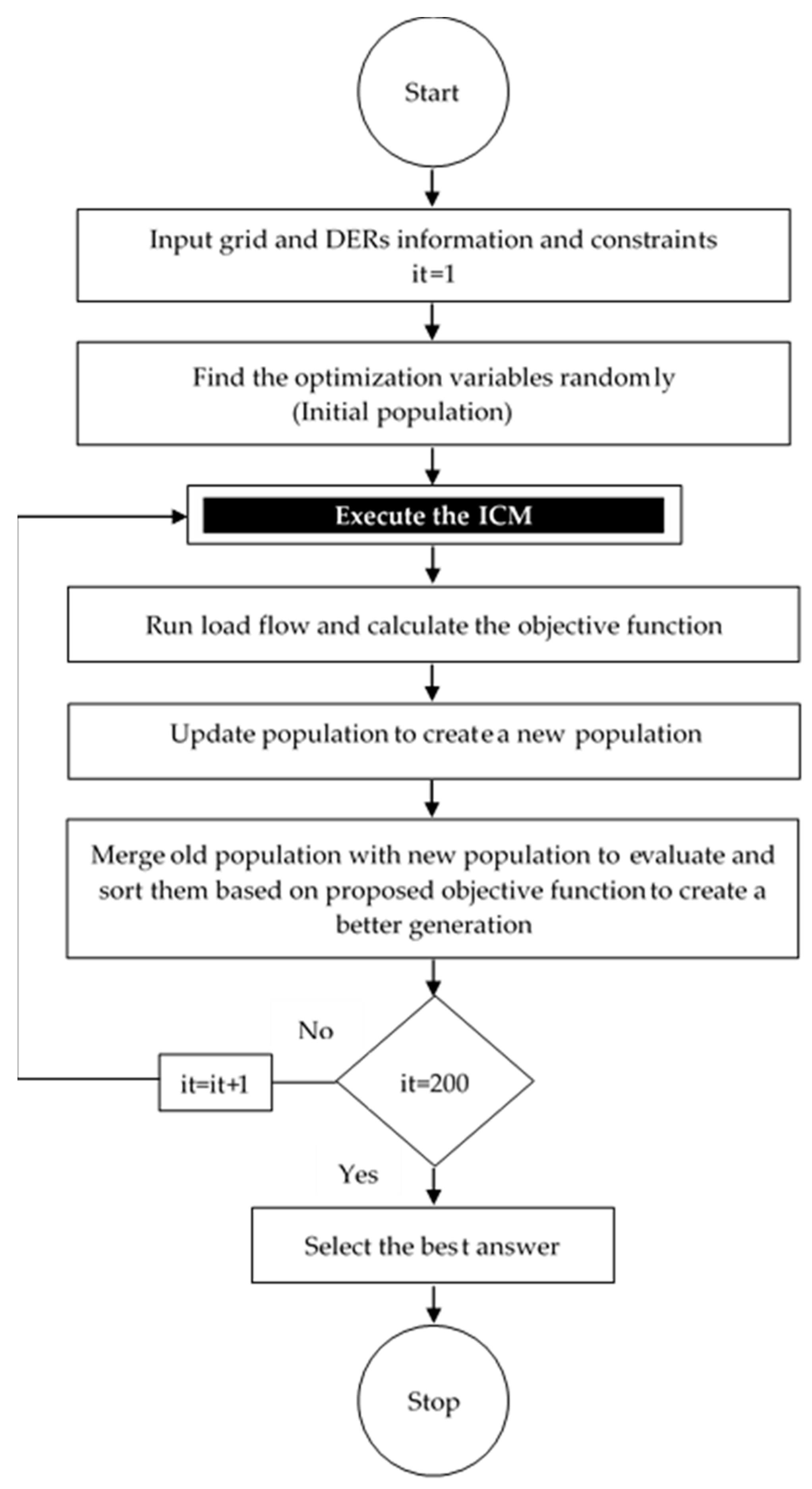
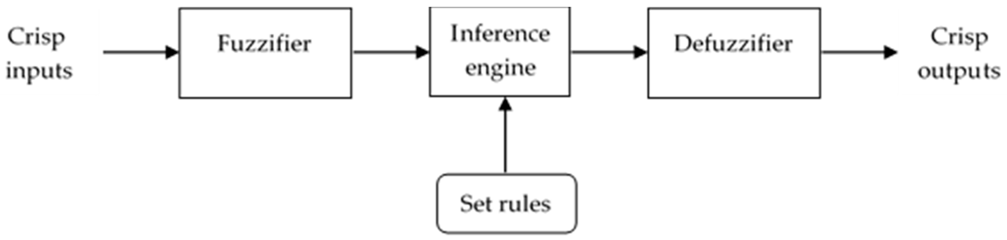
Demand response is one of the new developments in the field of demand-side management, which means consumer participation in improving the energy consumption pattern in smart grids [39]. Demand response can be divided into two general categories of time-of-use pricing (TOU) and incentive-based (IB) programs based on how consumers participate in changing their demand. In TOU, this partnership is in response to changes in electricity prices which can reduce costs and increase energy efficiency considerably. In this study, we use a TOU-based linear model to examine how customers operate in response to optimal electricity pricing [40]:

$$P_{D,i}\left(t\right)=P_{D0,i}\left(t\right)\left\{1+ϵ\left(t,t\right)\frac{\left[{\pi }^{\mathrm{TOU}}\left(t\right)-\pi \left(t\right)\right]}{\pi \left(t\right)}+{\displaystyle \sum }_{\begin{array}{c}h=1\\ h\ne t\end{array}}^{24}ϵ\left(t,h\right)\frac{\left[{\pi }^{\mathrm{TOU}}\left(h\right)-\pi \left(h\right)\right]}{\pi \left(h\right)}\right\},$$

(45)

where, $ϵ\left(t,t\right)$ and $ϵ\left(t,h\right)$ are self and cross-price elasticity of the demand which are supposed to be −0.1 and 0.001, respectively, and $\pi \left(t\right)$ is the initial hourly energy price extracted from [41]. Since we have considered two types of domestic and industrial loads, it is not sensible to assign equal elasticities for them. So, their elasticity is defined based on their importance:

$$\{\begin{array}{c}{ϵ}_{IMP}\left(t,t\right)=\left(1-IMP\right)\times ϵ\left(t,t\right)\\ {ϵ}_{IMP}\left(t,h\right)=\left(1-IMP\right)\times ϵ\left(t,h\right)\end{array}.$$

(46)

$IMP$ is the parameter assigned to the domestic and industrial loads considering their importance, which is shown in

Table 4. Loads and their importance value.

Load Type	IMP
Domestic	0.1
Industrial	0.5

. So, the modified equation is given as follow:

$$P_{D,i}\left(t\right)=P_{D0,i}\left(t\right)\left\{1+{ϵ}_{IMP}\left(t,t\right)\frac{\left[{\pi }^{\mathrm{TOU}}\left(t\right)-\pi \left(t\right)\right]}{\pi \left(t\right)}+{\displaystyle \sum }_{\begin{array}{c}h=1\\ h\ne i\end{array}}^{24}{ϵ}_{IMP}\left(t,h\right)\frac{\left[{\pi }^{\mathrm{TOU}}\left(h\right)-\pi \left(h\right)\right]}{\pi \left(h\right)}\right\}.$$

(47)

3.3.6. ICM

Optimally scheduled ESS and EVs not only improve the power quality and voltage stability but also can mitigate the negative effects of the stochastic output of RESs. To this end, the ICM which is a Mamdani-type fuzzy inference system is applied to obtain the best charging and discharging model for ESS and EVs using input information (the price of electricity, EVs and ESS state of charge, and calculated remaining load). The capability of the fuzzy inference system to handle lots of uncertainties guarantees the optimal scheduling of all EVs and ESS charging and discharging program. Figure 2 shows the architecture of the fuzzy inference system involves four main steps.

Set Rules

Here, the rules and conditions required to control the decision-making process are specified as (if…then) scenarios. These rules help the decision-making system to determine whether EVs and ESS should be charged or discharged. The fuzzy rules are shown in

Table 5. Fuzzy set rules to obtain EVs and ESS charging/discharging pattern.

INP-1	$\mathit{S}\mathit{O}{\mathit{C}}_{\mathbf{ESS}}$	VL	VL	VL	VL	VL	VL	VL	VL	VL
INP-2	$SO{C}_{\mathrm{EV}}$	VL	VL	VL	VL	VL	VL	VL	VL	VL
INP-3	CRL	L	L	L	M	M	M	H	H	H
INP-4	TUP	L	M	H	L	M	H	L	M	H
OUT-1	ESS C/D	C	C	C	C	C	C	C	C	C
OUT-2	EV C/D	FC	FC	FC	FC	QC	QC	FC	QC	SC
INP-1	$SO{C}_{\mathrm{ESS}}$	L	L	L	L	L	L	L	L	L
INP-2	$SO{C}_{\mathrm{EV}}$	L	L	L	L	L	L	L	L	L
INP-3	CRL	L	L	L	M	M	M	H	H	H
INP-4	TUP	L	M	H	L	M	H	L	M	H
OUT-1	ESS C/D	C	C	C	C	C	NOP	C	C	NOP
OUT-2	EV C/D	FC	QC	QC	QC	SC	NOP	QC	SC	NOP
INP-1	$SO{C}_{\mathrm{ESS}}$	M	M	M	M	M	M	M	M	M
INP-2	$SO{C}_{\mathrm{EV}}$	M	M	M	M	M	M	M	M	M
INP-3	CRL	L	L	L	M	M	M	H	H	H
INP-4	TUP	L	M	H	L	M	H	L	M	H
OUT-1	ESS C/D	C	C	D	C	NOP	SD	NOP	D	D
OUT-2	EV C/D	SC	SC	SD	SC	NOP	SD	NOP	SD	QD
INP-1	$SO{C}_{\mathrm{ESS}}$	H	H	H	H	H	H	H	H	H
INP-2	$SO{C}_{\mathrm{EV}}$	H	H	H	H	H	H	H	H	H
INP-3	CRL	L	L	L	M	M	M	H	H	H
INP-4	TUP	L	M	H	L	M	H	L	M	H
OUT-1	ESS C/D	NOP	D	D	D	D	D	D	D	D
OUT-2	EV C/D	NOP	SD	QD	QD	QD	FD	QD	FD	FD

.

Fuzzifier

The Fuzzifier is responsible for converting the crisp inputs into linguistic variables by using membership functions. This means that the numbers and data that need to be processed will be converted into fuzzy sets and numbers, and prepared for processing based on fuzzy logic. There are different types of fuzzy membership functions, such as the Gaussian function, triangular function, or trapezoidal function, that can be used to convert inputs into fuzzy sets. Here, we applied the trapezoidal function as it is shown in Figure 3 for the normalized input variables:

Inference Engine

The inference engine is responsible to compute the extent of Fuzzy inputs’ compliance with the IF-THEN set rules to generate the fuzzy outputs. The rate of compliance is a number between zero and one. one means complete compliance and zero means complete incompatibility. Thus, based on the calculated compliance percentage, the aggregated fuzzy outputs are made and sent to the defuzzification step to turn into crisp outputs that define the charging and discharging model of EVs and ESS.

Defuzzifier

At this stage, the outputs of the fuzzy inference engine, which are fuzzy sets, are transformed into crisp output signals of EVs and ESS charging or discharging. In this study, the center of mass method is used for the defuzzification process. Figure 4 shows the membership function of the output variables.

3.3.7. Backward-Forward Sweep Power Flow

This method is a repetition-based approach that makes use of the simple KVL (Kirchhoff’s voltage law) and KCL (Kirchhoff’s circuit law) rules [42] to obtain the parameters of power systems. In general, it has two stages that are presented separately below:

Backward sweep:

• Calculating the apparent power for each bus based on the input parameters;
• Calculating the current of each bus using Equation (48), assuming that the voltage and phase angle at each bus is equal to one and zero, respectively;

  $$I_i={\left(S_i/V_i\right)}^{*}.$$

  (48)
• Calculating the line currents based on Equation (49) considering the values obtained for the current of each bus moving from the end nodes to the slack bus:

  $$I_{\left(i,i-1\right)}=I_i+{{\displaystyle \sum }}^{}currentsinbranchesemanatingfrombusnumber\left(i\right).$$

  (49)

Forward sweep:

• Calculating the bus voltages according to Equation (50), taking into account the voltage drop moving from the first bus to the last bus. It has to be mentioned that for 1st bus as it is a slack bus, the voltage magnitude and phase angle are considered to be one and zero, respectively:

  $$V_i=V_{i-1}+I_{\left(i-1,i\right)}\times Z_{\left(i-1,i\right)}.$$

  (50)
• Controlling the convergence criteria (continue if the difference between the newly calculated value for the voltage amount and the previous one is higher than the convergence condition. Otherwise, stop the load flow calculation);
• Calculating the bus currents using new values obtained for the bus voltages;
• Return to the first step of the backward sweep stage.

4. Results and Discussion

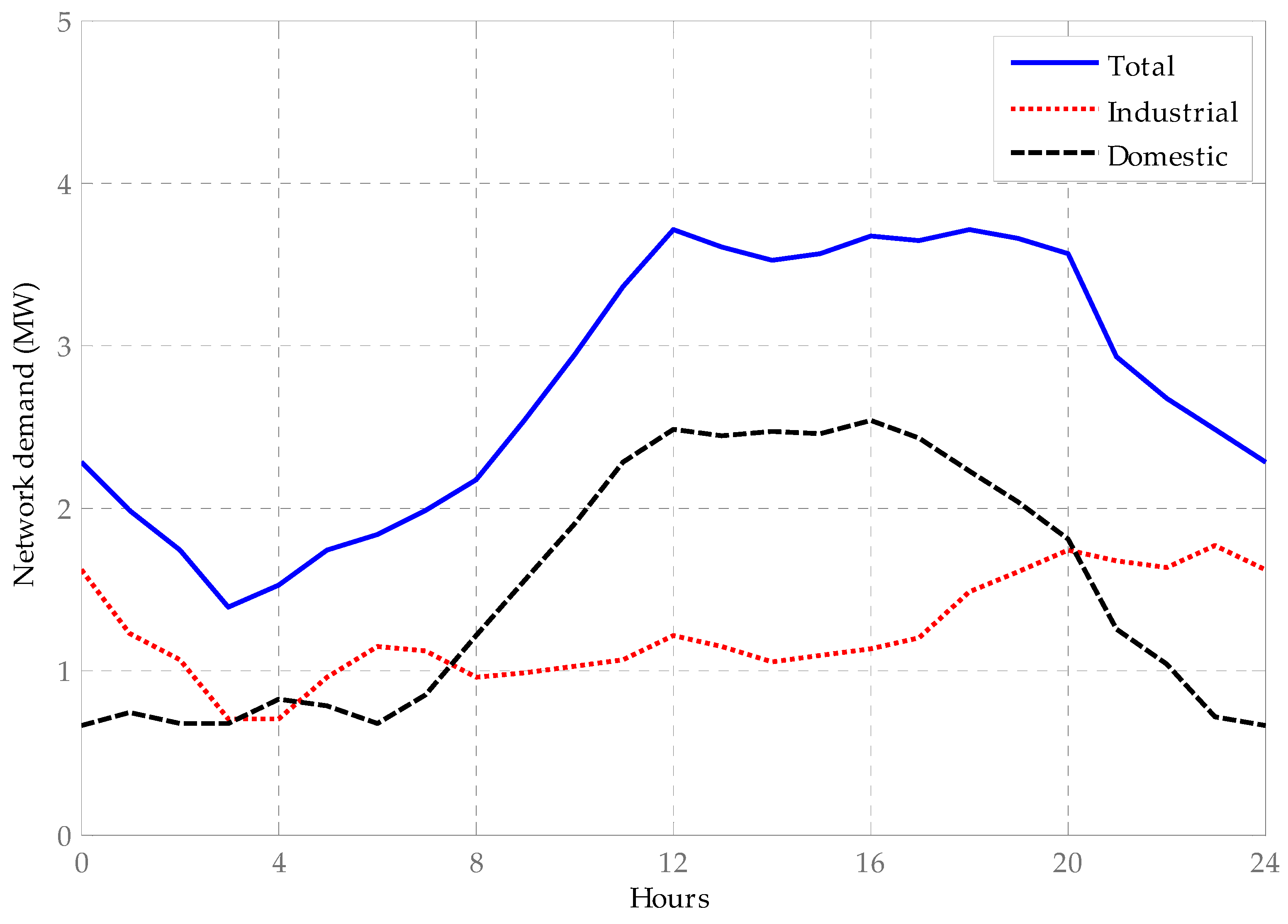
Sample Case Study

In this paper, the proposed algorithm has been tested on the IEEE-33 bus network which it’s single line diagram is adapted from [28] and shown in Figure 5. Accordingly, the electricity supply is just carried out by the centralized power plant connected to bus 1. Simulations are performed in eight different scenarios, briefly summarized in

Table 6. Description of the conducted scenarios.

Scenario	Description	Scenario	Description
1	Base case	2	Only RES
3	Only ESS	4	RES and ESS
5	Only parking lot	6	RES and Parking lot
7	ESS and Parking lot	8	RES and ESS and Parking lot

. The results of our studies are presented below:

According to the base case-load profile (Ontario- February 16, 2018) [43] Figure 6, the network demand is composed of two types of domestic and industrial customers. Regarding the total system demand, despite falling sharply, it then increased to its peak (3.715 MW) at 12:00. It then experienced a period of volatility for the next 8 hours and then decreased considerably until 24:00. The figure for domestic customers fluctuated over the first 6 hours and grew significantly until 12:00, entered a period of fluctuation at about 2.5 MW from 12:00 to 16:00. Afterward, the numbers decreased sharply to under 1 MW at 24:00. Industrial section consumption pattern started from 1.796 MW, then the figure decreased to 0.859 MW at 4:00. From this point to 8:00 the consumption rate increased and experienced a period of volatility by the hour 16:00. From this point onwards, the trend increased continuously. As for network peak hours (12:00–20:00), domestic and industrial sections, have made up 64.4% and 36.6% of the total system demand, respectively.

Table 7. Obtained values for target variables through optimization process.

Target Variables	1	2	3	4	5	6	7	8
PV loc.	−	29	−	12	−	33	−	12
PV cap.	−	715.26	−	603.99	−	868.19		704.5
Wind loc.	−	11	−	31	−	22		29
Wind cap.	−	956.26	−	1196.01	−	1108.72	−	1308.4
ESS loc.	−	−	11 24	25 22	−	−	10 31	10 25
ESS cap.	−	−	350.04 271.88	314.62 388.27	−	−	295.65 403.04	375 625
Parking loc.	−	−	−	−	6 30	23 12	22 25	4 27
Parking cap.	−	−	−	−	847.91 515.37	881.26 1004.79	756.21 843.79	1200.32 1254.58

shows the optimal location and capacity of DERs obtained from the GA-PSO for different scenarios. As it is obvious, the simultaneous presence of RESs and ESSs have provided conditions to increase the EVs penetration to the network. This development is occurred when the voltage deviation has not increased, resulting in cost saving. According to

Table 8. Obtained values for objective functions.

Scenario	Processing Time (sec)	${\mathit{f}}_1\left(\mathbf{M}\mathbf{W}\right)$	${\mathit{f}}_2\left(\mathbf{p}\mathbf{u}\right)$	${\mathit{f}}_3\left(\mathbf{\$}\right)$
1	82	4.04	38.05	16,431,256.00
2	149	3.01	29.2	09,416,752.81
3	125	3.75	36.98	16,209,434.04
4	199	2.79	27.77	08,743,071.31
5	187	3.27	34.16	16,027,047.10
6	263	2.44	24.99	07,952,727.90
7	240	3.35	33.67	15,843,017.04
8	317	1.98	22.54	07,360,217.66

, the combined utilization of DERs and the implementation of the ICM have led to increased computation time. This is because of the complexity of the system imposed by the uncertainties from EV, ESS, and RES models. Accordingly, the presence of EV modeling in simulations has by far increased the processing time more than the two others, due to the consideration of probabilistic factors such as their mileage, arrival or departure time and their SOC in EV modeling. RES has the second-highest impact on processing time, followed by ESS so that they have increased the computation time by 67 and 43 seconds, respectively, compared to the time for the base case. As for technical issues, the simultaneous presence of ESSs and EV parking lots has enabled the production of RESs to be distributed through different hours, so the power losses and voltage deviations are decreased. Furthermore, considering EV as a controllable load and applying demand response program resulted in a further reduction in costs, losses, and voltage deviation. So, in scenario 8, with the combined utilization of DERs and scheduled charging and discharging of ESS and EVs, the $f_1$, $f_2$ and $f_3$ are improved with an amount of 51%, 40.77%, and 55.21%, respectively, compared to the base case. The network demand curve for scenario 8 is shown in Figure 7:

Figure 8 gives the hourly network operational strategy along with the network demand profile in scenario 8. According to Figure 8, the highest system demand occurred at 12:00, in which 54.3% of its amount is provided by resources other than the centralized power plant. Thus, there is not only a great reduction in system dependency on the centralized power plant but also a suitable condition to decrease the network operation costs in peak hours. As it is obvious, EV charging has been carried out in the time-period of 22:00–09:00, which is the network’s low load hours and low energy prices according to the ICM. On the contrary, EVs are discharged in the time-period of 10:00–21:00, which is the peak of network consumption with high energy prices. This process has been done according to the ICM for more profitability for car owners. Consequently, in comparison with Figure 7, the difference between the maximum and minimum value for each trend in Figure 7 has been decreased, which considerably moderates the demand curve.

The share of each resource in supplying the total system demand for 24-hours is presented in

Table 9. The contribution of each resource in supplying total 24-hour electrical demand.

Demand Supplied by Other Resources (%)
Scenario	Total System Load (MW)	RES	V2G	ESS	CPP (%)
1	66.280	−	−	−	100
2	66.280	40.65	−	−	59.35
3	67.190	−	−	1.27	98.73
4	67.309	43.57	−	1.44	54.99
5	68.133	−	2.46	−	97.54
6	68.166	47.91	2.50	−	49.59
7	68.902	−	2.10	1.39	96.51
8	70.238	49.27	3.42	1.63	45.68

. The results highlight the potency of our proposed method to decrease the share of the centralized power plant in demand supplying.

According to Table 9, the deployment of EVs and ESSs to the network resulted in an increased share of RESs in supplying the customers’ demand. So, the reduction in dependency on centralized power will reduce the DSO’s costs and increase its profit,

Table 10. Distribution network operators (DSO) profit.

Scenario	Total DSO Profit ($)	Peak Hours Profit ($)	Low Load Hours Profit ($)
2	6,926,503.47	3,869,185.11	3,057,318.36
3	0311,911.95	0276,199.37	0035,712.58
4	7,185,884.93	4791,212.64	3,946,720.29
5	0394,297.27	0244,049.55	0150,247.72
6	8,378,418.19	5,570,857.10	2,807,561.09
7	0683,438.52	0295,294.17	0388,144.35
8	9,071,038.34	6,170,581.26	2,900,457.08

. In particular, there is no longer a need to purchase all the required power from the centralized power plant to supply demand, especially during peak hours.

As for Table 10, overall, RESs had by far the greatest impact on DSO’s profit. As it is clear, in scenarios 2, 4 and 6 DSO experienced high incomes where the RESs were utilized to supply customers. Results justify the uncertainties in RESs production. Furthermore, EVs with V2G capability came in second place given their impact on DSO’s profit. The third effective factor, ESSs, had a negligible effect on DSO’s profit because they had a lower contribution in power supplying compare to the two others.

Obtaining optimum location and size of DERs and scheduling ESS and EVs operation have influenced the power system parameters, e.g., the bus voltages are improved. Figure 9 gives the average voltage magnitude for each bus over a 24-hour time. Accordingly, the maximum deviation from the desired value of 1 per-unit for each bus has occurred in the base case scenario, in the absence of DERs. With respect to bus number 33, the farthest point from the centralized power plant, the best number is reported in scenario 8 due to the integration of DERs in the grid. Regarding total deviation, the smallest enhancement can be seen in the third scenario. This is because the capacity of ESS is limited and these devices are considered as spinning reserve, not voltage regulators. So, to achieve the best result, the combination of RESs, ESSs, and EV parking lots along with the implementation of the ICM (scenario 8) is the best scenario.

Furthermore, to independently study the effect of time of use pricing on system operation, Figure 10 compares statistics regarding hourly system demand extracted from the base case, scenario 8 with fixed pricing, and scenario 8 with the time of use pricing method. Generally, it can be seen that, as the demand response program is implemented, a part of customers has reduced their consumption and also shifted part of their demand to low load hours.

Table 11. Network operational indicators.

Scenario	Total System Loss (MW)	Total System Load (MW)	Peak Shaving (MW)	Peak to Valley Distance (MW)	Load Factor (%)
Base case	4.04	66.280	−	2.326	85.1
Fixed pricing	2.11	70.238	−0.1	1.997	88.5
Online pricing	1.98	65.248	0.295	1.506	90.2

provides detailed information regarding Figure 10:

Overall, as it is clear, all technical indicators are improved after applying demand-side management program. Therefore, it ensures the reliable operation of the system and also increases the system operating efficiency.

In order to investigate the effectiveness of the proposed algorithm,

Table 12. Comparison of the proposed genetic algorithm (GA)-particle swarm optimization (PSO) algorithm with literature (scenario 8).

Algorithm	Iteration	Pop Size	NOFE	Processing Time (sec)	${\mathit{f}}_1\left(\mathbf{MW}\right)$	${\mathit{f}}_2\left(\mathbf{pu}\right)$	${\mathit{f}}_3\left(\mathbf{\$}\right)$
Adaptive GA-PSO	200	50	72,480	317	1.98	22.54	07,360,217.66
NSGA-II	200	50	99,667	436	3.00	23.81	10,109,490.86
DE	200	50	83,516	374	−	−	−
GA	200	50	96,860	428	−	−	−
E-PSO	200	50	114,127	495	2.09	22.90	07,582,571.10

provides a comparison between our proposed method with some other algorithms provided by literature to deal with the case defined in scenario 8. In order to compare the computation speed, the number of function evaluation (NOFE) index is defined, in which the lower number of NOFE, the higher speed of the algorithm.

Overall, it can be seen that GA-PSO in the same condition has operated faster and more accurately than the four others. because of the large number of variables in the problem, DE and GA algorithms did not converge to the final answer. The NSGA-II algorithm, despite its good performance at the beginning of the process, did not end up at the optimal value at the end of the permissible number of iterations. Although the final answer of both GA-PSO and E-PSO algorithms is almost close to each other, the faster operation of GA-PSO makes it the better choice.

5. Conclusions

Distributed energy resources will be an integral part of future power systems and play a great technical role and bring many financial benefits. In this paper, the benefits of DERs were considered to facilitate their integration into microgrids to meet the extra demand load in the most possible economical, effective, and reliable manner. To this end, a novel two-layer model was proposed to minimize the multi-objective optimization problem consists of three techno-economical parts: power losses, voltage fluctuations, and demand supplying costs. Through the outer layer, the simultaneous determination of the optimal capacity and location of DERs is accomplished based on the probabilistic models. The inner layer corresponds to schedule the charging and discharging of EVs and ESSs by using the fuzzy logic-based ICM. The formulated objective function is solved by using the GA-PSO algorithm and the Fuzzy membership-based approach is applied to derive the optimal solution from the Pareto frontier. To show the efficacy of the proposed model, the results from an IEEE 33-bus network in eight different scenarios were presented and discussed.

The given results indicated that optimized penetration of DERs into the distribution network improves the system operation indices (e.g., voltage deviation in sensitive buses). Applying the ICM to schedule the EVs and ESSs charging, has decreased the voltage fluctuations and power losses dramatically. The proposed method also enabled new functionalities for RESs, e.g., they can operate as distributed generators. This feature gives RESs the ability to supply more demand for the network along with the needs of EV batteries, which can greatly decrease the costs for DSO and customers as well. Furthermore, the proposed demand-side management model has modified the network demand curve and reduced costs significantly. Further, the utilization of the proposed Fuzzy membership-based method for solving the optimization problem resulted in a more accurate and efficient answer compare to other solving methods.

Future works can focus on the deployment of various DERs in microgrids. As we proposed a comprehensive model that optimizes energy management in smart grids with non-conventional energy resources integration, hourly updated information of uncertainties can be deployed to increase the accuracy of the proposed model. Further, the effects of different DERs, such as micro-turbines and diesel generators can be studied on the power system stability and reliability over larger time frames (weekly and yearly).

References

1. Hosseini, S.; Sarder, M. Development of a Bayesian network model for optimal site selection of electric vehicle charging station. Int. J. Electr. Power Energy Syst. 2019, 105, 110–122. [Google Scholar] [CrossRef]
2. de Melo, H.N.; Trovao, J.P.F.; Pereirinha, P.G.; Jorge, H.M.; Antunes, C.H. A controllable bidirectional battery charger for electric vehicles with vehicle-to-grid capability. IEEE Trans. Veh. Technol. 2017, 67, 114–123. [Google Scholar] [CrossRef]
3. Jacob, A.S.; Banerjee, R.; Ghosh, P.C. Sizing of hybrid energy storage system for a PV based microgrid through design space approach. Appl. Energy 2018, 212, 640–653. [Google Scholar] [CrossRef]
4. Golshannavaz, S. Cooperation of electric vehicle and energy storage in reactive power compensation: An optimal home energy management system considering PV presence. Sustain. Cities Soc. 2018, 39, 317–325. [Google Scholar] [CrossRef]
5. Shafie-Khah, M.; Heydarian-Forushani, E.; Golshan, M.; Siano, P.; Moghaddam, M.; Sheikh-El-Eslami, M.; Catalão, J. Optimal trading of plug-in electric vehicle aggregation agents in a market environment for sustainability. Appl. Energy 2016, 162, 601–612. [Google Scholar] [CrossRef]
6. Yang, F.; Feng, X.; Li, Z. Advanced microgrid energy management system for future sustainable and resilient power grid. IEEE Trans. Ind. Appl. 2019, 55, 7251–7260. [Google Scholar] [CrossRef]
7. Dou, C.; An, X.; Yue, D.; Li, F. Two-level decentralized optimization power dispatch control strategies for an islanded microgrid without communication network. Int. Trans. Electr. Energy Syst. 2017, 27, e2244. [Google Scholar] [CrossRef]
8. Faddel, S.; Elsayed, A.T.; Mohammed, O.A. Bilayer multi-objective optimal allocation and sizing of electric vehicle parking garage. IEEE Trans. Ind. Appl. 2018, 54, 1992–2001. [Google Scholar] [CrossRef]
9. Marzband, M.; Alavi, H.; Ghazimirsaeid, S.S.; Uppal, H.; Fernando, T. Optimal energy management system based on stochastic approach for a home Microgrid with integrated responsive load demand and energy storage. Sustain. Cities Soc. 2017, 28, 256–264. [Google Scholar] [CrossRef]
10. Amini, M.H.; Karabasoglu, O. Optimal operation of interdependent power systems and electrified transportation networks. Energies 2018, 11, 196. [Google Scholar] [CrossRef] [Green Version]
11. Gonçalves, J.; Martins, A.; Neves, L. Methodology for real impact assessment of the best location of distributed electric energy storage. Sustain. Cities Soc. 2016, 26, 531–542. [Google Scholar] [CrossRef] [Green Version]
12. Fan, S.; Ai, Q.; Piao, L. Hierarchical energy management of microgrids including storage and demand response. Energies 2018, 11, 1111. [Google Scholar] [CrossRef] [Green Version]
13. Maulik, A.; Das, D. Optimal power dispatch considering load and renewable generation uncertainties in an AC–DC hybrid microgrid. IET Gener. Transm. Distrib. 2019, 13, 1164–1176. [Google Scholar] [CrossRef]
14. Atia, R.; Yamada, N. Sizing and analysis of renewable energy and battery systems in residential microgrids. IEEE Trans. Smart Grid 2016, 7, 1204–1213. [Google Scholar] [CrossRef]
15. Amini, M.H.; McNamara, P.; Weng, P.; Karabasoglu, O.; Xu, Y. Hierarchical electric vehicle charging aggregator strategy using Dantzig-Wolfe decomposition. IEEE Des. Test 2017, 35, 25–36. [Google Scholar] [CrossRef]
16. Liu, R.-S.; Hsu, Y.-F. A scalable and robust approach to demand side management for smart grids with uncertain renewable power generation and bi-directional energy trading. Int. J. Electr. Power Energy Syst. 2018, 97, 396–407. [Google Scholar] [CrossRef]
17. Moradi, H.; Esfahanian, M.; Abtahi, A.; Zilouchian, A. Optimization and energy management of a standalone hybrid microgrid in the presence of battery storage system. Energy 2018, 147, 226–238. [Google Scholar] [CrossRef]
18. Asgher, U.; Babar Rasheed, M.; Al-Sumaiti, A.S.; Ur-Rahman, A.; Ali, I.; Alzaidi, A.; Alamri, A. Smart energy optimization using heuristic algorithm in smart grid with integration of solar energy sources. Energies 2018, 11, 3494. [Google Scholar] [CrossRef] [Green Version]
19. Rahbari, O.; Vafaeipour, M.; Omar, N.; Rosen, M.A.; Hegazy, O.; Timmermans, J.-M.; Heibati, S.; Van Den Bossche, P. An optimal versatile control approach for plug-in electric vehicles to integrate renewable energy sources and smart grids. Energy 2017, 134, 1053–1067. [Google Scholar] [CrossRef]
20. Khalid, Z.; Abbas, G.; Awais, M.; Alquthami, T.; Rasheed, M.B. A Novel Load Scheduling Mechanism Using Artificial Neural Network Based Customer Profiles in Smart Grid. Energies 2020, 13, 1062. [Google Scholar] [CrossRef] [Green Version]
21. Moradi, M.H.; Abedini, M.; Tousi, S.R.; Hosseinian, S.M. Optimal siting and sizing of renewable energy sources and charging stations simultaneously based on Differential Evolution algorithm. Int. J. Electr. Power Energy Syst. 2015, 73, 1015–1024. [Google Scholar] [CrossRef]
22. Mozafar, M.R.; Moradi, M.H.; Amini, M.H. A simultaneous approach for optimal allocation of renewable energy sources and electric vehicle charging stations in smart grids based on improved GA-PSO algorithm. Sustain. Cities Soc. 2017, 32, 627–637. [Google Scholar] [CrossRef]
23. Abedini, M.; Moradi, M.H.; Hosseinian, S.M. Optimal management of microgrids including renewable energy scources using GPSO-GM algorithm. Renew. Energy 2016, 90, 430–439. [Google Scholar] [CrossRef]
24. Rahmani-Andebili, M.; Shen, H.; Fotuhi-Firuzabad, M. Planning and operation of parking lots considering system, traffic, and drivers behavioral model. IEEE Trans. Syst. Man Cybern. Syst. 2018, 49, 1879–1892. [Google Scholar] [CrossRef]
25. Grande, L.S.A.; Yahyaoui, I.; Gómez, S.A. Energetic, economic and environmental viability of off-grid PV-BESS for charging electric vehicles: Case study of Spain. Sustain. Cities Soc. 2018, 37, 519–529. [Google Scholar] [CrossRef]
26. Domínguez-Navarro, J.; Dufo-López, R.; Yusta-Loyo, J.; Artal-Sevil, J.; Bernal-Agustín, J. Design of an electric vehicle fast-charging station with integration of renewable energy and storage systems. Int. J. Electr. Power Energy Syst. 2019, 105, 46–58. [Google Scholar] [CrossRef]
27. Kayal, P.; Chanda, C. Optimal mix of solar and wind distributed generations considering performance improvement of electrical distribution network. Renew. Energy 2015, 75, 173–186. [Google Scholar] [CrossRef]
28. Delfino, F.; Ferro, G.; Minciardi, R.; Robba, M.; Rossi, M.; Rossi, M. Identification and optimal control of an electrical storage system for microgrids with renewables. Sustain. Energy Grids Netw. 2019, 17, 100183. [Google Scholar] [CrossRef]
29. Jarraya, I.; Masmoudi, F.; Chabchoub, M.H.; Trabelsi, H. An online state of charge estimation for Lithium-ion and supercapacitor in hybrid electric drive vehicle. J. Energy Storage 2019, 26, 100946. [Google Scholar] [CrossRef]
30. Amini, M.; Moghaddam, M.P. Probabilistic modelling of electric vehicles’ parking lots charging demand. In Proceedings of the 2013 21st Iranian Conference on Electrical Engineering (ICEE), Mashhad, Iran, 14–16 May 2013; pp. 1–4. [Google Scholar]
31. Mozafar, M.R.; Amini, M.H.; Moradi, M.H. Innovative appraisement of smart grid operation considering large-scale integration of electric vehicles enabling V2G and G2V systems. Electric Power Syst. Res. 2018, 154, 245–256. [Google Scholar] [CrossRef]
32. Domínguez-García, A.; Heydt, G.; Suryanarayanan, S. Implications of the smart grid initiative on distribution engineering (final project report-part2). PSERC Doc. 2011, 11–50. Available online: https://pserc.wisc.edu/document_search.aspx (accessed on 20 February 2017).
33. Meliopoulos, S.; Meiselrge, J.; Overbye, T. Power system level impacts of plug-In hybrid vehicles (final project report). PSERC Doc. 2009, 14–38. Available online: https://pserc.wisc.edu/document_search.aspx (accessed on 20 February 2017).
34. Pasaoglu, G.; Fiorello, D.; Martino, A.; Scarcella, G.; Alemanno, A.; Zubaryeva, A.; Thiel, C. Driving and parking patterns of European car drivers-a mobility survey. Luxemb. Eur. Comm. Joint Res. Centre 2012. Available online: https://ec.europa.eu/jrc/en/publication/eur-scientific-and-technical-research-reports/driving-and-parking-patterns-european-car-drivers-mobility-survey (accessed on 18 May 2017).
35. Pasaoglu, G.; Fiorello, D.; Zani, L.; Martino, A.; Zubaryeva, A.; Thiel, C. Projections for electric vehicle load profiles in Europe based on travel survey data. Joint Res. Cent. Eur. Comm. Petten Neth. 2013. Available online: https://ec.europa.eu/jrc/en/publication/eur-scientific-and-technical-research-reports/projections-electric-vehicle-load-profiles-europe-based-travel-survey-data (accessed on 18 May 2017).
36. Letendre, S.; Denholm, P.; Lilienthal, P. New load, or new resource? The industry must join a growing chorus in calling for new technology. Public Util. Fortn. 2006, 144, 28–37. [Google Scholar]
37. Beasley, D.; Bull, D.R.; Martin, R.R. An overview of genetic algorithms: Part 2, research topics. Univ. Comput. 1993, 15, 170–181. [Google Scholar]
38. Eberhart, R.C.; Shi, Y.; Kennedy, J. Swarm Intelligence (Morgan Kaufmann Series in Evolutionary Computation); Morgan Kaufmann Publishers: Burlington, MA, USA, 2001. [Google Scholar]
39. Benegiamo, A.; Loiseau, P.; Neglia, G. Dissecting demand response mechanisms: The role of consumption forecasts and personalized offers. Sustain. Energy Grids Netw. 2018, 16, 156–166. [Google Scholar] [CrossRef] [Green Version]
40. Aalami, H.; Moghaddam, M.P.; Yousefi, G. Demand response modeling considering interruptible/curtailable loads and capacity market programs. Appl. Energy 2010, 87, 243–250. [Google Scholar] [CrossRef]
41. Board, O.E. Regulated Price Plan Manual. 2005. Available online: http://www.ontla.on.ca/library/repository/mon/11000/255532.pdf (accessed on 16 May 2018).
42. Rana, A.; Darji, J.; Pandya, M. Backward/forward sweep load flow algorithm for radial distribution system. Int. J. Sci. Res. Dev. 2014, 2, 398–400. [Google Scholar]
43. H.O.E. Independent Electricity System Operator (IESO). Available online: http://reports.ieso.ca/public/DemandZonal/ (accessed on 16 May 2018).
Figure 1. Flowchart of the optimization process.
Energies 13 01706 g001
Figure 2. Fuzzy inference system architecture.
Energies 13 01706 g002
Figure 3. Membership function of input variables on the weight of (a) EV state of charge, (b) ESS state of charge, (c) calculated remaining load and (d) time-of-use price.
Energies 13 01706 g003
Figure 4. Membership function of output variables on weight of (a) EV charging/discharging power and (b) ESS charging/discharging power.
Energies 13 01706 g004
Figure 5. Single line diagram of the IEEE-33 bus network.
Energies 13 01706 g005
Figure 6. Network 24-hours electrical demand profile (scenario 1).
Energies 13 01706 g006
Figure 7. Network 24-hour electrical demand profile (scenario 8).
Energies 13 01706 g007
Figure 8. Network operational strategy in supplying electrical demand (scenario 8).
Energies 13 01706 g008
Figure 9. Voltage profile for 24-hour.
Energies 13 01706 g009
Figure 10. Network 24-hour electrical demand profile.
Energies 13 01706 g010