Short-Term Photovoltaic Power Forecasting Using a Convolutional Neural Network–Salp Swarm Algorithm


1
Department of Electrical Engineering, National Cheng Kung University, Tainan 70101, Taiwan
2
Department of Industrial and Process Engineering, Kalimantan Institute of Technology, Balikpapan, East Kalimantan, Timur 76127, Indonesia
3
Department of Electrical Engineering, Kun Shan University, Tainan 70101, Taiwan
*
Author to whom correspondence should be addressed.
Energies 2020, 13(8), 1879; https://0-doi-org.brum.beds.ac.uk/10.3390/en13081879
Submission received: 15 March 2020
/
Revised: 8 April 2020
/
Accepted: 8 April 2020
/
Published: 12 April 2020
(This article belongs to the Special Issue Machine Learning and Optimization with Applications of Power System II)
Abstract
:The high utilization of renewable energy to manage climate change and provide green energy requires short-term photovoltaic (PV) power forecasting. In this paper, a novel forecasting strategy that combines a convolutional neural network (CNN) and a salp swarm algorithm (SSA) is proposed to forecast PV power output. First, the historical PV power data and associated weather information are classified into five weather types, such as rainy, heavy cloudy, cloudy, light cloudy and sunny. The CNN classification is then used to determine the prediction for the next day’s weather type. Five models of CNN regression are established to accommodate the prediction for different weather types. Each CNN regression is optimized using a salp swarm algorithm (SSA) to tune the best parameter. To evaluate the performance of the proposed method, comparisons were made to the SSA based support vector machine (SVM-SSA) and long short-term memory neural network (LSTM-SSA) methods. The proposed method was tested on a PV power generation system with a 500 kWp capacity located in south Taiwan. The results showed that the proposed CNN-SSA could accommodate the actual generation pattern better than the SVM-SSA and LSTM-SSA methods.
1. Introduction
As photovoltaic (PV) power harvesting becomes more affordable, PV systems are increasingly being integrated into and used for existing power systems. For example, PV power is used in reactive power planning [1], energy storage systems (ESSs) [2], and various billing mechanisms in demand-side management [3]. Techno-economic evaluation was conducted in Gao et al. [4]. PV power systems are more accessible to the demand side but create new problems due to their variability, particularly in larger PV power systems. In Mills and Wiser [5], short-term power forecasting was used to determine the balancing reserve from renewables. The forecasting algorithm accuracy determines the solar variability, which significantly increases the cost.
In Zhang et al. [6], PV power injection reduces the costs of the spinning reserve more than the improved unit commitment and economic dispatch do. The paper also emphasizes that some forecasting errors must be managed and that these increase as the plant size increases. In Yang and Liao [7], the optimal PV reactive power regulation was researched, whereby accurate PV power forecasting leads to more reactive power regulation. In Di Piazza et al. [8], the online replanning task was used to minimize the maximum deviation due to forecasting errors for the PV-ESS hybrid system in reshaping the daily grid-injected power profile. In Nguyen et al. [9], the optimal power flow in the multiphase distribution system was used to accommodate high PV power penetration. Research indicates that reliable forecasting accuracy for PV power harvesting is required to determine the operation of existing power systems less problematically through the mass integration of PV power systems.
PV power forecasting has been researched widely by using statistical analysis, machine learning, and deep learning methods. In De Giorgi et al. [10], multiple linear regression was used to forecast the PV power output, in which the input variables were the historical PV output, module temperature, ambient temperature, and solar irradiance. In recent years, machine-learning-based forecasting methods, such as artificial neural networks (ANNs) [11] and support vector machines (SVMs) [12], have gained popularity because of their ability to capture abrupt changes in the input–output relationship due to variable environmental conditions. Various ANN models are used for day-ahead PV forecasting algorithms. In Mellit et al. [13], an adaptive feedforward backpropagation neural network was employed as the short-term power forecasting algorithm, which used solar irradiance, cell temperature, and historical power output on three typical days, including sunny, partially cloudy, and overcast days.
In Dolara et al. [14], a hybrid ANN and clear sky solar radiation model was developed by using input variables from a weather forecast provider and a clear-sky radiation model (CSRM) curve for physical weather input. This paper emphasizes that weather information is required, although one peculiar weather condition caused huge errors. In Nespoli et al. [15], a multilayer perceptron ANN combined with CSRM was used to forecast sunny and cloudy days. In Zeng and Qiao [16], an SVM was developed using 14 years of historical data and using several preconditions for historical data as input variables, namely the latest observed solar radiation, radiation at the hour of forecasting in the previous two consecutive days, and the latest observations for some meteorological features, including sky cover, wind speed, and relative humidity. In Preda et al. [17], an SVM was used as the PV power forecasting model with big data analysis. The dataset was divided into two parts for sunny days and partially sunny days. In Wang et al. [18], a recurrent neural network was used to forecast the PV output power, providing analysis for adjacent days. Preconditioning arrangements were also used for historical data: previous days, previous time of forecasting, and expected output power.
The state-of-the-art algorithms of convolutional neural networks (CNNs) and long short-term memory neural networks (LSTMs) are popular in wind power forecasting [19] and load forecasting [20]. In Han et al. [21], the CNN and LSTM permitted the incorporation of pseudoperiodicity and the long-term dependency of input variables into the prediction model. Deep learning in PV power forecasting is widely used, especially in CNNs and LSTMs, whose structure can record chronological past information and accommodate time-series sequences. In Zhang et al. [22], a variation mode decomposition CNN was developed using the daily and hourly historical input variables of temperature, wind speed, and solar radiation. The forecasting model was required to convert data points into intrinsic mode functions and residue, which formed 14 images.
In Huang and Kuo [23], a CNN-based PV power forecasting algorithm was developed by considering temperature, solar radiation, and daily and past-five-days PV power output. The CNN used three convolutional layers with kernel sizes of 9, 7, and 5, respectively, and a scaled exponential linear unit (SELU) as the activation function. In Wan et al. [24], a multivariate temporal convolutional network was constructed using three convolutional layers with kernel sizes of 24, 72, and 168 with no pooling layer. In Deng et al. [25], a multiscale CNN was developed to forecast PV power two days in advance by incorporating various scales of dilated convolutions. The input variables were arranged using a seven-day periodicity. This study inferred a gradual increase in the prediction error toward the end of a prediction window.
In Du et al. [26], a CNN-based PV power forecasting algorithm was used for a building-attached PV in China. The input variables were arranged using 15-min numerical weather prediction (NWP) with data such as direct irradiance, temperature, air quality index, relative humidity, and wind speed. Those input variables were later classified into four weather conditions: clear, partially cloudy, mostly cloudy, and rainy. In Lee et al. [27], two CNNs of different sizes were combined with LSTM to adaptively extract both long-range and short-time local features. The CNN was manually tuned with filter sizes of (2, 4), (4, 8), and (8, 16) using NWPs. In Riaz et al. [28], the fuzzy rough C-mean with an unsupervised CNN was used for the image clustering of large-scale image data. An image as input was fed into AlexNet with five convolution layers, two adjustment layers, three feature maps, a max-pooling layer, one fully connected layer, and one soft-max layer before the cluster-label production.
In Nam and Hur [29], naïve Bayes classifier and Kriging models were used to forecast the hourly uncertainty in PV power, whereby the Kriging technique allowed for the spatial modeling of weather information and the location of PV power output through the estimations of irradiance, humidity, and temperature at neighboring points. In Suresh et al. [30], a manually tuned CNN model was used for PV power forecasting, which consisted of four convolutional layers. Those convolutional layers were assigned for each input variable and fed to the max-pooling layer. The input variables consisted of irradiation, module temperature, ambient temperature, and wind speed.
In Zhao et al. [31], the use of the CNN was a time-consuming method for the time-series classification, particularly for trial-and-error CNN parameter determination. Research in Miyazaki et al. [32] offered an alternative approach to PV power forecasting by using the relationship between the movement of the geographical distribution and the harvested PV power. This approach is less practical for individual PV system users because a powerful weather station is required. In this study, an optimization tool called the salp swarm algorithm (SSA) [33] was used to tune the best parameter for the CNN.
In contrast with point forecasting, probabilistic PV power forecasting enables operators to perform flexible analyses in one plot. The worst and best conditions for prediction can be observed, which facilitates decision-making by considering the prediction uncertainty. The various probabilistic PV power forecasting methods include the modeling of random PV prediction errors with fuzzy prediction intervals [34], the modeling of PV power generation using quantile regression [35,36], and Monte Carlo simulations [37]. Moreover, random PV power generation can be related to the uncertainty of input variables modeled using a cumulant probability distribution [38]. Although probabilistic load forecasting is outside the scope of this work, the proposed method has implications for the development of probabilistic load forecasting using CNNs, which accommodates the flexible use of multivariate inputs.
Many studies [1,2,3,4,5,6,7,8,9,10,11,12,13,14,15,16,17,18,19,20,21,22,23,24,25,26,27,28,29,30,31,32,33] have identified the drawbacks of developments in PV power forecasting: (1) ineffective use of trial and error for PV power forecasting optimization; (2) extensive historical data requirements for forecasting model accuracy; (3) the requirement for temporal- and periodicity-related forecasting models to use minute fractions of NWP or any meteorological image, which are unavailable in practice for small plants; and (4) a gradual decrease in forecasting accuracy toward the end of a prediction window. Thus, this paper proposes a novel forecasting strategy to address the aforementioned problems. The proposed method uses a CNN optimized with an SSA to seamlessly generate the forecasting model without the requirement of time-consuming trial and error. The CNN classification is used for the prediction of the next day’s weather type. The CNN-SSA then produces five CNN regression models to accommodate the unique characteristics of several weather types, which are run with an hourly prediction horizon. The proposed method is compared with an optimal support vector machine and an LSTM neural network by using an SSA (SVM-SSA and LSTM-SSA).
The state-of-the-art features of the proposed method are as follows: (1) simple arrangement of input variables that moderate features and training datasets for an accurate day-ahead forecasting result, (2) a modified state-of-the-art forecasting algorithm to produce a fine-tuned CNN model that requires no time-consuming trial and error, and (3) consistent accuracy in short-term PV power forecasting from day-ahead to three-days-ahead forecasting windows.
The rest of the paper is organized as follows. In Section 2, factors affecting PV power forecasting are described. Section 3 describes the proposed CNN-SSA forecasting method and the benchmark algorithms. Section 4 details the testing performance of the proposed method. Comparisons with other well-established methods are also provided in this section. Finally, conclusions are provided in Section 5.
2. Modeling Historical Data for CNN Predictors
Preparing predictors for CNN-based forecasting algorithms is essential for ensuring accuracy. In general, the accuracy of PV power forecasting is affected by weather information [39], which is described by clear-sky models, clearness indices, the origin of inputs, and persistence models. It also enables the data set to be classified into conditions, such as sunny and cloudy [40]. The studies in question indicate that the choice of available historical data and data preconditions is evident for exhibiting features of available historical data for obtaining the expected PV power pattern. Moreover, periodically updating input data to the recent time guarantees reliable power output estimations in the long term [13], which demonstrates the value of choosing a suitable training duration to improve forecasting results.
For an individual PV power system, since a weather service value may not be preferred over a weather forecast-based PV forecasting using irradiance-weather models [41] and weather forecast variables [42], CNN classification is developed to determine the next day’s weather, where this uses the historical PV power and site-related weather information regarding the temperature, precipitation, relative humidity, clear-sky radiation, module temperature, and wind speed, for example. The historical PV power and on-site weather information are classified into five weather types: rainy, heavy cloudy, cloudy, light cloudy, and sunny. In addition to preparing the historical data itself, data preprocessing is required for the forecasting model structure [43]. Max–min normalization and standard deviation normalization are thereby applied to predictors.
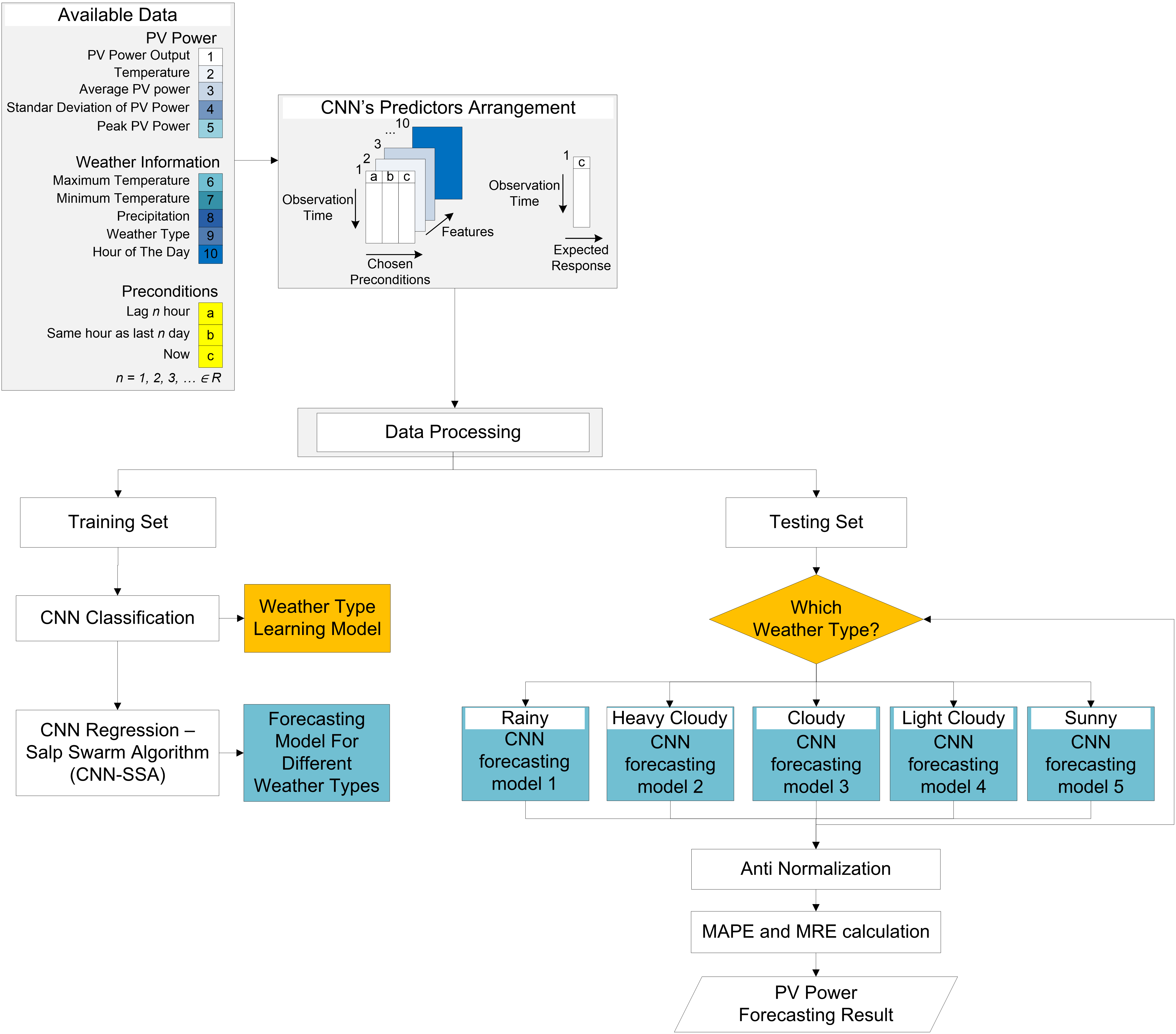
In this study’s short-term PV power forecasting, historical data were used as input variables. The data consisted of daily and hourly datasets. The hourly dataset consisted of historical PV power output and temperature. The daily dataset consisted of average PV power, standard deviation of PV power, peak PV power, maximum temperature, minimum temperature, precipitation, and weather type. In addition, the hour of the day was also accounted for as an input variable. Per the sunlight duration, the period of observation was set to 12 h per day, from 6 a.m. to 5 p.m. The arrangement of input variables is described in Figure 1. The ten potential input variables were indexed from 1 to 10 for PV power output, temperature, average PV power, standard deviation of PV power, peak PV power, maximum temperature, minimum temperature, precipitation, weather type, and hour of the day, respectively. The potential preconditions were indexed with the letters a to h for 1 h lag, 2 h lag, 3 h lag, same hour as last day, same hour as last 2 days, same hour as last 3 days, same hour as last 4 days, and present (recent), respectively. The available data with correlation coefficients used in Zhong et al. [44] were then tested to establish whether input variables were closely correlated with the PV power generation. Based on the t-test result, the input vectors with p-values lower than 0.05 were classified as significant and were used as input variables. The correlation coefficient results are listed in Table 1.
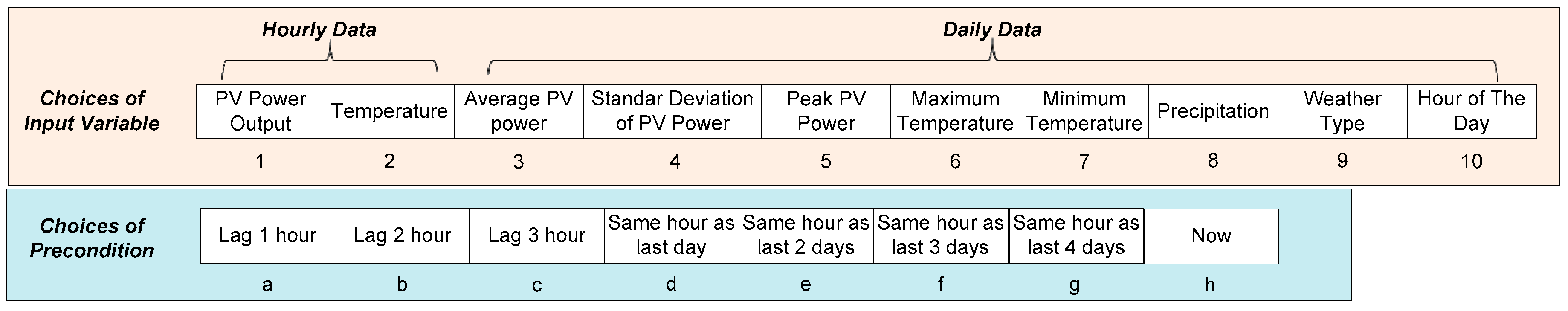
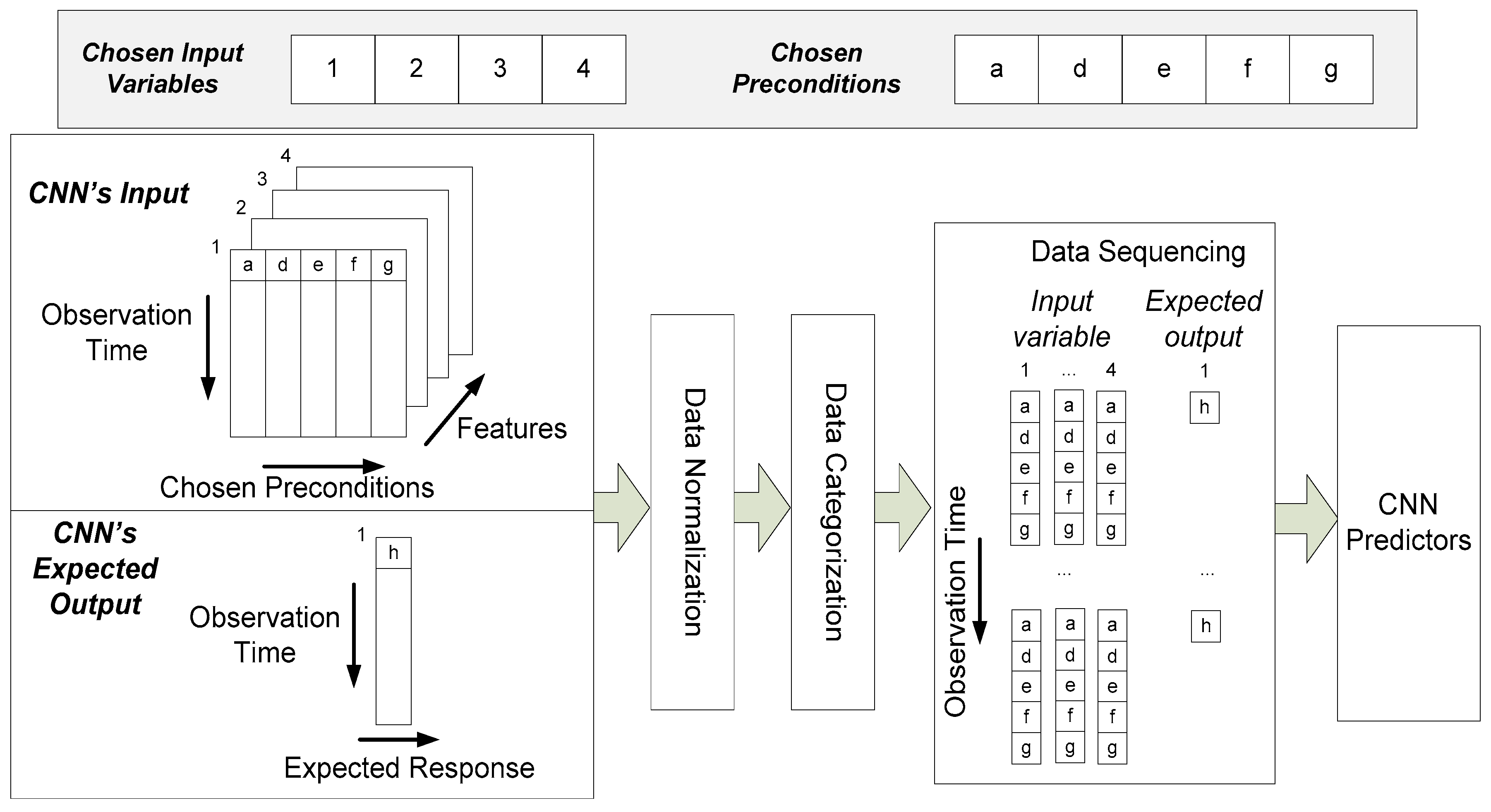
From the available input variables and preconditions that exhibited a close correlation with the PV power output, the model with the fewest input variables was constructed to generalize the practicability of the model. The computations between the input variables and preconditions were as follows. As an example, we take PV power output, temperature, average PV power, and the standard deviation of PV power as the chosen input variables—labeled as 1, 2, 3, and 4, respectively—as features of CNN predictors. Subsequently, 1 h lag, same hour as last day, same hour as last 2 days, same hour as last 3 days, and same hour as last 4 days are selected as the preconditions and labeled as a, d, e, f, and g, respectively. The CNN forecasting model requires a set of predictors and expected outputs.
The CNN predictor arrangement is described in Figure 2. For the CNN’s input, where we must apply the set of chosen preconditions for each feature, which is portrayed as a 3-D matrix such that the observations, the number of chosen preconditions, and the number of features represent the row, column, and width sizes, respectively. The CNN’s expected output constitutes a 2-D matrix for which the number of observations and responses (expected PV power outputs) represent its row and column sizes, respectively. Each of the predictors and the expected output pairs are then normalized, categorized, and sequenced. The data are normalized with max–min normalization. Subsequently, the expected output is categorized according to the historical weather type. To some extent, data categorization can be used to recognize crucial times during the observations, such as the peak time or huge decreases in the load demand. Last, the predictor–expected output pairs are rearranged based on their sequence per the observation times. The predictor matrix is transformed into a 4-D matrix such that the sizes of the predictors are given by the number of observations, the number of features, the number of responses, and the number of observations for the row, column, layer, and sequence, respectively. The arrangement of the expected output is also the same, but the sizes of the rows and columns are all set to 1 per the size of the response.
3. Proposed Forecasting Strategy
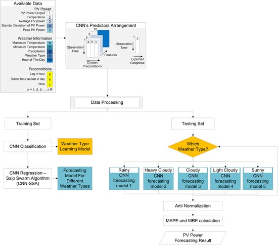
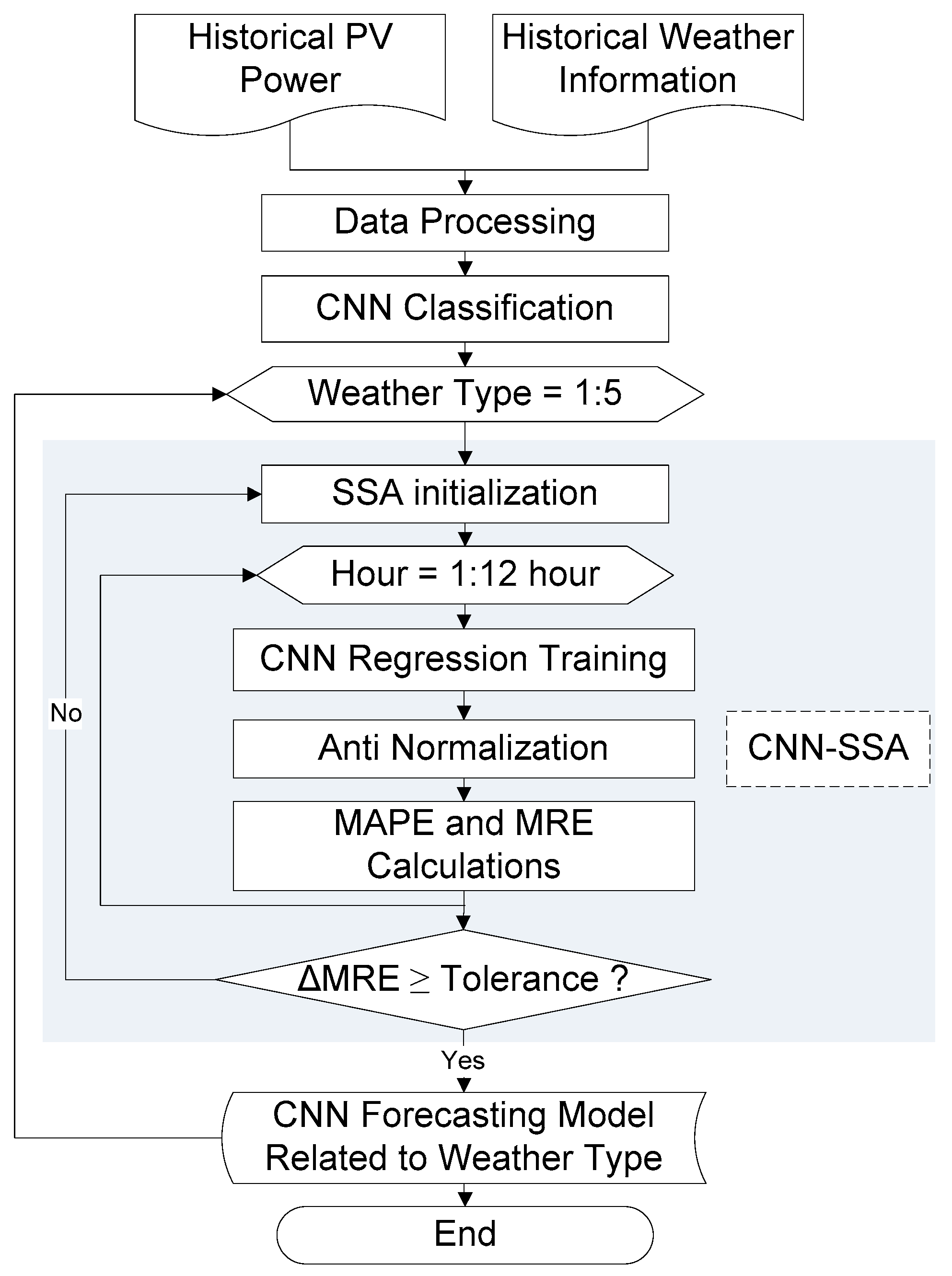
The proposed forecasting strategy consists of a CNN classification and an SSA-based CNN regression. The CNN classification is used to determine the weather type for the following day. The SSA is used to tune the CNN regression parameters. The CNN regression is used as the short-term forecasting model for PV power and the predictors, using the optimal parameter obtained from SSA. In the training stage, as depicted in Figure 3, the historical PV power and weather information is processed using the steps described in Section 2, with a set of CNN predictors closely correlated to the training PV power output expected. A set of CNN predictors and training outputs are subjected to CNN classification to label each of the training data sets with suitable weather types. In addition to the label, the structure of this CNN classification is recorded for use in the testing stage. The labeled training data set is then classified into the five weather types of rain, heavy cloudy, cloudy, light cloudy, and sunny. To obtain a close correlation and less variation in the data set, the grouped dataset is classified into observation hours. Subsequently, the SSA initializes the parameters of the CNN regression and the forecasting model is trained using SSA initial parameters. The forecasting result is anti-normalized and evaluated using the mean absolute percentage error (MAPE) and the mean relative error (MRE). The SSA identifies the best CNN parameters using the MRE as the objective function. If the MRE mismatch between the iterations is within the tolerance threshold, the SSA iteration is terminated and the best parameter of the CNN for the respective weather type and hour is recorded. For the rest of the weather-type model, the same process is applied for each hour of observation.
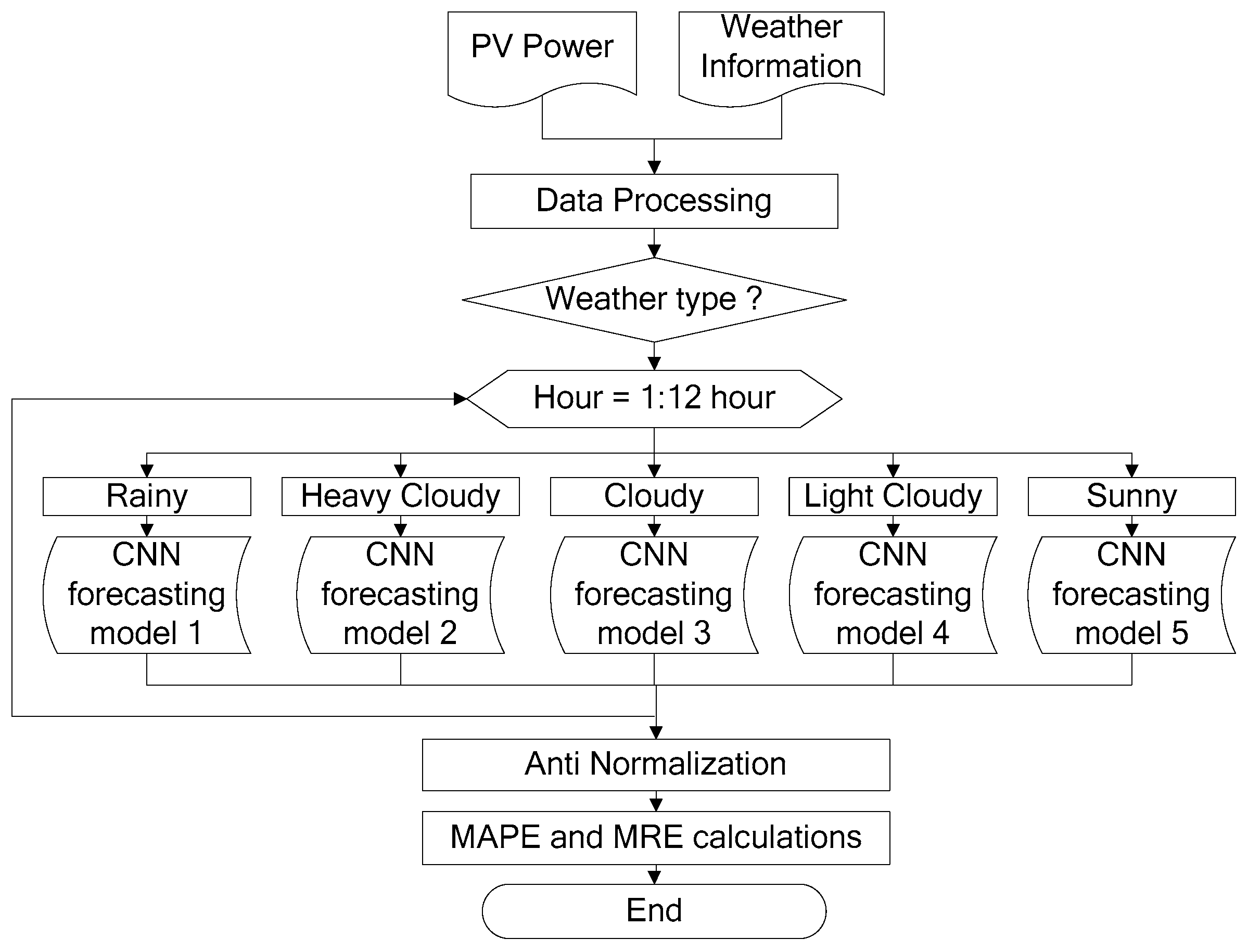
For the testing stage, as depicted in Figure 4, the recent PV power and weather information are used. The resulting data set is processed and subjected to the CNN classification to establish the weather type that is applicable for the day in question. The input variables are then fed into the respective CNN regression model based on the weather type. After the anti-normalization process, the forecasting model result is evaluated using the MAPE and the MRE. The following section is thereby divided into three sections for CNN classification, SSA-CNN regression, and benchmark algorithms.
3.1. CNN Classification For Suitable Weather-Type Identification
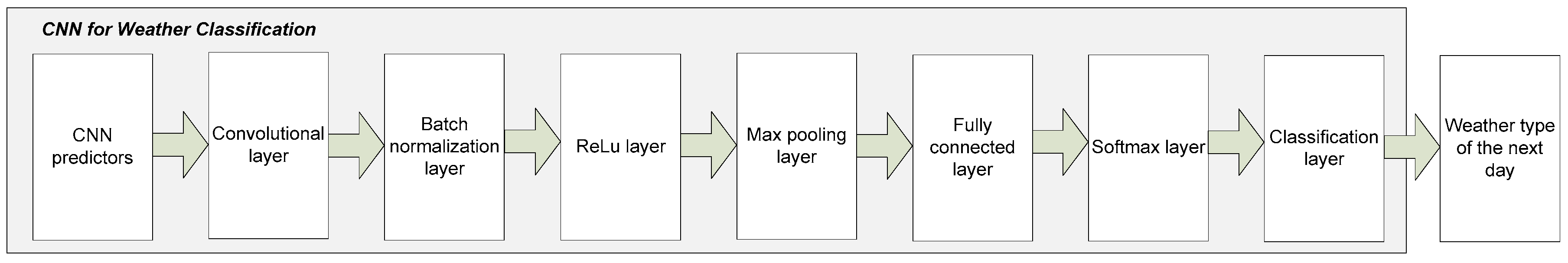
The CNN classification is constructed for investigating weather conditions before the forecasting approach is used. The CNN is constructed with multiple layers, such as the convolutional layer, max-pooling layer, rectified linear unit (ReLU) layer, batch normalization layer, softmax layer, and fully connected layer, as depicted in Figure 5. The batch normalization layer is inserted between the convolutional layer and the ReLU layer to accelerate the training of the CNNs and to reduce the sensitivity to the network initialization. The ReLU layer features a threshold operation for each element of the input, where any value less than zero is set to zero. The max-pooling layer is the layer that spatially rearranges the convolutional layer and extracts the feature map. In the pooling process, the number of parameters is reduced. The softmax layer produces a discrete probability distribution function over a multiclass classification.
According to the following CNN classification structure, the neurons in the convolutional layers must connect to the subregions of the layers (such as the max-pooling layer, batch normalization layer, and ReLU layer) instead of being fully connected as in other types of neural networks [45]. The neurons in the convolutional layer are spatially arranged in accordance with the model-correlated outcomes from the subregions [46] to reflect weight sharing among neurons, unlike in other types of neural networks, which include no weight sharing among the connections but instead produce the outcomes directly. In this research, the fully connected layer has five neurons corresponding to the five weather types.
3.2. SSA-CNN Regression For Short-Term PV Power Forecasting
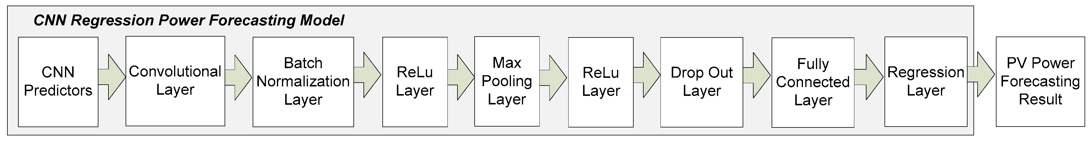
The CNN regression [30] is used as the forecasting model for the PV power output. The structure of the CNN regression, shown in Figure 6, consists of the convolutional layer, batch normalization layer, ReLU layer, max-pooling layer, drop-out layer, and fully connected layer, which is called the regression layer. The dropout layer is inserted between the ReLU layer and the fully connected layer to avoid overfitting, which may produce inaccurate forecasting results. The fully connected layer only has one neuron because the forecasted response is only the PV power output. In the CNN regression, the size of each layer must be initialized to obtain high-performance forecasting results. Due to the small dimension of the input layer, the convolutional layer and the max-pooling layer are set to having kernel size of two, corresponding to the two pixels in the input layout. In this research, SSA is integrated to obtain the best CNN regression initialization, particularly the size of the drop-out layer, the initial learning rate, and the mini-batch size.
The SSA [33] is developed using the behavior of salps in a chain formation regarding their hunting tactics. For optimization, these chains exert a significant effect on the SSA’s balancing of the exploration and exploitation inclinations by assisting it in escaping from local optima and preventing the problem of stagnation. In SSA, the population is formed using the chains of salps, of which two types exist: leaders and followers. When the agent is the front-runner, it is classified as the leader, whereas other salps are classified as followers. The role of the leader salp is to guide and direct the population’s next steps, and the follower salps pay attention to other peers.
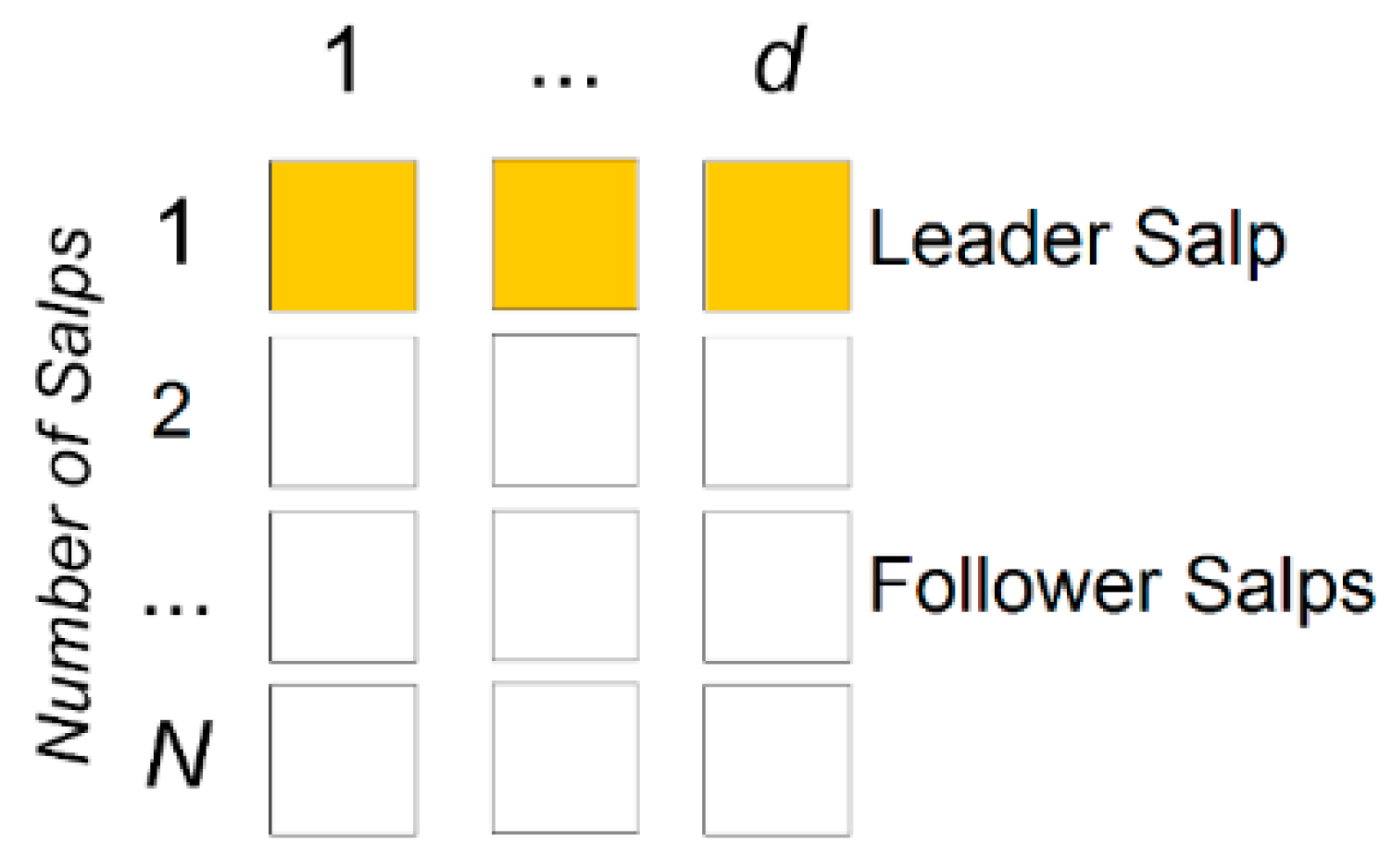
As shown in Figure 7, the salps’ positions during the exploration and exploitation phases are defined as an n-dimensional space, where n is the total number of variables. For a set of salps X consisting of N salps with d dimensions, an SSA population is recorded in an (N × d)-dimensional matrix. The salp population is then divided into two groups for leaders and followers. The leader is the salp at the front of the chain, and the rest of the salps are considered followers.
The salp chains are computed by updating the positions of the leader and follower salps. The updating process of the leader salp position is related to the food source. In the th dimension of the search space, the leader position is updated according to the food source position , which lies within the upper and lower bounds of and , respectively. The leader position is also updated based on the coefficients , , and , as in Equation (1):
where the coefficients and are uniform random numbers between [0,1]. For in particular, this coefficient represents the balance portion of exploration and exploitation, which is defined as follows:
where is the current iteration and is the maximum number of iterations. The incorporation of , , and demonstrates that the next position in the th dimension should move toward positive infinity or negative infinity, as well as the step size.
The updating process of the follower salps’ positions can then be modeled as follows:
where is the number of follower salps, is the iteration, and is the initial speed. , where , is a ratio of the final speed to the initial speed. Accordingly, the follower salps’ positions are obtained as follows:
where is the position of the th follower salp in the th dimension. In this study, SSA was used to identify optimal parameters for the proposed method and benchmark algorithms.
3.3. Benchmark Algorithms and Evaluation Index
To validate the performance of the proposed method, SVMs and an LSTM were used as benchmarks. These methods have been applied as forecasting models and have shown accurate results. The algorithms are summarized as follows.
3.3.1. Long Short-Term Memory-SSA (LSTM-SSA)
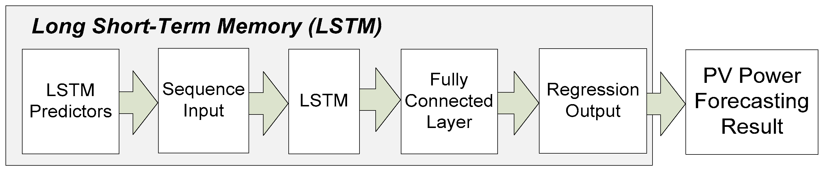
An LSTM [46] is a type of recurrent neural network that can collect information and determine whether to accumulate new information or to forget the information once a gate is triggered. The interaction between these gates enables an LSTM to model long-term dependencies and prevents gradient vanishing in the solution of time-series predictions. The LSTM structure is depicted in Figure 8. The sequence input is essentially the sequence arrangement of LSTM predictors that was shown in Section 2. In an LSTM, the size of the predictors is a two-dimensional time series in which the sizes of the predictors should be three-dimensional matrices for CNNs. As an SSA is integrated to an LSTM, seven parameters are searched by the SSA: (1) the number of hidden units, (2) max epoch, (3) gradient threshold, (4) initial learning rate, (5) learning rate decrease period, (6) learning rate decrease factor, and (7) mini-batch size.
3.3.2. Support Vector Machine-SSA (SVM-SSA)
An SVM [47,48] is a nonparametric technique using sequential minimal optimization to solve a decomposed equation for the input variables. For each iteration, a working set of two points is used to find a function f(x) that deviates from yt by a value not greater than the error in each previous training point for x. The result of the iteration process can be recalled as the mapping of the training data x into a high-dimensional feature space to represent the nonlinear relationships between the input variables and the targeted output. In an SVM, the weight of the α value is solved using an SSA.
3.3.3. Evaluation Index
The MAPE and MRE are used to evaluate the forecasting results relative to the actual PV power output at the observed hour t. The calculation of MAPE and MRE are as follows:
where is the number of observation hours, and
is the PV power plant capacity.
4. Simulation Results
The proposed method was simulated in a MATLAB 2018 environment running using an Intel Core i-73770 CPU operating at 3.40 GHz with 8 GB RAM. The SSA used 15 agents with a maximum of 100 iterations. For each tuning model, the best performance and error distribution were observed in ten trials. The SVM was set using the sequential minimal optimization solver using five kernels.
4.1. Test System
The test system had a capacity of 500 kWp and was located in the south of Taiwan. The site was located at a latitude of 22.71°N, a longitude of 120.54°E, and an altitude of 43 m. The historical hourly data was collected from January to December of 2017. The test system consisted of historical data for the PV power output, average temperature, relative humidity, clear-sky radiation, wind speed, and day stamp. These historical data were grouped in terms of the CNN classifications for five weather types: rain, heavy cloudy, cloudy, light cloudy, and sunny. The forecasting model required five preconditions, which were same hour as the last 1, 2, 3, and 4 days; lagged 2 h; and the hour stamp. For the cloudy weather model, seven preconditions were used, which were same hour as the last 1, 2, 3, and 4 days; lagged 2 and 3 h; and hour stamp. The arrangement of the CNN predictors was per the explanation given in Section 2. The datasets for each weather type included 14, 23, 36, 60, and 42 days for rain, heavy cloudy, cloudy, light cloudy, and sunny, respectively. The training and testing datasets were set to 70% and 30%, respectively, of the total dataset length. With the approach of a real-time situation, in which the longer historical PV power and weather information may be unavailable, only the four previous days’ historical data were incorporated as the CNN predictors for forecasting the next day.
4.2. Short-Term PV Power Forecasting
The optimal CNN, LSTM, and SVM parameters searched for using the SSA for each weather type are shown in Table 2 and Table 3, and Figure 9, respectively. For the CNN-SSA method, five parameters were tuned, as shown in Table 2. The kernel size of the convolutional layer and the max-pooling layer ranged between 2 and 3 because the width of the input layer was only 5 × 5. The dropout layer value ranged between 0.315 and 0.5, the initial learning rate between 0.012 and 0.01875, and the mini-batch size ranged between 2 and 4.
For the LSTM-SSA method, seven parameters were tuned: hidden units, max epoch, gradient threshold, initial learn rate, learning rate decrease period, and learning rate decrease factor, as shown in Table 3. The number of hidden units in rainy, cloudy, and sunny were 7, and those in heavy cloudy and light cloudy were 8 and 3, respectively. The max epoch value varied between 178 and 200 epochs. The gradient threshold ranged from 479 to 546, initial learn rate from 0.010172 to 0.028262, learning rate decrease period from 55 to 96, and the learning rate decrease factor from 0.505356 to 0.819285.
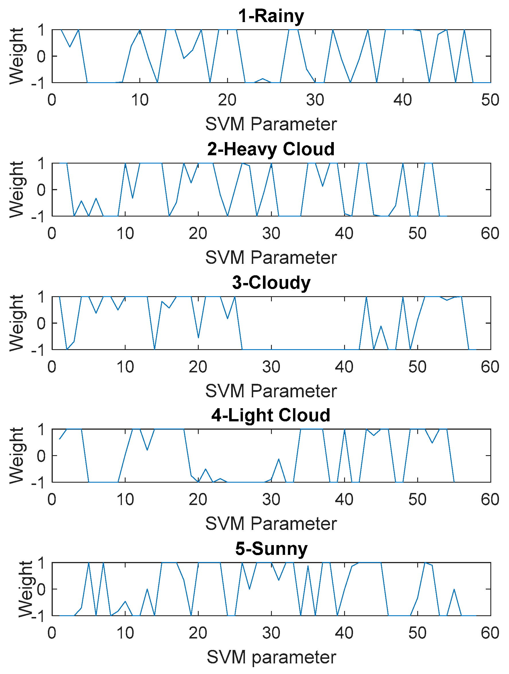
A set of parameters represents the SVM-SSA weight. The SVM kernel was set to 5. The values of were 50, 54, 58, 55, and 58 for rain, heavy cloudy, cloudy, light cloudy, and sunny, respectively. The weights were bounded between [−1, 1]. The tuned SVM-SSA parameters are shown in Figure 9.
The results of the proposed CNN-SSA PV power forecasting in the training stage are seen in Table 4, including one-day-ahead and three-day-ahead forecasts for the five weather types. To obtain a broader view of the forecasting performance, the observation time was extended to three days ahead, which exhibited variations due to the nonstationary nature of PV power generation. In the day-ahead forecasting results, the sunny model achieved the lowest MRE value of 1.43% and MAPE value of 5.34%. The light cloudy model achieved the highest MRE value of 3.8%; the rain model achieved the highest MAPE value of 42.55%. To obtain the optimal forecasting model, the computation times ranged between 14.57 and 16.76 min, which are plausible values for the training stage. In the three-days-ahead observation, the lowest MRE value of 2.33% and MAPE value of 15.30% were achieved for sunny and light cloudy models, respectively. The heavy cloudy model achieved the worst MRE value of 4.41% and MAPE value of 59.61%. The computation cost for the three-days-ahead model varied from 13.62 to 15.93 min.
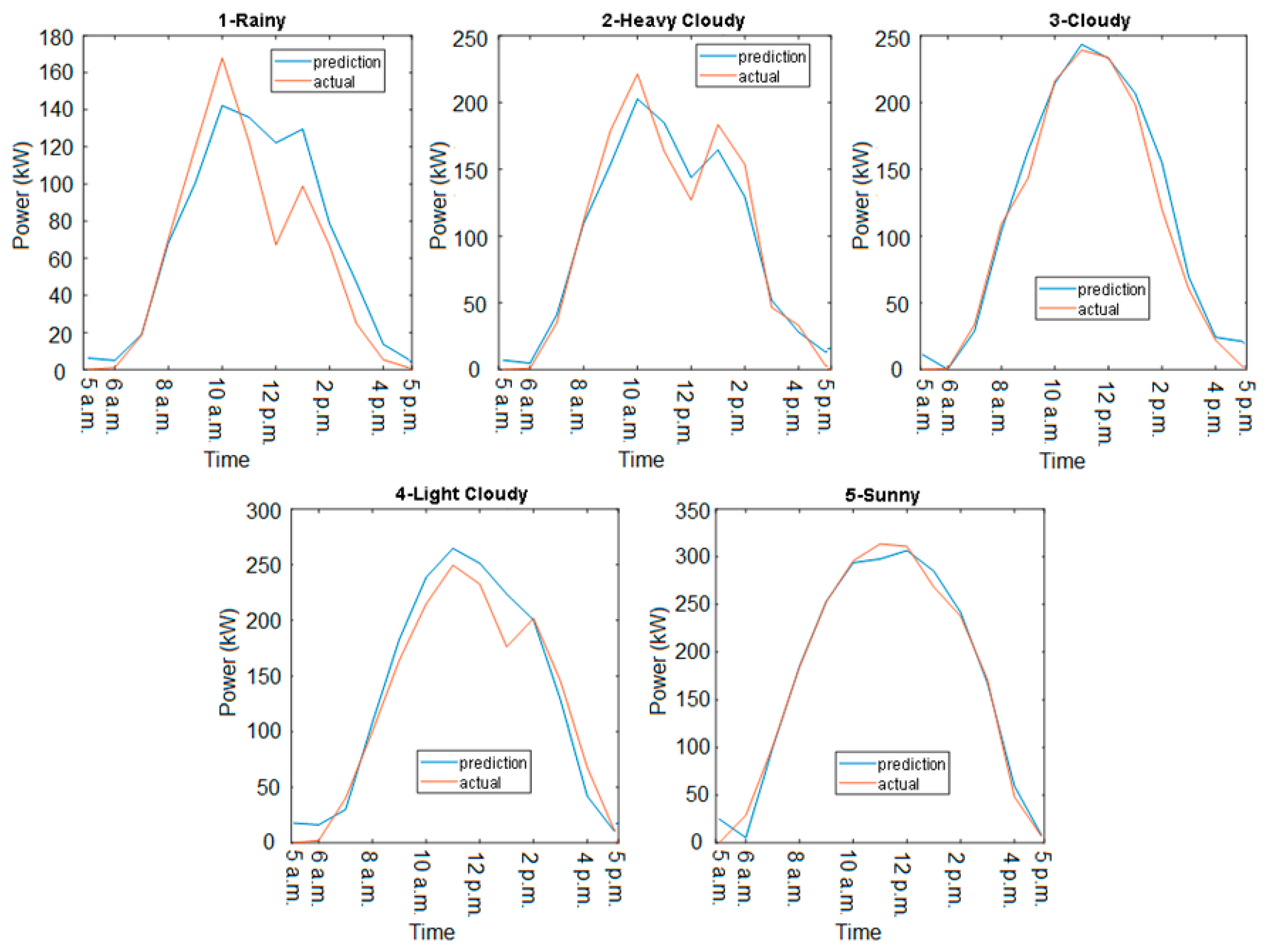
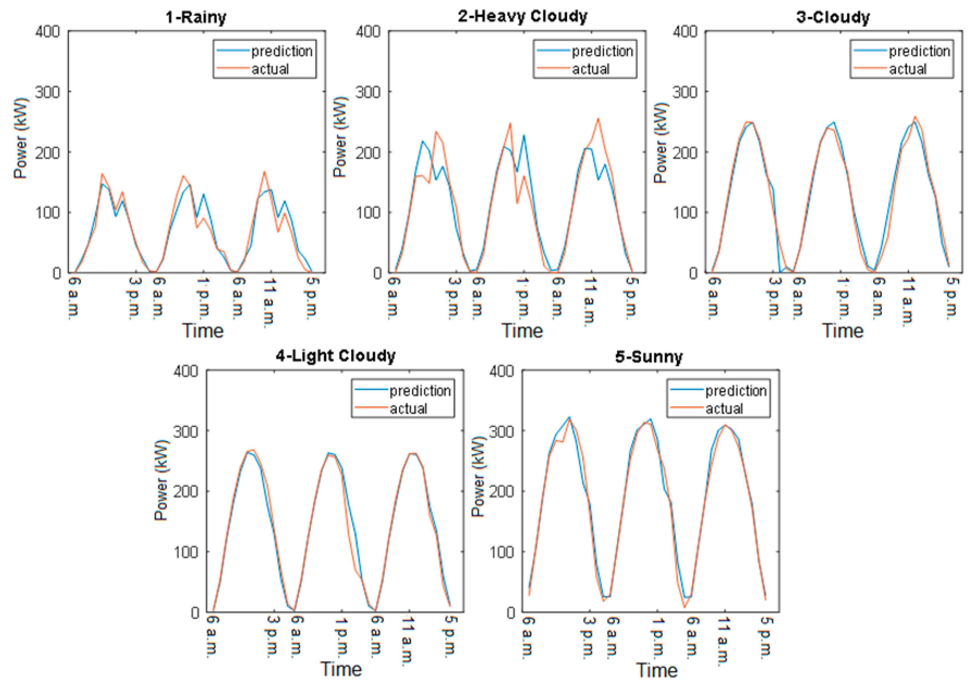
The day-ahead and three-days-ahead forecasting results are depicted in Figure 10 and Figure 11, respectively. In Figure 10, the y-axis represents the PV power in kW and the x-axis represents the hours of observation within a day. Each day, the PV power was observed between 6 a.m. and 5 p.m. because this was the time during which the PV power plant generated power. If the forecasting horizon was extended to three days, the observation hour was extended from 12 to 36 h. By contrast, the x-axis represents the hours of observation within three days, including 3 days × 12 observation hours between 6 a.m. and 5 p.m.; thus, the x-axis comprises 36 points in Figure 11. Using the proposed CNN-SSA method, the actual PV power pattern is represented, particularly for sunny and cloud models in the day-ahead observation, in Figure 10, and for the cloudy, heavy cloudy, and sunny models in three-days-ahead observation in Figure 11. In the rainy and heavy cloudy models, the gap between the actual PV power and the predictions was perceptible, particularly after the first peak of the PV power generation was reached, due to nonstationary variation at this time; this was more visible in three-days-ahead observation.
Table 5 details the evaluation of the proposed CNN-SSA in comparison to benchmark algorithms for three-days-ahead observations. Overall, the CNN-SSA method yielded the lowest MRE and MAPE values among the benchmark algorithms. The rainy model achieved an MRE of 2.62%, whereas the LSTM-SSA and SVM-SSA achieved MREs of 3.7% and 4.69%, respectively. The MAPE of the proposed method was 21.17%, whereas the LSTM-SSA and SVM-SSA achieved MAPE values of 32.1% and 34.75%, respectively. For the heavy-cloud model, the proposed method had an MRE value of 3.14% and an MAPE value of 15.27%, whereas the LSTM-SSA and SVM-SSA achieved MREs of only 6.39% and 5.63% and MAPE values of 28.83% and 21.56%, respectively. By contrast, the SVM-SSA in the cloud model achieved an MRE value of 2.62% and an MAPE value of 16.25%, outperforming the LSTM-SSA, for which the MRE value was 4.34% and the MAPE value was 21.56%. However, the SVM-SSA performance was inferior to the CNN-SSA performance, which achieved an MRE of 2.55% and an MAPE of 12.25%. In the light cloudy model, the proposed method outperformed the LSTM-SSA and SVM-SSA methods with an MRE value of 2.11% and an MAPE value of 12.75%. In the sunny model, the CNN-SSA method achieved an MRE of 2.45% and an MAPE of 5.5%; the LSTM-SSA method performed worse with an MRE of 4.11% and MAPE of 9.6%. The SVM-SSA method achieved an MRE value of 2.76% and an MAPE value of 7.93%.
By comparison with the general method, the integration of an SSA significantly improved the forecasting accuracy of the traditional CNN, LSTM, and SVM. Except for the rainy model, the traditional SVM showed better accuracy than the SVM-SSA. However, for the rest of the weather models, forecasting accuracy of the SVM-SSA surpassed the traditional SVM by 3.65%, 8.47%, 2.38%, and 2.94% MAPE difference for the heavy cloudy, cloudy, light cloudy, and sunny models, respectively. In the traditional LSTM, there were 3.75%, 4.53%, 5.38%, 8.32%, and 6.91% MAPE differences for each of the rainy, heavy cloudy, cloudy, light cloudy, and sunny models, respectively. Meanwhile in the traditional CNN case, the SSA integration resulted in the forecasting accuracy improvement of 8.55%, 38.60%, 8.37%, 0.04%, and 7.41% for the rainy, heavy cloudy, cloudy, light cloudy, and sunny models, respectively. If we observed the trend in the MRE, the forecasting accuracies increased by 0.32%, 0.88%, 0.19%, 0.59%, and 0.08% for each weather model for CNN-SSA and the traditional CNN comparison. For the LSTM-SSA relative to the traditional LSTM, the MRE also decreased by 2.29%, 0.12%, 0.66%, 0.74%, and 1.85% for each of the rainy, heavy cloudy, cloudy, light cloudy, and sunny models, respectively. For the traditional LSTM relative to the LSTM-SSA, the improvement trends shown in the heavy cloudy, cloudy, light cloudy, and sunny models were 3.65%, 8.47%, 2.38%, and 2.94%, respectively; in contrast, the rainy model showed an increase in MRE of 0.10%.
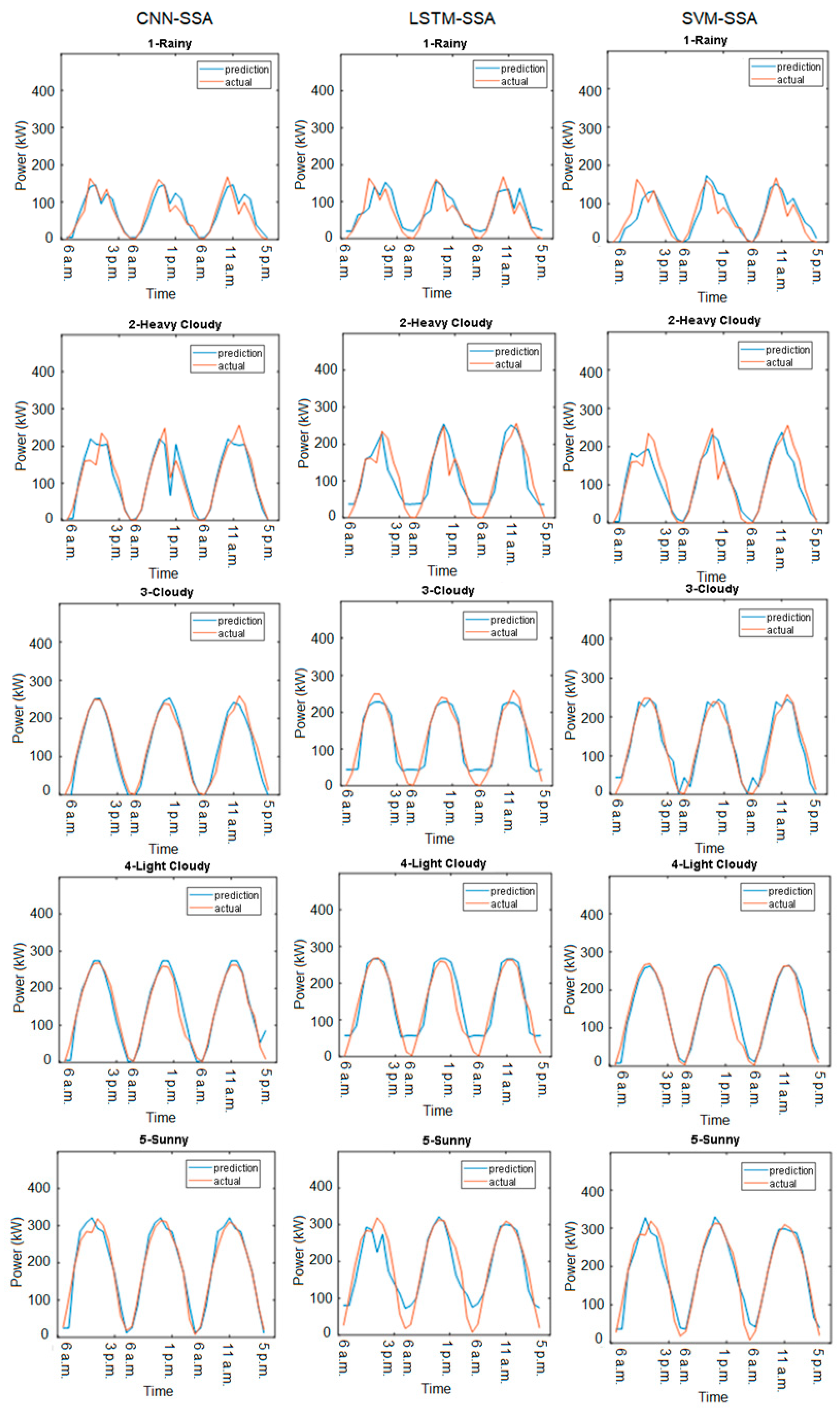
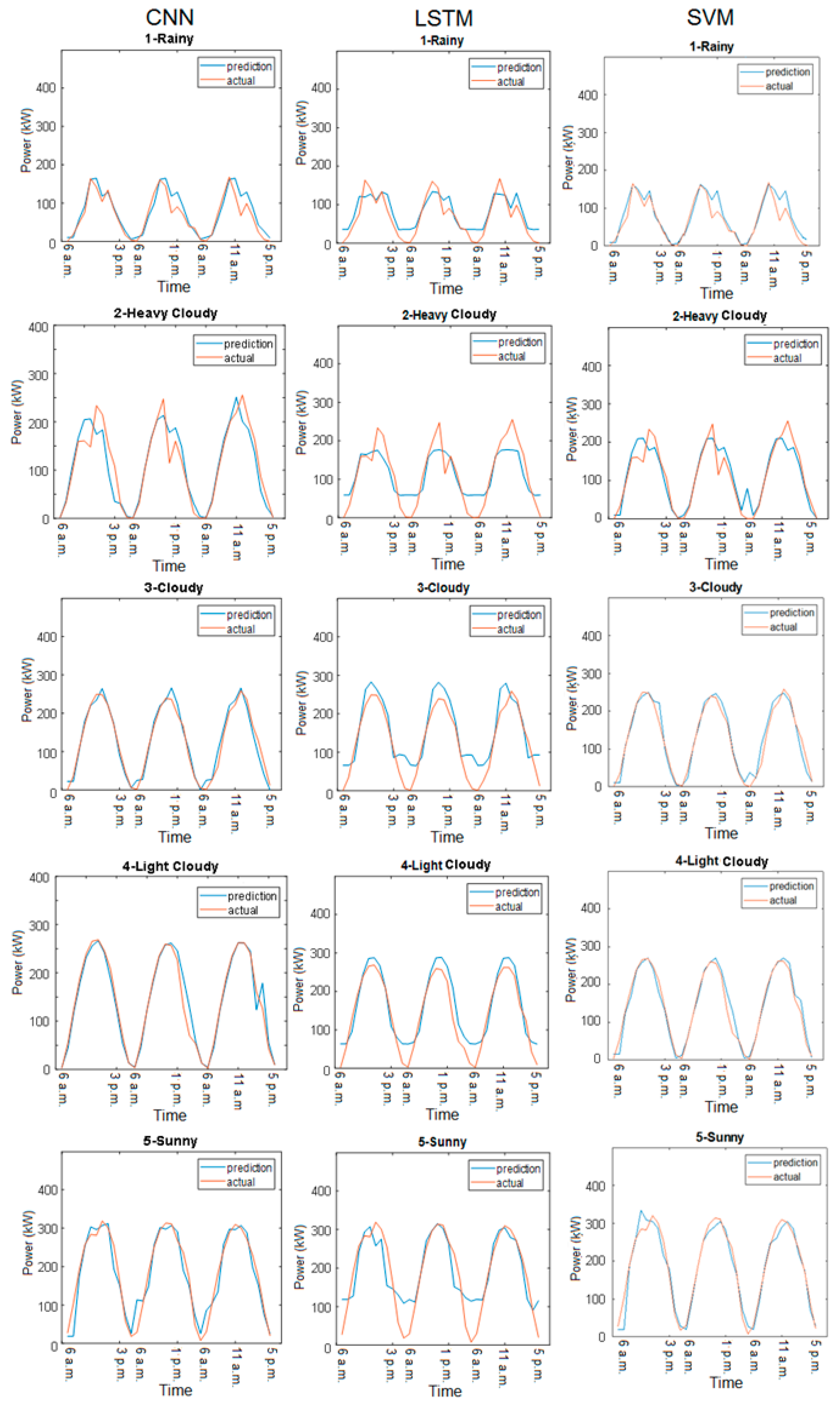
The plots for the three-days-ahead forecasting results are shown in Figure 12. In the rain and heavy cloud models, the CNN-SSA method provided an accurate representation of the actual PV power, especially at peak times. In the cloudy and light cloudy models, the actual PV power exhibited one peak. The CNN-SSA and LSTM-SSA methods represented the pattern, whereas SVM-SSA was likely to predict two peaks. The CNN-SSA performance was better than the LSTM-SSA performance from the beginning of the forecast period until the last of the forecasting hours. In the sunny model, the CNN-SSA and SVM-SSA methods represented the actual PV power pattern better than the LSTM-SSA did. The LSTM-SSA method performed poorly at the beginning and end of the observation time, during which the CNN-SSA method outperformed the benchmark algorithms. In comparison with the traditional benchmark algorithms as seen in Figure 13, the proposed method performed well. As can be seen, the traditional LSTM could not follow the actual load pattern in the beginning and peak observation hours. This happened due to the general input variables applied to the LSTM for each hour, which made the LSTM more prone to sudden changes in the PV power output. Different to the LSTM, the CNN and SVM had a more generalized ability to overcome sudden change for each observation hour.
4.3. Discussions
The proposed CNN-SSA method was designed to provide an accurate short-term PV power forecasting model that can overcome the drawbacks of large sets of historical data [16] and intensive spatial [29] and geographical information [32]. To examine the performance of the proposed method, the proposed CNN-SSA method was observed for a day ahead and extended to three days ahead to establish whether nonstationary variation affected the accuracy of the proposed method. For both day-ahead and three-days-ahead forecasting, the proposed CNN-SSA method outperformed the benchmark algorithms, which were evaluated as having MAPE values of 1.43% and 5.05% in the training and testing stages, respectively, for the sunny model. The performance of the rainy and heavy cloudy models was expected to be inferior to the rest of the models because of their greater PV power variation. Nevertheless, the proposed method maintained an MAPE value of 21.17% and an MRE value of 2.62%, which were superior to the benchmark algorithms’ corresponding values. Moreover, the proposed method flexibly identified the optimal forecasting model because the SSA was integrated into the CNN structure, which resolved the inefficiency of the CNN parameter trial and error [23,24]. The historical data arrangement in the proposed method enabled the time series data set to be rearranged as CNN predictors, which accommodated multiple input variables associated with the expected forecasting outcomes without the need for bounding within specific image formats [22]. Despite the accuracy of the proposed CNN-SSA method, it required more time to produce an accurate model, ranging between 12 and 28 min, whereas the benchmark algorithms required a quarter of the proposed method’s computation time.
As seen in Figure 12, though, the performance of CNN-SSA in cloudy, light cloudy, and sunny models fitted the actual PV power pattern closely, while the forecasting model struggled to follow the peak time in the sunny model. For the rainy and heavy cloudy models, the proposed method could not maintain a gap as close as in the sunny model. This condition implied that the uncertainty of the PV power output in the rainy and heavy cloudy models, and peak time of sunny model, to be addressed further. This condition also happened because the forecasting model was built from less training data, which suppressed the ability of the CNN to learn the uncertainty of the PV power. Nevertheless, the proposed CNN-SSA provided an accurate forecasting algorithm of the PV power that could accommodate multiple inputs and responses at once in comparison to the benchmark algorithm.
For a comparison of the proposed method with other CNN applications in PV power forecasting, the forecasting strategy in Jeong and Kim [49] accommodated the temporal PV power generation at multiple-site PV power plants. The CNN in Jeong and Kim [49] took a space-time matrix as the input, which consisted of the historical PV power generation of the preferred observation time collected from multiple PV sites. The CNN was applied to two-hours-ahead and six-hours-ahead predictions. In the proposed method, the proposed CNN-SSA method adopts multiple input variables, including the related historical (for training) and forecast (for prediction) weather data for applications of longer forecasting horizon of one-day-ahead and up to three-day-ahead PV power forecasting.
In addition, as a longer forecasting horizon is needed, a larger CNN structure should be employed with many more parameters to be tuned. Since there is no general rule to determine the best parameters of a CNN, the smallest number of CNN parameters was chosen for the input size in Jeong and Kim [49], which was much smaller than the number used in AlexNet [50] and VGGNet [51]. In the proposed method, the SSA was used to overcome this issue instead of intuitively choosing the suitable parameters. Therefore, the more suitable parameters in the proposed CNN predictors could be achieved for a larger structure.
In Jeong and Kim [49], a greedy adjoining algorithm (GAA) was used to indirectly capture cloud cover and movements conducted for the geographic location and historical dataset of multi-site PV generation, an approach that is suitable for a very short forecasting horizon. The proposed method uses the weather classification approach to improve the forecasting accuracy under the PV power generation uncertainty due to daily weather variations. The proposed method is thus more appropriate for a longer forecasting horizon from one to three days ahead.
5. Conclusions
This paper proposes a short-term PV power forecasting algorithm based on a CNN-SSA. CNN regression is used to construct the prediction model, and SSA is used to identify the optimal CNN parameter. CNN classification is used for the CNN-SSA to obtain the correct weather type. The results show the proposed method provided better accuracy than the benchmark algorithms did. The proposed algorithm provides a simple approach for the creation of this forecasting method, yet guarantees consistent accuracy within the day-ahead to the three-days-ahead forecasting windows. Although only five CNN regression models were used to establish the forecasting models, the proposed method can be extended to other models for more accurate predictions. Addressing the uncertainty, especially for rainy weather, heavy cloudy weather, and the peak time, is the future work of this study. Furthermore, forecasting on typhoon days represents a potential challenge for future research.
Author Contributions
This paper is a collaborative work of all authors. Conceptualization, H.A.; methodology, H.A., H.-T.Y., and C.-M.H.; software, H.A.; validation, H.A.; writing—original draft preparation, H.A.; supervision, H.-T.Y. and C.-M.H.; funding acquisition, H.A., H.-T.Y., and C.-M.H. All authors have read and agreed to the published version of the manuscript.
Funding
This work was supported by the Ministry of Science and Technology, Taiwan, under the grants MOST 109-3116-F-006-017-CC2 and 108-3116-F-168-001-CC2. The work of H.A. was supported by the Indonesia Endowment Fund for Education (LPDP).
Conflicts of Interest
The authors declare no conflict of interest.
References
- Alkaabi, S.; Zeineldin, H.; Khadkikar, V. Short-Term Reactive Power Planning to Minimize Cost of Energy Losses Considering PV Systems. IEEE Trans. Smart Grid 2019, 10, 2923–2935. [Google Scholar] [CrossRef]
- Fleischhacker, A.; Auer, H.; Lettner, G.; Botterud, A. Sharing Solar PV and Energy Storage in Apartment Buildings: Resource Allocation and Pricing. IEEE Trans. Smart Grid 2019, 10, 3963–3973. [Google Scholar] [CrossRef]
- Chakraborty, P.; Baeyens, E.; Khargonekar, P.; Poolla, K.; Varaiya, P. Analysis of Solar Energy Aggregation Under Various Billing Mechanisms. IEEE Trans. Smart Grid 2019, 10, 4175–4187. [Google Scholar] [CrossRef] [Green Version]
- Gao, S.; Jia, H.; Marnay, C. Techno-Economic Evaluation of Mixed AC and DC Power Distribution Network for Integrating Large-Scale Photovoltaic Power Generation. IEEE Access 2019, 7, 105019–105029. [Google Scholar] [CrossRef]
- Mills, A.; Wiser, R. Implications of Wide-Area Geographic Diversity for Short-Term Variability of Solar Power; Technical Report LBNL-3884E; Lawrence Berkeley National Laboratory: Washington, DC, USA, 2010. [Google Scholar]
- Zhang, J.; Hodge, B.M.; Lu, S.; Hamann, H.F.; Lehman, B.; Simmons, J.; Campos, E.; Banunarayanan, V.; Black, J.; Tedesco, J. Baseline and target values for regional and point PV power forecasts: Toward improved solar forecasting. Sol. Energy 2015, 122, 804–819. [Google Scholar] [CrossRef] [Green Version]
- Yang, H.T.; Liao, J. MF-APSO-Based Multiobjective Optimization for PV System Reactive Power Regulation. IEEE Trans. Sustain. Energy 2015, 6, 1346–1355. [Google Scholar] [CrossRef]
- Di Piazza, M.; Luna, M.; La Tona, G.; Di Piazza, A. Improving Grid Integration of Hybrid PV-Storage Systems Through a Suitable Energy Management Strategy. IEEE Trans. Ind. Appl. 2019, 55, 60–68. [Google Scholar] [CrossRef]
- Nguyen, Q.; Padullaparti, H.; Lao, K.; Santoso, S.; Ke, X.; Samaan, N. Exact Optimal Power Dispatch in Unbalanced Distribution Systems with High PV Penetration. IEEE Trans. Power Syst. 2019, 34, 718–728. [Google Scholar] [CrossRef]
- De Giorgi, M.G.; Malvoni, M.; Congedo, P.M. Photovoltaic power forecasting using statistical methods: Impact of weather data. IET Sci. Meas. Technol. 2014, 8, 90–97. [Google Scholar] [CrossRef]
- Raza, M.Q.; Nadarajah, M.; Ekanayake, C. On recent advances in PV output power forecast. Sol. Energy 2016, 136, 125–144. [Google Scholar] [CrossRef]
- Sobri, S.; Koohi-Kamali, S.; Rahim, N.A. Solar photovoltaic generation forecasting methods: A review. Energy Convers. Manag. 2018, 156, 459–497. [Google Scholar] [CrossRef]
- Mellit, A.; Massi Pavan, A.; Lughi, V. Short-term forecasting of power production in a large-scale photovoltaic plant. Sol. Energy 2014, 105, 401–413. [Google Scholar] [CrossRef]
- Dolara, A.; Grimaccia, F.; Leva, S.; Mussetta, M.; Ogliari, E. A physical hybrid artificial neural network for short term forecasting of PV plant power output. Energies 2015, 8, 1138–1153. [Google Scholar] [CrossRef] [Green Version]
- Nespoli, A.; Ogliari, E.; Leva, S.; Pavan, A.M.; Mellit, A.; Lughi, V.; Dolara, A. Day-Ahead Photovoltaic Forecasting: A Comparison of the Most Effective Techniques. Energies 2019, 12, 1621. [Google Scholar] [CrossRef] [Green Version]
- Zeng, J.; Qiao, W. Short-term solar power prediction using a support vector machine. Renew. Energy 2013, 52, 118–127. [Google Scholar] [CrossRef]
- Preda, S.; Oprea, S.; Bâra, A.; Belciu (Velicanu), A. PV Forecasting Using Support Vector Machine Learning in a Big Data Analytics Context. Symmetry 2018, 10, 748. [Google Scholar] [CrossRef] [Green Version]
- Li, G.; Wang, H.; Zhang, S.; Xin, J.; Liu, H. Recurrent Neural Networks Based Photovoltaic Power Forecasting Approach. Energies 2019, 12, 2538. [Google Scholar] [CrossRef] [Green Version]
- Ju, Y.; Sun, G.; Chen, Q.; Zhang, M.; Zhu, H.; Rehman, M. A Model Combining Convolutional Neural Network and LightGBM Algorithm for Ultra-Short-Term Wind Power Forecasting. IEEE Access 2019, 7, 28309–28318. [Google Scholar] [CrossRef]
- Yan, K.; Li, W.; Ji, Z.; Qi, M.; Du, Y. A Hybrid LSTM Neural Network for Energy Consumption Forecasting of Individual Households. IEEE Access 2019, 7, 157633–157642. [Google Scholar] [CrossRef]
- Han, L.; Peng, Y.; Li, Y.; Yong, B.; Zhou, Q.; Shu, L. Enhanced Deep Networks for Short-Term and Medium-Term Load Forecasting. IEEE Access 2019, 7, 4045–4055. [Google Scholar] [CrossRef]
- Zhang, H.; Cheng, L.; Ding, T.; Cheung, K.W.; Liang, Z.; Wei, Z.; Sun, G. Hybrid method for short-term photovoltaic power forecasting based on deep convolutional neural network. IET Gener. Transm. Distrib. 2018, 12, 4557–4567. [Google Scholar] [CrossRef]
- Huang, C.; Kuo, P. Multiple-Input Deep Convolutional Neural Network Model for Short-Term Photovoltaic Power Forecasting. IEEE Access 2019, 7, 74822–74834. [Google Scholar] [CrossRef]
- Wan, R.; Mei, S.; Wang, J.; Liu, M.; Yang, F. Multivariate Temporal Convolutional Network: A Deep Neural Networks Approach for Multivariate Time Series Forecasting. Electronics 2019, 8, 876. [Google Scholar] [CrossRef] [Green Version]
- Deng, Z.; Wang, B.; Xu, Y.; Xu, T.; Liu, C.; Zhu, Z. Multi-Scale Convolutional Neural Network with Time-Cognition for Multi-Step Short-Term Load Forecasting. IEEE Access 2019, 7, 88058–88071. [Google Scholar] [CrossRef]
- Du, L.; Zhang, L.; Tian, X. Deep Power Forecasting Model for Building Attached Photovoltaic System. IEEE Access 2018, 6, 52639–52651. [Google Scholar] [CrossRef]
- Lee, W.; Kim, K.; Park, J.; Kim, J.; Kim, Y. Forecasting Solar Power Using Long-Short Term Memory and Convolutional Neural Networks. IEEE Access 2018, 6, 73068–73080. [Google Scholar] [CrossRef]
- Riaz, S.; Arshad, A.; Jiao, L. Fuzzy Rough C-Mean Based Unsupervised CNN Clustering for Large-Scale Image Data. Appl. Sci. 2018, 8, 1869. [Google Scholar] [CrossRef] [Green Version]
- Nam, S.; Hur, J. Probabilistic Forecasting Model of Solar Power Outputs Based on the Naïve Bayes Classifier and Kriging Models. Energies 2018, 11, 2982. [Google Scholar] [CrossRef] [Green Version]
- Suresh, V.; Janik, P.; Rezmer, J.; Leonowicz, Z. Forecasting Solar PV Output Using Convolutional Neural Networks with a Sliding Window Algorithm. Energies 2020, 13, 723. [Google Scholar] [CrossRef] [Green Version]
- Zhao, B.; Lu, H.; Chen, S.; Liu, J.; Wu, D. Convolutional neural networks for time series classification. J. Syst. Eng. Electron. 2017, 28, 162169. [Google Scholar] [CrossRef]
- Miyazaki, Y.; Kameda, Y.; Kondoh, J. A Power-Forecasting Method for Geographically Distributed PV Power Systems using Their Previous Datasets. Energies 2019, 12, 4815. [Google Scholar] [CrossRef] [Green Version]
- Mirjalili, S.; Gandomi, A.; Mirjalili, S.M.; Saremi, S.; Faris, H.; Mirjalili, S.M. Salp Swarm Algorithm: A bio-inspired optimizer for engineering design problems. Adv. Eng. Softw. 2017, 114, 163–191. [Google Scholar] [CrossRef]
- Saez, D.; Avila, F.; Olivares, D.; Canizares, C.; Marin, L. Fuzzy Prediction Interval Models for Forecasting Renewable Resources and Loads in Microgrids. IEEE Trans. Smart Grid 2015, 6, 548–556. [Google Scholar] [CrossRef] [Green Version]
- Hong, T.; Pinson, P.; Fan, S.; Zareipour, H.; Troccoli, A.; Hyndman, R. Probabilistic Energy Forecasting: Global Energy Forecasting Competition 2014 and Beyond. Int. J. Forecast. 2016, 32, 896–913. [Google Scholar] [CrossRef] [Green Version]
- Wang, H.; Yi, H.; Peng, J.; Wang, G.; Liu, Y.; Jiang, H.; Liu, W. Deterministic and Probabilistic Forecasting of Photovoltaic Power Based on Deep Convolutional Neural Network. Energy Convers. Manag. 2017, 153, 409–422. [Google Scholar] [CrossRef]
- Bracale, A.; Caramia, P.; Carpinelli, G.; Di Fazio, A.; Ferruzzi, G. A Bayesian Method for Short-Term Probabilistic Forecasting of Photovoltaic Generation in Smart Grid Operation and Control. Energies 2013, 6, 733–747. [Google Scholar] [CrossRef] [Green Version]
- Ruiz-Rodriguez, F.J.; Hernandez, J.C.; Jurado, F. Probabilistic load flow for photovoltaic distributed generation using the Cornish-Fisher expansion. Electr. Power Syst. Res. 2012, 89, 129–138. [Google Scholar] [CrossRef]
- Antonanzas, J.; Osorio, N.; Escobar, R.; Urraca, R.; Martinez-De-Pison, F.; Antonanzas-Torres, F. Review of photovoltaic power forecasting. Sol. Energy 2016, 136, 78–111. [Google Scholar] [CrossRef]
- Mellit, A.; Massi Pavan, A. A 24-h forecast of solar irradiance using artificial neural network: Application for performance prediction of a grid-connected {PV} plant at Trieste, Italy. Sol. Energy 2010, 84, 807–821. [Google Scholar] [CrossRef]
- Brecl, K.; Topič, M. Photovoltaics (PV) System Energy Forecast on the Basis of the Local Weather Forecast: Problems, Uncertainties and Solutions. Energies 2018, 11, 1143. [Google Scholar] [CrossRef] [Green Version]
- Kim, S.; Jung, J.; Sim, M. A Two-Step Approach to Solar Power Generation Prediction Based on Weather Data Using Machine Learning. Sustainability 2019, 11, 1501. [Google Scholar] [CrossRef] [Green Version]
- Alom, M.Z.; Taha, T.M.; Yakopcic, C.; Westberg, S.; Sidike, P.; Nasrin, M.S.; Hasan, M.; Van Essen, B.C.; Awwal, A.A.S.; Asari, V.K. A State-of-the-Art Survey on Deep Learning Theory and Architectures. Electronics 2019, 8, 292. [Google Scholar] [CrossRef] [Green Version]
- Zhong, J.; Liu, L.; Sun, Q.; Wang, X. Prediction of Photovoltaic Power Generation Based on General Regression and Back Propagation Neural Network. Energy Procedia 2018, 152, 1224–1229. [Google Scholar] [CrossRef]
- Hubel, D.; Wiesel, T. Receptive Fields of Single Neurons in The Cat’s Striate Cortex. J. Physiol. 1959, 148, 574–591. [Google Scholar] [CrossRef] [PubMed]
- Huang, C.; Kuo, P. A Deep CNN-LSTM Model for Particulate Matter (PM2.5) Forecasting in Smart Cities. Sensors 2018, 18, 2220. [Google Scholar] [CrossRef] [PubMed] [Green Version]
- Cortes, C.; Vapnik, V. Support vector networks. Mach. Learn. 1995, 20, 273–297. [Google Scholar] [CrossRef]
- Chen, Y.; Xu, P.; Chu, Y.; Li, W.; Wu, Y.; Ni, L. Short-term electrical load forecasting using the Support Vector Regression (SVR) model to calculate the demand response baseline for office buildings. Appl. Energy 2017, 195, 659–670. [Google Scholar] [CrossRef]
- Jeong, J.; Kim, H. Multi-Site Photovoltaic Forecasting Exploiting Space-Time Convolutional Neural Network. Energies 2019, 12, 4490. [Google Scholar] [CrossRef] [Green Version]
- Krizhevsky, A.; Sutskever, I.; Hinton, G.E. Imagenet classification with deep convolutional neural networks. In Proceedings of the International Conference on Neural Information Processing Systems, Stateline, NV, USA, 3–8 December 2012; pp. 1097–1105. [Google Scholar]
- Simonyan, K.; Zisserman, A. Very deep convolutional networks for large-scale image recognition. arXiv 2014, arXiv:1409.1556. [Google Scholar]
Figure 1.
Potential input variables and preconditions for the convolutional neural network’s (CNN’s) predictor modeling. PV: Photovoltaic.
Figure 1.
Potential input variables and preconditions for the convolutional neural network’s (CNN’s) predictor modeling. PV: Photovoltaic.

Figure 2.
CNN’s predictors and expected output arrangement.

Figure 3.
Training stage. MAPE: Mean absolute percentage error, MRE: Mean relative error, SSA: Salp swarm algorithm.
Figure 3.
Training stage. MAPE: Mean absolute percentage error, MRE: Mean relative error, SSA: Salp swarm algorithm.

Figure 4.
Testing stage.

Figure 5.
CNN classification for finding a suitable weather type.

Figure 6.
CNN regression for the short-term PV power forecasting.

Figure 7.
Population of the salp swarm algorithm.

Figure 8.
LSTM structure.

Figure 9.
Weights for the support vector machine (SVM)-SSA.

Figure 10.
PV power forecasting result: one day ahead.

Figure 11.
PV power forecasting result: three days ahead.

Figure 12.
Forecasting results comparison with the SSA integration.

Figure 13.
Forecasting results comparison without the SSA integration.


Table 1.
Correlation coefficients of the input variables.
| No. | Input Variables | R | p-Value | Correlated (1)/Not Correlated (0) |
|---|---|---|---|---|
| 1 | Hourly temperature | 7.58 × 10⁻² | 2.06 × 10⁻¹ | 1 |
| 2 | PV power average | 2.62 × 10⁻¹ | 8.85 × 10⁻⁶ | 1 |
| 3 | PV standard deviation | 2.45 × 10⁻¹ | 3.42 × 10⁻⁵ | 1 |
| 4 | PV peak | 2.43 × 10⁻¹ | 4.08 × 10⁻⁵ | 1 |
| 5 | Maximum temperature | 1.19 × 10⁻¹ | 4.66 × 10⁻² | 1 |
| 6 | Minimum temperature | 3.68 × 10⁻² | 5.40 × 10⁻¹ | 1 |
| 7 | Precipitation | −1.35 × 10⁻¹ | 2.42 × 10⁻² | 0 |
| 8 | Hour of the day | −7.60 × 10⁻² | 2.05 × 10⁻¹ | 1 |
Table 2.
The CNN-SSA parameters.
| CNN Parameter | Rainy | Heavy Cloudy | Cloudy | Light Cloudy | Sunny |
|---|---|---|---|---|---|
| Convolutional layer | 2 | 3 | 2 | 2 | 3 |
| Max-pooling layer | 2 | 2 | 3 | 2 | 2 |
| Dropout layer | 0.0315 | 0.03585 | 0.315 | 0.5 | 0.5 |
| Initial learn rate | 0.01875 | 0.0125 | 0.012 | 0.01875 | 0.01875 |
| Mini batch size | 2 | 4 | 2 | 2 | 2 |
Table 3.
The LSTM-SSA parameters.
| LSTM Parameters | Rainy | Heavy Cloudy | Cloudy | Light Cloudy | Sunny |
|---|---|---|---|---|---|
| Hidden unit | 7 | 8 | 7 | 3 | 7 |
| Max epoch | 178 | 190 | 193 | 200 | 194 |
| Gradient threshold | 546 | 460 | 479 | 516 | 509 |
| Initial learn rate | 0.010172 | 0.011980 | 0.010300 | 0.010357 | 0.028262 |
| Learn rate drop period | 79 | 96 | 64 | 55 | 80 |
| Learnt rate drop factor | 0.573521 | 0.505356 | 0.806389 | 0.570080 | 0.819285 |
Table 4.
Proposed PV power forecasting results.
| Observation | Evaluation | Rainy | Heavy Cloudy | Cloudy | Light Cloudy | Sunny |
|---|---|---|---|---|---|---|
| Day ahead | MRE (%) | 3.35 | 2.67 | 1.94 | 3.80 | 1.43 |
| MAPE (%) | 42.55 | 12.12 | 9.59 | 14.73 | 5.34 | |
| Computation time (min) | 16.76 | 14.57 | 14.75 | 16.75 | 15.69 | |
| 3 days ahead | MRE (%) | 2.39 | 4.41 | 2.57 | 2.35 | 2.33 |
| MAPE (%) | 37.12 | 59.61 | 17.72 | 14.92 | 15.30 | |
| Computation time (min) | 15.59 | 15.93 | 13.25 | 14.73 | 13.65 |
Table 5.
Forecasting results comparison with benchmark algorithms.
| Method | Evaluation | Rainy | Heavy Cloudy | Cloudy | Light Cloudy | Sunny |
|---|---|---|---|---|---|---|
| CNN-SSA | MAPE (%) | 21.17 | 15.27 | 12.25 | 12.75 | 5.5 |
| MRE (%) | 2.62 | 3.14 | 2.55 | 2.11 | 2.45 | |
| Computation time (min) | 16.91 | 18.81 | 26.58 | 12.03 | 28.38 | |
| LSTM-SSA | MAPE (%) | 32.1 | 28.83 | 21.56 | 16.07 | 9.6 |
| MRE (%) | 3.7 | 6.39 | 4.34 | 3.7 | 4.11 | |
| Computation time (min) | 6.1 | 5.83 | 5.91 | 5.78 | 5.63 | |
| `SVM-SSA | MAPE (%) | 34.75 | 21.56 | 16.25 | 14.3 | 7.93 |
| MRE (%) | 4.69 | 5.63 | 2.62 | 2.85 | 2.76 | |
| Computation time (min) | 3.00 | 3.00 | 3.00 | 3.00 | 3.00 | |
| CNN | MAPE (%) | 29.72 | 53.87 | 20.62 | 12.79 | 12.91 |
| MRE (%) | 2.94 | 4.02 | 2.74 | 2.7 | 2.53 | |
| Computation time (min) | 15.6 | 15.93 | 13.25 | 14.73 | 13.65 | |
| LSTM | MAPE (%) | 35.85 | 33.36 | 26.94 | 24.39 | 16.51 |
| MRE (%) | 5.99 | 6.51 | 5.00 | 4.44 | 5.96 | |
| Computation time (min) | 6.14 | 5.92 | 5.28 | 6.30 | 5.34 | |
| SVM | MAPE (%) | 30.66 | 25.21 | 24.72 | 16.68 | 10.87 |
| MRE (%) | 4.59 | 5.98 | 4.08 | 3.71 | 3.57 | |
| Computation time (min) | 2.74 | 3.51 | 2.86 | 2.47 | 2.82 |
© 2020 by the authors. Licensee MDPI, Basel, Switzerland. This article is an open access article distributed under the terms and conditions of the Creative Commons Attribution (CC BY) license (http://creativecommons.org/licenses/by/4.0/).
Share and Cite
MDPI and ACS Style
Aprillia, H.; Yang, H.-T.; Huang, C.-M. Short-Term Photovoltaic Power Forecasting Using a Convolutional Neural Network–Salp Swarm Algorithm. Energies 2020, 13, 1879. https://0-doi-org.brum.beds.ac.uk/10.3390/en13081879
AMA Style
Aprillia H, Yang H-T, Huang C-M. Short-Term Photovoltaic Power Forecasting Using a Convolutional Neural Network–Salp Swarm Algorithm. Energies. 2020; 13(8):1879. https://0-doi-org.brum.beds.ac.uk/10.3390/en13081879
Chicago/Turabian StyleAprillia, Happy, Hong-Tzer Yang, and Chao-Ming Huang. 2020. "Short-Term Photovoltaic Power Forecasting Using a Convolutional Neural Network–Salp Swarm Algorithm" Energies 13, no. 8: 1879. https://0-doi-org.brum.beds.ac.uk/10.3390/en13081879
Note that from the first issue of 2016, this journal uses article numbers instead of page numbers. See further details here.