A Coordination Mechanism For Reducing Price Spikes in Distribution Grids
by
 , , and
Shantanu Chakraborty
1,*,† ,
,
Remco Verzijlbergh
1,
Kyri Baker
2,
Milos Cvetkovic
3,
Laurens De Vries
1 and
Zofia Lukszo
1
1
Faculty of Technology, Policy and Management, Delft University of Technology, 2628BX Delft, The Netherlands
2
Civil, Environmental and Architectural Engineering, University of Colorado at Boulder, CO 80309, USA
3
Faculty of Electrical Engineering, Mathematics and Computer Science, Delft University of Technology, 2628XE Delft, The Netherlands
*
Author to whom correspondence should be addressed.
†
Current address: Delft University of Technology, 2628BX Delft, The Netherlands.
Energies 2020, 13(10), 2500; https://0-doi-org.brum.beds.ac.uk/10.3390/en13102500
Submission received: 15 April 2020
/
Revised: 10 May 2020
/
Accepted: 12 May 2020
/
Published: 15 May 2020
(This article belongs to the Special Issue Flexibility in Distribution Systems from EVs and Batteries)
Abstract
:Recently, given the increased integration of renewables and growing uncertainty in demand, the wholesale market price has become highly volatile. Energy communities connected to the main electricity grid may be exposed to this increasing price volatility. Additionally, they may also be exposed to local network congestions, resulting in price spikes. Motivated by this problem, in this paper, we present a coordination mechanism between entities at the distribution grid to reduce price volatility. The mechanism relies on the concept of duality theory in mathematical programming through which explicit constraints can be imposed on the local electricity price. Constraining the dual variable related to price enables the quantification of the demand-side flexibility required to guarantee a certain price limit. We illustrate our approach with a case study of a congested distribution grid and an energy storage system as the source of the required demand-side flexibility. Through detailed simulations, we determine the optimal size and operation of the storage system required to constrain prices. An economic evaluation of the case study shows that the business case for providing the contracted flexibility with the storage system depends strongly on the chosen price limit.
1. Introduction
Energy communities are a group of consumers that organize themselves to achieve certain objectives. Recently, the topic has received significant attention with the focus of the literature being on techno-economic analysis and institutional arrangements; see, e.g., [1,2]. These communities are characterized by the significant presence of distributed energy resources such as solar, wind, or storage, in addition to demand response, and they can scale from a few households to cities. The objectives that a community may strive for include the reduction of energy costs, the reduction of carbon emissions, or enhancing sustainability [3]. As these community based organizations provide a way for consumers to achieve goals that are important for them, they are also referred to as being “consumer-centric” [4]. Another important driver for a community is that of self-sufficiency. Complete self-sufficiency, however, is rarely achievable, and a connection to the main grid would be needed in many cases. This means that such a community would still be exposed to possibly volatile wholesale prices. In the local electricity market at the community level, the price can be based on the concept of distribution grid locational marginal price (DLMP), which has previously been investigated with respect to the economic operation of distributed energy resources [5,6], optimal charging of electric vehicles [7,8], and transactive energy [9]. Thus, when the community is situated in a part of the grid that faces congestion, price volatility may be more severe due to the activation of the congestion cost that constitutes the locational marginal price. In this paper, we investigate how energy communities can protect themselves from high price volatility and price spikes by constraining the marginal price using a local source of flexibility such as an energy storage system.
Energy transactions can take place within the community or between the community and the larger network. Through the local energy market, the wholesale market can interact with the energy community. Surplus energy at the community can be provided to the wholesale market. Alternatively, energy can be consumed from the larger system at the wholesale market price. On the wholesale level, owing to the variable nature of renewable generation and uncertainty in demand, prices can vary significantly [10]. Price volatility is further exacerbated due to the lack of coordination between renewable generation and demand, demand spikes, line congestion, or generator bids [11,12]. This increase in price volatility has been observed across the world in Spain [13], Australia [14], Denmark [15], Germany [16], and the United States [17].
As experienced in Norway [18], as well as parts of Denmark and Germany [15], supply-side flexibility can address the increase in price volatility. However, these supply-side flexibility options are susceptible to grid constraints, which limits their usability. Grid constraints such as line limits can be violated at the distribution grid as a result of uncoordinated operations of flexible resources or very high power consumption during peak hours [19]. In contrast, line congestion may also occur as a result of excessive power supply from distributed energy resources in the distribution grid to the main grid [20]. Currently, distribution grid congestion is not priced explicitly in European electricity markets, but this could change in the future. In particular, the electrification of transport and heating could significantly increase electricity peak demand, leading to more congestion issues on both the transmission and distribution grid level [21]. Therefore, congestion may well lead to even higher price volatility in certain parts of the electricity networks. To address network congestion, congestion management schemes such as congestion pricing [22], flexibility markets, or direct control methods [19] have previously been investigated.
A complementary approach to supply-side flexibility options for addressing high price volatility and price spikes due to congestion are demand-side flexibility options. Demand-side flexibility can be availed from variable pricing and demand response [23,24], as well as energy storage. In [25], it was demonstrated that through the usage of the two-way (vehicle-to-home/vehicle-to-grid) energy trading capabilities of electric vehicles (EV) under different pricing schemes, EVs can significantly contribute towards the reduction of electricity prices. Additionally, energy storage provides the opportunity to leverage inter-temporal flexibility, which enables shifting supply-demand matching across time. This facilitates the reduction of the exposure of consumer demand to periods of extremely steep prices, providing economic benefits to the energy community. It was reported in [26] that community energy storage provides increased economic benefits and self-sufficiency for the community as a whole, as compared to storage at individual household levels. Furthermore, the work in [27] provided insights on cooperation between buildings for energy exchange in a community, while taking into account the optimal sizing of energy storage, photovoltaic arrays, and inverters that constitute the community.
The objective of this paper is to address the knowledge gap on limiting price volatility at the community level. In previous work on local electricity market coordination at the distribution grid, the reduction of price volatility was not considered explicitly as one of the focal points. A review of mechanisms for coordinating flexibility in distribution grids was performed in [28]. A key entity in the local flexibility market is the aggregator, who aggregates flexibility provided from loads, generators, or storage units. The aggregator can supervise flexibility transactions at the community level and provide services to the distribution system operator (DSO), balance responsible parties, or end-users. By providing flexibility services, the aggregator is able to support increased integration of intermittent renewables and reduce energy costs. In [28], while the coordination mechanism proposed centered on the aggregator as a facilitator of the local market, the market activities considered did not take into account system operator constraints, nor did they account for the reduction of price volatility in the market. An alternate coordination mechanism for demand-side flexibility provision was proposed in [29]. This flexibility market was operated by the DSO and was aimed at solving distribution grid congestions. In such a market, after the day-ahead market was cleared, the DSO could avail flexibility from the aggregator for addressing any possible grid violations that were detected. Additionally, the work in [30] built on [29] by accounting for demand uncertainty and enabled the DSO to reserve flexibility in real-time markets to deal with grid contingencies. Thus, previously reviewed coordination mechanisms either focused on business opportunities for the aggregator in local flexibility markets or for availing flexibility services by system operators for addressing grid issues, but not explicitly for the reduction of price volatility or mitigation of price spikes. This paper therefore addresses the aforementioned knowledge gap by proposing a mechanism that enables communities to set an upper price limit and to procure the necessary flexibility to achieve this, while considering grid limits.
In this paper, the process of taking actions in the current time instance to prevent consumers from paying higher than a certain price limit for electricity in the day ahead market is called hedging. Hedging in electricity markets has traditionally been done using forward contracts or financial transmission rights [31]. However, in decentralized electricity markets with a higher participation of variable distributed energy resources, there is an increased risk of high price volatility. To address this, there is a pressing need for more dynamic mechanisms to deal with price hedging. In relation to price hedging, the work in [32] investigated the possibility of using distribution grid hedging rights as a financial tool to reduce price volatility. Through the proposed hedging rights, market participants such as aggregators that are exposed to price spikes due to grid congestions can use this tool to mitigate the adverse effects of high prices, thereby maintaining their competitiveness in local electricity markets. Similarly, the work of [33] investigated the possibility for hedging in day-ahead markets using flexible resources and performed a comparative analysis between forward contracts, call options, and incentivizing consumers for flexibility provision. However, previous works did not consider the aspect of price constraints in the hedging formulation, thereby being unable to restrain directly the price in the market to specific levels.
The hedging approach that we present in this paper is based on optimization duality theory through which an explicit constraint can be imposed on price in the day-ahead market. This results in the ability of consumers to specify a maximum willingness to pay for electricity, which sets the foundation for the price limit. Constraining of price below a specific value is contingent on the availability of demand-side flexibility, and in our current work, this is provided from an energy storage system operated by an aggregator. Therefore, we propose a mechanism in which physical components (such as energy storage systems) have to be engaged in price hedging, leading to the concept of physical hedging as opposed to purely financial hedging. Thus, the main contribution of our work is that we reduce price volatility at the community level using optimization duality theory to constrain prices to a contractually agreed price limit. This price limit is the outcome of a contractual agreement between an energy community and an aggregator, and we illustrate the required information and monetary flow for facilitating this mechanism. Additionally, in this coordination mechanism, to constrain price successfully, the optimal size of the storage needs to be determined, for which our work generates insights.
Preliminary results about this hedging mechanism were reported in [34,35,36]. The work presented in these papers established the mathematical formulation of physical hedging and explored a few conditions for its implementation, such as probabilistic formulation in the presence of uncertain renewable generation sources and the impact of grid constraints on the effectiveness of the hedging strategy. In contrast, in this paper, we show a comprehensive study on the price hedging strategy of an energy storage system owner who seeks to operate its assets for both price constraining and energy arbitrage. We report on the economic viability of such a strategy, including investment analysis under different contractual price limit scenarios. It must be noted that this paper assumes completely deterministic information forecasts, and the aspect of uncertainty analysis is beyond the scope of this work. However, to account for probabilistic forecasts, the work presented can be adapted using the methods specified in [37,38].
The rest of this paper is organized in the following manner: Section 2 introduces the theoretical background for the work presented. The case study that we investigate is presented in Section 3. For the simulation of our case study, we consider a hypothetical medium voltage (MV) distribution grid, and the data used are comprised of wholesale market price, solar irradiation, and emulated residential demand data for the Netherlands for the year 2017. In Section 4, we analyze the results from our simulations. Finally, conclusions are drawn from our investigation, and recommendations are made for future research themes.
2. Theoretical Background
In this section, we present the theoretical basis of our proposed coordination mechanism. This mechanism is based on duality theory, which is a part of mathematical optimization that plays a fundamental role in electricity markets [39]. The dual variable corresponding to supply demand matching is the marginal price of electricity. In the presented formulation, duality theory is used for adding an explicit constraint on this price. The addition of this constraint enables the quantification of the required power for constraining price to a specified price limit. In this paper, we refer to the provision of this additional power as the flexibility required for constraining price, for the given time interval in a market setting.
2.1. Capping Electricity Prices with Flexible Resources
To illustrate our formulation, we first consider the example of economic dispatch with two generators. This problem can be written as:
The generators and have to supply a load . These generators have marginal costs and , and their generation limits are and . Associated with the load balance and generator limit constraints are their respective Lagrange multipliers , , and , which are denoted after a (:) symbol. The value of at the optimal solution of Equation (1) is known as the system marginal price. In the case with multiple nodes and network constraints, the Lagrange multiplier corresponding to the respective nodal power balance is called the locational marginal price (LMP), and it represents the cost of supplying an additional unit of power to that location. With the objective of applying explicit constraints on price, we first derive the dual formulation of Equation (1), which reads as follows:
In the dual formulation, the critical step is to introduce an additional constraint. This constraint constrains the electricity price to a desired value of . Assuming that Slater’s condition holds and because the primal problem expressed in Equation (1) is convex, strong duality will hold between primal and dual problems [40]. Hence, the addition of a constraint to the dual problem is associated with adding a new variable in the primal problem. This variable is labeled as , with the subscript F denoting flexibility. The new dual and corresponding primal are then:
and:
Inclusion of this new term in Equation (4) can be interpreted as the introduction of a new flexible generation resource operating with a marginal cost of and having infinite capacity. The optimal value represents the amount of power needed to cap the price of the system at .
2.2. Capping the Electricity Price in a More General Case
The formulation presented in Section 2.1 can be readily extended to a more general case with multiple nodes, generators, and time-periods. To do so, we first consider the generalized economic dispatch optimal power flow formulation, which is expressed as:
subject to:
The formulation in Equation (5) seeks to minimize the difference between the cost of generation and load utility . Power balance at each node in this network is represented through Equation (5a). The set represents the set of all nodes in the power system. Additionally, in Equation (5), sets and represent the neighbors of node i and all the lines in the network, respectively. The bus reference angle at the slack bus is defined as specified in Equation (5b). Finally, constraints pertaining to line limits, generator bounds, and load limits are expressed through Equations (5c), (5d), and (5e), respectively. It must be noted that in our work, we use the linear dc-opf method for modeling the power flow at the distribution grid. This is because our work focuses on medium voltage networks that are much more conductive than resistive. Furthermore, the linear nature of the power flow formulation enables us to readily implement price constraining in these networks, as well as other networks such as the transmission grid. To extend our proposed approach to low voltage networks that are more resistive, linearized power flow approaches as that specified in [41] can be coupled with our formulation.
In a subset of the nodes specified in Equation (5), using flexible power, it is possible to cap the nodal price to a specified level of . To apply this price constraint, we first derive the generalized dual formulation, which is expressed as:
subject to:
The subsequent modified general primal formulation for price constraining is expressed in Equation (7). In Equation (7), for nodes where no price cap is applicable, the value of can be assumed to be infinity, thereby enabling the general formulation to hold. The formulation reads as follows:
subject to:
By solving Equation (5), a system operator can determine the amount of flexibility needed to cap the price at node i to the desired value of . Note that this formulation is completely technology-neutral with respect to the flexible source . Only a time-varying production is required, which can be provided by any source of generation. Alternatively, if power consumption at a given instance can be temporarily reduced by a magnitude of with reference to a previously estimated demand profile, in the presence of variable price, then demand response can also be considered as a potential source of flexibility for constraining price.
2.3. Organizational Structure for Flexibility Provision
To provide the flexibility required for constraining price, we need to determine the information and money flow between the actors. A full specification of all roles and responsibilities that would define such an arrangement is beyond the scope of this paper. Hence, we highlight a few key aspects only. It should be noted that the formulation presented so far is general, and we introduce a new organizational structure that can also be implemented for an entire national system or a transmission system operator (TSO)/independent system operator (ISO) area. In this work, we make a deliberate choice to focus on smaller systems that are embedded at the distribution grid. The DSO in such markets is expected to assume additional responsibilities including being a regulated market operator [42]. Thus, the DSO would be the only entity having information about the grid structure and market bids for supply and demand that are needed to solve the market clearing problem formulated in Equation (7).
In the case study that we investigate in Section 3, we consider an aggregator as the owner and operator of an energy storage system through which flexibility required for constraining price is provided. The reason for choosing an aggregator is that they have technical expertise and professional communication technologies for operating community level storage. Furthermore, we make an assumption that the aggregator behaves perfectly competitively and does not abuse market power. This is a common assumption for neo-classical economics, and while being an optimistic assumption, it leads to a perfect market outcome.
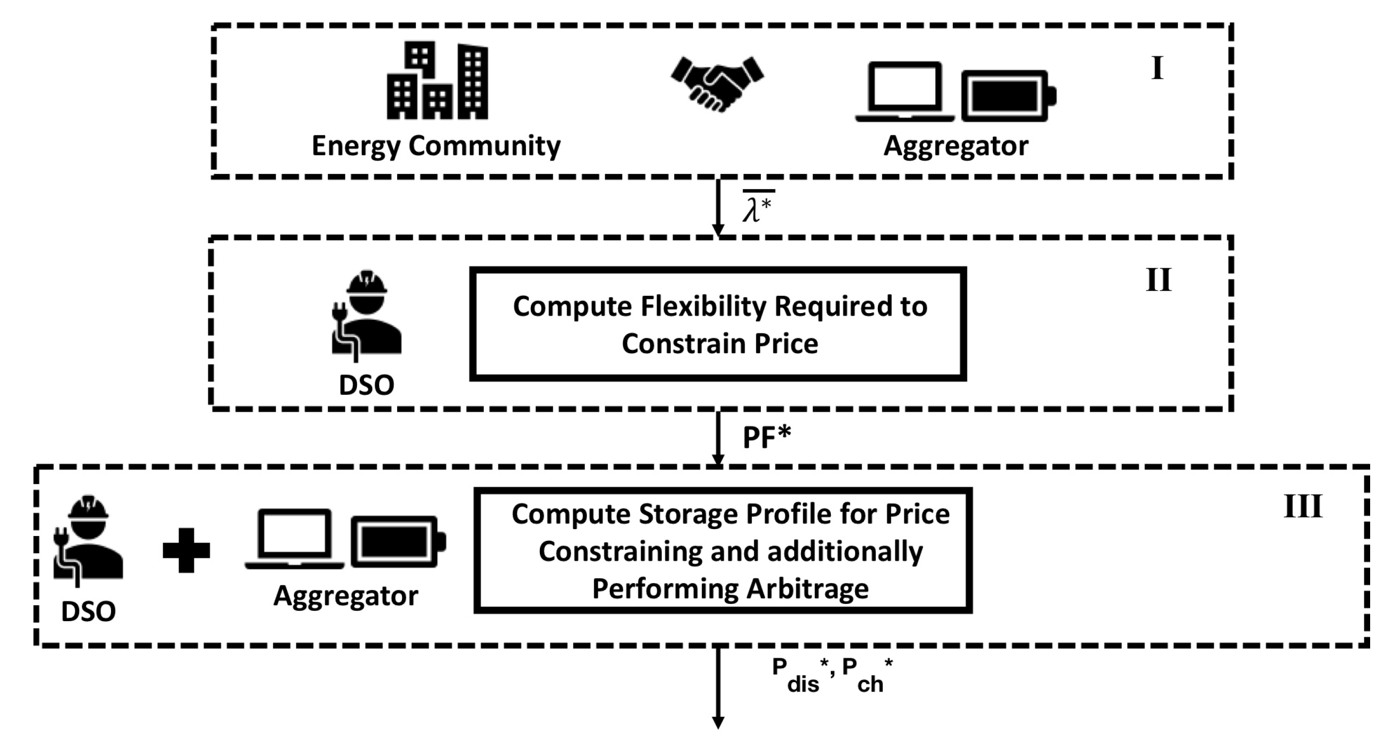
Through Figure 1, we illustrate the information flow for facilitating the proposed coordination mechanism. The point of initiation of this coordination mechanism is the determination of the price limit , which is an essential parameter. This is determined in Step I as presented in Figure 1 and involves a negotiation between the energy community and aggregator. The contract details could include fixed or variable payments by the community to the aggregator. Once the price limit is established, it is shared with the DSO. In Step II, the DSO can include this contracted flexibility in the market clearing by solving Equation (7). This would result in an allocation of the generation and demand, but also the required . The computed volume of required flexible power is then broadcast to the aggregator, who is then contractually obligated to deliver this in real-time. Determination of the optimal storage profile for satisfying the required flexibility is computed in Step III where the DSO and aggregator cooperate for dispatching the storage, thereby ensuring that grid contingencies are mitigated. Once the aggregator provides the required flexibility, it is remunerated for its services by the energy community. Additionally, at intervals when the aggregator is not required to deliver flexible power, it can partake in energy arbitrage to further increase its revenue. In the next section, we will elaborate further on the case study considered for the implementation of our proposed mechanism.
3. Case Study
Section 2 provided the mathematical foundation for constraining price to a certain price limit and for quantifying the flexible power required to achieve it. Additionally, we elaborated on an organizational structure that captured the information flow between actors for the coordination of this flexible power. In this section, we build on these fundamental blocks and apply the proposed mechanism to a case study that focuses on a community of residential consumers who have photovoltaic (PV) arrays integrated with their households and are exposed to high price volatility and price spikes during periods of grid congestion. It must be mentioned that the exact ownership structure and optimal sizing of the PV arrays is out of the scope of our current analysis and will be considered in future work. An energy storage system can be considered as the source of flexibility to reduce price volatility by constraining price to a certain limit. Hence, consumers in this community may decide to buy an energy storage unit collectively to use it during periods of high prices. In principle, these consumers can simply discharge the storage at times of high prices and recharge it when the prices are low. Alternatively, there could be another party that invests in and operates a storage system separately. For such a commercial party, it could be beneficial to discharge during times of congestion as long as it does not resolve the congestion completely (which would reduce the price it gets for its delivered energy). This can be seen as a form of exercising of market power, but it is rational for the storage operator in order to maximize their revenue. The community could make an agreement with the aggregator to pay a fixed yearly fee per unit of energy (€/MWh) to ensure that the price does not exceed a certain price limit . Thus, in the day-ahead market, the aggregator would discharge the storage when the local price in the community would exceed the agreed on price limit.
3.1. Determining the Volume of Required Flexibility
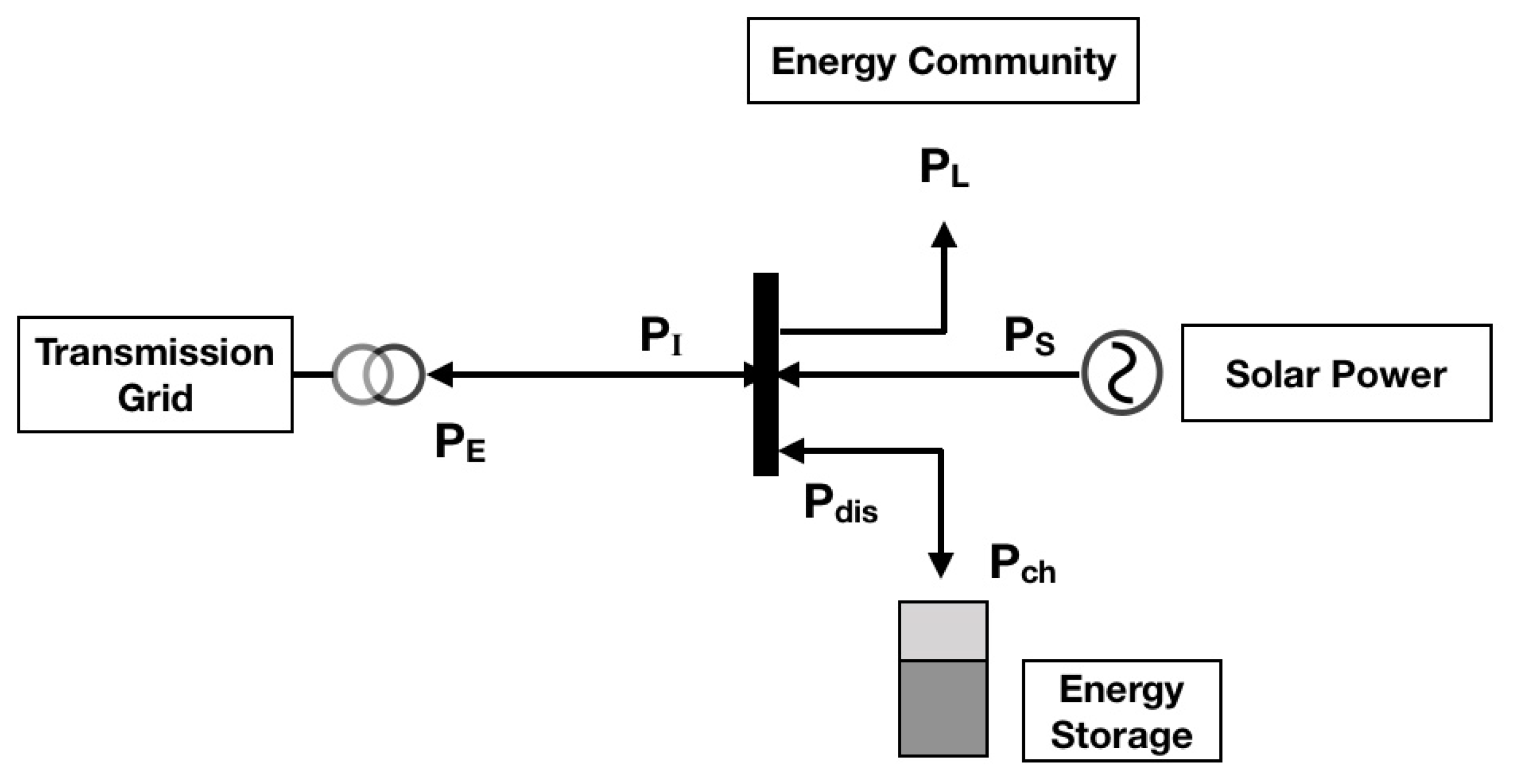
Equation (5) describes the general case of determining the flexibility to cap prices in a multi-node system. For the purpose of our case study, we considered a single node system. In Figure 2, we present our case study that considered a system setup where an energy community was connected to a larger network. To model the price spikes as a result of congestion, we assumed that the load in our distribution network was elastic, with the following quadratic expression describing its utility B:
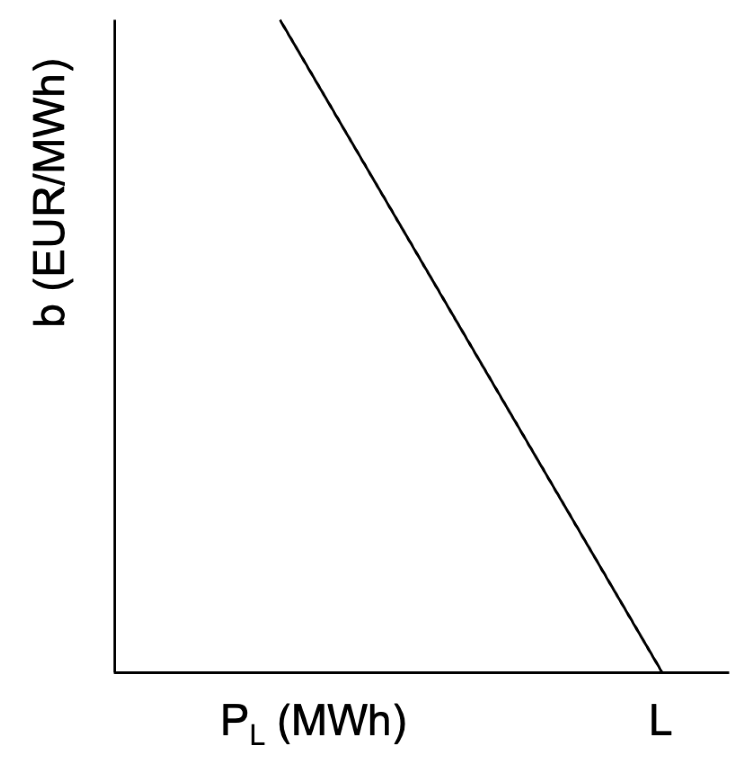
In Equation (8), the utility function is described for an hourly period. The variable b is the marginal utility and is described as a linearly decreasing function of demand, as shown in Figure 3. Furthermore, this marginal utility is comprised of a relationship between the inelastic load L, elastic load , and a coefficient of demand elasticity .
Power can be supplied to the community from the main grid. Alternatively, power supply to the community can be provided through solar generation. Previously, the formulation presented in Equation (7) did not account for power flowing from the distribution grid to the main grid. In this network, we considered the excess of solar power generation to be sold back to the main grid. The flexibility required for capping the local price in the day-ahead market (operating at hourly intervals) experienced by the energy community can be computed as:
subject to:
The variable represents the cost (in €/MWh) of supplying power from the main grid to the energy community and of supplying the excessive power from the community to the larger network. This value is obtained from the wholesale market price. At a given instance, power can either be imported to () or exported from () the energy community. To ensure that the variables and are not simultaneously active, a nominal difference is introduced in the cost terms associated with the two power variables. Equation (9a) presents the power balance equation where and represent the solar generation and flexibility required to constrain the price to the value of , respectively. The solar power is provided at zero marginal cost. At intervals when the market prices are higher than the value of the contractual price limit , the power provision from the energy community to the larger network is set to zero using the constraint (9b). The amount of power that can be supplied from the main grid and power that can be supplied to the main grid are limited by the line capacity and is expressed by . The DSO in its capacity as a regulated market facilitator [42] would have the information about generator and demand bids and the network structure, thereby enabling it to execute the formulation expressed in Equation (9) to determine the flexibility that the aggregator would need to supply.
3.2. Battery Storage as a Flexible Generation Source
The equations presented in Section 2 are general for any type of flexibility. In our case study, the focus is on energy storage as a demand-side flexible resource. To model the storage system, we will introduce additional essential constraints that enrich the formulation as expressed in Equation (7).
3.2.1. Optimal Storage Size
An energy storage system through charging and discharging can provide the flexibility required to constrain the marginal prices. By executing Equation (9), the time series of the required flexibility is determined. An aggregator in order to make an investment decision about the storage capacity would need forecasts about the required flexibility. Then, in order to determine the minimum storage capacity needed by the aggregator to satisfy the time varying signal , the following optimization problem would need to be executed:
subject to:
By executing Equation (10), the optimal energy storage system (ESS) size is determined. In Equation (10), the variable d represents the annualized per unit cost of the storage expressed in €/MWh-year, and is the size of storage. The reason for annualizing the costs of storage is to enable a business feasibility analysis on the basis of comparing investment costs against the yearly operational revenue. Equation (10a) expresses the inter-temporal constraint associated with the operation of the storage system. The variables represents the state of charge, while variables and are the respective variables associated with the discharging and charging of the storage. Equation (10b) is the constraint required for satisfying the required flexibility by discharging the storage. The operation of the storage is governed by its physical characteristics, and the amount of energy charged and discharged from the storage at any instance should not exceed the physical size of the inverter, which is defined as a function of the storage size and a charging/discharging time constant expressed in hours. Note that it is possible that if the storage is inadequately sized, simultaneous charging and discharging of the storage may occur. In order to account for this anomaly, a soft penalty can be introduced in the objective function by adding the expression where is a penalty factor expressed in terms of €/MWh [43].
3.2.2. Providing Flexibility with an Energy Storage System
In the day-to-day operation of the storage, the storage capacity can be reserved to provide the flexible power required for capping the price to the contractual price limit (i.e., provide ). Thus, whenever the price exceeds the price limit, it would be capped, thereby enabling the price hedging functionality. The operation of the storage can be modeled using the following optimization problem:
subject to:
Equation (11) determines the optimal storage charging and discharging profile for satisfying the requested flexibility. Constraint (11b) enforces that the storage discharge provides the required flexibility. It should be noted that the optimization problem specified is in essence a centralized economic dispatch problem. It represents the most efficient outcome that would emerge in a perfectly functioning local market. The solution provides the cost-optimal schedule of charging the energy storage system that still meets the obligations to deliver the contracted flexibility .
As an artifact of our problem description, the price term , is updated to reflect the constrained price , obtained by executing Equation (9). These prices are such that whenever the cost of electricity in the market would exceed the contractual price limit () specified by the community, the prices would be constrained. Equation (11a) reflects the power balancing performed at the community inclusive of the storage charging and discharging. Similar to Equation (9), the amount of power that can be provided to the community from the main grid or vice versa is restricted by the line capacities. Equations (11c)–(11f) represent the operation of the storage system as a flexible resource governed by its physical properties. The size of the storage is computed from Equation (10). Simultaneity may arise in the presented formulation such that mutually exclusive variables of and may be non-zero. This can be accounted for by adding a soft constraint of the form to the objective function. Finally, given the close interaction between the power flow and storage operation, this step is executed jointly by the DSO and aggregator, thereby mitigating additional grid contingencies.
3.3. Flexibility and Arbitrage With an Energy Storage System
The problem formulation in the previous subsection ensures that the energy storage system always delivers the contracted flexibility. However, it may be economically overly conservative, since there could be additional opportunities to perform energy arbitrage, i.e., to charge and discharge the storage based on price differences over time, while still meeting the obligations of when needed. In order to account for this, we only have to change Constraint (11b) into the following:
This means that the storage is left free to perform additional charging and discharging cycles as long as it delivers when needed, i.e., when it is greater than zero.
3.4. Arbitrage Only with an Energy Storage System
As a useful comparison case, we also present results of a case where the storage is only used for arbitrage. This setup is exactly as described by Equation (11), but without Constraint (11b). In this case, the storage will be used to minimize the costs in the distribution grid, thereby flattening the price. However, as there is no notion of a price limit, the subsequent flexibility quantification will not be computed, thereby making the formulation incapable of guaranteeing that price does not exceed the community-specified limit.
3.5. Economic Evaluation
In this subsection, we shift our focus towards the economic analysis of our proposed formulation. The basis of this analysis is the contractual arrangement made between the energy community and the aggregator. By controlling the energy storage, the aggregator provides the required flexibility for constraining the price experienced by the consumers. For the provision of this flexibility, the energy community is contractually bound to provide remuneration to the aggregator. We make a distinction between the income, costs, and operating revenue for the purpose of our analysis. Income refers to the positive cash in-flow for the aggregator, while costs pertain to the cash out-flow that the aggregator incurs for charging the storage. Finally, operational revenue is the term used to denote the net value computed by taking the difference between the income earned and costs incurred by the aggregator.
Without the consideration of a premium, the aggregator income from hedging alone, i.e., the provision of flexibility to constrain price, is expressed through Equation (13) as:
where denotes the time-steps in which , i.e., in which flexibility was provided (Since energy is priced in €/MWh, Equation (13) is dimensionally not correct, and we should multiply by the simulation time-step. Since we used a simulation time-step of one hour, we omit if for brevity). The variable denotes the constrained marginal price.
For maintaining a sufficient state of charge and for satisfying the flexibility requests over multiple time periods, the aggregator would need to charge the storage, for which it would incur an operational expenditure (OPEX). The corresponding OPEX is thus:
where denotes the time-steps in which the storage charges in order to be able to satisfy the flexibility requests during the periods defined by .
Hence, the net revenue earned by the aggregator from hedging is represented as:
Additionally, the aggregator can earn revenue from arbitrage. The net revenue from arbitrage is defined as:
For computing the total operating revenue for the aggregator, we compute:
To participate in the price constraining and arbitrage, a decision needs to be made regarding investing in assets, particularly the storage system. The annualized capital expenditure (CAPEX) for this is investment is given by:
where D denotes the total capital cost per MWh and denotes the annuity factor:
where is the lifetime of the storage and is the interest rate.
In the case when , a net positive business potential for the given contractual agreement can be realized by the aggregator.
4. Simulations and Results
Through quantitative analysis, we illustrate how the formulation presented in Section 3 facilitates the computation of the required flexibility for reducing the impacts of price volatility and price spikes. In this section, we first introduce the data used for the simulation followed by the analysis of the results.
4.1. Simulation Setup
We performed numerical simulations to illustrate the case study. To the extent possible, we used realistic data of demand, wholesale prices, solar generation, and storage costs. These data are elaborated later in this section. The value of the variable was based on the wholesale market data for the year 2017, which was obtained from the Amsterdam Power Exchange [44]. High price volatility was observed for this year with the prices varying as much as ±€60/MWh between two consecutive hours in the day-ahead market. The power output of the photovoltaic (PV) systems depends on the solar irradiance of the given region. These irradiance values are converted into solar generation values (in MW) through the following formulation:
where is then taken as the average for the entire hour. From Equation (20), it is clear that the solar power generation depends on the area that solar panels cover (A), the solar panel efficiency (r), and the performance ratio () that accounts for losses. For the purpose of our simulation, we set the value as (A= 25,000 m), , and . The hourly averaged irradiance values (converted to MW/m) were obtained from the Dutch meteorological institute Koninklijk Nederlands Meteorologisch Instituut (KNMI) [45].
In the case study, we focused on an energy storage system to provide the contracted flexibility. After reviewing the different storage options presented in [46], zinc bromide energy storage was selected due to its economic viability. The cost of this storage system was annualized to represent a yearly investment decision. Using a total capital cost (TCC) of €170/kWh, a lifetime of 20 years from [46], and a near-zero interest rate, the annualized cost of storage as given by Equation (19) amounted to €8500/MWh-year. This storage was assumed to have an efficiency , and a time constant of = 2 h was used as an estimation of the converter size. Finally, to ensure that simultaneous charging and discharging of the storage did not occur, a penalty factor of = €1000/MWh was introduced.
The demand data used for our simulation were obtained from [47]. These data emulated the load profiles for 5000 residential consumers for the Netherlands and were characteristic of medium voltage (MV) distribution grids. It was assumed that the loads were tuned to maximize their utility as expressed in Equation (8). In Equation (8), the coefficient = €1000/MWh. As previously mentioned, power could be supplied to this energy community either from the main grid with the line capacity as 2 MW or from solar generation by the PV arrays. Essential to our proposed formulation was the presence of a contractually agreed price, and in the simulation of our case study, this value was set to = €50/MWh. This value was assumed to be constant for the entire year. For simulating the case study, we used the IPOPT solver through the Pyomo package [48] provided in Python 3.7.
4.2. Simulation Results
Using the simulation setup described in Section 4.1, we executed the formulation presented in Section 3. The efficacy of the proposed coordination mechanism was illustrated by comparing a scenario in which there was no flexibility to a scenario in which flexibility was provided from an energy storage system. This section is concluded by performing an economic analysis that investigates the optimal storage size, the cost of storage investment, and the operational revenue earned by the aggregator assuming different contractual price limits. The aim of this analysis was to determine which price limits would result in feasible business cases.
4.2.1. Reference Case
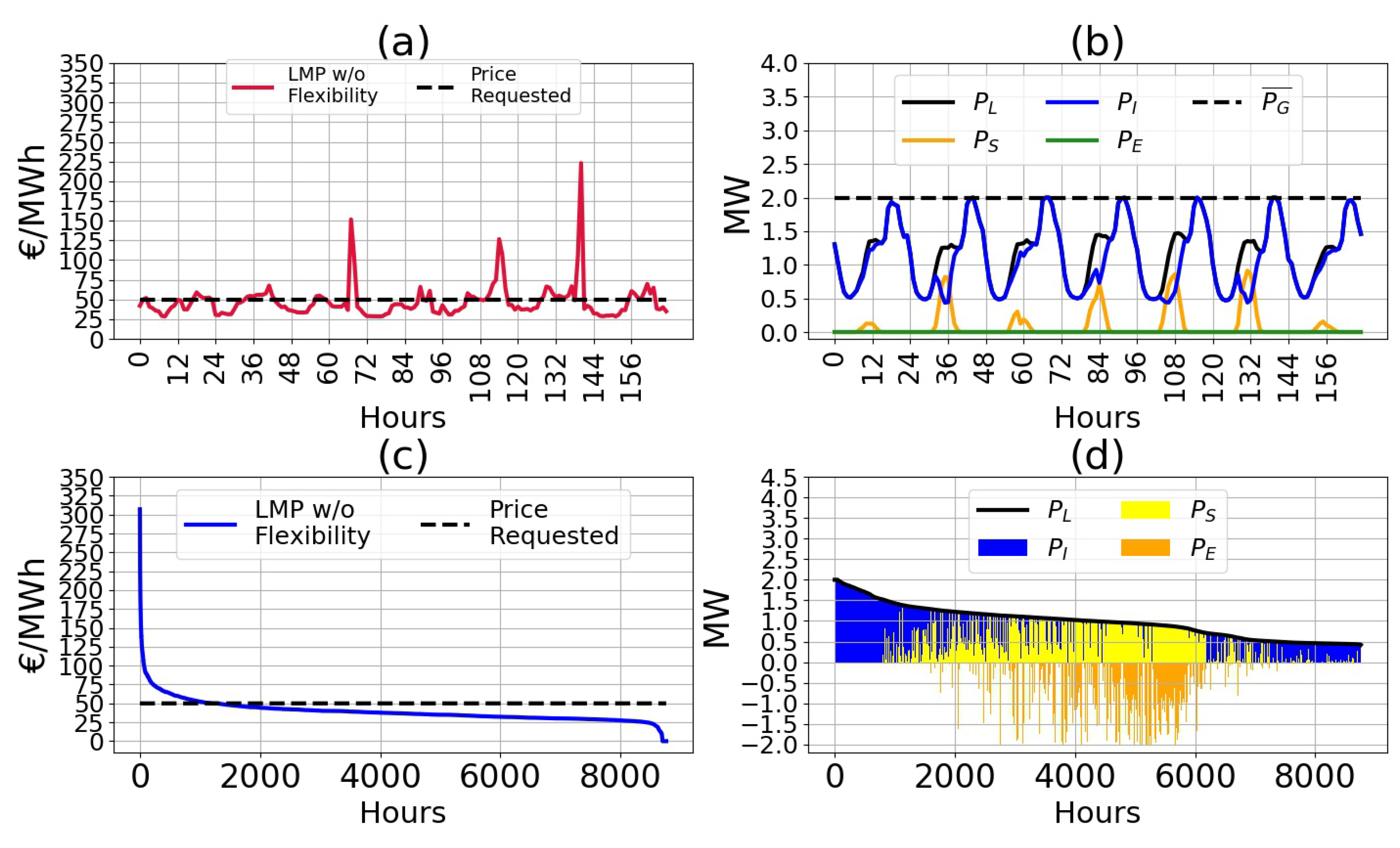
In the reference situation, there was no flexibility in the distribution grid. Due to varying wholesale prices and local congestion, there was a certain level of price volatility. Figure 4a,b represents the price values and generation and load profiles for a typical week, respectively. Price in this scenario exceeded the indicated limit of €50/MWh either because the wholesale price exceeded this level or because of the grid capacity of 2 MW was reached. In Figure 4c, the price duration curve is presented, which illustrates the price experienced by the energy community, organized in descending order of magnitude. As can be observed, the price rise could be as high as €300/MWh, and this high price could be experienced for a considerable duration of time. Furthermore, prices in the price duration curve are higher than the example price limit of €50/MWh for approximately 1500 h. For a few hours during the year, the demand could be satisfied completely by solar power. This caused the marginal price of power to be €0/MWh.
Figure 4d presents the generation and demand profiles for the year and is illustrated through a load duration curve. A load duration curve depicts the relationship between demand and supply in a descending order of demand. In this figure, power can be supplied from solar power (yellow) or can be imported from the main grid (blue) to satisfy the demand (black). Alternatively, an excess of solar power generation can be exported (orange) to the main grid and is represented using a negative sign. As the generation of solar energy depends on the magnitude of solar irradiance, which is variable, the demand might not always be satisfied through solar alone. From the load duration curve, it was observed that solar generation was mostly available during the mid-load hours, i.e., between 1.0 MW and 1.5 MW. In the event that no solar power was available, the demand would need to be satisfied by importing power from the main grid, which in turn was constrained by the line limit. However, for majority of the hours, the power import from the main grid and solar power would combine to satisfy the demand, with rules of economic dispatch taking precedence.
4.2.2. Constraining Price Using Energy Storage
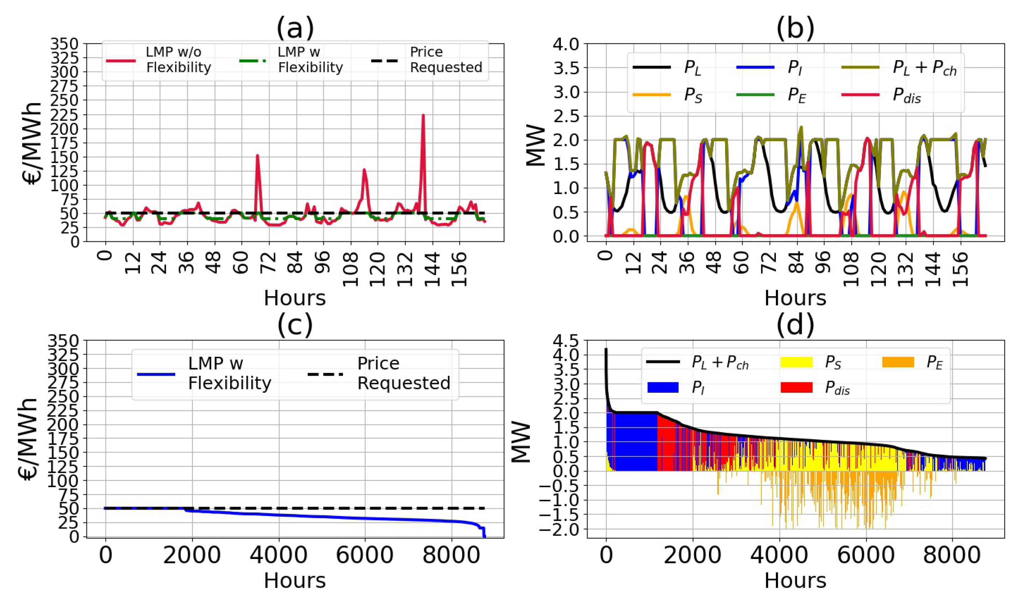
The coordination mechanism for reducing price volatility and price spikes is demonstrated using Figure 5. The results from the implementation of our proposed formulation over a week are presented through Figure 5a,d. From Figure 5a, it can be observed that the marginal price without flexibility provision (red) could exceed the desired price limit. This occurred for a few instances in the given week. At these instances, the DSO issued a request for flexibility to the aggregator on behalf of the energy community.
This requested flexibility was satisfied by discharging of a storage system as described in Equation (Section 3.2.2). Figure 5b depicts the storage operational profile in addition to generation and demand profiles. Once the storage had discharged to constrain the price, it needed to charge in order to constrain price over multiple periods. Additionally, the aggregator could also participate in arbitrage (not shown in this figure). For charging, the aggregator needed to determine the economically beneficial time periods. From Figure 5b, it is observed that charging mostly took place during the night when price was low. Furthermore, the aggregator dispatched the storage in coordination with the DSO, thereby avoiding additional grid contingencies. The combined load and charging used the entire grid capacity of 2 MW. Finally, charging of the storage resulted in a net increase in the local demand. This subsequently resulted in an increase in marginal price as compared to the case without flexibility and can be seen in Figure 5a, where the green line lies above the red line during the low price periods.
The price for the entire year considering the price hedging mechanism and the operation of energy storage as a flexible resource is presented in Figure 5c. It is observed that by discharging the storage, the price was capped at for the entire year, which exhibited the effectiveness of our proposed mechanism. The net increase in relative price experienced by the energy community due to charging occurred for a period of approximately 1000 h when the price was most favorable. Additionally, the price increase in most cases was nominal.
The generation, demand, storage, and grid exchange for the whole year are summarized in Figure 5d. Storage discharge mostly took place during hours when the demand was roughly between 1.5 MW and 2 MW. Comparing Figure 4c and Figure 5c, it can be observed that these were actually the hours with the highest loads in the distribution grid. During the periods of storage charging, the storage would utilize all of the remaining (other than the consumer demand) available 2 MW capacity of the grid connection. For a small amount of hours, the combined load in the grid would exceed 2 MW. These were the hours when either the storage discharging or solar generation complemented the imports from the main grid.
4.2.3. Economic Analysis of Contractual Arrangements
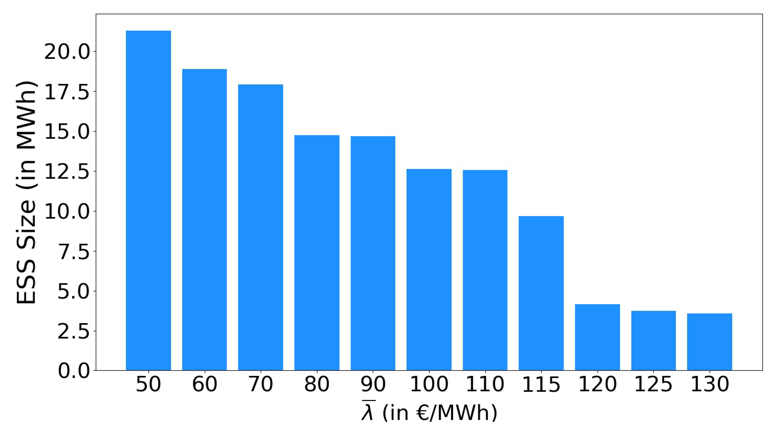
The economic analysis of different contractual arrangements is performed in this subsection. Using the formulation presented in Equation (10), we computed the optimal size of the ESS required to constrain the price to the contractual limit of . Figure 6 presents the relation between the values of and the optimal size of the storage system. It can be observed that as the price limit was relaxed, the size of the storage required significantly decreased.
The resulting size of the ESS depended on the number of consecutive hours that the marginal price exceeded the value of , which in turn corresponded to the required depth of discharge and charge that the storage must sustain. For the purpose of our exploratory analysis, the step size in terms of the contractually agreed on price limit was €10/MWh for the contractual price ranging between €50/MWh and €110/MWh. For higher values, the step size was then further granulated to reflect a value of €5/MWh. From the value of €50/MWh to €70/MWh, a steady drop in storage capacity from 21.3 MWh to 17.93 MWh was observed for constraining the marginal price. However, a nominal decrease in storage capacity was realized when the value of was increased from €80/MWh to €90/MWh and then again from €100/MWh to €110/MWh. This was because for the year, the number of consecutive hours in which the price realized was between these pairs of values of was scarce. Finally, as the value of increased beyond the value of €115/MWh, the storage capacity required for constraining marginal price drastically decreased.
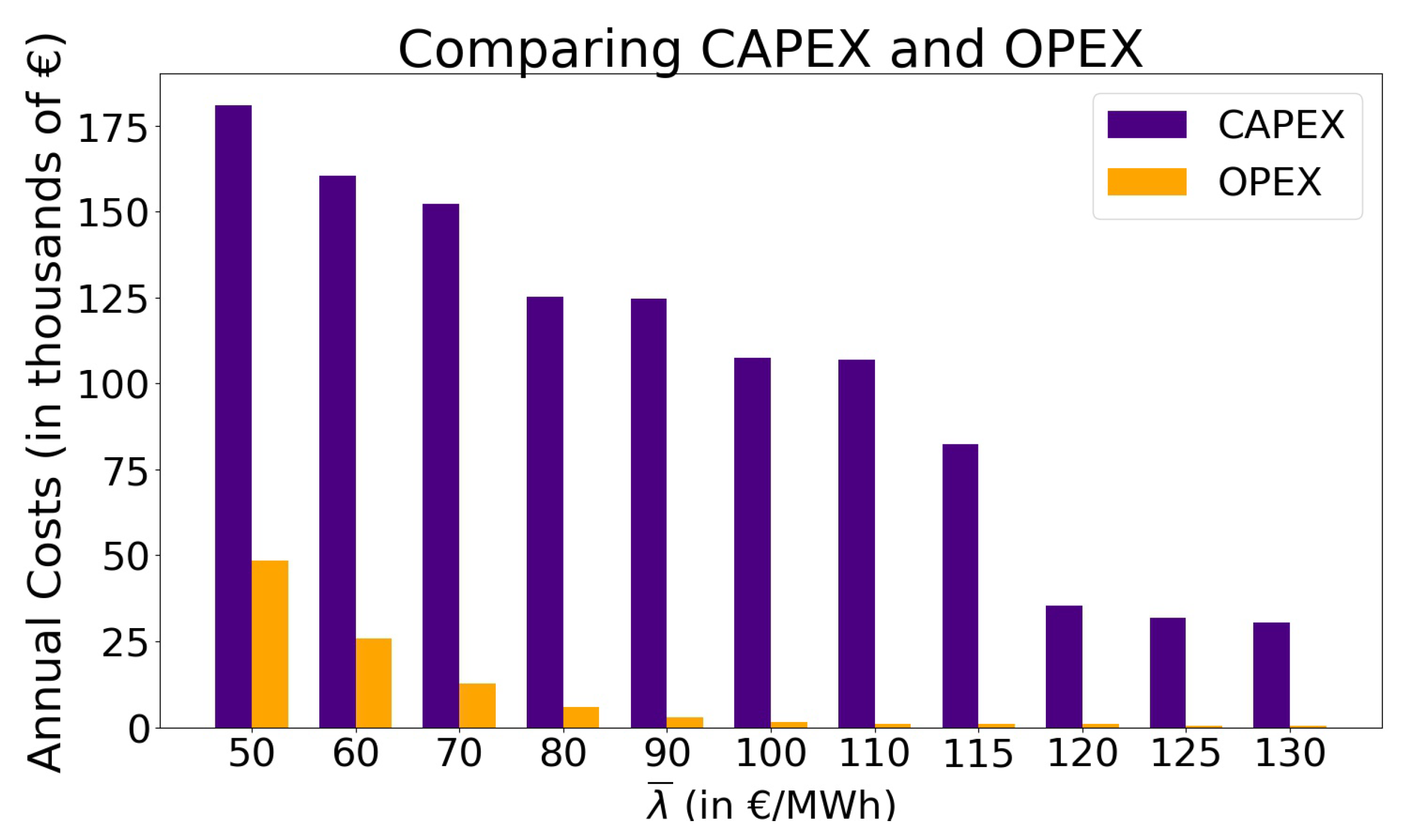
Figure 7 presents a comparison between the capital and operational expenditure incurred by the aggregator to satisfy its contractual obligations. CAPEX values are related to the investment decision that the aggregator needs to make. The total annualized investment cost for the storage system is computed using Equation (18). In accordance with Figure 6, we can observe that as the value of was relaxed, the annualized costs of the storage system significantly decreased. The OPEX of the aggregator is related to the charging of the ESS and is computed using Equation (14). Charging the ESS during periods of low electricity price ensured that it was able to discharge when the marginal price needed to be constrained. As expected, as the price limit for the community was increased, there would be a decrease in the cost of charging due to reduced instances of when flexibility requests were issued. For example, when the price limit for the energy community was aggressive, i.e., when the value of €50/MWh, then for that case, the annualized investment cost for the aggregator was 181,050/year. Correspondingly, given the frequency of the number of hours where the prices realized in the day-ahead market were higher than the value of , the cost of charging was 48,490.33. Comparatively, when the value of €125/MWh, then the investment and charging costs were significantly lower with values of 31,705/year and 958.714, respectively.
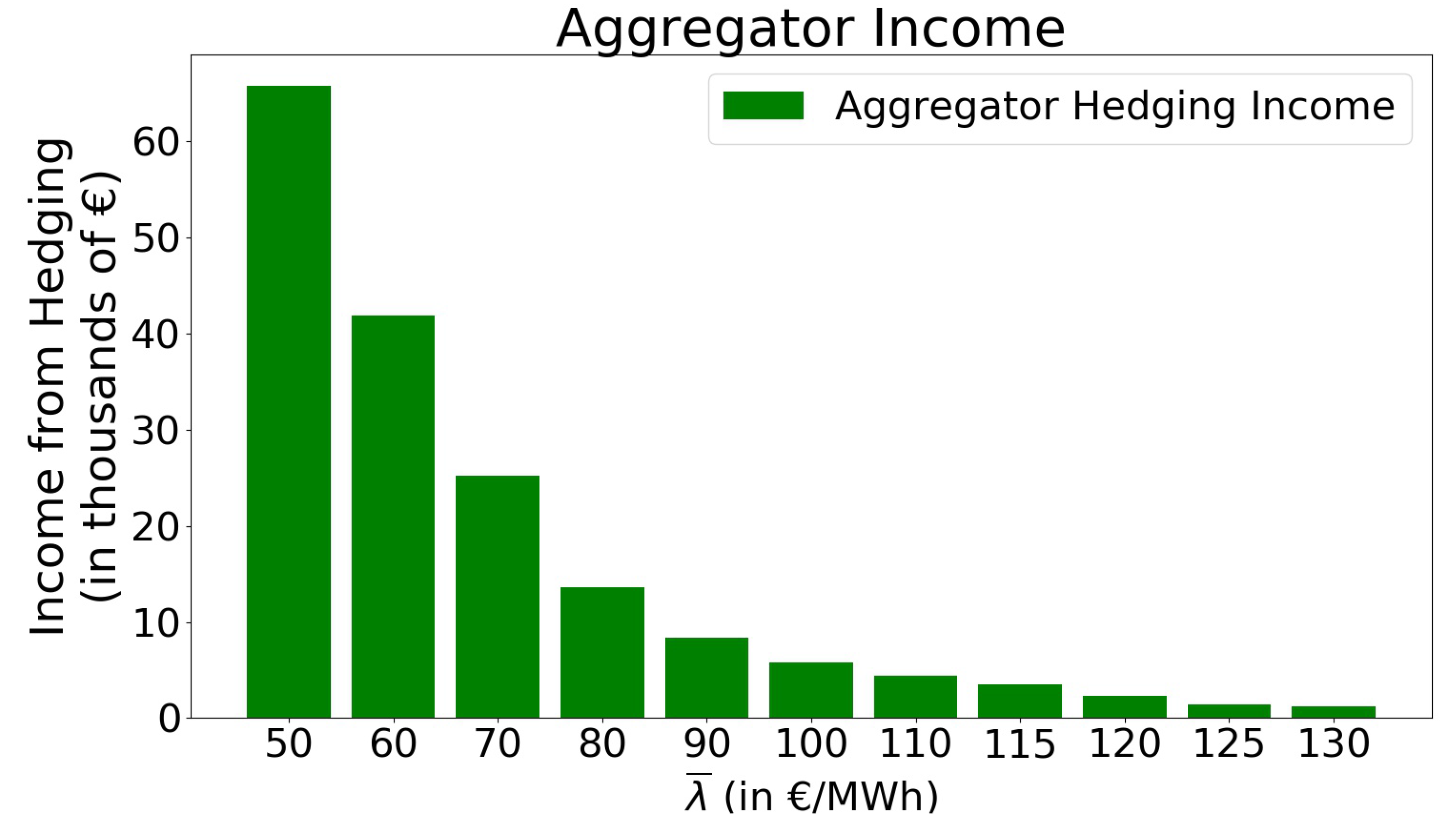
As part of the contractual agreement, the aggregator earns an income from the payments made by the energy community for constraining the price. The income from hedging is defined by Equation (13) and is shown in Figure 8. This income decreased sharply for higher price limits. Although the price at which the flexibility was sold increased, the number of hours in which the flexibility was provided fell more rapidly. As a result, the income from hedging (the product of the number of hours flexibility was provided, and the price limit (see Equation (13))) decreased. For example, with €50/MWh, the aggregator income was 65,760.55, while at €125/MWh, it was only 1444.75.
The aggregator could earn additional revenue by partaking in arbitrage during the periods when it was not required to satisfy flexibility requests. To perform arbitrage, the aggregator participated in the wholesale electricity market as a price-taker, charging the storage when the price was low and selling electricity by discharging when the price was high. However, instances may arise when the aggregator was required to forgo arbitrage opportunities in order to satisfy its contractual obligations. This in turn limited the revenue potential from performing arbitrage and could be observed clearly for when the price limits were aggressive.
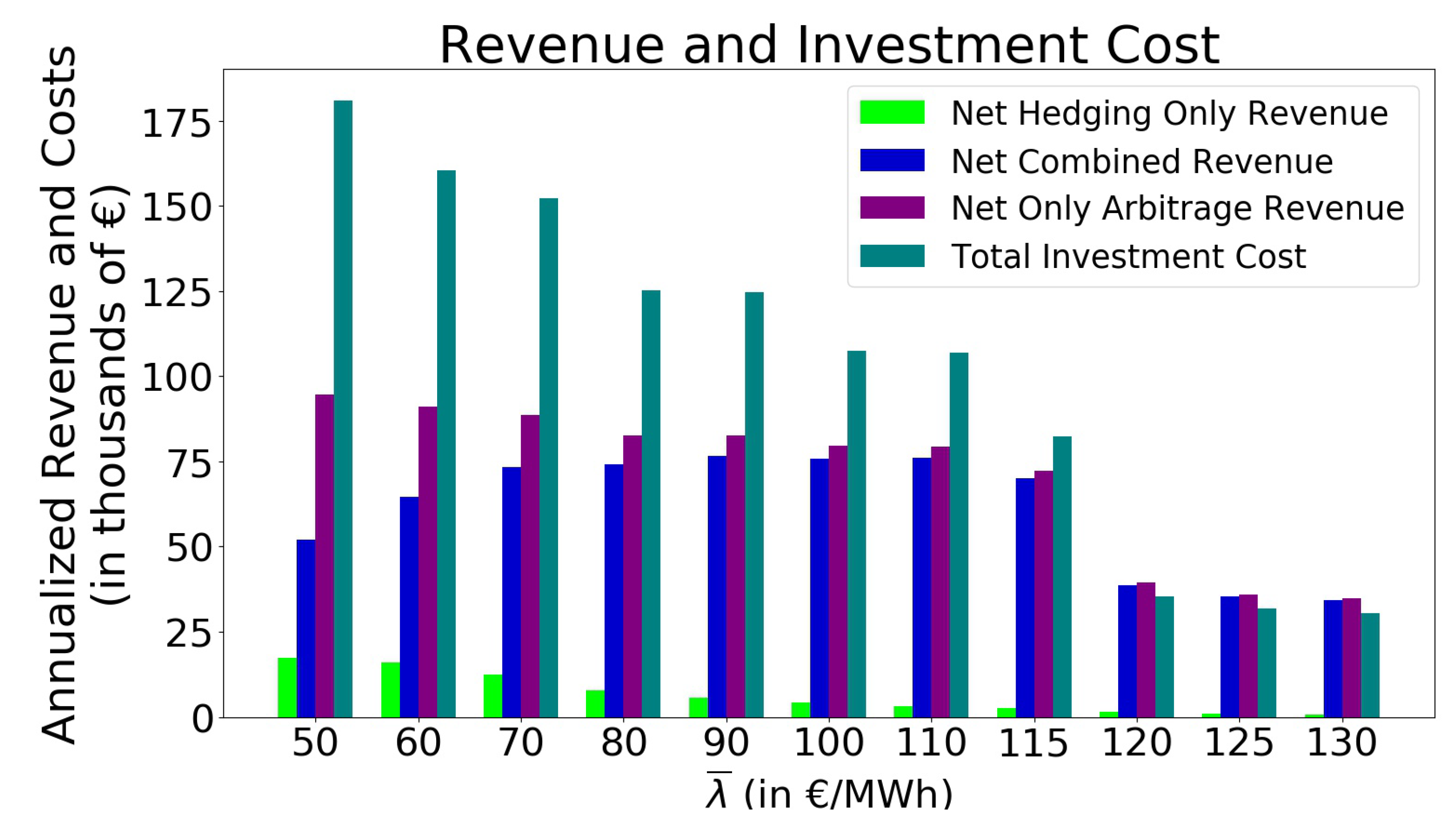
While increasing the price limit resulted in diminishing return from hedging, the upside was that the storage had more opportunities for arbitrage as the frequency with which Constraint (12) was to be executed decreased. Figure 9 shows the net operational revenue from combined arbitrage and hedging (blue), net hedging revenue only (green) with different price limits, as well as corresponding annualized storage investment costs (teal). As a reference, in Figure 9, we also consider the revenue potential if an aggregator were to perform only arbitrage (purple) given the same size of storage. Indeed, Figure 9 shows that in the combined hedging and arbitrage case, the arbitrage revenue increased when the price limits were relaxed. In fact, they approached the arbitrage revenue of the arbitrage-only case. This made sense, when realizing that the only difference between these two cases was that Constraint (12) forced the storage to provide flexibility . At more relaxed price limits, this constraint became increasingly inactive, and the two cases became increasingly alike. The difference between the purple and the blue bars in Figure 9 could thus be considered as the cost of imposing a price limit.
A key observations can be drawn from the analysis of Figure 9. The revenue potential from hedging and arbitrage was governed by the size of the storage system. The storage in turn was sized such that it was able to constrain the marginal price to the contractual limits throughout the year. Figure 9 also makes clear that with the data used for this case study, there was only a positive business case for values of the price limit of €120/MWh or higher. At the price limit of €120/MWh, the corresponding size of the ESS required was 4.17 MWh, and the annualized storage investment costs and combined hedging and arbitrage revenue were 35,431.4/year and 40,118.06/year, respectively. Thus, at higher price limits, the storage size and its corresponding costs decreased rapidly while the revenues from storage operation fell less sharply. In other words, a relatively small sized storage was able to provide flexibility and arbitrage for a small number of hours, but against very favorable prices.
For this case study, the net revenue from hedging alone was too low for a positive business case. However, we did not consider a premium or fixed fee that the provider of flexibility would receive. In principle, since local price was reduced for the entire grid, a risk-neutral consumer could be expected to pay the same amount of money compared to the situation without flexibility.
4.2.4. Comparative Analysis of Combined Hedging and Arbitrage and Arbitrage Alone
As previously mentioned, the aggregator can integrate with the energy community without entering into a flexibility contract. In this case, the aggregator would operate the storage purely to leverage from the price volatility by performing arbitrage. From Table 1, it can be observed that the main benefit of our proposed formulation was that it was able to constrain price to the community-specified limit. In contrast, the storage operating purely for arbitrage was unable to guarantee a price limit. For our comparative analysis, the size of storage for each comparison scenario was kept constant. From Table 1, it can be noticed that when there was an aggressive price limit = €50/MWh, then while the difference between the maximum price in the two cases compared was high, the maximum price in the arbitrage only case was the lowest compared to the other price limit scenarios. This was because the given price limit of €50/MWh required a larger storage size to constrain the price successfully.
Furthermore, it could be observed that as the price limit was relaxed, the difference in the maximum price for the two cases being compared also decreased. However, the trade-off of our proposed formulation was that placing a price cap resulted in a reduced overall system benefit. Subsequently, the revenue for the aggregator reduced as compared to a situation in which the aggregator performed arbitrage alone. Additionally, we observed that total system benefits (utility minus costs) were only slightly (%) higher in the arbitrage only case. This showed that imposing an extra constraint on the system indeed led to a lower optimum, but the costs in both cases were almost comparable.
5. Conclusions
In this paper, we presented a coordination mechanism that was used to reduce price volatility and price spikes in electricity systems. The novelty of this mechanism was that it applied an explicit constraint on price, which was generally an output of an optimal power flow and not known a priori. Our proposed approach used duality theory for quantifying the flexible power required to constrain price to the desired limit. An institutional arrangement for the required coordination mechanism was presented that illustrated the information and money flow between consumers, a market facilitator, and the operator of a flexible resource.
The concept presented was illustrated with a case study of an energy community located in the distribution grid that faced increasing price volatility and price spikes due to wholesale price and local congestion. An aggregator entered into a flexibility contract with the community, thereby operating an energy storage to satisfy flexibility requests and constrain price. Additionally, at instances when there were no flexibility requests, the aggregator could participate in energy arbitrage. A techno-economic analysis from the aggregator’s perspective was considered in this paper, where the aggregator’s revenue from the combination of arbitrage and hedging, under different price limits, was compared against the storage investment cost. Results indicated that strict price limits restricted the level of volatility in the local electricity market, and hence, a trade-off was observed in the aggregator’s revenue when comparing the combined arbitrage and hedging case with the arbitrage only case. Furthermore, from the techno-economic analysis, it was observed that the business case for the storage system depended strongly on the price limit in the grid. For the case study investigated, a business case was realized as the value of increased over €120/MWh. Finally, a comparison with the arbitrage-only case showed that the reduction in overall system benefit of imposing an additional constraint on the system was modest.
In conclusion, this paper serves as a preliminary proposal for physical hedging in distribution grids, and future research could provide insights on several aspects that were not addressed here. Firstly, we considered the flexibility contract to have a constant price limit for the entire year. The shortcoming of such a contract is that when the price of electricity in the market is low, the aggregator is not able to generate revenue through hedging. Alternatively, periods may exist when the price of electricity is consecutively high for long periods. Since the storage capacity sizing is directly related to the number of consecutive hours for which the market price is higher than the contractual price limit, it will result in a requirement for large storage units, which are expensive. Assigning a time-varying value for the price limit can aid in alleviating this issue. Secondly, we only considered an energy storage system as a potential source of flexibility in our case study, but it would be interesting to investigate demand response technologies like electric vehicles or flexible heating/cooling systems. This is because the electrification of transport and heating and could contribute to grid congestion, thereby resulting in additional price spikes. Thirdly, we treated everything in a deterministic framework, where full knowledge of future price and demand was assumed. Uncertainty should be considered to get a more realistic estimate of the operation and economics of the system. Finally, our presented formulation is readily extendable to larger systems with multiple nodes and possibly higher voltage levels such as the transmission grid. Thus, additional insights from our approach could be generated including the analysis of the computational feasibility of the approach.
Author Contributions
Conceptualization, S.C., K.B., R.V., and L.D.V.; methodology, S.C., R.V., M.C., and Z.L.; software, S.C. and R.V.; validation, S.C. and R.V.; formal analysis, S.C. and K.B.; writing, original draft preparation, S.C.; writing, review and editing, R.V., K.B., M.C., L.D.V., and Z.L.; supervision, R.V., K.B., M.C., and Z.L. All authors read and agreed to the published version of the manuscript.
Funding
This work received funding from the European Union’s Horizon 2020 research and innovation program under the Marie Sklowdowska-Curie Grant agreement No. 675318 (INCITE).
Conflicts of Interest
The authors declare no conflict of interest.
Abbreviations
The following abbreviations are used in this manuscript:
| T | length of simulation time period (hours) |
| t | discrete time interval (hours) |
| B | Load utility (€) |
| b | marginal load utility (€/MWh) |
| L | inflexible load (MW) |
| d | annualized per unit cost of energy (€/MWh-year) |
| C | annualized investment cost (/year) |
| D | total capital cost per unit of energy (€/MWh) |
| TCC | total capital cost |
| A | solar panel area (m) |
| r | solar panel efficiency |
| H | average hourly solar irradiance (MW/m) |
| DSO | distribution system operator |
| TSO | transmission system operator |
| ISO | independent system operator |
| ESS | energy storage system |
| LMP | locational marginal prices (€/MWh) |
| CAPEX | capital expenditure (€) |
| OPEX | operational expenditure (€) |
| power generation from generator i(MW) | |
| power demand (MW) | |
| maximum power demand (MW) | |
| minimum power demand (MW) | |
| marginal cost of generator i (€/MWh) | |
| marginal price of electricity (€/MWh) | |
| dual variable associated with upper bound generator i (€/MWh) | |
| maximum generation from generator i (MW) | |
| contractual price limit (€/MWh) | |
| flexibility provided at node i (MW) | |
| phase angle at bus i (degrees) | |
| reactance between nodes i and j () | |
| line flow limit from bus i to bus j (MW) | |
| contractual price limit at bus i (€/MWh) | |
| set of all nodes in the network | |
| set of all lines in the network | |
| flexibility required at node k to constrain prices (MW) | |
| coefficient of demand elasticity (/MWh) | |
| cost of importing to and exporting power from the energy community obtained from wholesale market price (€/MWh) | |
| power imported to the energy community from the main grid (MW) | |
| power exported from the energy community to the main grid (MW) | |
| solar power generation (MW) | |
| size of energy storage (MWh) | |
| coefficient of storage discharging | |
| coefficient of storage charging | |
| storage charging and discharging time constant | |
| penalty factor for preventing simultaneity (€/MWh) | |
| income from flexibility provision for constraining price (€) | |
| net revenue from hedging (€) | |
| constrained marginal price (€/MWh) | |
| cost of charging for providing flexibility to constrain price (€) | |
| time-steps in which the storage charges for being able to provide hedging functionality (hours) | |
| net operational revenue from arbitrage (€) | |
| net operational revenue from hedging and arbitrage (€) | |
| optimal storage size (MWh) |
References
- Koirala, B.P.; Koliou, E.; Friege, J.; Hakvoort, R.A.; Herder, P.M. Energetic communities for community energy: A review of key issues and trends shaping integrated community energy systems. Renew. Sust. Energ. Rev. 2016, 56, 722–744. [Google Scholar] [CrossRef] [Green Version]
- Parra, D.; Swierczynski, M.; Stroe, D.I.; Norman, S.A.; Abdon, A.; Worlitschek, J.; O’Doherty, T.; Rodrigues, L.; Gillott, M.; Zhang, X.; et al. An interdisciplinary review of energy storage for communities: Challenges and perspectives. Renew. Sust. Energ. Rev. 2017, 79, 730–749. [Google Scholar] [CrossRef]
- Holstenkamp, L.; Kahla, F. What are community energy companies trying to accomplish? An empirical investigation of investment motives in the German case. Energy Policy 2016, 97, 112–122. [Google Scholar] [CrossRef]
- Moret, F.; Pinson, P. Energy Collectives: A Community and Fairness Based Approach to Future Electricity Markets. IEEE Trans. Power Syst. 2019, 34, 3994–4004. [Google Scholar] [CrossRef] [Green Version]
- Tabors, R.; Caramanis, M.; Ntakou, E.; Parker, G.; Van Alstyne, M.; Centolella, P.; Hornby, R. Distributed Energy Resources: New Markets and New Products. In Proceedings of the 50th Hawaii International Conference on System Sciences, Hilton Waikoloa Village, HI, USA, 4–7 January 2017. [Google Scholar]
- Meng, F.; Chowdhury, B.H. Distribution LMP-based economic operation for future Smart Grid. In Proceedings of the IEEE Power and Energy Conference at Illinois, PECI, Urbana, IL, USA, 25–26 February 2011. [Google Scholar]
- Li, R.; Wu, Q.; Oren, S.S. Distribution locational marginal pricing for optimal electric vehicle charging management. IEEE Trans. Power Syst. 2014, 29, 203–211. [Google Scholar] [CrossRef] [Green Version]
- Liu, Z.; Wu, Q.; Oren, S.S.; Huang, S.; Li, R.; Cheng, L. Distribution locational marginal pricing for optimal electric vehicle charging through chance constrained mixed-integer programming. IEEE Trans. Smart Grid. 2018, 9, 644–654. [Google Scholar] [CrossRef] [Green Version]
- Faqiry, M.N.; Edmonds, L.; Wu, H. Distribution LMP-based Transactive Day-ahead Market with Variable Renewable Generation. unpublished.
- Astaneh, M.F.; Chen, Z. Price volatility in wind dominant electricity markets. In Proceedings of the IEEE EuroCon, Zagreb, Croatia, 1–4 July 2013. [Google Scholar]
- McConnell, D.; Forcey, T.; Sandiford, M. Estimating the value of electricity storage in an energy-only wholesale market. Appl. Energy 2015, 159, 422–432. [Google Scholar] [CrossRef]
- Yang, I.; Ozdaglar, A.E. Reducing electricity price volatility via stochastic storage control. In Proceedings of the American Control Conference, Boston, MA, USA, 6–8 July 2016. [Google Scholar]
- Pereira, J.P.; Pesquita, V.; Rodrigues, P.M. The effect of hydro and wind generation on the mean and volatility of electricity prices in Spain. In Proceedings of the 14th International Conference on the European Energy Market (EEM), Dresden, Germany, 6–9 June 2017. [Google Scholar]
- Higgs, H.; Lien, G.; Worthington, A.C. Australian evidence on the role of interregional flows, production capacity, and generation mix in wholesale electricity prices and price volatility. Econ. Anal. Policy 2015, 48, 172–181. [Google Scholar] [CrossRef] [Green Version]
- Rintamäki, T.; Siddiqui, A.S.; Salo, A. Does renewable energy generation decrease the volatility of electricity prices? An analysis of Denmark and Germany. Energy Econ. 2017, 62, 270–282. [Google Scholar] [CrossRef] [Green Version]
- Ketterer, J.C. The impact of wind power generation on the electricity price in Germany. Energy Econ. 2014, 44, 270–280. [Google Scholar] [CrossRef] [Green Version]
- Bradbury, K.; Pratson, L.; Patiño-Echeverri, D. Economic viability of energy storage systems based on price arbitrage potential in real-time U.S. electricity markets. Appl. Energy 2014, 114, 512–519. [Google Scholar] [CrossRef]
- Zakeri, B.; Syri, S. Value of energy storage in the Nordic Power market - Benefits from price arbitrage and ancillary services. In Proceedings of the 13th International Conference on the European Energy Market, EEM, Porto, Portugal, 6–9 June 2016. [Google Scholar]
- Ni, L.; Wen, F.; Liu, W.; Meng, J.; Lin, G.; Dang, S. Congestion management with demand response considering uncertainties of distributed generation outputs and market prices. J. Mod. Power Syst. Cle 2017, 5, 66–78. [Google Scholar] [CrossRef] [Green Version]
- Menniti, D.; Pinnarelli, A.; Sorrentino, N.; Burgio, A.; Belli, G. Management of storage systems in local electricity market to avoid renewable power curtailment in distribution network. In Proceedings of the 2014 Australasian Universities Power Engineering Conference, AUPEC, Perth, Australia, 28 Septembe–1 October 2014. [Google Scholar]
- Veldman, E.; Gibescu, M.; Slootweg, H.J.G.; Kling, W.L. Scenario-based modelling of future residential electricity demands and assessing their impact on distribution grids. Energy Policy 2013, 56, 233–247. [Google Scholar] [CrossRef]
- Karova, R. Regional electricity markets in Europe: Focus on the Energy Community. Util. Policy 2011, 19, 80–86. [Google Scholar] [CrossRef]
- Mamounakis, I.; Efthymiopoulos, N.; Makris, P.; Vergados, D.J.; Tsaousoglou, G.; Varvarigos, E.M. A novel pricing scheme for managing virtual energy communities and promoting behavioral change towards energy efficiency. Electr. Pow. Syst. Res. 2019, 167, 130–137. [Google Scholar] [CrossRef]
- Mohajeryami, S.; Doostan, M.; Moghadasi, S.; Schwarz, P. Towards the Interactive Effects of Demand Response Participation on Electricity Spot Market Price. Int. J. Emerg. Electr. Power Syst. 2017, 18. [Google Scholar] [CrossRef]
- Erdinc, O.; Paterakis, N.G.; Mendes, T.D.; Bakirtzis, A.G.; Catalão, J.P. Smart Household Operation Considering Bi-Directional EV and ESS Utilization by Real-Time Pricing-Based DR. IEEE Trans. Smart Grid 2015, 6, 1281–1291. [Google Scholar] [CrossRef]
- Barbour, E.; Parra, D.; Awwad, Z.; González, M.C. Community energy storage: A smart choice for the smart grid? Appl. Energy 2018, 212, 489–497. [Google Scholar] [CrossRef]
- Zenginis, I.; Vardakas, J.S.; Echave, C.; Morató, M.; Abadal, J.; Verikoukis, C.V. Cooperation in microgrids through power exchange: An optimal sizing and operation approach. Appl. Energy 2017, 203, 972–981. [Google Scholar] [CrossRef]
- Olivella-Rosell, P.; Lloret-Gallego, P.; Munné-Collado, Í.; Villafafila-Robles, R.; Sumper, A.; Ottessen, S.; Rajasekharan, J.; Bremdal, B.A. Local flexibility market design for aggregators providing multiple flexibility services at distribution network level. Energies 2018, 11, 822. [Google Scholar] [CrossRef] [Green Version]
- Esmat, A.; Usaola, J.; Moreno, M.Á. A decentralized local flexibility market considering the uncertainty of demand. Energies 2018, 11, 2078. [Google Scholar] [CrossRef] [Green Version]
- Esmat, A.; Usaola, J.; Moreno, M.Á. Distribution-level flexibility market for congestion management. Energies 2018, 11, 1056. [Google Scholar] [CrossRef] [Green Version]
- Kirschen, D.S.; Strbac, G. Fundamentals of Power System Economics, 2nd ed.; John Wiley & Sons: Hoboken, NJ, USA, 2004. [Google Scholar]
- Hanif, S.; Creutzburg, P.; Gooi, H.B.; Hamacher, T. Pricing Mechanism for Flexible Loads Using Distribution Grid Hedging Rights. IEEE Trans. Power Syst. 2019, 34, 4048–4059. [Google Scholar] [CrossRef]
- Zhou, D.P.; Dahleh, M.A.; Tomlin, C.J. Hedging Strategies for Load-Serving Entities in Wholesale Electricity Markets. In Proceedings of the 56th IEEE Conference on Decision and Control (CDC), Melbourne, Australia, 12–15 December 2017. [Google Scholar]
- Chakraborty, S.; Verzijlbergh, R.; Cvetkovic, M.; Baker, K.; Lukszo, Z. The Role of Demand-Side Flexibility in Hedging Electricity Price Volatility in Distribution Grids. In Proceedings of the IEEE Power and Energy Society Innovative Smart Grid Technologies Conference, (ISGT), Washington DC, USA, 17–20 February 2019. [Google Scholar]
- Chakraborty, S.; Baker, K.; Cvetkovic, M.; Verzijlbergh, R.; Lukszo, Z. Directly Constraining Marginal Prices in Distribution Grids Using Demand-Side Flexibility. In Proceedings of the IEEE Power and Energy Society General Meeting, Atlanta, GA, USA, 4–8 August 2019. [Google Scholar]
- Chakraborty, S.; Cvetkovic, M.; Baker, K.; Verzijlbergh, R.; Lukszo, Z. Consumer hedging against price volatility under uncertainty. In Proceedings of the IEEE Milan PowerTech, PowerTech, Milan, Italy, 23–27 June 2019. [Google Scholar]
- Zhang, Y.; Wang, J. K-nearest neighbors and a kernel density estimator for GEFCom2014 probabilistic wind power forecasting. Int. J. Forecast 2016, 32, 1074–1080. [Google Scholar] [CrossRef]
- Dowell, J.; Pinson, P. Very-Short-Term Probabilistic Wind Power Forecasts by Sparse Vector Autoregression. IEEE Trans. Smart Grid 2016, 7, 763–770. [Google Scholar] [CrossRef] [Green Version]
- Schweppe, F.C.; Caramanis, M.C.; Tabors, R.D.; Bohn, R.E. Spot Pricing of Electricity; Springer Economics: New York, NY, USA, 1988. [Google Scholar]
- Boyd, S.; Vandenberghe, L. Convex Optimization; Cambridge University Press: Cambridge, UK, 2004. [Google Scholar]
- Bernstein, A.; Dall’anese, E. Linear power-flow models in multiphase distribution networks. In Proceedings of the IEEE PES Innovative Smart Grid Technologies Conference Europe, Torino, Italy, 26–29 September 2017. [Google Scholar]
- Gerard, H.; Rivero Puente, E.I.; Six, D. Coordination between transmission and distribution system operators in the electricity sector: A conceptual framework. Util. Policy 2018, 50, 40–48. [Google Scholar] [CrossRef]
- Li, Z.; Guo, Q.; Sun, H.; Wang, J. Storage-like devices in load leveling: Complementarity constraints and a new and exact relaxation method. Appl. Energy 2015, 151, 13–22. [Google Scholar] [CrossRef]
- ENTSOE Transparency Platform. Available online: https://transparency.entsoe.eu/ (accessed on 26 January 2020).
- KNMI Weather Data. Available online: https://data.knmi.nl/datasets/ (accessed on 26 January 2020).
- Zakeri, B.; Syri, S. Electrical energy storage systems: A comparative life cycle cost analysis. Renew. Sust. Energ. Rev. 2015, 42, 569–596. [Google Scholar] [CrossRef]
- Voulis, N.; Warnier, M.; Brazier, F.M. Understanding spatio-temporal electricity demand at different urban scales: A data-driven approach. Appl. Energy 2018, 230, 1157–1171. [Google Scholar] [CrossRef]
- Hart, W.E.; Laird, C.D.; Watson, J.P.; Woodruff, D.L.; Hackebeil, G.A.; Nicholson, B.L.; Siirola, J.D. Pyomo–Optimization Modeling in Python, 2nd ed.; Springer Science & Business Media: New York, NY, USA, 2017; Volume 67. [Google Scholar]
Figure 1.
Schematics of the information flow between actors.

Figure 2.
Physical Structure.

Figure 3.
Hourly demand function for electricity in the case study grid. The demand function intersects the y-axis at the original value of the demand .
Figure 3.
Hourly demand function for electricity in the case study grid. The demand function intersects the y-axis at the original value of the demand .

Figure 4.
Demand, generation, and prices in the reference case. (a) Local electricity price for a typical week. (b) Demand and generation in the same week. (c) Price duration curve. (d) Load duration curve, the generation, and grid imports and exports. An example price limit of €50/MWh is indicated in the price curves.

Figure 5.
Demand, generation, and prices in the case of providing flexibility with an energy storage system. (a) Local electricity prices for a typical week. (b) Demand and generation for the same week. (c) Price duration curve. (d) Load duration curve, the generation, and grid imports and exports. A price limit of €50/MWh was used in this case and is indicated in the price curves.

Figure 6.
Required size of ESS to constrain prices under different contractual arrangements.

Figure 7.
Computing CAPEX and OPEX under different contractual arrangements.

Figure 8.
Aggregator income from hedging under different contractual arrangements.

Figure 9.
Revenue and investment analysis under different contractual arrangements.


Table 1.
Comparative analysis of maximum price and system benefit (negative of the objective function in Equation (11)), between combined hedging and arbitrage and arbitrage only.
Table 1.
Comparative analysis of maximum price and system benefit (negative of the objective function in Equation (11)), between combined hedging and arbitrage and arbitrage only.
| Category | = €50/MWh | = €100/MWh | = €130/MWh | |||
|---|---|---|---|---|---|---|
| Max. Price and System Benefit | Combined Hedging and Arbitrage | Arbitrage Only | Combined Hedging and Arbitrage | Arbitrage Only | Combined Hedging and Arbitrage | Arbitrage Only |
| Max Price (in €/MWh) | 50.0 | 84.07 | 100.0 | 120.021 | 130 | 131.01 |
| System Benefit (in Millions of /year) | 9.897 | 9.911 | 9.898 | 9.904 | 9.8635 | 9.868 |
© 2020 by the authors. Licensee MDPI, Basel, Switzerland. This article is an open access article distributed under the terms and conditions of the Creative Commons Attribution (CC BY) license (http://creativecommons.org/licenses/by/4.0/).
Share and Cite
MDPI and ACS Style
Chakraborty, S.; Verzijlbergh, R.; Baker, K.; Cvetkovic, M.; Vries, L.D.; Lukszo, Z. A Coordination Mechanism For Reducing Price Spikes in Distribution Grids. Energies 2020, 13, 2500. https://0-doi-org.brum.beds.ac.uk/10.3390/en13102500
AMA Style
Chakraborty S, Verzijlbergh R, Baker K, Cvetkovic M, Vries LD, Lukszo Z. A Coordination Mechanism For Reducing Price Spikes in Distribution Grids. Energies. 2020; 13(10):2500. https://0-doi-org.brum.beds.ac.uk/10.3390/en13102500
Chicago/Turabian StyleChakraborty, Shantanu, Remco Verzijlbergh, Kyri Baker, Milos Cvetkovic, Laurens De Vries, and Zofia Lukszo. 2020. "A Coordination Mechanism For Reducing Price Spikes in Distribution Grids" Energies 13, no. 10: 2500. https://0-doi-org.brum.beds.ac.uk/10.3390/en13102500
Note that from the first issue of 2016, this journal uses article numbers instead of page numbers. See further details here.