Online Modeling of a Fuel Cell System for an Energy Management Strategy Design


1
Department of Electrical & Computer Engineering, e-TESC Laboratory, University of Sherbrooke, Sherbrooke, QC J1K 2R1, Canada
2
Department of Electrical & Computer Engineering, Hydrogen Research Institute, Université du Québec à Trois-Rivières, Trois-Rivières, QC G8Z 4M3, Canada
*
Author to whom correspondence should be addressed.
Energies 2020, 13(14), 3713; https://0-doi-org.brum.beds.ac.uk/10.3390/en13143713
Submission received: 24 June 2020
/
Revised: 10 July 2020
/
Accepted: 16 July 2020
/
Published: 19 July 2020
(This article belongs to the Special Issue Design, Diagnosis and Control and Social Acceptance of Battery, Solar Cell and Fuel Cell System)
Abstract
:An energy management strategy (EMS) efficiently splits the power among different sources in a hybrid fuel cell vehicle (HFCV). Most of the existing EMSs are based on static maps while a proton exchange membrane fuel cell (PEMFC) has time-varying characteristics, which can cause mismanagement in the operation of a HFCV. This paper proposes a framework for the online parameters identification of a PMEFC model while the vehicle is under operation. This identification process can be conveniently integrated into an EMS loop, regardless of the EMS type. To do so, Kalman filter (KF) is utilized to extract the parameters of a PEMFC model online. Unlike the other similar papers, special attention is given to the initialization of KF in this work. In this regard, an optimization algorithm, shuffled frog-leaping algorithm (SFLA), is employed for the initialization of the KF. The SFLA is first used offline to find the right initial values for the PEMFC model parameters using the available polarization curve. Subsequently, it tunes the covariance matrices of the KF by utilizing the initial values obtained from the first step. Finally, the tuned KF is employed online to update the parameters. The ultimate results show good accuracy and convergence improvement in the PEMFC characteristics estimation.
1. Introduction
Oil depletion, perilous CO2 emissions increase, global warming, and other environmental issues have directed the efforts of both individual and governmental groups towards sustainable energy. Consequently, renewable energy resources employment has risen strikingly in recent years [1]. However, the reliance of these resources (e.g., wind energy and solar energy) on weather conditions and other shortcomings have put some obstacles in their improvement [2]. The stated drawbacks have made the use of an energy storage necessary. Hydrogen, which can be found in numerous compounds on Earth, such as water, is able to function as a form of energy storage to effectively store renewable energy. It can be then re-electrified by an energy conversion device such as a fuel cell (FC) [3]. FC normally generates electricity as a result of a chemical reaction () and is recognized as one of the most substantial conversion devices. There are various kind of commercially available FCs, such as alkaline FC, solid oxide FC, and proton exchange membrane fuel cell (PEMFC). Among them, PEMFCs have been extensively used in many areas, such as automotive industry [4], portable applications, distributed generation [5], and the military [6], as shown in Figure 1.
In the transition to a low-carbon transport system, hydrogen fuel cell vehicles (HFCVs) have gained momentum around the world mainly due to their zero-emission essence compared to hybrid electric vehicles and their high driving range as well as quicker refueling compared to pure battery electric vehicles [7]. A HFCV typically employs a PEMFC stack as the primary power source, and a battery pack and/or a supercapacitor (SC) as the secondary source [8]. Thus, the performance, reliability, and cost of this vehicle operation, which are among the important factors for its rapid market penetration, depend on several interrelated factors owing to the different nature of the sources in terms of efficiency and power delivery. Essentially, an energy management strategy (EMS) is responsible for controlling the power flow among the power sources with the aim of enhancing the efficiency, reliability, and lifetime of the system [9]. Numerous EMSs have been developed in the literature that can be classified as rule-based, optimization-based, and intelligent-based [10,11]. In [12], three optimized fuzzy logic controllers (FLCs) are utilized for three working conditions, namely urban, suburban, and highway, and the conditions are recognized with the help of a least square support vector machine. In [13], an equivalent consumption minimization strategy (ECMS) is combined with a switched strategy based on the battery state of charge (SOC) level for a FC-battery vehicle. In [14], an EMS is proposed for a FC-battery-SC vehicle based on a filtering approach. In this regard, two low-pass filters with various corner frequencies are utilized to assign lower frequency harmonics to the PEMFC and the intermediate ones to the battery. The remaining part of the requested power is supplied by the SC. The discussed EMSs as well as most of the existing ones in the literature are based on a PEMFC model obtained by static power and efficiency maps. Nevertheless, the PEMFC has time-varying characteristics owing to the performance drifts caused by the alteration of ambient conditions, operating parameters, and degradation. As discussed in [15], these classical EMSs are prone to malfunction as some of the PEMFC’s characteristics, such as maximum power (MP) and maximum efficiency (ME), change through time. To address the mentioned issue in the design of an EMS, three lines of work have been put forward as discussed hereinafter.
The first group of papers have focused on the inclusion of a PEMFC degradation model to the EMS design. In [16], the degradation of the PEMFC is calculated by a simple electrochemical model in a hybrid FC bus application. Afterwards, it is included in the objective function of an optimal EMS to enhance the lifetime of the FC system. In [17], the PEMFC degradation is determined by means of a first-order polynomial function that tracks the internal resistance and maximum current density changes. It is demonstrated that the limitations imposed on the battery SOC level are not satisfied when the FC stack and battery pack degrade. With all the favorable attributes of including a degradation model, it is worth noting that this phenomenon is a complex mechanism, and so far, no realistic degradation model has been proposed over the lifetime of a vehicle. Another aspect to point out is that the ambient conditions related drifts, which are not considered in the discussed models, also influence the MP and ME characteristics that are significant for developing an EMS.
Considering the mentioned issues, the employment of an extremum seeking algorithm (ESA) has formed the second group of research. In [18], an ESA is proposed based on Oustaloup approximation fractional-order calculus. This method searches for an extremum of a static nonlinear function—namely PEMFC efficiency vs. power curve—by applying a periodic perturbation signal to the system input. If the efficiency increases, more adjustments are made in that direction until it no longer increases. In [19], a global ESA is suggested for accomplishing a bidimensional optimization process regarding the PEMFC system net power and hydrogen consumption. One of the main reasons for frequent uses of such methods (studied in [18,19]) is their convenient implementation. Nonetheless, their complexity increases when the concurrent tracking of several operating points, such as MP and ME, is needed, mainly because the system function needs to be changed, and each point should be searched for by an optimization algorithm.
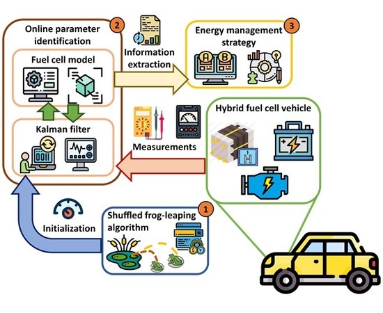
To sort out the above-discussed concerns and avoid the complex modeling of a PEMFC that demands a lot of time and experimental burdens, a third line of papers has emerged for an EMS design [20]. The idea behind this remedy is to work with data-driven (semiempirical) models—which are simpler—and to update in real time their parameters during the system operation. The whole process is performed as the PEMFC is under operation in the vehicle. This framework for upgrading the EMSs is composed of three stages, namely online parameter estimation, information extraction, and EMS. The purpose is to update the model while respecting the state variation of the PEMFC using an online identification technique, and then extract the required characteristics in the following stage. Finally, the determined operational characteristics can be utilized in the power distribution stage to control the power flow between the sources. This framework is shown in Figure 2 and can be utilized as a foundation to enhance the efficiency of the existing EMSs in an HFCV application. In [21,22,23], a Kalman filter (KF) is utilized to update the characteristics of the PEMFC stack using a semiempirical model proposed by Amphlett et al. [24,25]. This online model is then employed for different purposes in these papers. In [21], it is used to tune the output membership function of a FLC to make it insensitive against the PEMFC performance drifts. In [22], it is responsible for regularly determining the real MP and ME points of four PEMFC stacks in a multistack system. In [23], it is employed to upgrade the performance of two real-time EMSs, with the help of a simultaneous current and temperature control scheme introduced in [26], leading to 6.6% of hydrogen economy enhancement. In [27,28], recursive least square (RLS) is employed to estimate the parameters of a model obtained from the efficiency vs. power curve of the PEMFC system and then integrated into an EMS to define its efficient operation range. In [29], RLS is used in a similar way to track the changes in the hydrogen consumption rate of the PEMFC system. In [30], an EMS that is based on adaptive supervisory control is developed for a FC-battery bus, and RLS is employed for parameters estimation of a single-input PEMFC model. In [31], the performance of a single-input model, put forward by Squadrito et al. [32], is compared with the Amphlett et al. multi-input model, using RLS and KF. This benchmark study concludes that the multi-input model is more accurate than the single-input one, and KF marginally performs better than RLS in terms of precision. In [33], an adaptive system identification approach is proposed for finding the parameters of a PEMFC model. This method leads to exponential convergence while asymptotic stability is not assured. Furthermore, the robustness of the system can be included in the optimization problem formulation, which eases the burden for the online estimator. For instance, a robust formulation in [34] and an adaptive robust optimization in [35,36] are introduced by including some uncertainty sets. Although these approaches are robust against the uncertainty of parameters, they might prevent achieving the optimality. In [37], an criterion is utilized to reach a robust EMS in the presence of uncertainties that resulted from high frequency and unconsidered dynamics. In [38], chance-constrained optimization is utilized in the design of the EMS to embrace the uncertainties. It is indeed one of the major methodologies for dealing with problems under high level of uncertainties. Other methods such as designing an observer [39] and adaptive protection techniques [40] have also been utilized for increasing the robustness.
This paper utilizes a KF to estimate the parameters of a PEMFC model online. Unlike the above-discussed papers, special attention is paid to the initialization of the model parameters and the customization of KF variables in this work. An inappropriate initialization of the model parameters can lead to the misinterpretation of the physical phenomena. It can also increase the necessary time to obtain a high quality prediction of the targeted characteristics. Moreover, the improper customization of the process and measurement noise covariance matrices in KF can decrease the accuracy of the FC output voltage estimation. Once these matrices are disorganized, they keep being disorganized and will never be updated throughout the KF process. This disorganization can prevent the KF from having its best performance. To deal with this problem, this paper utilizes a metaheuristic optimization algorithm, namely shuffled frog-leaping algorithm (SFLA), for the initial offline tuning of the parameters. Subsequently, the parameters of the PEMFC model are updated online by the KF. None of the reviewed papers have had a parameters initialization analysis, which is required to justify the reliability of the estimation process. Therefore, this paper mainly concentrates on the online parameter estimation part of Figure 2, and as an example of information extraction, the polarization and power curves are extracted. These two parts have pivotal roles in this framework. The main function of the SFLA is to perform an accurate initialization for the online parameter estimator, which is responsible for updating the PEMFC model. The integration of an EMS to this framework is out of the scope of this work and can be considered in future studies. Another worth noting aspect of this work is that it has experimental validation using a 500-W PEMFC stack, as opposed to several existing papers in this domain that are merely based on simulation.
2. PEMFC Modeling
One of the most common approaches for characterizing the performance of a PEMFC stack is the use of a polarization curve, which is the plot of the stack voltage versus current (or current density) under certain conditions [41,42]. An ideal polarization curve comprises the standard reversible potential and three main losses: activation, ohmic, and concentration [41]. Activation loss appears in the low current zone mainly because of the slow kinetics of the oxygen reduction reaction. Ohmic loss takes place at the intermediate current zone primarily due to the resistance to the flow of ions in the electrolyte and the flow of electrons throughout the electrode. The concentration loss (mass transport effect) is at a high current zone owing to the limitation of the reactant gas transport through the gas diffusion layers and electrocatalyst layers.
The PEMFC model put forward by Amphlett et al. is used for the purpose of this work. This model is for several cells connected in series. It has been used for estimating the characteristics of several PEMFC technologies because of its relevant semiempirical formulation [43]. However, a new parameterization is evidently required to fit this model to the performance of different PEMFCs. The voltage of the PEMFC stack () is determined by:
where is the number of cells, is the cell voltage (V), is the reversible cell potential (V), is the activation voltage loss (V), is the ohmic voltage loss (V), and is the concentration voltage loss (V). is obtained by:
where is the temperature of the FC stack (K), is the partial pressure of hydrogen in the anode side (), and is the partial pressure of oxygen in the cathode side (). is calculated by:
where are the semiempirical parameters based on mechanistic studies, is the oxygen concentration (), and is the PEMFC operating current (A). is given by:
where is the internal resistor (. ) and are the parametric coefficients. Finally, is obtained by:
where is a parametric coefficient (V), and is the maximum current (). Since is always larger than , the natural logarithm argument is always positive. In this work, a saturation function is utilized to ensure that the natural logarithm argument remains positive in case outliers appear in the measured data.
3. Parameter Estimation
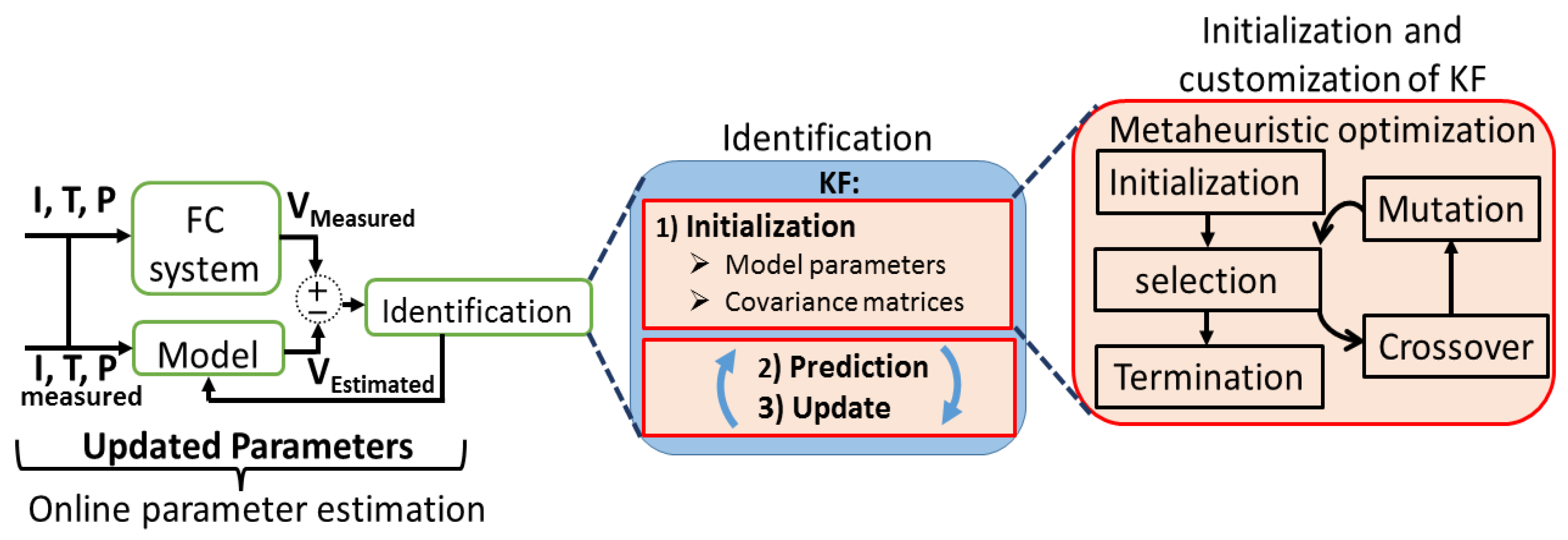
This section deals with describing the process for estimating the parametric coefficients of the previously explained PEMFC model. As mentioned earlier in Section 1, a noticeable tendency towards the online parameter estimation of PEMFC models exists in the literature. This is mainly due to the fact that a PEMFC stack undergoes some uncertainties, resulted from the degradation and variation of operating conditions, through time. When these drifts occur in the PEMFC performance, the extracted characteristics from the model are not valid until they get updated. As these characteristics, such as maximum power, are directly utilized by the EMSs, they influence the performance of a HFCV. In this respect, the online parameter estimation of a PEMFC model has attracted a lot of attention in this domain. KF is one the most well-known estimators that has been already utilized for this problem. However, the role of initialization in achieving the best performance of this process has escaped the attention of previous studies.
The details of the proposed online identification process in this paper is illustrated in Figure 3. As is seen in this figure, KF is used as the estimator to counteract the uncertainties affecting the performance of the PEMFC by tracking the model parameters online. However, before performing the online estimation, an offline initialization stage is required to determine a set of initial values for the parameters of the PEMFC model and the covariance matrices of the KF. This initialization stage is performed by means of a metaheuristic optimization algorithm, which is the most common approach for finding the parameters of a PEMFC semiempirical model offline [43]. After performing the initialization, KF is utilized for the online parameter identification purpose. It should be noted that optimal performance of KF is assumed based on having a noncorrelated distribution of each observation. Since this assumption is difficult to achieve, a careful initialization of the covariance matrices should be performed to avoid the local minimum trap or even divergence at some points.
3.1. Kalman Filter
KF is a well-known estimator for extracting the parameters of a PEMFC semiempirical model. It concludes the parameters of interest in two steps of state estimation and update as follows [44]:
where is the discrete time, is the unknown parameters vector (, , , , , , , ) obtained from (1) to (6), and denote the estimate and a priori estimate of the parameters vector, is the transition matrix taking the parameters vector from time to time , is the process noise, is the estimated output which will be the PEMFC voltage herein, is the measurement matrix (1, , , , , , ), is the measurement noise, is the error covariance matrix, is the process noise covariance matrix, is the Kalman gain, is the measurement noise covariance matrix, and is the identity matrix. is assumed to be an identity matrix because the best case scenario is that the future state will be the same as the current state, and this is exactly what an identity matrix does.
An improper initialization of the model’s unknown parameters can result in the incorrect prediction of characteristics and can increase the convergence time. This is a well-known weakness of the recursive identification techniques, which can be avoided by a proper initial tuning. Therefore, the relative certainty of the measurements and the current state estimate is an important consideration, and the main parameter that determines the weight of the predicted and measured values is the Kalman gain. It is, in fact, the gain applied to the measurements and estimation of the state and can be adjusted to attain a specific performance. When the value of the Kalman gain is high, the filter mainly trusts the new measured data and attempts to follow them rapidly. On the other hand, a low gain results in following the model predictions more closely by the filter. The Kalman gain is composed of three elements: the error covariance matrix, process noise covariance matrix, and measurement noise covariance matrix. As the initial parameters of the PEMFC model are going to be determined by special attention, the initial value of the error covariance matrix can be tuned intuitively. In fact, if one is confident about the state’s initialization, the initial error covariance matrix should be small, otherwise it should be a large value. Regarding the process noise, it indeed corresponds to the uncertainties that are expected in the state equations. The upshot of choosing a large value for the process noise is that the model is not trustworthy, and therefore the filter computes the states, but it then mostly ignores them. Concerning the measurement noise, it attempts to model the noise in the utilized sensors, which is a difficult task in practice. The common assumption is that there is no correlation in the noise among the sensors. Therefore, the variances lie on the diagonal terms, and the covariances are zero. In this paper, the explained variables are tuned by a metaheuristic optimization algorithm to avoid several heuristic trial-and-error attempts.
3.2. Shuffled Frog-Leaping Algorithm
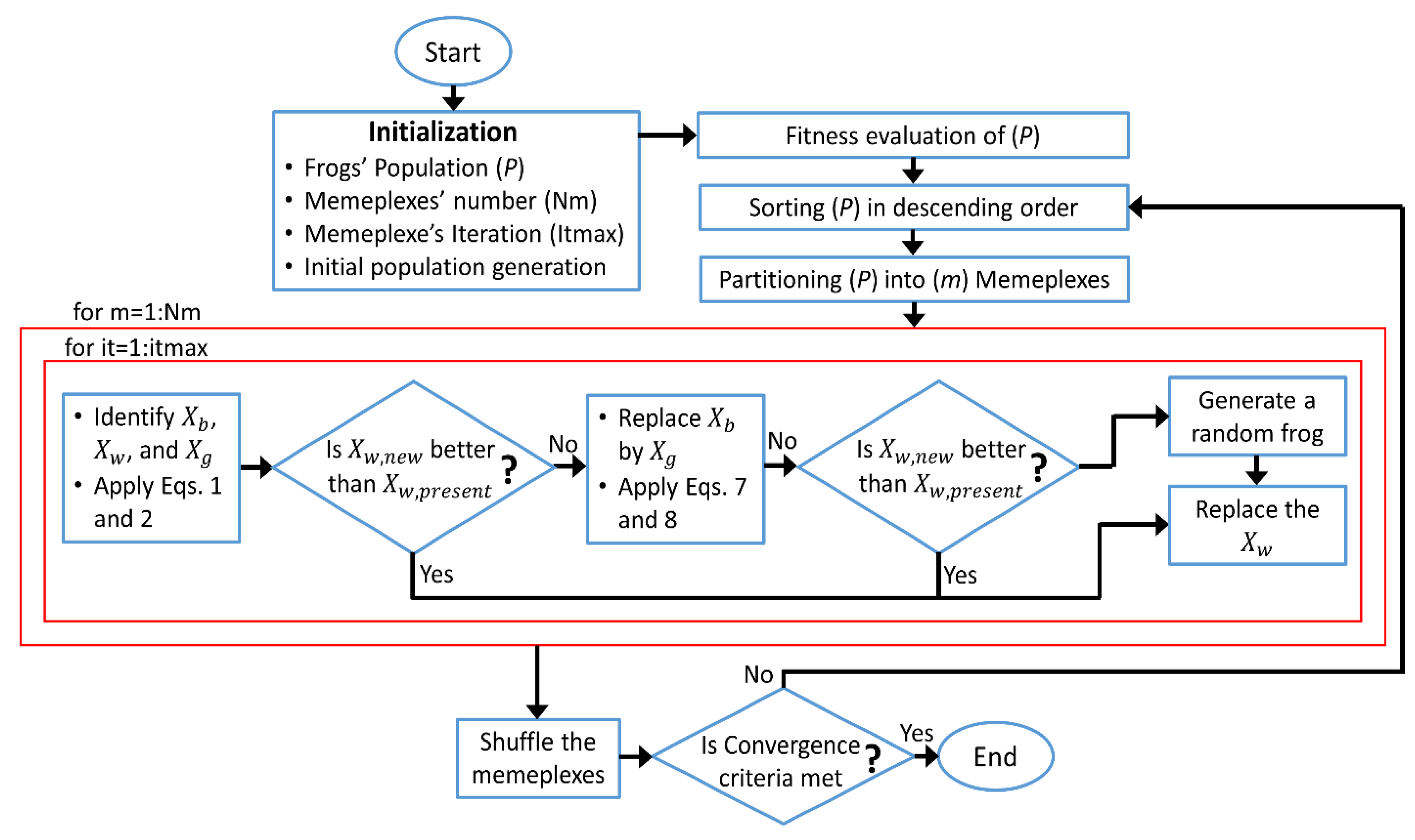
The SFLA is a memetic metaheuristic optimization method introduced in [45]. It has been used for calibrating different PEMFC models in a comparative study in [46]. A comparison of the SFLA with other competitors shows that it benefits from a satisfactory precision and reliability in a PEMFC application. This good performance primarily stems from the fact that the SFLA combines the advantages of genetic-based memetic and social behavior-based algorithms. It simultaneously performs an individual local search within each memeplex, and all the frogs are then rearranged into new memeplexes after a specific number of local iterations to assure global exploration. The flowchart of this optimization algorithm is presented in Figure 4. As is seen in this Figure, firstly, a random population () is generated in the feasible region, which is defined by the problem constraints. In a multidimensional optimization, each frog is specified by . variables as . Considering their fitness values, they are then arranged in a descending order and divided into memeplexes, each containing frogs (). The frogs are placed into the memeplexes in a particular manner. The first one is sent to the first memeplex, the second one to the second memeplex, and the th one to the th memeplex. The member is placed in the first memeplex, and this arrangement carries on up to placing all the members in all the memeplexes.
The member with the worst fitness value in each memeplex () is modified as follows:
where denotes the shift in the position, is a random number between 0 and 1, is the frog with the best answer, is the global best answer, is the new position of the worst answer, is the current position of the worst answer, and is the maximum possible variation. It is worth noting that if the worst solution does not improve with the explained formulations, (13) and (14) are recalculated by replacing with . If this modification does not enhance the solution either, it is replaced with a random solution.
So far, the optimization algorithm for the purpose of this paper has been introduced. To form an optimization problem, in addition to the algorithm, three other elements, namely an objective function, the targeted parameters for estimation, and a feasible region defined by the minimum and maximum value of each parameter, are required. In fact, the algorithm employs the objective function to guide the population in the direction of better answers within the feasible region. An evaluation criterion has an essential role in the practical application of parameter estimation methods. A proper selection of the evaluation criteria can precisely and quantitatively prove whether the techniques can obtain satisfactory outcomes. In [47], over 160 papers regarding the proton exchange membrane fuel cell parameter estimation using metaheuristic algorithms are investigated. It is then stated that the sum of squared errors (SSE) and mean squared error (MSE) are the most commonly used criteria for this problem, which have led to desirable performance. In this respect, these two metrics have been utilized in this paper.
The offline initialization has two steps. Through the first one, the initial parameters of the PEMFC model are tuned by using the polarization data of the PEMFC. The SSE of the PEMFC voltage, which shows deviations from the actual measured data, is used as the objective function to find the initial PEMFC model parameters. The SSE is defined as:
where is the measured output voltage, is the estimated voltage by the model, and is the number of sample data.
After setting the initial parameters of the model, the optimization is performed one more time for a random load profile to tune the Q and R parameters. In this second optimization, the optimization variables are just Q and R, and the model parameters are set to their optimal values obtained in the first step. In this respect, at each iteration, the optimization algorithm (SFLA) selects two best candidates for Q and R, and then KF is run for estimating the voltage of the random profile. Then, the MSE of the voltage estimation by KF is calculated, which is the objective function of the SFLA in this step. The SFLA attempts to minimize this MSE value until the last iteration. MSE is defined as:
It should be noted that the defined objective functions are only used to indicate the degree of similarities between the model and the experimental data and there is no limitation on changing or replacing them with other metrics.
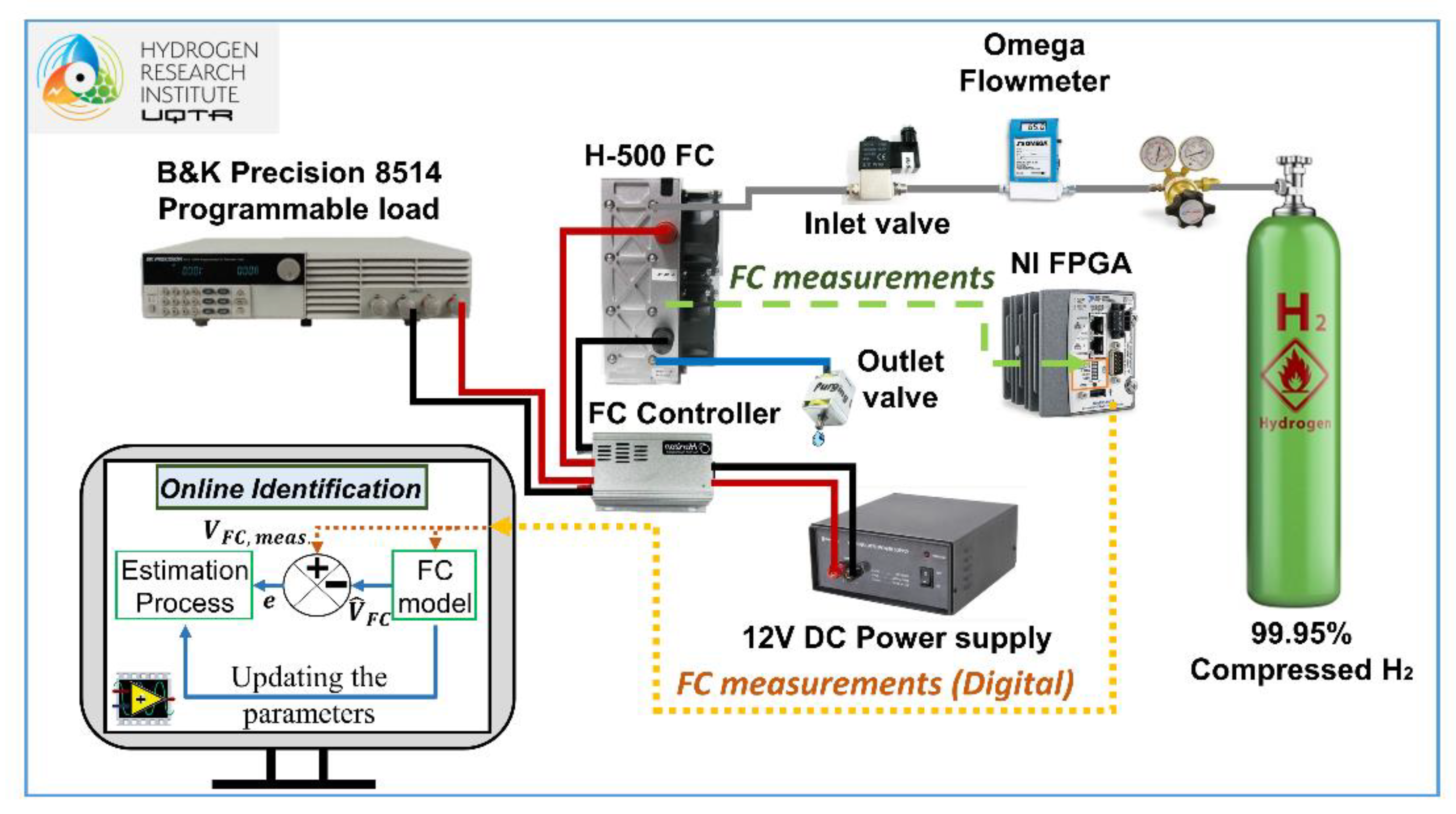
4. Experimental Setup
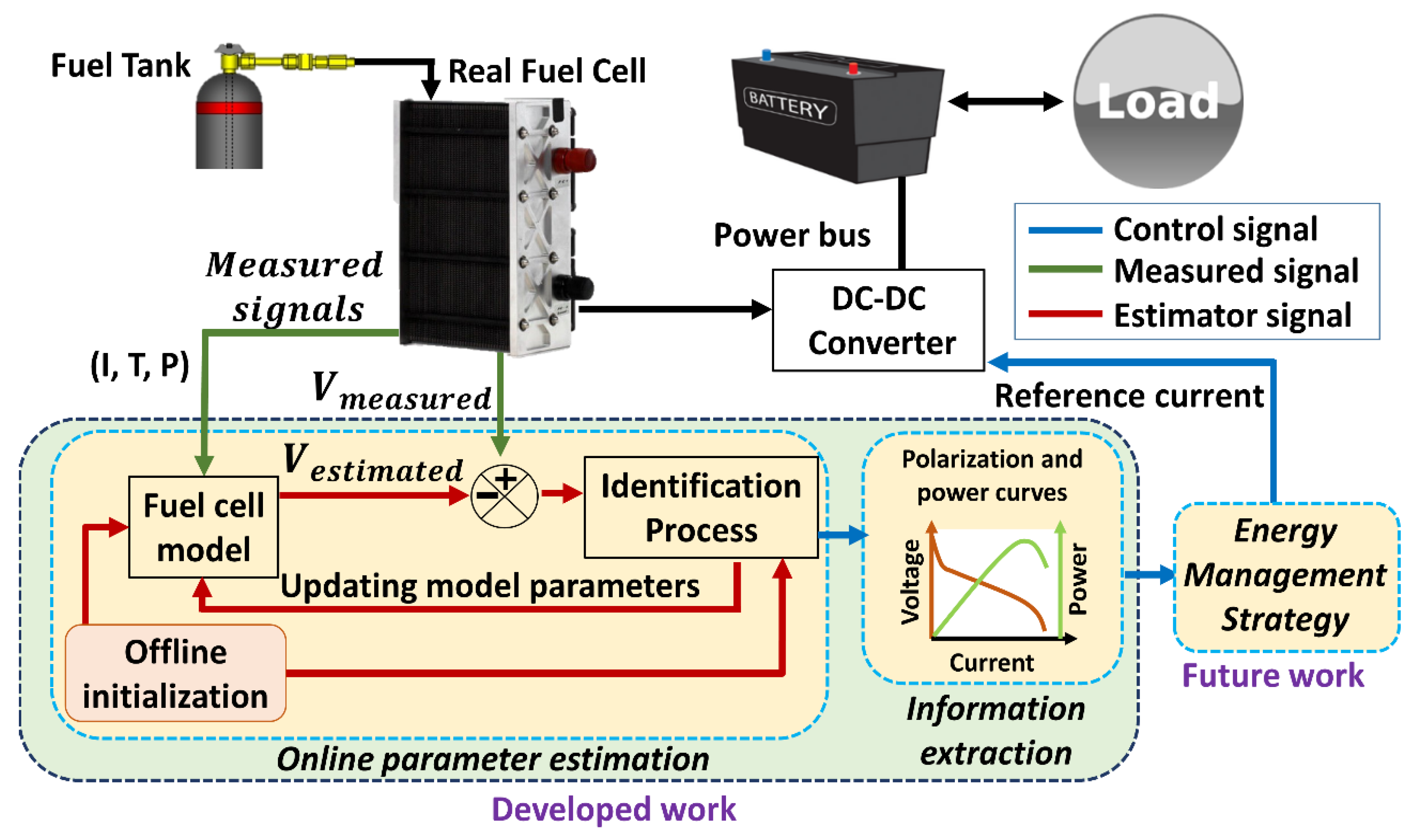
The experimental data used in this paper have been collected from a H-500 PEMFC in the hydrogen research institute of the University of Quebec in Trois-Rivieres. Figure 5 represents the employed setup for obtaining the required data. In this test bench, a 500-W Horizon PEMFC is connected to a National Instrument CompactRIO through its controller, which adjusts the stack temperature by acting on two axial fans and activates the hydrogen and the purging valves. The fans have a dual role of cooling the stack and providing the required oxygen. The other components for supplying the hydrogen include a tank, a two-stage regulator of pressure, a flowmeter, a hydrogen purging valve, and a hydrogen supply valve. According to the manufacturer, the difference between the pressure levels of the cathode and anode sides needs to be kept around 0.5 atm, which implies that the anode pressure should be set to 0.55 atm. A B&K Precision DC electronic load is utilized to demand current from the FC stack. The specifications of the utilized PEMFC, gathered from the manufacturer’s manual, are presented in Table 1. The proposed estimation process of this work is composed of two steps: offline initialization (SFLA) and online parameters estimation (KF). Regarding the offline initialization of the parameters of the PEMFC model and covariance matrices of KF, first, the required tests (applying a step-up load current profile for extracting the polarization curve and a random profile for tuning KF) are conducted on the PEMFC stack, and the corresponding measured data (current, voltage, and temperature) are recorded. It should be reminded that the partial hydrogen pressure is constant, as advised by the manufacturer. Subsequently, the measured data are used for performing the offline optimization using MATLAB software which is available in the computer. Concerning the online parameters estimation with KF, it is first developed in the MATLAB software and then implemented in the LabVIEW software, which is installed in the computer. To do so, the MathScript RT module of LabVIEW is utilized to deploy the textual math codes of MATLAB Script within LabVIEW. Therefore, in case of KF, as the measured data are received in each time step (100 ms), the estimation is performed.
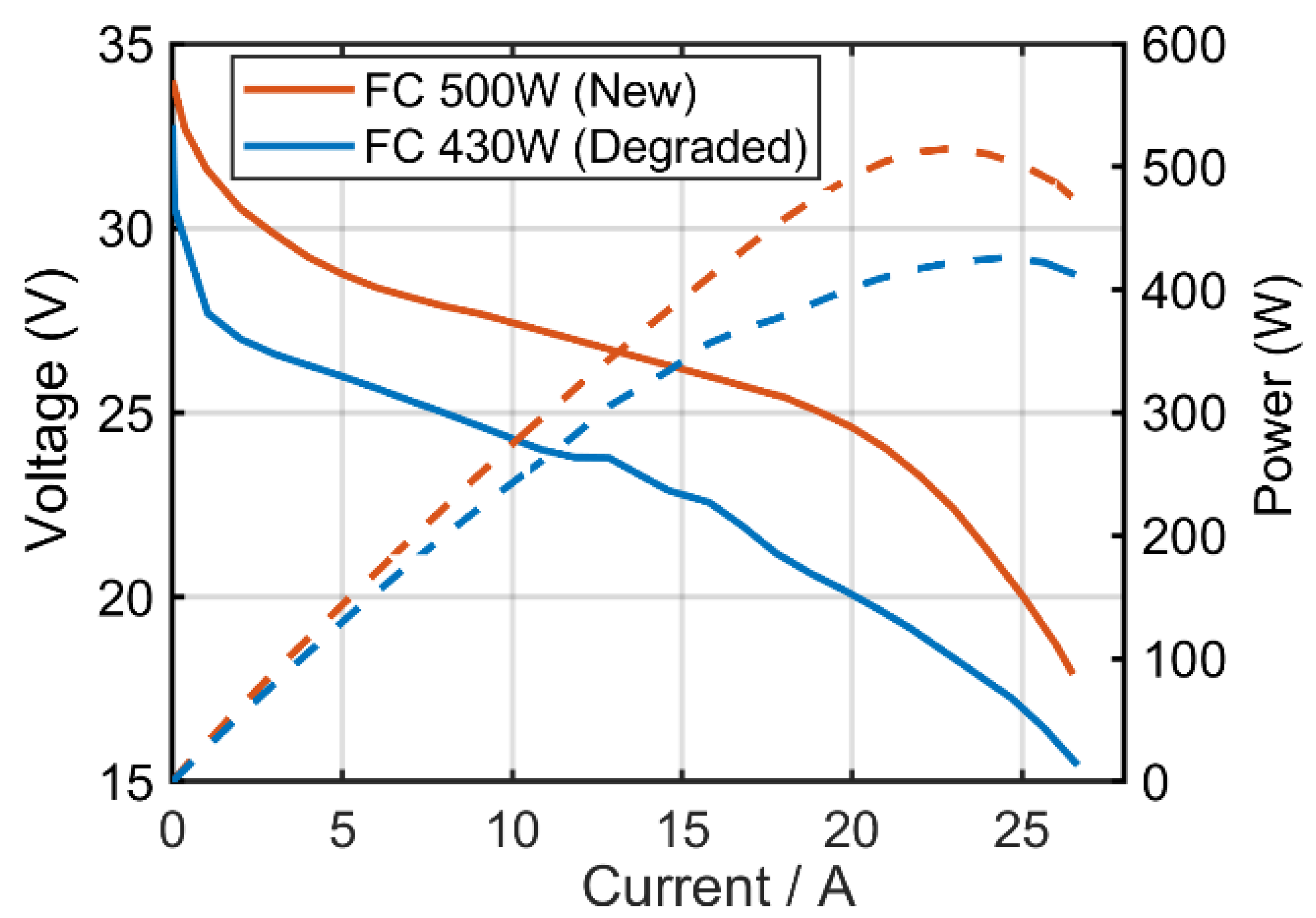
To show the present health state of the installed PEMFC on the test bench, a polarization test was conducted by pulling a constant current from the stack and measuring its corresponding voltage. The requested current is slowly increased, and the stable voltage response is recorded afterwards. After each increase in the current level, 15 to 25 min have been given to the stack to reach equilibrium. Figure 6 presents the polarization and power curves obtained from this test. Moreover, it shows the characteristics of a brand new 500-W PEMFC, extracted from the manual of the device, to clarify the occurred drifts in the employed PEMFC. As is presented in Figure 6, the maximum power of the used FC stack is 430 W, and its maximum current is 31 A. In fact, this FC has gone under degradation throughout time, and its maximum power has been reduced. The presented curves in Figure 6 are used for extracting two initialization sets to test the online identification process.
5. Discussion of the Results
To show the effectiveness of the proposed tuning process for an online parameters estimation of a PEMFC stack, some simulations based on the experimental data are performed and explained in this section. In this respect, first, the results regarding the offline initialization by the SFLA are presented and discussed. Subsequently, the effect of the initialization on the online estimator performance, which is KF, is investigated.
5.1. Offline Initialization
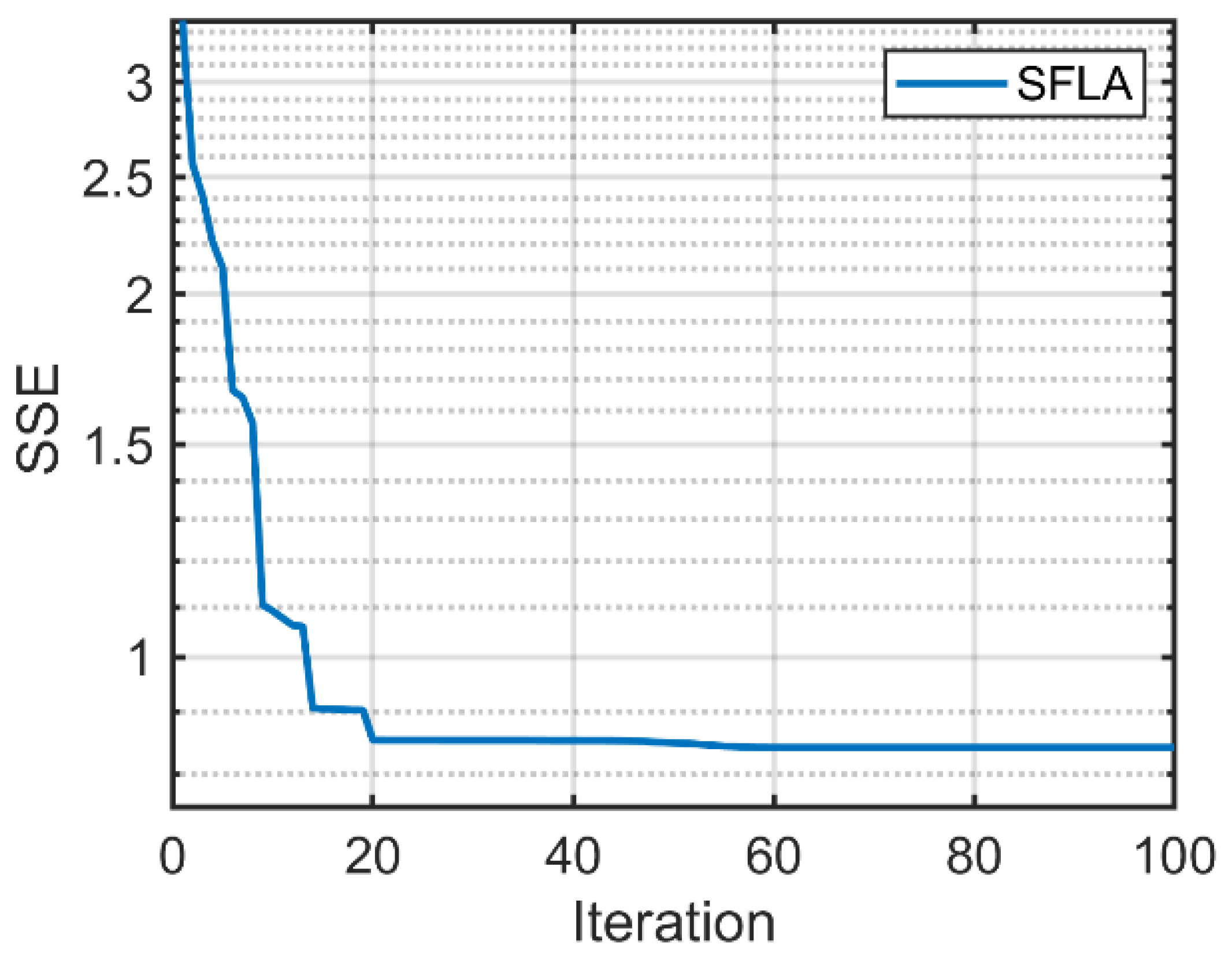
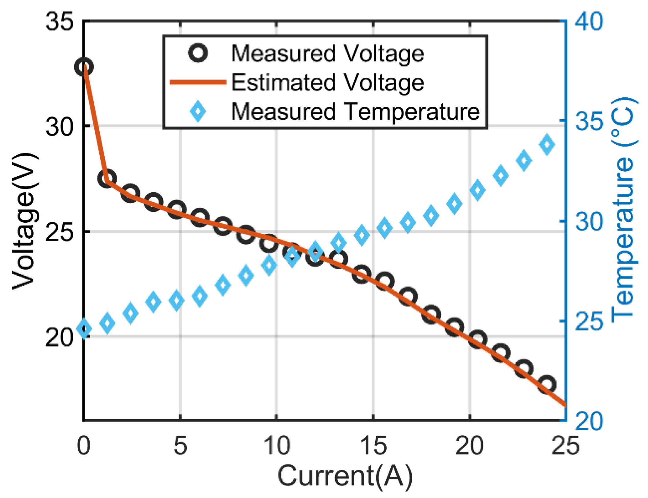
The offline optimization process with the SFLA was performed three times. First, it was done to calibrate the parameters of the PEMFC model (, , , , , , , ) for the experimental polarization curve of the installed PEMFC on the test bench using (15). Figure 7 presents the minimization trend of the SSE objective function for finding the right values of the model parameters. As is seen in this figure, the objective function value levels off almost after 50 iterations. Figure 8 shows the obtained polarization curve that resulted from the minimization of the SSE. The estimated polarization curve achieved a good precision, as quantified in the caption of Figure 8 (SSE: 0.8546). It is important to note that the value of this error is obtained by the sum of squared differences between the observed voltage and the estimated one.
After finding the initial values for the PEMFC model parameters, the optimization was performed for the second time to determine the suitable values for the covariance matrices of the KF. Figure 9 represents the minimization trend of the MSE objective function for finding the right values for Q and R matrices. As is observed, the MSE value has decreased from almost 5.79 × 10⁻⁵ to 4.32 × 10⁻⁵. Although this value is small, it approximately represents 25% of decrease in the obtained MSE, comparing the case where R and Q are assumed as 1 with the optimized ones (Q: 0.00536 and R: 84.38112). In this paper, R and Q are tuned by a metaheuristic optimization algorithm to avoid several heuristic trial-and-error attempts. In this regard, a wide range from 1e−15 to 100 was considered for these values so that the optimization algorithm can explore and find the most suitable range. According to the obtained values after the second optimization for R (84.38112) and Q (0.00536), it is realized that a small value is selected for Q and a large value is selected for R. This combination would lead to a small Kalman gain, which implies that the filter trusts the model prediction. The third optimization process was conducted to find a set of parameters for the polarization curve of the FC-500 (new FC with polarization curve from the datasheet) presented in Figure 6. This set of parameters will be utilized as an inaccurate initialization to study its influence over the online estimation in the next section. The minimization trend of this last optimization is not shown to avoid the repetition of the results. The parameters obtained through the three described optimization processes are listed in Table 2 along with the imposed inequality constraints.
5.2. Online Estimation
To inspect the effect of parameters calibration on the performance of the online estimator, two case studies are taken into consideration in this section. In the first case study, the online characteristics estimation was performed using the obtained initial parameters from the installed PEMFC on the test bench (first optimization process explained in the previous section). This set of parameters is called the optimal initialization herein. In the second case study, the online characteristics estimation is done by using the initial parameters obtained from the polarization curve of a brand new 500-W PEMFC available in the datasheet (third optimization process explained in the previous section). This set of parameters is referred to as the datasheet initialization. It is worth noting that in both described case studies, the covariance matrices of the KF are the same and are set based on the second optimization process of the preceding section.
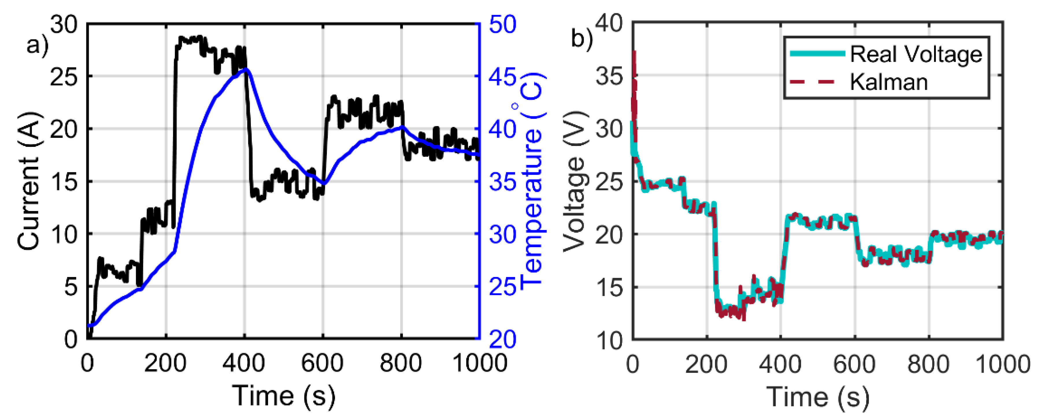
Figure 10a illustrates the current profile imposed on the installed FC in the setup and its corresponding variation of temperature. This profile is used to verify the performance of the KF in online parameters extraction of the described semiempirical model. Figure 10b compares the estimated voltage online by the KF with the measured voltage of the PEMFC. It should be noted that voltage estimation is accurate with both of initialization sets since KF attempts to minimize one single measured point at each step no matter how it changes the parameters of the model. However, it is necessary to check whether this estimation is valid during the whole operating current range of the stack. To do so, comparing the estimated polarization and power curves is very useful.
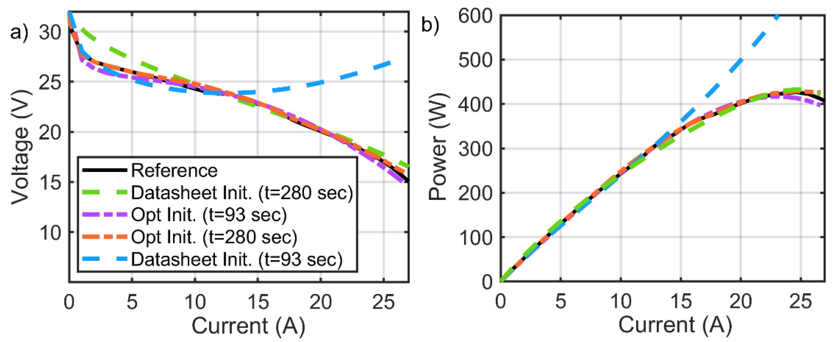
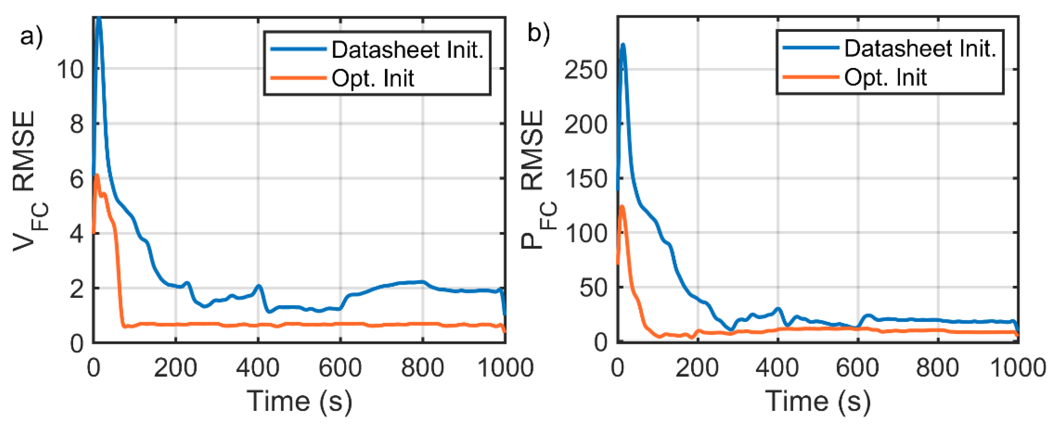
Figure 11 presents the estimated polarization (Figure 11a) and power (Figure 11b) curves of the PEMFC for two cases of optimal and datasheet initializations. From this figure, at 93 s, the estimated characteristics by using optimal initialization are more accurate than the ones obtained from the datasheet initialization set specifically in ohmic and concentration zones. On the other hand, estimating the characteristics at 280 s shows that the quality of estimation by using the datasheet initialization set can be improved by giving more time to the estimator. These results imply that a precise characteristics estimation can be achieved in less time and more conveniently when starting the estimation process with the appropriate initialization. This can also be very interesting in applications where the fast prediction of the maximum power is needed, such as the PEMFC cold start-up. Figure 12 shows the variation of the root MSE (RMSE) for each of the considered case studies using the datasheet and optimal initial conditions. Figure 12a shows the RMSE trend for the polarization curve, and Figure 12b illustrates the RMSE convergence trend for the power curve. Comparing the obtained RMSE values in both the polarization and power curves in this figure shows that the optimal initialization can lead to achieving more accuracy in a shorter time.
6. Conclusions
This paper proposes a framework that can be used as a basis to enhance the efficiency and reliability of the existing EMSs for HFCVs. The core of the proposed framework is an online parameter estimation method based on the KF, with special attention to the initialization and customization stages of this filter, to update the parameters of a PEMFC model while the vehicle is running. The updated model can be used to feed the EMS with realistic operational characteristics. Herein, the initialization of KF is performed in two steps by using SFLA metaheuristic optimization algorithm. The first step deals with finding the right primary values for the targeted PEMFC model parameters, and the second step copes with tuning the values of R and Q covariance matrices of the KF. After finding the appropriate initialization values for different variables, the KF is used online to extract the right parameters for the PEMFC stack. The final results of this work confirm that a good initialization can improve the estimation quality in terms of speed and precision. In fact, finding the appropriate initial values for the PEMFC model parameters of interest leads to estimating better characteristics curves in a shorter time, and the tuning of the covariance matrices enhances the estimation accuracy to a certain level.
The results of this work have created some opportunities for extending the scope of this paper as follows:
- The focus of this work is mainly on the parameter extraction in ambient temperature. However, the outcomes seem to be very interesting in applications where a fast performant identification is required. In this regard, future works should focus on the utilization of such strategy for performing the adaptive cold start-up of the PEMFC stack.
- This paper has discussed the use of the KF with a specific view to proper initialization for estimating the parameters of a PEMFC model online. Afterwards, as an example, the updated model was utilized for determining the maximum power of the PEMFC stack at each moment (first and second steps of the proposed framework). The future works can use the provided basis in this article to design different online EMSs for a HFCV.
Abbreviations:
| ECMS | Equivalent consumption minimization strategy |
| EMS | Energy management strategy |
| ESA | Extremum seeking algorithm |
| FC | Fuel cell |
| FLCs | Fuzzy logic controllers |
| HFCV | Hybrid fuel cell vehicle |
| KF | Kalman filter |
| ME | Maximum efficiency |
| MP | Maximum power |
| MSE | Mean squared error |
| PEMFC | Proton exchange membrane fuel cell |
| RLS | Recursive least square |
| RMSE | Root mean squared error |
| SC | Supercapacitor |
| SFLA | Shuffled frog-leaping algorithm |
| SOC | State of charge |
| SSE | Sum of squared errors |
Author Contributions
Conceptualization, M.K.; formal analysis, L.B. and J.P.F.T.; funding acquisition, M.K., L.B. and J.P.F.T.; methodology, M.K. and A.M.; software, M.K. and A.M.; supervision, L.B. and J.P.F.T.; writing—original draft, M.K.; writing—review and editing, M.K., A.M., L.B., and J.P.F.T. All authors have read and agreed to the published version of the manuscript.
Funding
This research was funded by Fonds de Recherche du Québec–Nature et technologies (FRQNT) [Bourses de recherche postdoctorale B3X, file number: 284914], Natural Sciences and Engineering Research Council of Canada (NSERC) [RGPIN-2018-06527 and RGPIN-2017-05924], and Canada Research Chairs program [950-230863 and 950-230672].
Conflicts of Interest
The authors declare no conflict of interest. The funders had no role in the design of the study; in the collection, analyses, or interpretation of data; in the writing of the manuscript; or in the decision to publish the results.
References
- Bartecka, M.; Barchi, G.; Paska, J.A. Time-Series PV Hosting Capacity Assessment with Storage Deployment. Energies 2020, 13, 2524. [Google Scholar] [CrossRef]
- Qamar, S.Z.; Al-Kindi, M. Renewability and Sustainability: Current Status and Future Prospects. In Encyclopedia of Renewable and Sustainable Materials; Hashmi, S., Choudhury, I.A., Eds.; Elsevier: Oxford, UK, 2020; pp. 717–730. [Google Scholar] [CrossRef]
- Karamanev, D.; Pupkevich, V.; Penev, K.; Glibin, V.; Gohil, J.; Vajihinejad, V. Biological conversion of hydrogen to electricity for energy storage. Energy 2017, 129, 237–245. [Google Scholar] [CrossRef]
- Manoharan, Y.; Hosseini, E.S.; Butler, B.; Alzhahrani, H.; Senior, T.B.; Ashuri, T.; Krohn, J. Hydrogen Fuel Cell Vehicles; Current Status and Future Prospect. Appl. Sci. 2019, 9, 2296. [Google Scholar] [CrossRef] [Green Version]
- Wilberforce, T.; Alaswad, A.; Palumbo, A.; Dassisti, M.; Olabi, A.G. Advances in stationary and portable fuel cell applications. Int. J. Hydrog. Energy 2016, 41, 16509–16522. [Google Scholar] [CrossRef] [Green Version]
- GM, US Navy partner on fuel cell powered underwater vehicles. Fuel Cells Bull. 2016, 2016, 4. [CrossRef]
- González Palencia, C.J.; Nguyen, T.V.; Araki, M.; Shiga, S. The Role of Powertrain Electrification in Achieving Deep Decarbonization in Road Freight Transport. Energies 2020, 13, 2459. [Google Scholar] [CrossRef]
- Gherairi, S. Hybrid Electric Vehicle: Design and Control of a Hybrid System (Fuel Cell/Battery/Ultra-Capacitor) Supplied by Hydrogen. Energies 2019, 12, 1272. [Google Scholar] [CrossRef] [Green Version]
- Kandi Dayeni, M.; Soleymani, M. Intelligent energy management of a fuel cell vehicle based on traffic condition recognition. Clean Technol. Environ. Policy 2016, 18, 1945–1960. [Google Scholar] [CrossRef]
- Ali, M.A.; Söffker, D. Towards Optimal Power Management of Hybrid Electric Vehicles in Real-Time: A Review on Methods, Challenges, and State-of-the-Art Solutions. Energies 2018, 11, 476. [Google Scholar] [CrossRef] [Green Version]
- Sulaiman, N.; Hannan, M.A.; Mohamed, A.; Ker, P.J.; Majlan, E.H.; Wan Daud, W.R. Optimization of energy management system for fuel-cell hybrid electric vehicles: Issues and recommendations. Appl. Energy 2018, 228, 2061–2079. [Google Scholar] [CrossRef]
- Zheng, Y.; He, F.; Shen, X.; Jiang, X. Energy Control Strategy of Fuel Cell Hybrid Electric Vehicle Based on Working Conditions Identification by Least Square Support Vector Machine. Energies 2020, 13, 426. [Google Scholar] [CrossRef] [Green Version]
- Chen, X.; Hu, G.; Guo, F.; Ye, M.; Huang, J. Switched Energy Management Strategy for Fuel Cell Hybrid Vehicle Based on Switch Network. Energies 2020, 13, 247. [Google Scholar] [CrossRef] [Green Version]
- Snoussi, J.; Ben Elghali, S.; Benbouzid, M.; Mimouni, F.M. Auto-Adaptive Filtering-Based Energy Management Strategy for Fuel Cell Hybrid Electric Vehicles. Energies 2018, 11, 2118. [Google Scholar] [CrossRef] [Green Version]
- Ettihir, K.; Boulon, L.; Agbossou, K. Energy management strategy for a fuel cell hybrid vehicle based on maximum efficiency and maximum power identification. IET Electr. Syst. Transp. 2016, 6, 261–268. [Google Scholar] [CrossRef]
- Wang, Y.; Moura, S.J.; Advani, S.G.; Prasad, A.K. Power management system for a fuel cell/battery hybrid vehicle incorporating fuel cell and battery degradation. Int. J. Hydrog. Energy 2019, 44, 8479–8492. [Google Scholar] [CrossRef]
- Li, H.; Ravey, A.; N’Diaye, A.; Djerdir, A. Online adaptive equivalent consumption minimization strategy for fuel cell hybrid electric vehicle considering power sources degradation. Energy Convers. Manag. 2019, 192, 133–149. [Google Scholar] [CrossRef]
- Zhou, D.; Al-Durra, A.; Matraji, I.; Ravey, A.; Gao, F. Online Energy Management Strategy of Fuel Cell Hybrid Electric Vehicles: A Fractional-Order Extremum Seeking Method. IEEE Trans. Ind. Electron. 2018, 65, 6787–6799. [Google Scholar] [CrossRef]
- Bizon, N. Energy optimization of fuel cell system by using global extremum seeking algorithm. Appl. Energy 2017, 206, 458–474. [Google Scholar] [CrossRef]
- Ettihir, K.; Boulon, L.; Agbossou, K. Optimization-based energy management strategy for a fuel cell/battery hybrid power system. Appl. Energy 2016, 163, 142–153. [Google Scholar] [CrossRef]
- Kandidayeni, M.; Fernandez, A.O.M.; Khalatbarisoltani, A.; Boulon, L.; Kelouwani, S.; Chaoui, H. An Online Energy Management Strategy for a Fuel Cell/Battery Vehicle Considering the Driving Pattern and Performance Drift Impacts. IEEE Trans. Veh. Technol. 2019, 68, 11427–11438. [Google Scholar] [CrossRef]
- Fernandez, A.M.; Kandidayeni, M.; Boulon, L.; Chaoui, H. An Adaptive State Machine Based Energy Management Strategy for a Multi-Stack Fuel Cell Hybrid Electric Vehicle. IEEE Trans. Veh. Technol. 2020, 69, 220–234. [Google Scholar] [CrossRef]
- Kandidayeni, M.; Fernandez, A.M.; Boulon, L.; Kelouwani, S. Efficiency Upgrade of Hybrid Fuel Cell Vehicles’ Energy Management Strategies by Online Systemic Management of Fuel Cell. IEEE Trans. Ind. Electron. 2020. [Google Scholar] [CrossRef]
- Amphlett, J.C. Performance Modeling of the Ballard Mark IV Solid Polymer Electrolyte Fuel Cell. J. Electrochem. Soc. 1995, 142, 9. [Google Scholar] [CrossRef]
- Mann, R.F.; Amphlett, J.C.; Hooper, M.A.I.; Jensen, H.M.; Peppley, B.A.; Roberge, P.R. Development and application of a generalised steady-state electrochemical model for a PEM fuel cell. J. Power Sour. 2000, 86, 173–180. [Google Scholar] [CrossRef]
- Kandidayeni, M.F.A.M.; Boulon, L.; Kelouwani, S. Efficiency Enhancement of an Open Cathode Fuel Cell Through a Systemic Management. IEEE Trans. Veh. Technol. 2019, 68, 11462–11472. [Google Scholar] [CrossRef]
- Wang, T.; Li, Q.; Qiu, Y.; Yin, L.; Liu, L.; Chen, W. Efficiency Extreme Point Tracking Strategy Based on FFRLS Online Identification for PEMFC System. IEEE Trans. Energy Convers. 2019, 34, 952–963. [Google Scholar] [CrossRef]
- Wang, T.; Li, Q.; Wang, X.; Qiu, Y.; Liu, M.; Meng, X.; Li, J.; Chen, W. An optimized energy management strategy for fuel cell hybrid power system based on maximum efficiency range identification. J. Power Sour. 2020, 445, 227333. [Google Scholar] [CrossRef]
- Wang, T.; Li, Q.; Yin, L.; Chen, W. Hydrogen consumption minimization method based on the online identification for multi-stack PEMFCs system. Int. J. Hydrog. Energy 2019, 44, 5074–5081. [Google Scholar] [CrossRef]
- Xu, L.; Li, J.; Hua, J.; Li, X.; Ouyang, M. Adaptive supervisory control strategy of a fuel cell/battery-powered city bus. J. Power Sour. 2009, 194, 360–368. [Google Scholar] [CrossRef]
- Kandidayeni, M.; Macias, A.; Amamou, A.A.; Boulon, L.; Kelouwani, S.; Chaoui, H. Overview and benchmark analysis of fuel cell parameters estimation for energy management purposes. J. Power Sour. 2018, 380, 92–104. [Google Scholar] [CrossRef] [Green Version]
- Squadrito, G.; Maggio, G.; Passalacqua, E.; Lufrano, F.; Patti, A. An empirical equation for polymer electrolyte fuel cell (PEFC) behaviour. J. Appl. Electrochem. 1999, 29, 1449–1455. [Google Scholar] [CrossRef]
- Xing, Y.; Na, J.; Costa-Castelló, R. Real-Time Adaptive Parameter Estimation for a Polymer Electrolyte Membrane Fuel Cell. IEEE Trans. Ind. Inform. 2019, 15, 6048–6057. [Google Scholar] [CrossRef] [Green Version]
- Hosseinzadeh, M.; Salmasi, F.R. Robust Optimal Power Management System for a Hybrid AC/DC Micro-Grid. IEEE Trans. Sustain. Energy 2015, 6, 675–687. [Google Scholar] [CrossRef]
- Mohiti, M.; Monsef, H.; Anvari-moghaddam, A.; Guerrero, J.; Lesani, H. A decentralized robust model for optimal operation of distribution companies with private microgrids. Int. J. of Electr. Power Energy Syst. 2019, 106, 105–123. [Google Scholar] [CrossRef]
- Lara, J.D.; Olivares, D.E.; Cañizares, C.A. Robust Energy Management of Isolated Microgrids. IEEE Syst. J. 2019, 13, 680–691. [Google Scholar] [CrossRef]
- Hosseinalizadeh, T.; Kebriaei, H.; Salmasi, F.R. Decentralised robust T-S fuzzy controller for a parallel islanded AC microgrid. IET Gener. Transm. Distrib. 2019, 13, 1589–1598. [Google Scholar] [CrossRef]
- Javadi, M.S.; Lotfi, M.; Esmaeelnezhad, A.; Anvari-Moghaddam, A.; Guerrero, J.M.; Catalao, J. Optimal Operation of Energy Hubs Considering Uncertainties and Different Time Resolutions. IEEE Trans. Ind. Appl. 2020. [Google Scholar] [CrossRef]
- Saim, A.; Houari, A.; Guerrero, J.M.; Djerioui, A.; Machmoum, M.; Ahmed, M.A. Stability Analysis and Robust Damping of Multiresonances in Distributed-Generation-Based Islanded Microgrids. IEEE Trans. Ind. Electron. 2019, 66, 8958–8970. [Google Scholar] [CrossRef]
- Hussain, N.; Nasir, M.; Vasquez, J.C.; Guerrero, J.M. Recent Developments and Challenges on AC Microgrids Fault Detection and Protection Systems–A Review. Energies 2020, 13, 2149. [Google Scholar] [CrossRef]
- Ade, N.; Wilhite, B.; Goyette, H.; Mannan, M.S. Intensifying vehicular proton exchange membrane fuel cells for safer and durable, design and operation. Int. J. Hydrog. Energy 2020, 45, 5039–5054. [Google Scholar] [CrossRef]
- Zhong, D.; Lin, R.; Jiang, Z.; Zhu, Y.; Liu, D.; Cai, X.; Chen, L. Low temperature durability and consistency analysis of proton exchange membrane fuel cell stack based on comprehensive characterizations. Appl. Energy 2020, 264, 114626. [Google Scholar] [CrossRef]
- Priya, K.; Sathishkumar, K.; Rajasekar, N. A comprehensive review on parameter estimation techniques for Proton Exchange Membrane fuel cell modelling. Renew. Sustain. Energy Rev. 2018, 93, 121–144. [Google Scholar] [CrossRef]
- Haykin, S. Kalman Filters. In Kalman Filtering and Neural Networks; John Wiley & Sons: Hoboken, NJ, USA, 2002. [Google Scholar] [CrossRef]
- Eusuff, M.; Lansey, K.; Pasha, F. Shuffled frog-leaping algorithm: A memetic meta-heuristic for discrete optimization. Eng. Optim. 2006, 38, 129–154. [Google Scholar] [CrossRef]
- Kandidayeni, M.; Macias, A.; Khalatbarisoltani, A.; Boulon, L.; Kelouwani, S. Benchmark of proton exchange membrane fuel cell parameters extraction with metaheuristic optimization algorithms. Energy 2019, 183, 912–925. [Google Scholar] [CrossRef]
- Yang, B.; Wang, J.; Yu, L.; Shu, H.; Yu, T.; Zhang, X.; Yao, W.; Sun, L. A critical survey on proton exchange membrane fuel cell parameter estimation using meta-heuristic algorithms. J. Clean. Prod. 2020, 265, 121660. [Google Scholar] [CrossRef]
Figure 1.
Application of a proton exchange membrane fuel cell (PEMFC) in different domains.

Figure 2.
The proposed framework to upgrade the efficiency of an energy management strategy (EMS).

Figure 3.
The online fuel cell (FC) parameters estimation along with the initialization process.

Figure 4.
The flowchart of shuffled frog-leaping algorithm (SFLA) [46].
Figure 4.
The flowchart of shuffled frog-leaping algorithm (SFLA) [46].

Figure 5.
The utilized experimental setup.

Figure 6.
The comparison of the utilized PEMFC characteristics with a brand new one.

Figure 7.
The convergence graph of the defined sum of squared errors (SSE).

Figure 8.
The obtained polarization curve using SFLA (SSE: 0.8546).

Figure 9.
The mean squared error (MSE) objective function minimization trend for finding the optimized values (Q: 0.00536 and R: 84.38112).
Figure 9.
The mean squared error (MSE) objective function minimization trend for finding the optimized values (Q: 0.00536 and R: 84.38112).

Figure 10.
Estimation of the voltage of the real PEMFC. (a) Current profile and stack temperature variation; (b) voltage estimation by the Kalman filter (KF).
Figure 10.
Estimation of the voltage of the real PEMFC. (a) Current profile and stack temperature variation; (b) voltage estimation by the Kalman filter (KF).

Figure 11.
Characteristics estimation: (a) polarization curve estimation; (b) power curve estimation.
Figure 11.
Characteristics estimation: (a) polarization curve estimation; (b) power curve estimation.

Figure 12.
Variation of root MSE (RMSE) estimation: (a) polarization curve; (b) power curve.


Table 1.
The specifications of an H-500 open cathode FC.
| Technical Specifications | |
|---|---|
| FC type | PEM |
| Rated power | 500 W |
| Rated performance | 22 V @ 23.5 A |
| Max current | 35 A |
| Rated H2 consumption | 7 SLPM |
| Ambient temperature | 5 to 30 |
| Max stack temperature | 65 |
| Cooling | Air (integrated cooling fan) |
| Reactants | Hydrogen and air |
| Number of cells | 36 |
Table 2.
The obtained parameters after the optimization processes.
| Optimization Process | Obtained Value | Minimum Value | Maximum Value |
|---|---|---|---|
| First | = −1.167 | −1.2 | −0.80 |
| = 1.00 × 10⁻³ | 1 × 10⁻³ | 5 × 10⁻³ | |
| = 9.83 × 10⁻⁵ | 3.6 × 10⁻³ | 9.8 × 10⁻³ | |
| = −1.102 × 10⁻⁴ | −2.6 × 10⁻⁴ | −0.954 × 10⁻⁴ | |
| 0.16 | 0.22 | ||
| = 0.174 | 0.0135 | 0.5 | |
| Second | = 0.00536 | 1 × 10⁻¹⁵ | 100 |
| = 84.38112 | 1 × 10⁻¹⁵ | 100 | |
| Third | = −0.973 | −1.2 | −0.80 |
| = 1.533 × 10⁻³ | 1 × 10⁻³ | 5 × 10⁻³ | |
| = 3.6451 × 10⁻⁵ | 3.6 × 10⁻³ | 9.8 × 10⁻³ | |
| = −9.540 × 10⁻⁵ | −2.6 × 10⁻⁴ | −0.954 × 10⁻⁴ | |
| 0.16 | 0.22 | ||
| = 0.0136 | 0.0135 | 0.5 |
© 2020 by the authors. Licensee MDPI, Basel, Switzerland. This article is an open access article distributed under the terms and conditions of the Creative Commons Attribution (CC BY) license (http://creativecommons.org/licenses/by/4.0/).
Share and Cite
MDPI and ACS Style
Kandidayeni, M.; Macias, A.; Boulon, L.; Trovão, J.P.F. Online Modeling of a Fuel Cell System for an Energy Management Strategy Design. Energies 2020, 13, 3713. https://0-doi-org.brum.beds.ac.uk/10.3390/en13143713
AMA Style
Kandidayeni M, Macias A, Boulon L, Trovão JPF. Online Modeling of a Fuel Cell System for an Energy Management Strategy Design. Energies. 2020; 13(14):3713. https://0-doi-org.brum.beds.ac.uk/10.3390/en13143713
Chicago/Turabian StyleKandidayeni, Mohsen, Alvaro Macias, Loïc Boulon, and João Pedro F. Trovão. 2020. "Online Modeling of a Fuel Cell System for an Energy Management Strategy Design" Energies 13, no. 14: 3713. https://0-doi-org.brum.beds.ac.uk/10.3390/en13143713
Note that from the first issue of 2016, this journal uses article numbers instead of page numbers. See further details here.