Article

Application of the 2-D Trefftz Method for Identification of Flow Boiling Heat Transfer Coefficient in a Rectangular MiniChannel

by
Mirosław Grabowski
1,*,
Sylwia Hożejowska
2,
Beata Maciejewska
2,
Krzysztof Płaczkowski
1 and
Mieczysław E. Poniewski
1
1
Faculty of Civil Engineering, Mechanics and Petrochemistry, Warsaw University of Technology, 09-400 Płock, Poland
2
Faculty of Management and Computer Modelling, Kielce University of Technology, 25-314 Kielce, Poland
*
Author to whom correspondence should be addressed.
Submission received: 25 May 2020 / Revised: 13 July 2020 / Accepted: 21 July 2020 / Published: 2 August 2020
(This article belongs to the Special Issue Thermal Systems)

Abstract

:
The study presents the experimental and numeric heat transfer investigations in flow boiling of water through an asymmetrically heated, rectangular and horizontal minichannel, with transparent side walls. A dedicated system was designed to record images of two-phase flow structures using a high-speed video camera with a synchronous movement system. The images were analyzed with Matlab 2019a scripts for determination of the void fraction for each pattern of two-phase flow structures observed. The experimental data measured during the experimental runs included inlet and outlet temperature, temperature at three internal points of the heater body, volume flux of the flowing water, inlet pressure, pressure drop, current and the voltage drop in the heater power supply. The flows were investigated at Reynolds number characteristic of laminar flow. The mathematical model assumed the heat transfer process in the measurement module to be steady-state with temperature independent thermal properties of solids and flowing fluid. The defined two inverse heat transfer problems were solved with the Trefftz method with two sets of T- functions. Graphs were used to represent: the boiling curves, the local void fraction values, the boiling heat transfer coefficients and the errors of both of them for selected mass fluxes and heat fluxes.

Graphical Abstract

1. Introduction

A growing necessity of transferring very high heat fluxes from both miniaturized industrial equipment and home appliances generates demand for mini- or micro-scale cooling devices. Some cooling systems require low pumping power and consequently low Reynolds numbers for the flow [1,2,3]. In such cases, flow boiling heat transfer, which is characteristic of high heat transfer coefficients, appears to be the appropriate solution. The determination of the heat transfer coefficient requires knowledge of the parameters of the boiling fluid flowing in the minichannel. These parameters are in particular: temperature and pressure at characteristic points of the system, mass flux of the boiling fluid, heat flux and void fraction. The measurements of the void fraction were combined with photographic recording of boiling two-phase flow structures, characteristic for horizontal orientation of the minichannel [4,5].
The obtained experimental data for water flow boiling in a single rectangular minichannel at a low Reynolds number provided the basis for numeric analysis with the use of Trefftz method [6]. Direct heat conduction problems—DHCPs—Appear in mathematical modeling of steady-state heat transfer problems when the governing equation, domain, boundary conditions and physical properties of the material are known. When any of these elements is unknown, we must deal with an inverse heat conduction problem—IHCP. High sensitivity to uncertainty of incoming data are a characteristic feature of many engineering inverse problems. This weakness can get enhanced when two or three succeeding inverse problems are taken into account. Therefore, solving inverse problems requires efficient and stable numeric methods. As the Trefftz method with a set of T-functions fulfills this requirement [7,8,9,10,11], it was used to solve the IHCP problem for flow boiling in the minichannel. Two sets of T-functions were applied to calculate: (a) two-dimensional temperature distributions of the heating copper block and the boiling water, (b) heating copper block temperature gradients, and (c) the heat transfer coefficient at the contact surface copper block–flowing fluid.

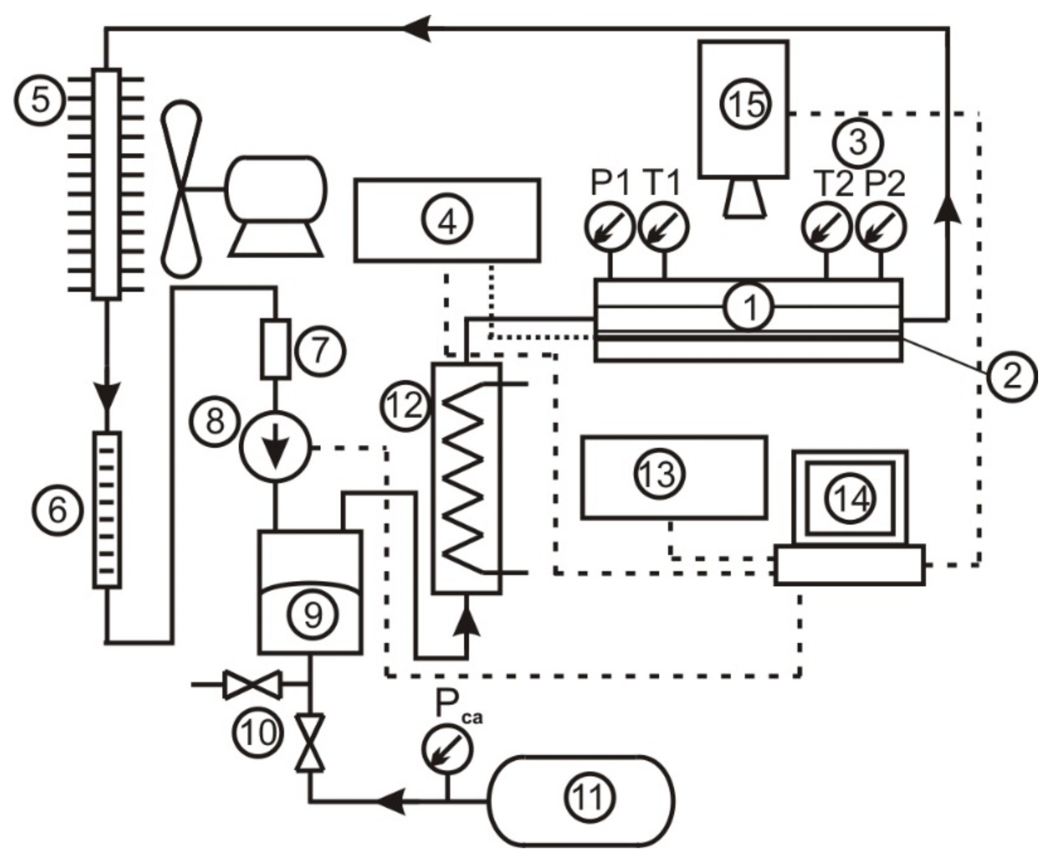
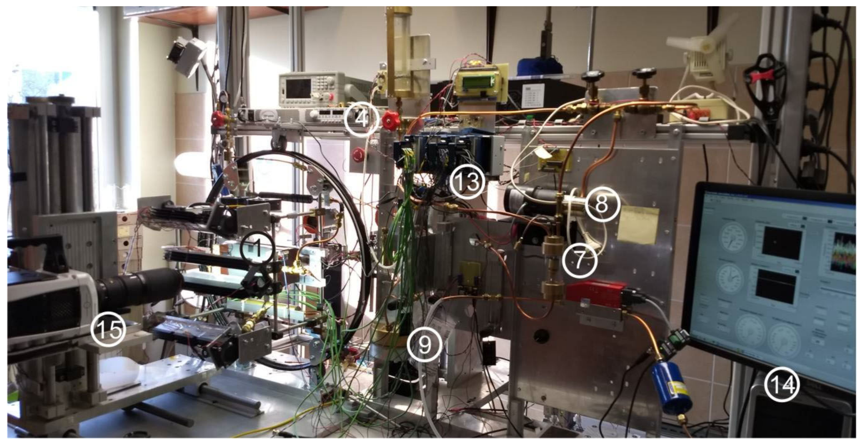
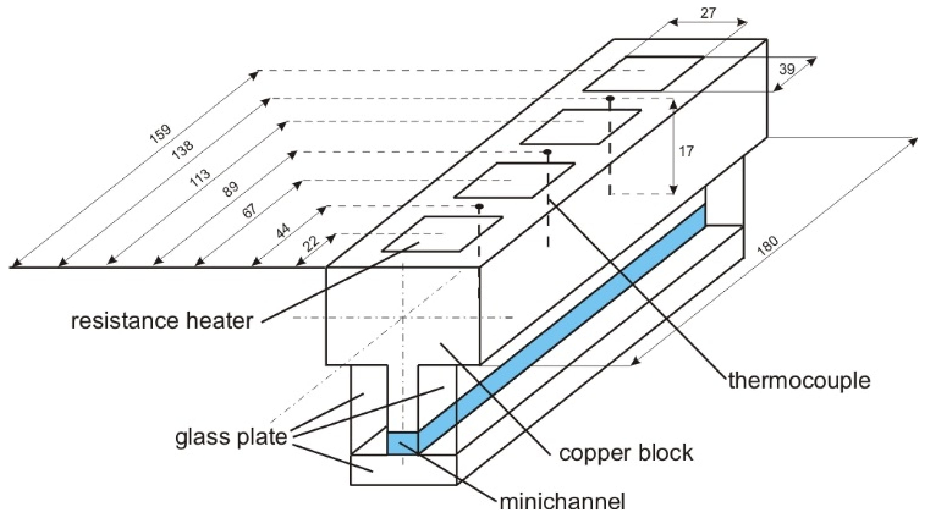
2. Experimental Facility

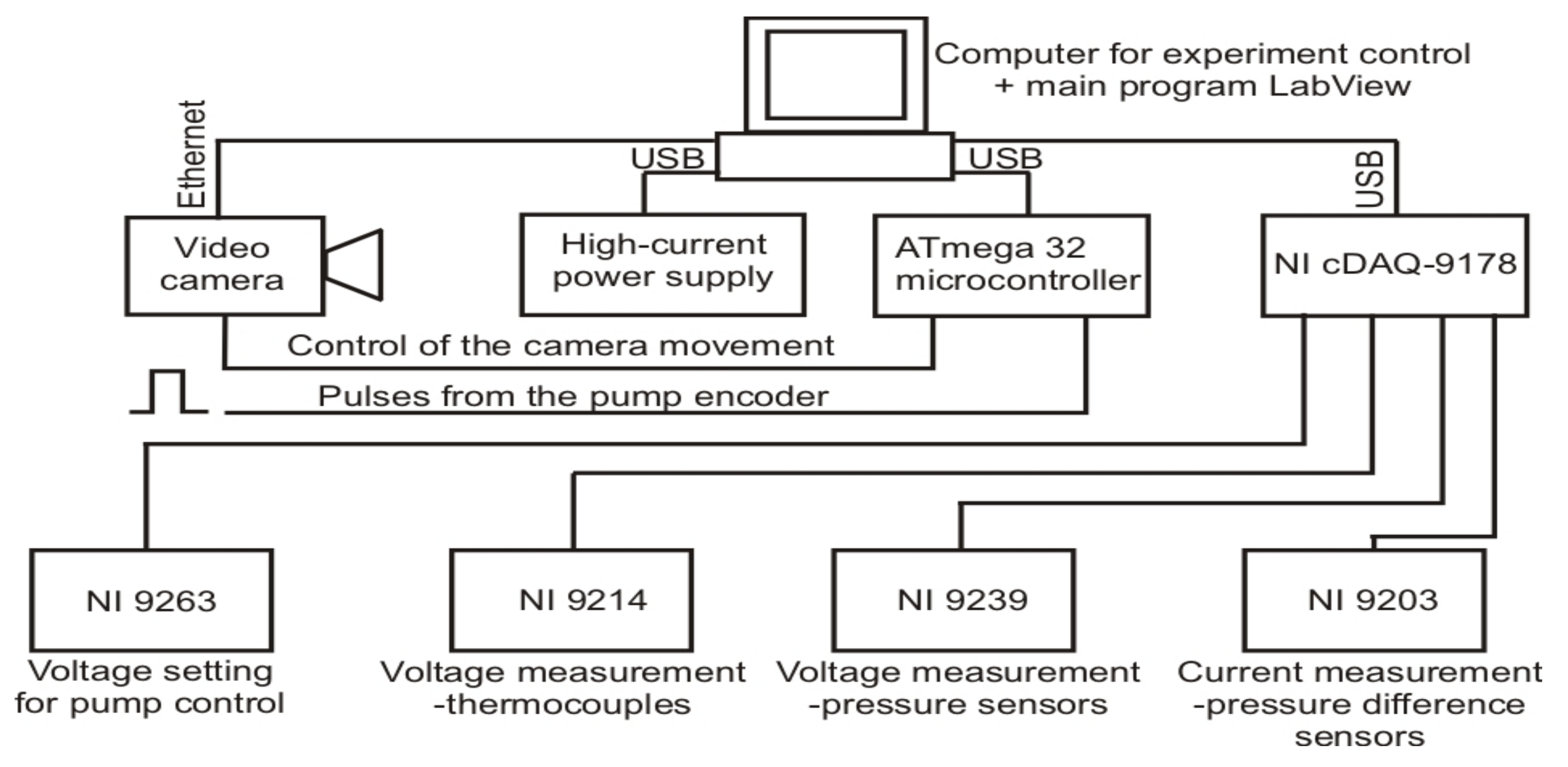
2.1. Design of the Flow Loop, Experimental Equipment and Data Collecting Procedure

The flow loop and its components are presented in Figure 1.
The minichannel, the basic element of the experimental stand (Figure 2), was constructed by glue bonding three transparent glass plates and a cuboid copper block, Figure 3. The cuboid copper block was a solid base for the minichannel and a mass heater as well. Four flat resistance heaters were placed on steel substrates and sintered to the external surface of the copper block. A TDK Lambda GEN 50–30 power supply provided direct current to the heaters, which generated heat required to initiate flow boiling inside the channel (Figure 1 and Figure 2).
Optiwhite glass was selected for the minichannel walls. Optiwhite is colorless, super transparent float glass containing very limited amount of iron and having the highest light-transmission coefficients. Three transparent walls of the channel enabled proper lighting and recording the boiling two-phase structures with a high-speed camera (Phantom 711, Vision Research).
To prevent uncontrolled heating of the flowing fluid by the incandescent light, the LED system of our own design, based on LED diode Citizen CL-L233-HC13L1-C, was applied. LOCTITE® SI 5145 adhesive was used to glue the minichannel elements. The dimensions of the rectangular minichannel, length = 180 mm, width = 4 mm and depth = 1.5 mm, provided a 6 mm2 cross-section and a 2.18 mm hydraulic diameter. Five thermocouples (Czaki TP-201) were mounted, one at the inlet, one at the outlet of the minichannel and three inside the body of the cuboid copper block, Figure 3. Two pressure sensors (Kobold 0–2.5 bar) were placed at the inlet and outlet of the channel. The flow of distilled water was generated by a precision gear pump (Tuthill Concord D) with a maximum capacity of 1.5 × 10⁻⁷ m3/s, featuring very stable laminar flow in the range 43 ≤ Re ≤ 229. Flows at low Reynolds number are quite frequently used in miniature cooling systems of electronic devices.
In the experimental runs, it was necessary to record large numbers of data of various types. Those included video camera images of two-phase flow structures and numeric data of copper block and flowing fluid temperature, fluid pressure and volume flux. Data collection was done by the modular measurement-control system, Figure 4. The core of it was NI cDAQ-9178 chassis (National Instruments) that holds dependent modules, controlling both the measurements of boiling process parameters and the component assemblies, such as the pump, camera triggering, etc.
The following modules comprised the system, as shown in Figure 4: NI cDAQ-9178—the main module, NI 9214—Temperature measurement (CZAKI K-type TP-201 thermocouples), NI 9239—Voltage measurement (KOBOLD pressure sensors, 0–2.5 bar, NI 9203—Current measurement (KOBOLD pressure difference sensors, 0–2.5 bar), NI 9263—Voltage setting for pump control.
In the supplementary measurements of heat loss to the environment, the entire minichannel module was treated as a cuboid with walls of different temperatures measured with the infrared camera. The calculations also accounted for thermal losses from the sight glass. The maximum value of the amount of heat released into the environment in the range of heat fluxes generated in the presented measurements did not exceed 2.1 W, which in relation to the total delivered thermal power was 0.86% to 1.9%. Since the heat losses were minor, they were disregarded in further calculations.

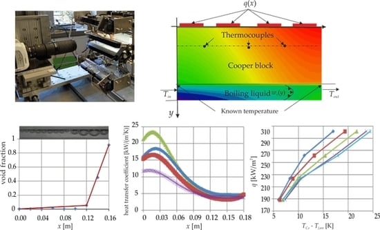
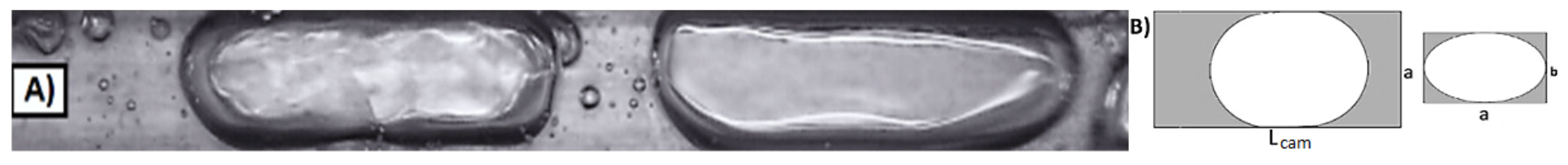
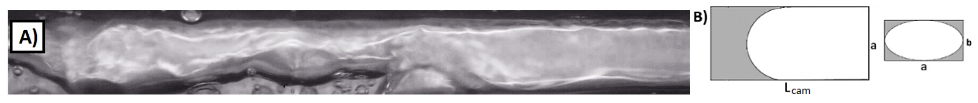
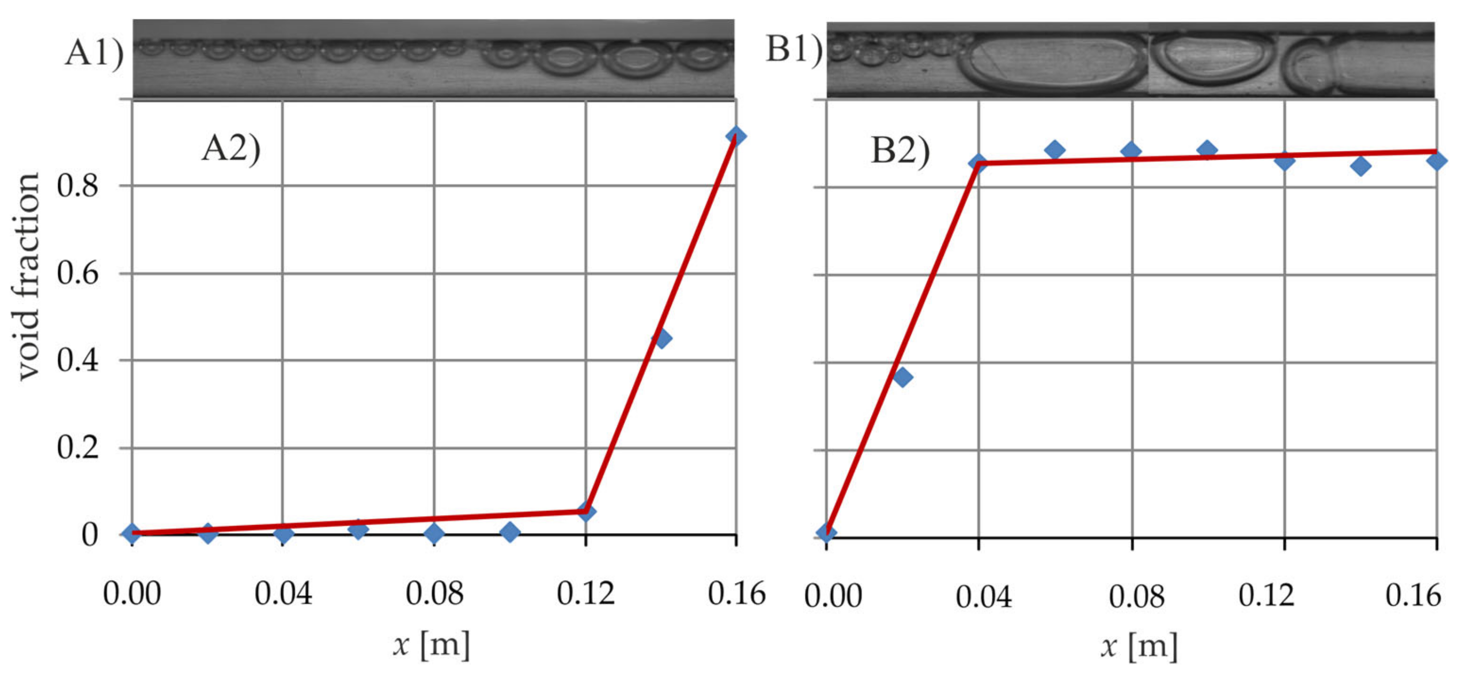
2.2. Procedure of Void Fraction Measurement and Computation in Rectangular Minichannel

Photographs of the observed two-phase flow structures were taken with a high-speed video camera at the recording speed of 7000 fps. The recording speed was selected experimentally to maintain proper exposure and obtain sharp images of dynamic two-phase flow structures. Proper selection of the recording speed is essential for capturing geometric features of the vapor bubbles. The equations approximating spatial geometry of vapor bubbles were applied to convert flat images of bubbles into three dimensional ones, taking simultaneously into account the dimensions of both the bubbles and the minichannel. The shapes of sphere and ellipsoidal cylinder ended with one or two half-ellipsoids were used, depending on inter relations between the dimensions of the bubbles and those of the minichannel. Three cases I, II and III of the characteristic relation between the bubble and minichannel dimensions were specified for void fraction determination in the observed minichannel of length L, width a and depth b, Figure 5, Figure 6 and Figure 7.
Volume of the observed part of the minichannel was:
V = L · a · b ,
  • Small vapor bubbles: Rsb, i ≤ b/2.
The void fraction for small bubbles in the minichannel was calculated from the equation [12]:
φ s b = 4 3 L a b π i A s b , i 3 2 ,
where A s b , i = π R s b , i 2 is the cross sectional area of single spherical bubble.
2.
Large, elongated bubbles, fully visible: ellipse semi-axes P1 lb, i= a/2 and P2 lb, i= b/2.
The void fraction for large, elongated and fully visible vapor bubbles was [12]:
φ l b = i φ l b , i ,
where φ l b , i = L l b , i a π a b 4 + π a 2 b 6 L a b is the void fraction for a single elongated bubble, Llb, i is the bubble length, composed of the length of an ellipsoidal cylinder and two half-ellipsoids.
3.
Large, elongated bubbles, partially visible: ellipse semi-axes P1 lb, i= a/2 and P2 lb, i= b/2.
The void fraction for large, elongated and partially visible vapor bubbles was [12]:
φ l b = i φ l b , i ,
where φ l b , i = L l b , i a 2 π a b 4 + π a 2 b 12 L a b is the void fraction for a single elongated bubble, Llb, i is the bubble length, composed of the length of an ellipsoidal cylinder and one half-ellipsoid.
Three scripts were developed to analyze the void fraction for selected cases of two-phase boiling flow structures found in the recorded videos. MathWorks Matlab and two corresponding toolboxes, computer system vision and image processing, were used for that purpose. By applying the first plan method and the Gaussian model, cases I and II were detected and elaborated with the use of the Vision toolbox). The background subtraction method appeared suitable for case III. Sharpening and pixel multiplication applied for each video frame improved quality of the recorded images. These operations were finally followed by equalization of brightness and contrast of the images to obtain a larger number of details, as shown in Figure 8.
Subsequently the perfected and binarized void frames underwent the following operations: morphologic opening and closing the picture, median filtration from artefacts and morphologic filling of empty spaces in the observed objects—That is vapor bubbles. The application of the entire algorithm converted the image in Figure 8B into the black and white one, Figure 9.
Indexing and measuring procedure was used to get geometric dimensions of each detected bubble. On the basis of these data and with the use of equations presented in this section, by converting the flat picture of the bubble into the expected spatial one, the sought void fraction was calculated in the observed part of the minichannel. The last action of the script was recording the obtained void fraction value for each video frame into a text file for further use.
The estimated values of the void fraction were compared to seven correlations to calculate the void fraction against vapor quality. The results were similar [12]. The maximum scatter did not exceed 16%.

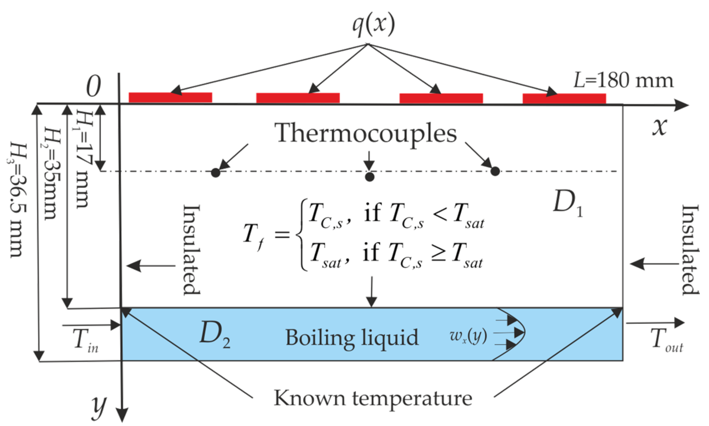
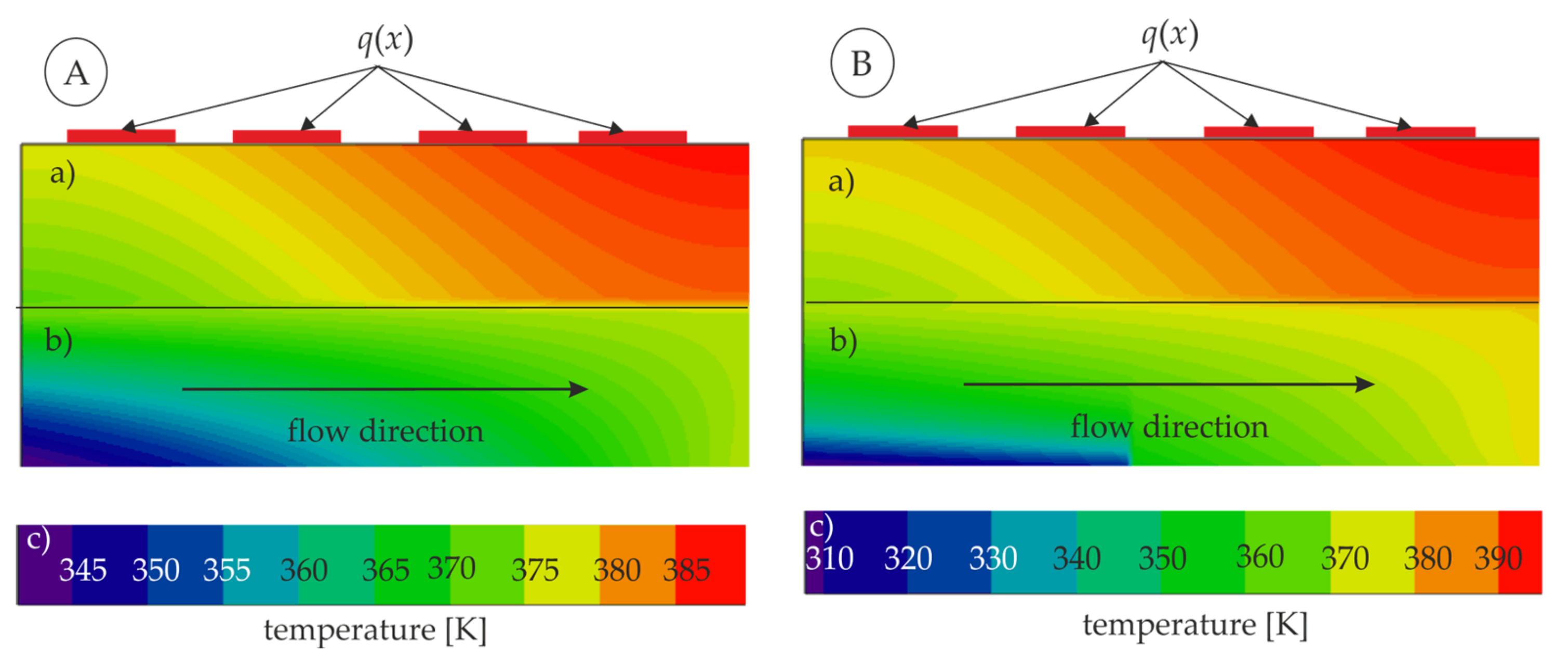
3. Mathematical Model and Numeric Solution

The mathematical model is a modification of the models described earlier in [2,13]. Analysis of the numeric calculation results presented in [13] showed that the change of the temperature along the width of the copper block body was negligible. In the two-dimensional model presented below, the copper block temperature depended only on two variables: y (along its height) and x (in relation to its length). Additionally, this assumption allowed considering heat conduction only in two elements of the measuring module: the copper block and the minichannel with flowing water.
By analogy to [13], we assumed that the heat transfer process in the experimental module was steady-state with constant copper and fluid properties. We also assumed that the temperature of the copper block in domain D 1 = x , y R 2 : 0 < x < L , 0 < y < H 2 satisfied the Laplace equation, i.e.,:
2 T C = 0 .
For Equation (5), we assumed that the temperature of the copper block TC was known at three measuring points (xi, H1), Figure 10.
As in [13], in order to stabilize the numeric calculations two temperature values were added to boundary conditions at both ends of the fluid-copper heater contact surface:
a ) T C 0 , H 2 = 0.5 T i n + T a p p r o x 0 b ) T C L , H 2 = 0.5 T o u t + T a p p r o x L ,
where the broken line approximation of three measured temperatures inside the block, Figure 10, was used to obtain Tapprox. Both vertical walls of the copper block were insulated.
The heat flux q generated by each resistance heater was supplied to the copper block, i.e.,:
λ C T C x , 0 y = q x .
The heat flux q(x) assumed constant values qi, generated by a single heater in the segments, where four resistance heaters were located, Figure 10. Between these segments the heat flux equaled zero:
q ( x ) = q i for x D i , y = 0 0 for x 0 , L D , y = 0 ,
where D = i = 1 4 D i = 2.5 ; 41.5 47.5 ; 86.5 93.5 ; 132.5 139.5 ; 178.5 .
For fluid we assumed that, as shown in Figure 10:
-
The flow in the horizontal minichannel was laminar (Re < 2000) and stationary with a constant volumetric flow rate,
-
Liquid flow in the minichannel was a nonslip flow and the velocity of the fluid had only one non-zero parabolic component wx(y), parallel to the heating block and satisfying the condition:
1 b H 2 H 2 + b w x y d y = w a v e ,
where the wave was known
-
The fluid temperatures at the inlet Tf, in and outlet Tf, out of the minichannel were known,
-
The fluid temperature at the contact with the heater block fulfilled the condition:
T f = T C , s , if T C , s < T s a t T s a t , if T C , s T s a t .
In domain D 2 = x , y R 2 : 0 < x < L , H 2 < y < H 3 , Figure 10, the fluid temperature satisfied the energy equation:
λ f 2 T f = w x y c p ρ f T f x μ f Φ w x y d p d x + Ω x ,
where function Φ = d   w x d y 2 was the Rayleigh dissipation function, pressure gradient d p d x p o u t p i n L = Δ p L and Ω x was negative heat source. The heat flux absorbed by the bubbles, also called a negative heat source, was calculated from the formula, which used experimentally determined void fraction ϕ(x) [14,15,16]:
Ω x = 6 α c o n Δ T 2 R b φ x .
The bubble diameter 2 Rb in subcooled flow boiling was calculated using the correlation proposed in [17]:
2 R b = min 1.4 , 0.6 exp Δ T 45 10 3 .
The convective heat transfer coefficient αcon in Equation (12) was given by Labuncov correlation [18] for laminar flow:
α c o n = λ f 2 R b 0.125 Re 0.65 Pr 1 3
and Δ T was the difference between the fluid temperature Tf in the thermal sublayer δ T and the temperature inside the vapor bubble, which assumed to equal Tsat. Consequently, the fluid superheat Δ T was calculated from the dependence:
Δ T = T f T s a t = q δ T λ f .
In (15) the thermal and hydraulic layer thicknesses were calculated from formulas [16], respectively:
Δ T = T f T s a t = q δ T λ f .   δ T = Pr 1 3 δ h , δ h = 2 μ f w b ρ f ,
where wb(y) = wx(y) and the Fanning friction factor was calculated as in [19]:
f Re f = 24 1 1.3553 b L + 1.9467 b L 2 1.7012 b L 3 + 0.9564 b L 4 0.2537 b L 5 .
The known copper block temperature distributions and the temperature gradient were applied to determine the heat transfer coefficient α x at the copper–fluid interface using the Robin boundary condition:
α x = λ C T C y x , H 2 T C x , H 2 T f , a v e x .
The reference temperature Tf, ave was the average fluid temperature along the depth of the fluid layer equal to the diameter of emerging vapor bubble:
T f , a v e x = 1 2 R b H 2 H 2 + 2 R b T f x , y d y .
The energy Equations (5) and (11) with a set of the adopted boundary conditions led to the solution of two succeeding inverse heat conduction problems (IHCPs) in two domains of different shapes and parameters. The Trefftz method with two sets of adequate T-functions was used to solve the problem.
The boundary conditions Equations (6)–(8) and the harmonic functions (T-functions), defined in [6], were employed to solve Equation (5). Linear combination of T-functions approximated the copper block temperature. These coefficients were found by minimization of the mean square error between the approximated temperature and the boundary conditions. T-functions for homogeneous energy equation, corresponding to energy Equation (11) were applied to find the flowing fluid temperature [20].
The fluid temperature was approximated by a sum of particular solution of Equation (11) and the linear combination of the T-functions shown in [9]. Similar to the case of copper block temperature, the boundary conditions for the fluid were adopted to compute the coefficients of that linear combination.

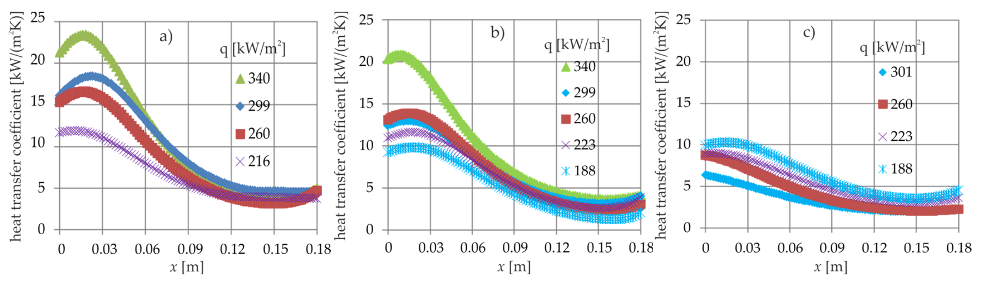
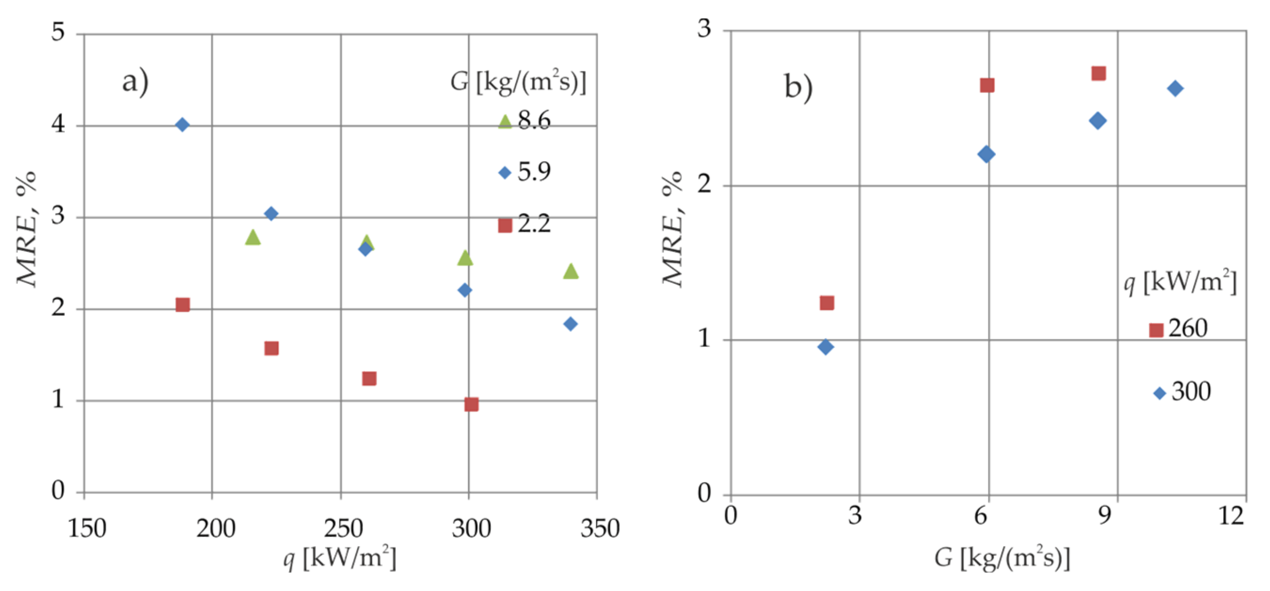
4. Results and Discussion

The measurement procedure included recording the following quantities: temperature and pressure at the channel inlet and outlet, differences in inlet and outlet pressures, volume flux of the flowing medium, temperature at three selected points inside the copper block and also current and voltage of the heater power supply. The measurements were taken for the following ranges of the experimental parameters: total heat flux generated by four external flat heaters 188 ≤ q ≤ 340 kW/m2, inlet pressure 1.05 ≤ p ≤ 1.17 bar (practically constant), inlet fluid subcooling 3.6 ≤ Δ T ≤ 70.7 K and mass flux 2.2 ≤ G ≤ 8.6 kg/(m2 s), 43 ≤ Re ≤ 229.
At the same time, flow boiling in the minichannel was filmed using high-speed video camera and local void fractions φ(x) were measured on the basis of recorded images. The scripts developed in Section 2.2 allowed the calculation of the void fraction for each pattern of two-phase flow structures observed in this study. The experimental local values of the void fraction, measured along the minichannel length, were approximated with broken lines, as shown in Figure 11.
The results of numeric calculations presented in Figure 12 were obtained for experimental parameters given in Section 4. In the first step, nine T-complete functions were used to calculate the approximate two-dimensional temperature of the copper block TC for Equation (5). Next, by combining four T-complete functions for Equation (20) and particular solution of Equation (11), the field of the fluid temperature Tf was found.
Fluid flowing into the minichannel substantially reduces the temperature of the copper block across the contact area, Figure 12. The fluid motion in the minichannel causes heat transfer in the direction of its axis. As a result, the temperature in the entire channel increases as does the void fraction, which impairs heat transfer between the fluid and the heater. For this reason, in the final section of the module, both the liquid temperature and the heater temperature increase significantly.
The temperature distribution in both the fluid and the heating block, Figure 12, is as expected, the isotherms run in a manner likely for the direction and intensity of flow and location of the heaters. The charts are not fully comparable, because both parameters, G and q, are different for each case, but the impact of the parameter change on the temperature field is clear.
The results of numeric calculations presented in Figure 12 were obtained for experimental parameters given in Section 4. In the first step, nine T-complete functions were used to calculate the approximate two-dimensional temperature of the copper block TC for Equation (5). Next, by combining four T-complete functions for Equation (20) and particular solution of Equation (11), the field of the fluid temperature Tf was found.
The boundary conditions adopted for the copper block and liquid temperatures were satisfied with high accuracy. The maximum differences between the calculated and measured temperatures of the copper block did not exceed 24 K (5.93%) for the first measuring point (from the inlet to the minichannel), 19 K (4.45%) for the second and 16 K (3.72%) for the third measurement point. Throughout the study, the largest errors were always at the first measuring point and the smallest at the last. When identifying the liquid temperature, the maximum differences between the calculated and measured temperature did not exceed 13 K (3.71%) at the inlet to the minichannel and 15 K (4.65%) at the outlet from the minichannel. As in the case of thermocouples placed in the copper block, the differences between the measured and calculated temperatures for liquids at the inlet to the minichannel were in most cases higher than the differences at the outlet from the minichannel.
Variation of the heat transfer coefficient for the flowing two-phase mixture is shown in Figure 13 as the function of the distance from the minichannel inlet. It is presented for three selected mass fluxes and varying heat flux. The heat transfer coefficient decreases as the distance from the inlet grows, which is related to increasing void fraction. Some variation in this trend can be observed both at the channel inlet and outlet. The growing heat flux also increases the heat transfer coefficient. Analysis of graphs in Figure 13 shows a known pattern—an increase in flow intensity causes an increase in heat transfer coefficient.
In the initial segment of the minichannel, changes in the calculated values of heat transfer coefficients as a function of distance from the inlet, Figure 13, are non-physical in nature. This is the result of boundary condition (6) adopted to stabilize the numeric procedure.
The shape of boiling curves presented in Figure 14 for various distances from the minichannel inlet is similar to the initial section of standard boiling curve. The curves originate with segments of steep dependence of the heat flux q versus the temperature difference TC, sTsat and flatten with further increase of that difference. This results from the growing vapor phase (void fraction) and approaching first boiling crisis. In the discussed experiment, the vapor was not superheated to prevent possible thermal damage of the research facility. Therefore, the boiling curves are limited to their initial segments.
The smaller the distance from the inlet, the greater is the heat flux q for the same temperature difference between the heating surface and the boiling liquid. This result agrees qualitatively with the results shown in Figure 13, because the heat transfer coefficient increases with the decreasing distance to the inlet.
With increasing distance from the channel inlet, the temperature difference TC, sTsat must increase to induce heat transfer of expected value. This is due to the increase in the amount of gaseous phase in the two-phase mixture and thus in its insulating properties.
The uncertainties of the experimental parameters determined in study [2] were applied to calculate the mean relative error (MRE) of the heat transfer coefficient α (x). Figure 15 shows the MRE as a function of both heat flux and mass flux. When the heat flux supplied to the copper block increases, the MRE decreases from the value of 4.2% for heat flux q = 188 kW/m2 down to 1.0% for q = 340 kW/m2. For smaller mass fluxes, the MRE values are lower.

5. Conclusions

The experimental data gained at the Warsaw University of Technology, Plock Campus created a ground for the completed numeric analysis. The design of the experimental setup allowed setting and automatically acquiring temperature of the copper block and flowing fluid, fluid pressure, volumetric flow rate, heat flux and video recording for various positions of the video camera along the minichannel length. During the experimental run the research schedule of the setup was under control of the program created in the LabView environment. Data acquisition was controlled by the same script as well. The configuration of the setup is flexible enough to provide the potential for further expansion of the research program for new settings of thermal and flow parameters, channel space orientations and channel geometry.
The unique feature of the photographic method developed in this research is the video registration of the observed two-phase flow structure coupled with the measurement of the corresponding local value of the void fraction. This idea is based on the conversion of the flat image of the vapor bubble into the expected spatial shape. The obtained values of the void fraction were successfully applied in boiling two-phase flow modeling and numeric calculations. Disadvantages of the photographic method include 1) the requirement of quick collection of a large amount of data and 2) laborious conversion and refinement of the data into the required void fraction values with dedicated Matlab scripts.
The mathematical approach to solving two sequential IHCPs in flow boiling in the asymmetrically heated rectangular and horizontal minichannel was validated against experimental data. The employed meshless Trefftz method, making use of two types of T-complete functions, allowed obtaining approximate solutions of two coupled energy equations with their boundary conditions. The method provided stable solution of IHCP and consequently granted determination of: 1) the two-dimensional temperature distributions in two contacting domains, having different shapes and thermal features (copper block and flowing fluid), 2) the heat flux transferred from the block to the flowing two-phase mixture, and 3) the heat transfer coefficient on the contact surface between the copper block and flowing fluid. The Trefftz method is not limited by the number or character of boundary conditions. They can be established directly from temperatures or temperature gradients and they may have continuous or discrete form as well. It is worth noting that the approximate solutions satisfy the governing partial differential equations exactly and numeric calculations are not very much complicated because T-complete functions are polynomials in the investigated case.
In the near future the research program will be extended to include water, ethanol and FC72 and various minichannel space orientations [21].

Author Contributions

Conceptualization, S.H., M.E.P.; methodology, M.G, K.P., S.H. and B.M.; validation, S.H., B.M.; formal analysis, S.H.; investigation, M.G. and K.P.; writing—Original draft preparation, M.G., S.H. and M.E.P.; writing—Review & editing, S.H., B.M. and M.E.P.; funding acquisition, M.G. All authors have read and agreed to the published version of the manuscript.

Funding

The research was funded by the Warsaw University of Technology, Plock Campus, grant no. 504/04480/7193/44.000000 and the Poland National Science Center, grant no. UMO-2018/31/B/ST8/01199.

Conflicts of Interest

The authors declare no conflicts of interest.

Nomenclature

Nomenclature
Aarea, cross-section, m2
achannel width, m
bchannel depth, m
cpspecific heat, J/(kgK)
Ddomain, mm
fFanning friction factor
Gmass flux, kg/(m2 s)
Hheight, m
Llength, m
MREmean relative error
ppressure, Pa
Pellipse semi-axis, m
PrPrandtl number
qheat flux, kW/m2
Rradius, m
ReReynolds number
Ttemperature, K, °C
wvelocity, m/s
xcoordinate in the flow direction, m
ycoordinate perpendicular to the flow direction, m
Vvolume, m3
2 = 2 x 2 + 2 y 2 Laplacian in Cartesian coordinates
Greek symbol
αheat transfer coefficient, W/(m2 K)
Δdifference
ΦRayleigh dissipation function, s-2
ϕvoid fraction
λthermal conductivity, W/(m K)
μdynamic viscosity, Pa s
ρdensity, kg/m3
Ωnegative heat source, W/m3
Subscripts
approxapproximation
aveaverage
bbubble
Ccopper block
camobserved part of the minichannel
conconvection
ffluid
hhydraulic
ii–th bubble,
ininlet
lblarge bubble
outoutlet
ssurface
satsaturation
sbsmall bubble
Tthermal
Xin the flow direction

References

  1. Kim, S.-M.; Mudawar, I. Review of databases and predictive methods for heat transfer in condensing and boiling mini/micro-channel flows. Int. J. Heat Mass Transf. 2014, 77, 627–652. [Google Scholar] [CrossRef]
  2. Grabowski, M.; Hożejowska, S.; Poniewski, M.E. Trefftz method-based identification of heat transfer coefficient and temperature fields in flow boiling in an asymmetrically heated rectangular mini-channel. In Proceedings of the XV Symposium on Heat and Mass Transfer 2019 (SOHAMT 2019), Kołobrzeg, Poland, 16–19 September 2019; Volume 1, pp. 179–192. [Google Scholar]
  3. Karayiannis, T.G.; Mahmoud, M.M. Flow boiling in microchannels: Fundamentals and applications. Appl. Therm. Eng. 2017, 115, 1372–1397. [Google Scholar] [CrossRef]
  4. Płaczkowski, K.; Poniewski, M.E.; Grabowski, M.; Alabrudziinski, S. Photographic technique application to the determination of void fraction in two-phase flow boiling in minichannels. Appl. Mech. Mater. 2015, 797, 299–306. [Google Scholar] [CrossRef]
  5. Saisorn, S.; Kaew-On, J.; Wongwises, S. Flow pattern and heat transfer characteristics of R-134a refrigerant during flow boiling in a horizontal circular mini-channel. Int. J. Heat Mass Transf. 2010, 53, 4023–4038. [Google Scholar] [CrossRef]
  6. Trefftz, E. Ein Gegenstück zum Ritzschen Verfahren. In Proceedings of the International Kongress für Technische Mechanik, Zürich, Switzerland, 12–17 September 1926; pp. 131–137. [Google Scholar]
  7. Piasecka, M.; Hożejowska, S.; Poniewski, M.E. Experimental evaluation of flow boiling incipience of subcooled fluid in a narrow channel. Int. J. Heat Fluid Flow 2004, 25, 159–172. [Google Scholar] [CrossRef]
  8. Hożejowska, S.; Piasecka, M.; Poniewski, M.E. Boiling heat transfer in vertical minichannels. Liquid crystal experiments and numerical investigations. Int. J. Therm. Sci. 2009, 48, 1049–1059. [Google Scholar] [CrossRef]
  9. Hożejowska, S.; Kaniowski, R.; Poniewski, M.E. Trefftz method for calculating temperature field of the boiling liquid flowing in a minichannel. Int. J. Numer. Methods Heat Fluid Flow 2014, 24, 811–824. [Google Scholar] [CrossRef]
  10. Grabowski, M.; Hożejowska, S.; Pawinska, A.; Poniewski, M.E.; Wernik, J. Heat Transfer Coefficient Identification in Mini-Channel Flow Boiling with the Hybrid Picard-Trefftz Method. Energies 2018, 11, 2057. [Google Scholar] [CrossRef] [Green Version]
  11. Fan, C.-M.; Chan, H.-F.; Kuo, C.-L.; Yeih, W. Numerical solutions of boundary detection problems using modified collocation Trefftz method and exponentially convergent scalar homotopy algorithm. Eng. Anal. Bound. Elem. 2012, 36, 2–8. [Google Scholar] [CrossRef]
  12. Płaczkowski, K. Application of Photographic Technology to the Two-Phase Flow Regime Recording and Concurrent Void Fraction Quantification (In Polish). Ph.D. Thesis, Warsaw University of Technology, Płock, Poland, 2020. [Google Scholar]
  13. Hożejowska, S.; Grabowski, M.; Poniewski, M.E. Implementation of a three-dimensional model for the identification of flow boiling heat transfer coefficient in rectangular mini-channel. In Proceedings of the International Conference on Experimental Fluid Mechanics, Franzensbad, Czech Republic, 19–22 November 2019; Dančová, P., Ed.; Technical University of Liberec and MiTpp: Liberec, Czech Republic, 2001; pp. 178–182. [Google Scholar]
  14. Bilicki, Z. Latent heat transport in forced boiling flow. Int. J. Heat Mass Transf. 1983, 26, 559–565. [Google Scholar] [CrossRef]
  15. Bilicki, Z. The relation between the experiment and theory for nucleate forced boiling, Invited lecture. In Proceedings of the 4th ExHFT, Brussels, Belgium, 2–6 June 1997; pp. 571–578. [Google Scholar]
  16. Bohdal, T. Modeling the process of bubble boiling on flows. Arch. Thermodyn. 2000, 21, 34–75. [Google Scholar]
  17. Tolubinski, V.I.; Kostanchuk, D.M. Vapour bubbles growth rate and heat transfer intensity at subcooled water boiling. In Proceedings of the 4th International Heat Transfer Conference, Paris-Versailles, France, 31 August–5 September 1970; pp. 1–11. [Google Scholar]
  18. Labuncov, D.A. Obobščennyie zavisimosti dla teplootdači pri puzirkovom kipenii židkosti. Teploenergetika 1960, 5, 76–81. [Google Scholar]
  19. Shah, R.K.; London, A.L. Laminar Flow Forced Convection in Ducts; Academic Press: New York, NY, USA, 1978. [Google Scholar]
  20. Hożejowski, L.; Hożejowska, S. Trefftz method in an inverse problem of two-phase flow boiling in a minichannel. Eng. Anal. Bound. Elem. 2019, 98, 27–34. [Google Scholar] [CrossRef]
  21. Layssac, T.; Lips, S.; Revellin, R. Effect of inclination on heat transfer coefficient during flow boiling in a mini-channel. Int. J. Heat Mass Transf. 2019, 132, 508–518. [Google Scholar] [CrossRef]
Figure 1. Flow loop. 1—Measurement module with the minichannel (details in Figure 3), 2—Heating copper block, 3—Temperature and pressure sensors, 4 DC power supply, 5—Cooler with ventilator, 6—Rotameter, 7—Filter, 8—Pump, 9—Pressure control, 10—Compressed air valves, 11—Compressed air tank, 12—Preheater, 13—Facility control unit, 14—Computer for experiment control + LabView software, 15—High speed camera, Pca—Compressed air pressure sensor.
Energies 13 03973 g001
Figure 2. General view of the experimental stand; labels as in Figure 1.
Energies 13 03973 g002
Figure 3. Copper block with attached glass minichannel and location scheme of resistance heaters and thermocouples—Transverse section and axonometric view; dimensions in mm (pictorial view, not to scale).
Energies 13 03973 g003
Figure 4. Block diagram of the data flow and control system.
Energies 13 03973 g004
Figure 5. (A) Actual and (B) approximated shapes of vapor bubbles in longitudinal and transverse sections of the channel with flow direction, case I. Water, Tin = 63.1 °C, Tout = 123.8 °C, pin = 1.165 bar, Δp = 0.0024 bar, q = 298.7 kW/m2, G = 7.2 kg/(m2 s), Re = 55.0, Lcam = 20 mm.
Energies 13 03973 g005
Figure 6. (A) Actual and (B) approximated shapes of vapor bubbles in longitudinal and transverse sections of the channel with flow direction, case II. Water, Tin = 55.2 °C, Tout = 125.9 °C, pin = 1.0697 bar, Δp = 0.0016 bar, q = 260.1 kW/m2, G = 8.6 kg/(m2 s), Re = 66.9, Lcam = 20 mm
Energies 13 03973 g006
Figure 7. (A) Actual and (B) approximated shapes of vapor bubbles in longitudinal and transverse sections of the channel with flow direction, case III. Water, Tin = 72 °C, Tout = 120 °C, pin = 1.147 bar, Δp = 0.0016 bar, q = 270.5 kW/m2, G = 5.9 kg/(m2 s), Re = 43.5, Lcam = 20 mm.
Energies 13 03973 g007
Figure 8. Picture of two-phase flow (A) before and (B) after the operations improving its quality.
Energies 13 03973 g008
Figure 9. Image of two-phase flow resulting from morphologic operations.
Energies 13 03973 g009
Figure 10. Scheme of the experimental stand with the adopted boundary conditions; (pictorial view, not to scale).
Energies 13 03973 g010
Figure 11. Examples of recorded flow structures presented in (A1): q = 298.8 kW/m2, G = 8.6 kg/(m2 s); (B1): q = 223.2 kW/m2, G = 2.2 kg/(m2 s). Corresponding void fractions (blue points), approximated with broken lines (red lines), are shown in (A2) and (B2).
Energies 13 03973 g011
Figure 12. Two-dimensional temperature fields of (a) the copper block and (b) flowing fluid obtained by the Trefftz method for (A) heat flux q = 223.2 kW/m2 and mass flux G = 5.9 kg/(m2 s) and (B) heat flux q = 340 kW/m2,mass flux G = 5.9 kg/(m2 s), (pictorial view, not to scale).
Energies 13 03973 g012
Figure 13. Heat transfer coefficient as a function of minichannel length (a) for G = 8.6 kg/(m2s), (b) G = 5.9 kg/(m2 s) and (c) G = 2.2 kg/(m2s).
Energies 13 03973 g013
Figure 14. Boiling curves for selected points x along the minichannel length for (a) G = 2.2 kg /(m2 s), (b) G = 5.9 kg /(m2 s) and (c) G = 8.6 kg /(m2 s).
Energies 13 03973 g014
Figure 15. Mean relative error vs. (a) heat flux q, and (b) mass flux.
Energies 13 03973 g015

