Forecasting Day-Ahead Hourly Photovoltaic Power Generation Using Convolutional Self-Attention Based Long Short-Term Memory


1
Department of Information and Communication Engineering, Inha University, Incheon 22212, Korea
2
College of Computing, Georgia Institute of Technology, Atlanta, GA 30332, USA
*
Author to whom correspondence should be addressed.
Energies 2020, 13(15), 4017; https://0-doi-org.brum.beds.ac.uk/10.3390/en13154017
Submission received: 30 June 2020
/
Revised: 25 July 2020
/
Accepted: 31 July 2020
/
Published: 4 August 2020
(This article belongs to the Special Issue Machine Learning and Optimization with Applications of Power System II)
Abstract
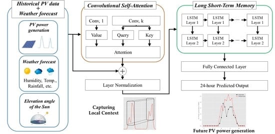
:The problem of Photovoltaic (PV) power generation forecasting is becoming crucial as the penetration level of Distributed Energy Resources (DERs) increases in microgrids and Virtual Power Plants (VPPs). In order to improve the stability of power systems, a fair amount of research has been proposed for increasing prediction performance in practical environments through statistical, machine learning, deep learning, and hybrid approaches. Despite these efforts, the problem of forecasting PV power generation remains to be challenging in power system operations since existing methods show limited accuracy and thus are not sufficiently practical enough to be widely deployed. Many existing methods using long historical data suffer from the long-term dependency problem and are not able to produce high prediction accuracy due to their failure to fully utilize all features of long sequence inputs. To address this problem, we propose a deep learning-based PV power generation forecasting model called Convolutional Self-Attention based Long Short-Term Memory (LSTM). By using the convolutional self-attention mechanism, we can significantly improve prediction accuracy by capturing the local context of the data and generating keys and queries that fit the local context. To validate the applicability of the proposed model, we conduct extensive experiments on both PV power generation forecasting using a real world dataset and power consumption forecasting. The experimental results of power generation forecasting using the real world datasets show that the MAPEs of the proposed model are much lower, in fact by 7.7%, 6%, 3.9% compared to the Deep Neural Network (DNN), LSTM and LSTM with the canonical self-attention, respectively. As for power consumption forecasting, the proposed model exhibits 32%, 17% and 44% lower Mean Absolute Percentage Error (MAPE) than the DNN, LSTM and LSTM with the canonical self-attention, respectively.
1. Introduction
Microgrids and Virtual Power Plants (VPPs) are two remarkable solutions for a reliable supply of electricity in a power system [1]. Microgrids are power systems comprising Distributed Energy Resources (DERs) and electricity end-users, possibly with controllable elastic loads, all deployed across a limited geographic area [2]. The concept of VPP was proposed in [3]. A VPP is a flexible representation of a portfolio of DERs that can be used to make contracts in the wholesale market and to offer services to the system operator [4]. The increasing penetration of intermittent and variable renewable energy resources (e.g., wind and solar) has significantly complicated energy system management for microgrids and a VPP [5,6]. For the above reasons, PV power generation forecasting is an important and challenging topic for the fields of microgrids and VPPs.
The PV power generation, a key renewable energy source for microgrids and VPPs, is a power generation method that produces electricity by converting sunlight into direct current electricity. The amount of sunlight is bound to depend on weather conditions. In other words, the amount of PV power generation also depends on meteorological variables such as solar radiation, temperature, cloud changes, wind speeds and relative humidity. Therefore, there are difficulties in predicting the exact amount of PV power generation [7,8].
In this context, many previous studies have tried to increase the accuracy of PV power forecasts, mainly by using weather data from the past [9,10,11,12,13,14]. These previous studies constructed prediction models by using or combining Convolution Neural Network (CNN) and Long Short-Term Memory (LSTM), independently. Although these approaches used canonical self-attention mechanisms to emphasize important features of data, they might generate inappropriate keys and queries that do not fit the local context. To address this problem, we propose a LSTM based forecasting model using convolutional self-attention. The proposed model adopts the convolution-self attention mechanism to solve the problems of the existing self-attention mechanism by generating keys and queries that fit the local context [15]. In addition, we do not use only historical data but also future data to further improve prediction accuracy.
The rationale of the proposed Convolutional Self-Attention LSTM model design is to combine the efficiency of attention in generating the keys and queries that fit the context information with the ensemble potential of multi-LSTM by introducing a convolutional self-attention-based context learning approach.
The rest of the paper is organized as follows: In Section 2, we introduce related researches on Photovoltaic (PV) forecasting and describe the structure of two deep learning-based models for performance comparisons with the proposed model. The detailed input and output of the proposed model are explained in Section 3. Section 4 describes the proposed model, and Section 5 shows the results of the experiment. Lastly, Section 6 concludes the paper.
2. Related Work
In the existing PV power generation prediction research, the forecast horizons varied from minutes to months depending on their usage. In addition, they used various forms of input data, such as using only historical PV power generation, using historical PV power generation and weather data, and using only weather forecasts. The methods for modeling the above data mainly include statistical methods, machine learning and deep learning methods. Statistical approaches include the Autoregressive Moving Average (ARMA) and the Autoregressive Integrated Moving Average (ARIMA). Machine learning and deep-learning approaches include the Support Vector Machine (SVM), Artificial Neural Network (ANN), Deep Neural Network (DNN), Recurrent Neural Network (RNN), Convolution Neural Network (CNN) and Long Short-Term Memory (LSTM). In addition, hybrid methods such as SVM-ARIMA and Hybrid PSO-ELM (Particle Swarm Optimization Algorithm-Extreme Learning Machine) are used [16].
A study for predicting 1-h ahead using the historical PV data through ARIMA was conducted in [17] and showed the results of average MAE (Mean Absolute Error) of 0.0206 kW. In [18], the authors proposed an ARMAX model for applying climate information data to ARIMA and showed the results of MAPE (Mean Absolute Percentage Error) of 82.69%. The historical power, weather forecasting data were used for 1-day ahead forecasting and modeled with the proposed ARMAX method. Zeng et al. proposed the SVM based model for 1-h head forecasting, using meteorological data such as sky cover, relative humility, and wind speed [19] and showed the results of MAPE of 15.6% in Denver and 26.25% in Seattle. There are two PV power forecasting models using ANN [20,21]. These studies used the same ANN method, but the temporal horizons they needed to predict, and the input data used, were different. In [20], the authors used the historical power, cell temperature, and solar radiation for 24-h ahead foresting and showed the results of MAPE of 1.92% on sunny days, 2.30% on partly cloudy days, 5.28% on overcast days. Meanwhile, the authors in [21] used the historical PV energy generation and weather forecast data from Numerical Weather Prediction (NWP) for up to 39-h ahead forecasting and showed the results of MAE of 7.01%. Son, J. et al., conducted a task for 1-day ahead forecasting, training PV power and weather data using a six-layer feedforward deep neural network [22] and showed the results of MAE of 2.9%. Then they verified it using weather forecasting data in the testing process. Abdel-Nasser et al. proposed a deep LSTM by using historical power data for 1-h ahead forecasting [23] and showed the results of RMSE (Root Mean Squared Error) of 82.15. Qing and Niu et al. applied the LSTM model using weather forecast data for 1-day ahead solar irradiance forecasting [24]. The RMSE value of the model in [24] was 76.245 (). A high-precision deep neural network model named PVPNet to forecast 24-h PV system output power was proposed in [25]. In this paper, the authors used deep neural networks, which were able to generate a 24-h probabilistic and deterministic forecasting of PV power output based on meteorological information such as temperature, solar radiation and historical PV system output data. This PVPNet showed the results of MAE of 109.4845 (W). In [26], the authors proposed a GT-DBN (Gray Theory-based data preprocessor Deep Belief Network) that predicts PV output over a prediction time of over 24 h by integrating a gray theory and DBN-based data preprocessor with a supervised learning system. The GT-DBN showed better prediction results compared with other models and showed the results of MAPE of 3.76%. The long-term PV power generation prediction for one year was studied in [27]. In this paper, the authors used a predictive model that ensembles meta runners (VAR (Vector Autoregression), ARIMA, LSTM) and CNN, and showed the results of MAE of 16.70 (MWh). Bouzerdoum et al. used the historical power for 1-h ahead forecasting and modeled by combining SVM and SARIMA (Seasonal Autoregressive integrated moving average) [28] and showed the results of NRMSE (Normalized Root Mean Absolute Error) of 9.4010%. Behera et al. used the historical solar irradiance, air temperature for 15-min, 30-min, and 60-min ahead forecasting, and proposed a model that optimizes ELM with adaptive PSO methods [29] and showed the results of MAPE of 1.44%.
Compared with the existing works, our proposed method has two prominent advantages. First, our method adopts the convolutional self-attention to efficiently model local context of input data. Second, we use both historical and future data for day-ahead hourly PV power forecasting to enhance the prediction accuracy.
2.1. DNN Based Approach to Predict PV Power Generation
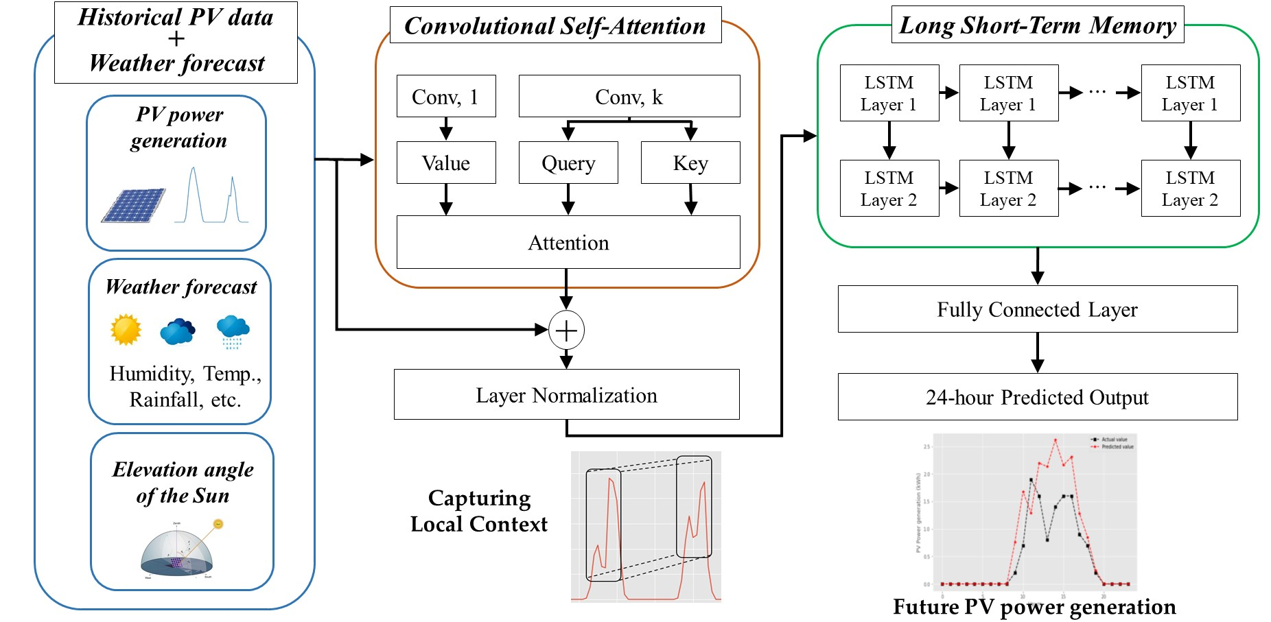
MLP (Multi-Layer Perceptron) is a calculation method that uses a huge number of artificial neurons and consists of an input layer, an output layer, and one or several hidden layers between them [30]. If there are two or more hidden layers, it is generally referred to as DNN. After forming a network with a fixed number of neurons, the training process involves finding the relationship between input and output data. Figure 1 shows the architecture of the DNN based model that was used to predict PV power generation. represents the -th node of layer , while represents the number of nodes of layer . On the other hand, represents the weight between the -th node of layer and the q-th node of layer . In designing the DNN model in this paper, three hidden layers were constructed and .
2.2. LSTM-Based Approach to Predict PV Power Generation
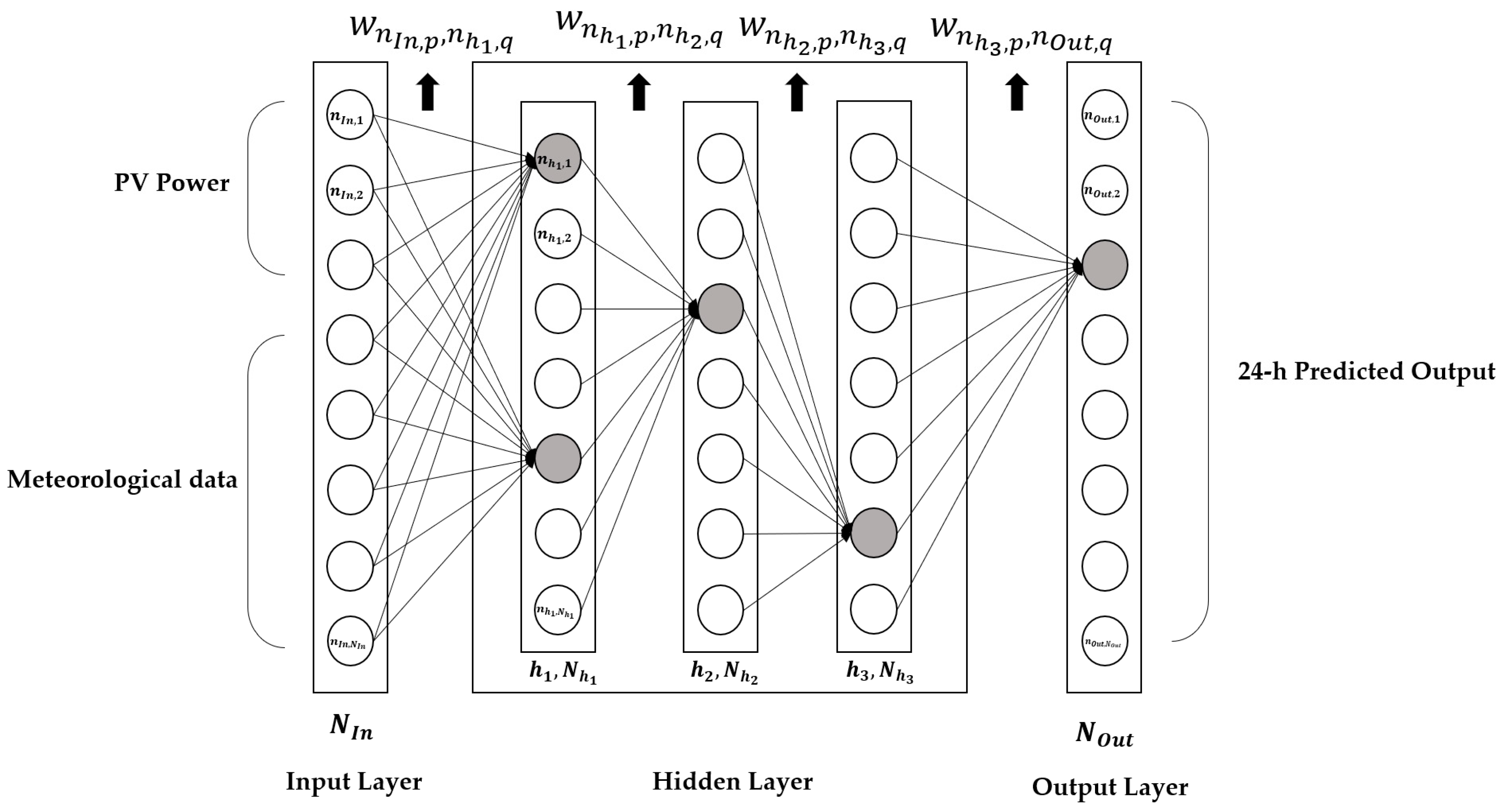
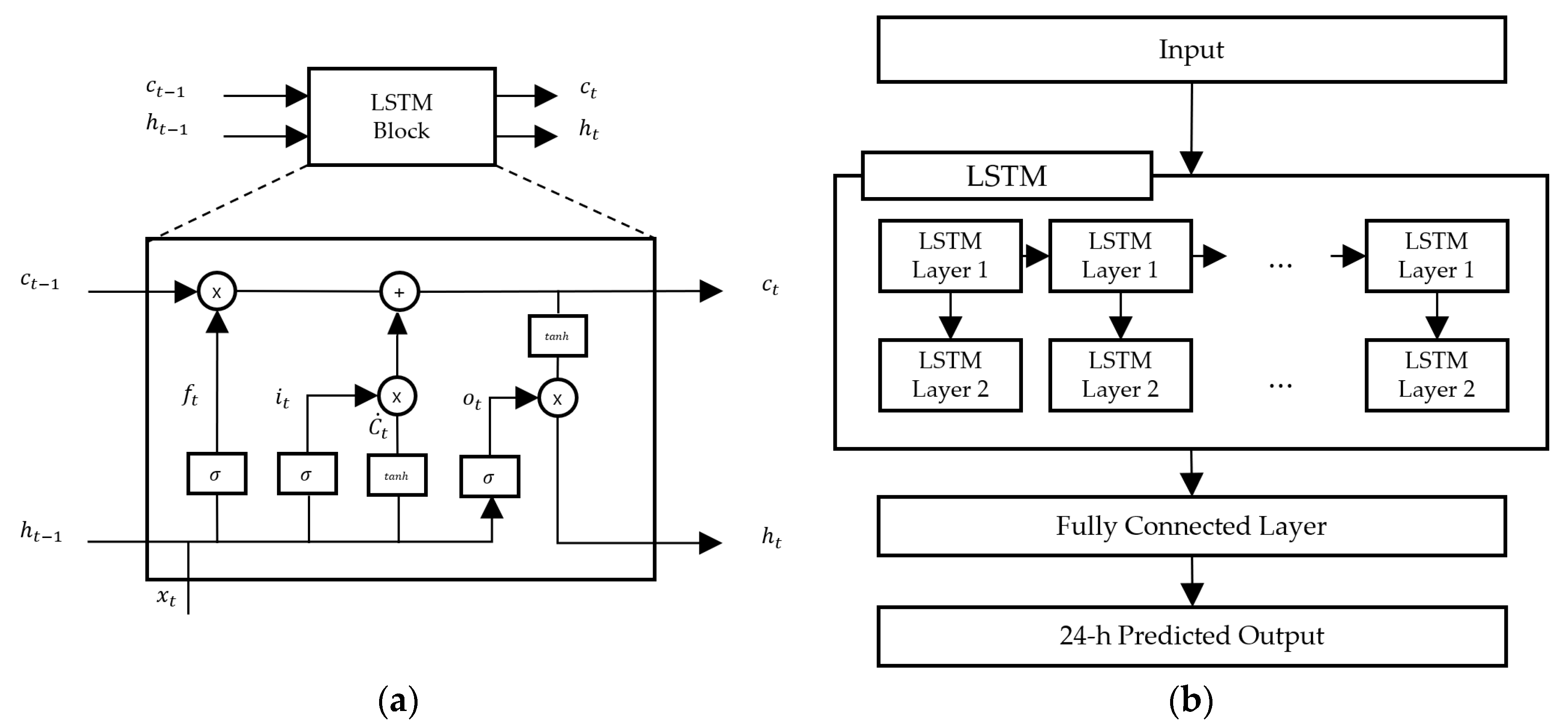
RNN is proposed to model a time series using an autoregressive method [31,32]. However, RNN has difficulty in training due to the problem of gradient vanishing and exploding [33]. The proposed RNN is a special kind; LSTM and gradient clipping solve the problem of gradient vanishing and extension and also solve the complex and artificial long-term dependency problem [34]. In Figure 2, (a) shows the interior of the LSTM block and (b) shows the LSTM-based model architecture to predict PV power generation. In Figure 2b, two layers of LSTM layers are stacked, and each LSTM layer has 256 units and is designed to output prediction results for the future 24-h through a fully connected layer.
3. Data Processing
3.1. Features and Their Notations
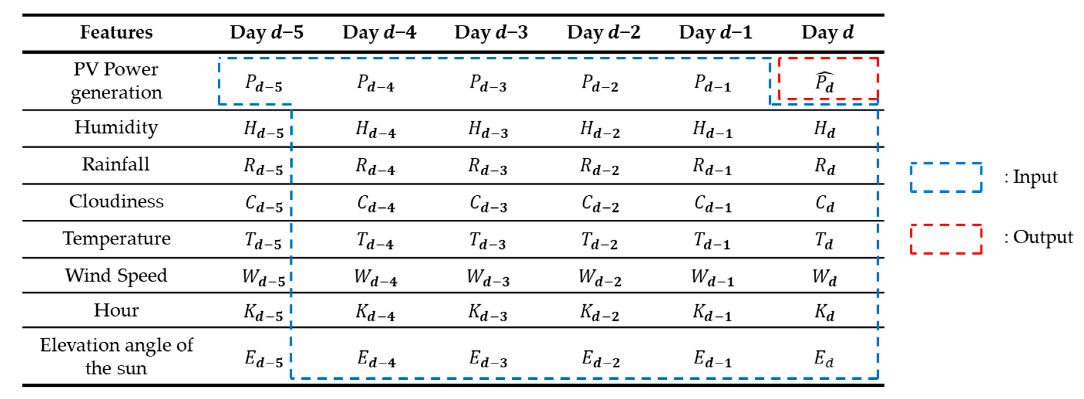
In this paper, we aim to perform a day-ahead hourly forecasting task using both historical and future data. We consider PV power generation and weather measurements as historical data and weather forecast data as the future data. Since we use the historical data and future data, we need to extract common features of weather measurement data and weather forecast data. To do this, we use the humidity, rainfall, cloudiness, temperature and wind speed data. Table 1 shows the notation for the measurement corresponding to each feature of each day.
We use the hourly data on the elevation angle of the sun on each day and the Hour value as shown in Table 1. Since the elevation angle of the sun is calculated by the formula in [35], we can use the future elevation angle of the sun without forecasting. Equation (1) indicates the elevation angle of the sun.
where is a declination of the sun, is a latitude and H is an hour angle.
Note that each feature consists of 24-h values. means a set of PV power generation values for 24 h on n-th days and means the PV power generation value on day n at t-hour. (). For example, is the PV power generation values from 0:00 to 23:00 on day 3, and is the PV power generation value at 5:00 on day 3. The same rules apply to the rest of the features.
In this paper, we construct the input using the past 5 days of PV power generation to predict day-ahead hourly PV power generation. In Section 3.1 and Section 3.2, we explain how the input and output data are constructed using the remaining weather measurement and forecast data, which are then divided into training and testing phase.
3.2. Training Phase
Figure 3 shows the inputs and outputs of the training phase. The dotted-blue region represents the inputs of the model, while the dotted-red rectangle denotes the output of the model.
For PV power generation values, we use a 5-day sequence from Day d-5 to Day d-1. On the other hand, for other features except PV power generation, we use a 5-day sequence from Day d-4 to Day d. This is to construct a 5-day input sequence for all features. The outputs of the model are the predicted .
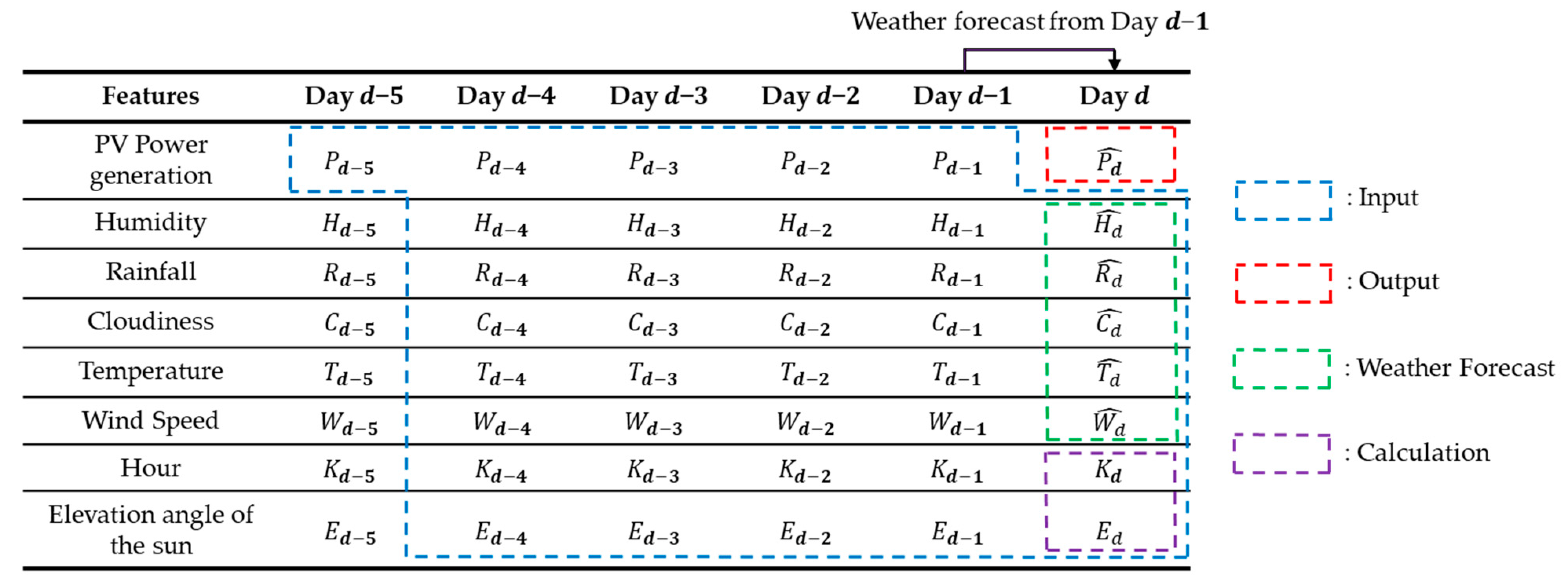
3.3. Testing Phase
Figure 4 shows the inputs and outputs of the testing phase. Similar to the training phase, the input sequences have the same structure as shown in the dotted-blue region. The input sequence of PV power generation is from Day -5 to Day -1, while the other features are from Day -4 to Day . However, the weather data on Day is replaced by the weather data forecasted on Day d-1 as shown in the dotted-green rectangle. This is because the future weather data are not known during the testing phase. The dotted-red rectangle represents the predicted value of .
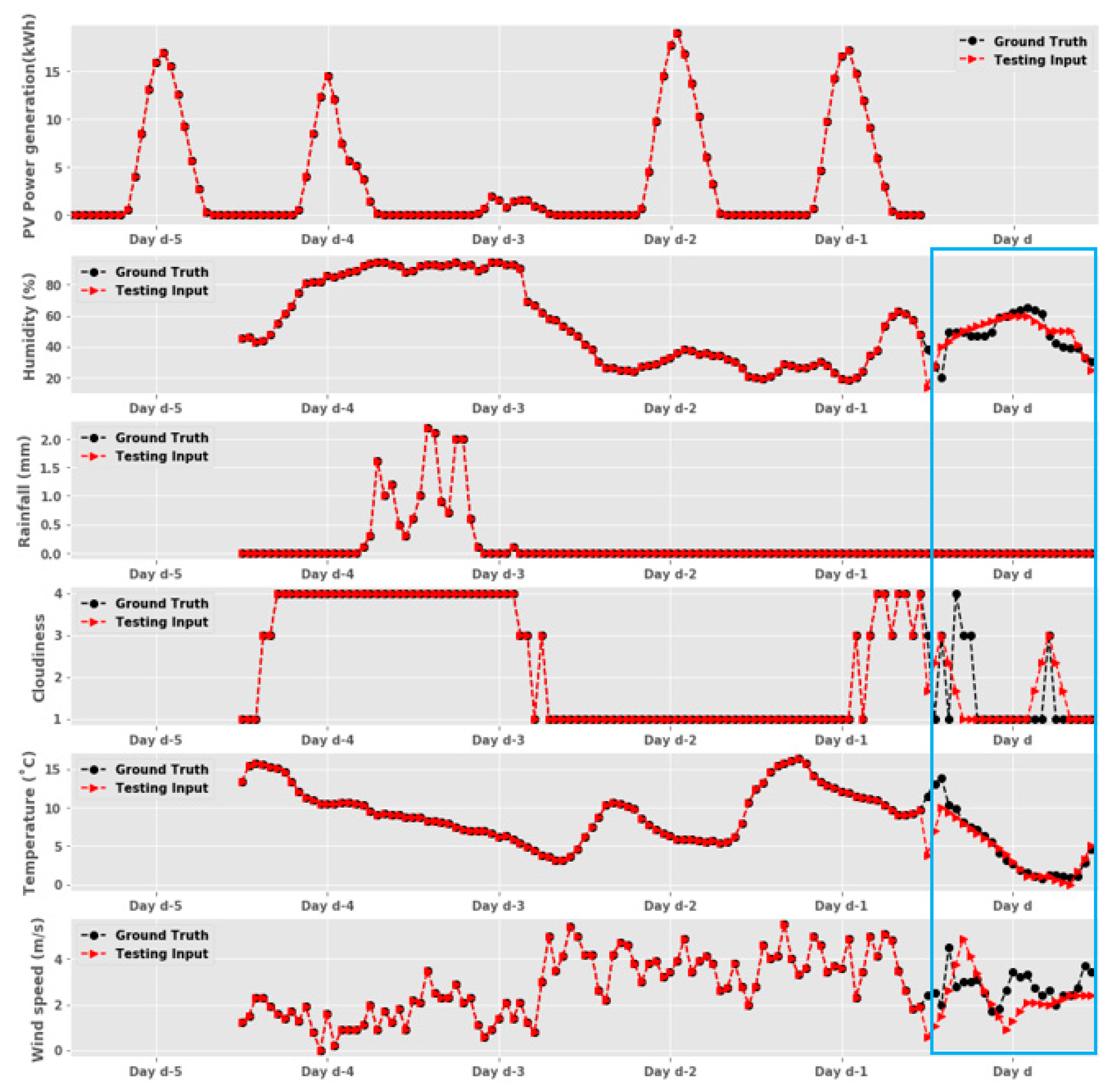
Figure 5 shows an example of the input sequences for the testing phase, assuming that we are trying to forecast Day d. As shown in Figure 5, we use a 5-day sequence of PV power generation from Day -5 to Day -1, where the ground truth and testing input are exactly same. As shown in the blue box in Figure 5, it can be observed that the forecast data replaced with the weather data on Day d are different from the ground truth. Note that the actual values (the black line) are quite different from weather forecasts (the red line) due to the inaccuracy of weather forecasts. Nevertheless, we observe that weather forecast data play an important role in the prediction of PV power generation by giving the model valuable information about the future.
4. Proposed Method
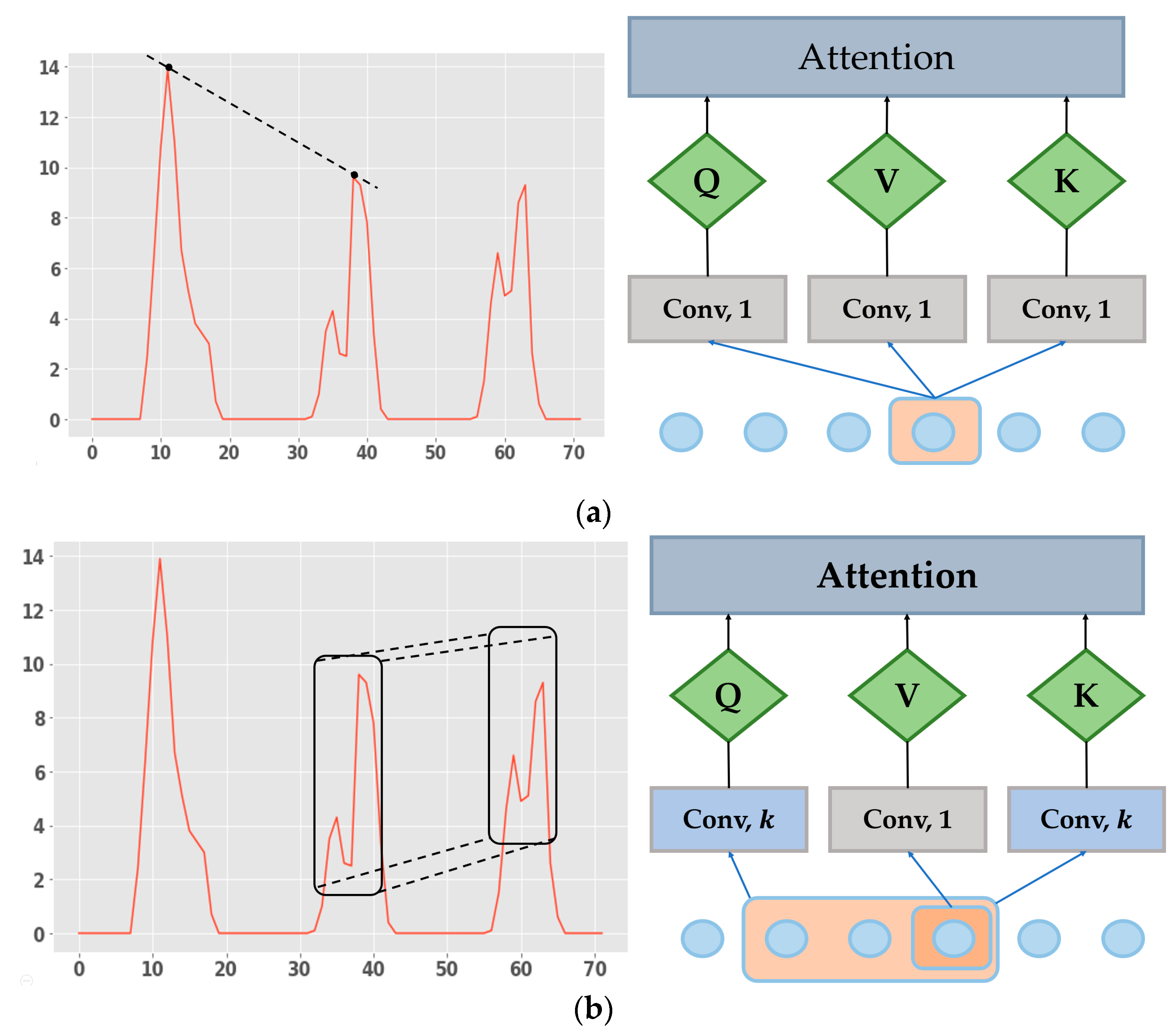
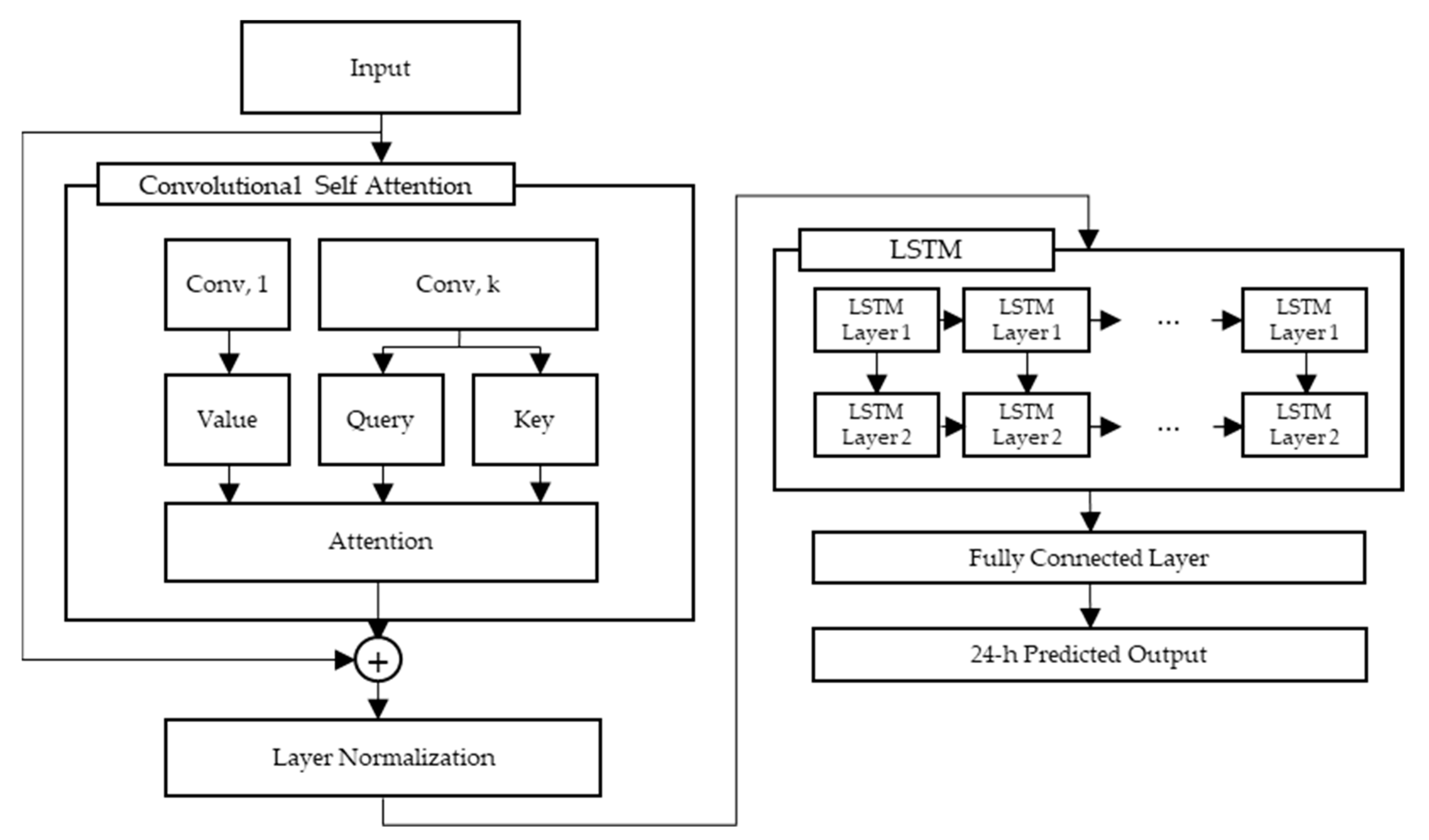
In this paper, we propose the Convolutional Self-Attention LSTM model for day-ahead hourly forecasting of PV power generation. Although LSTM and gradient clipping solve the problem of the RNN, such as the gradient vanishing and expending, it may be possible to fail to utilize all features from long sequence inputs such as data for the past 120 h [36]. Recently, an attention method that emphasizes the important features of long sequence input has been widely used regardless of distance [37,38,39]. In case of LSTM with attention, the amount of lag is an important factor in reducing loss. Additionally, the LSTM with attention shows that it outperforms regular LSTM [40]. On the other hand, some deep learning model may be deteriorated due to the attention technique. The canonical self-attention is one of the attention techniques that cause optimization problems to the model by generating inappropriate keys and queries that do not fit the local context. To address this problem, we apply causal convolution to our model. By applying the causal convolution, we can improve prediction performance by generating queries and keys that are more aware of local context and thus are able to compute their similarities by their local context information, e.g., local shapes, instead of point-wise values [15]. In Figure 6, (a) shows the calculation of the similarity between queries and keys with point-wise values, while (b) shows the calculation of the similarity between queries and keys with the local context.
In addition, we construct a residual connection between the results of convolutional self-attention and input, and also apply the normalization [41]. Then, through the two hidden-layer LSTMs with 256 units passing the fully connected layer, the predicted hourly PV power generation values are generated for the next 1-day (24 h).
5. Experiment
In this paper, we use hourly PV power generation data from 1 October 2017 to 30 March 2020 of the PV power plant in Jebi-ri, Gujeong-myeon, Gangneung-si, Gangwon-do, Korea. We obtain power generation data from a PV power plant in Jebi-ri. The maximum power output of each PV panel used in the Jebi-ri power plant is 150 kW. We also collect hourly weather measurement data for the same period as PV power generation measurement and 3-hourly weather forecast data to be used for testing from the Korean Meteorological Administration (KMA) [42]. Linear interpolation is used to transform the 3-hourly weather forecast data into hourly data. As mentioned in Section 3.1 and Section 3.2, we use the training dataset from October 2017 to February 2020 and the test dataset from 2 March 2020 to 30 March 2020.
5.1. Find k of Convolutional Self-Attention
As shown in Figure 7 in Section 4, we generate queries, keys and values using the convolutional self-attention. The convolution layer with kernel size 1 generates a value, while the convolution layer with kernel size k generates queries and keys. Different values for the size of kernel k may lead to different queries and keys, and thus may have a non-trivial impact on the overall performance of the proposed Convolutional Self-Attention LSTM model. Therefore, we conduct nine sets of experiments varying k from 1 to 9 and measure the MSE (Mean Square Error) of the model to find a suitable k value for the data. Table 2 shows the MSE results according to the k values. Since the results of these experiments show that the lowest MSE is achieved at k = 3, we set the number of k to 3.
5.2. Performance Index
In this paper, Mean Absolute Error (MAE), Mean Absolute Percentage Error (MAPE), Root Mean Squared Error (RMSE) and normalized Mean Absolute Error (nMAE) are used to measure the accuracy of the 1-day prediction. The MAE, MAPE, RMSE, nMAE are defined as:
where represents the number of data, represents the t-th actual PV power generation value, and represents the -th predicted PV power generation value.
5.3. Experimental Results
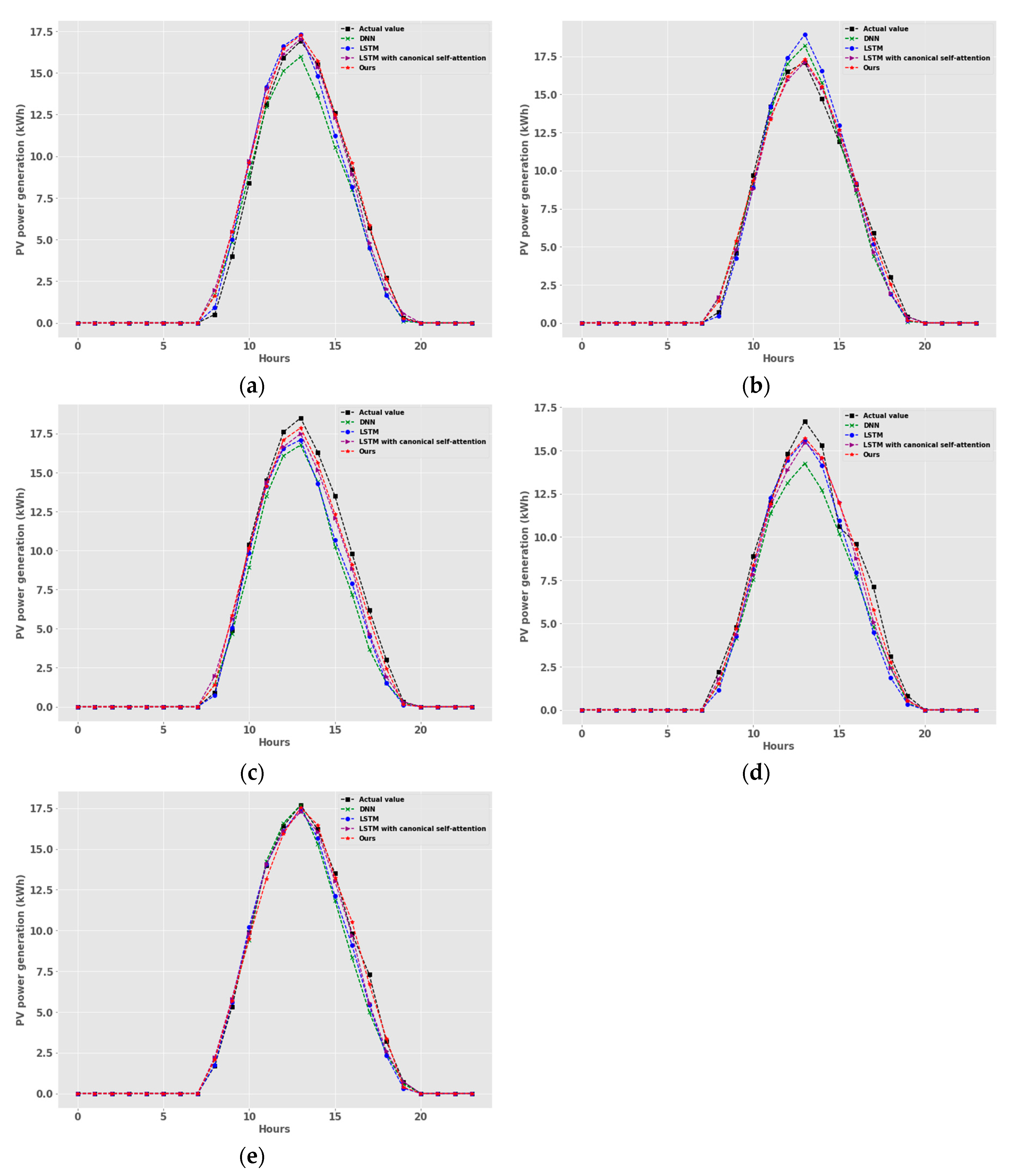
In this section, we assess the efficiency and effectiveness of the proposed Convolutional Self-Attention LSTM model by comparing it against three widely used models, DNN (described in Section 2.1), LSTM (described in Section 2.2), and LSTM with the canonical self-attention. Figure 8 shows the PV power generation forecasting results for each method, i.e., DNN, LSTM, LSTM with the canonical self-attention and our proposed Convolutional Self-Attention LSTM model, respectively. In Figure 8, there are five predicted days by four methods. The proposed Convolutional Self-Attention LSTM model shows a lower forecasting error and consequently higher forecasting accuracy compared with the DNN, LSTM and LSTM with the canonical self-attention model.
The average forecasting errors for the entire test sets are summarized in Table 3. The MAPE of our proposed Convolutional Self-Attention model is lower by 7.7%, 6% and 3.9% compared to the DNN, LSTM and LSTM with the canonical self-attention, respectively.
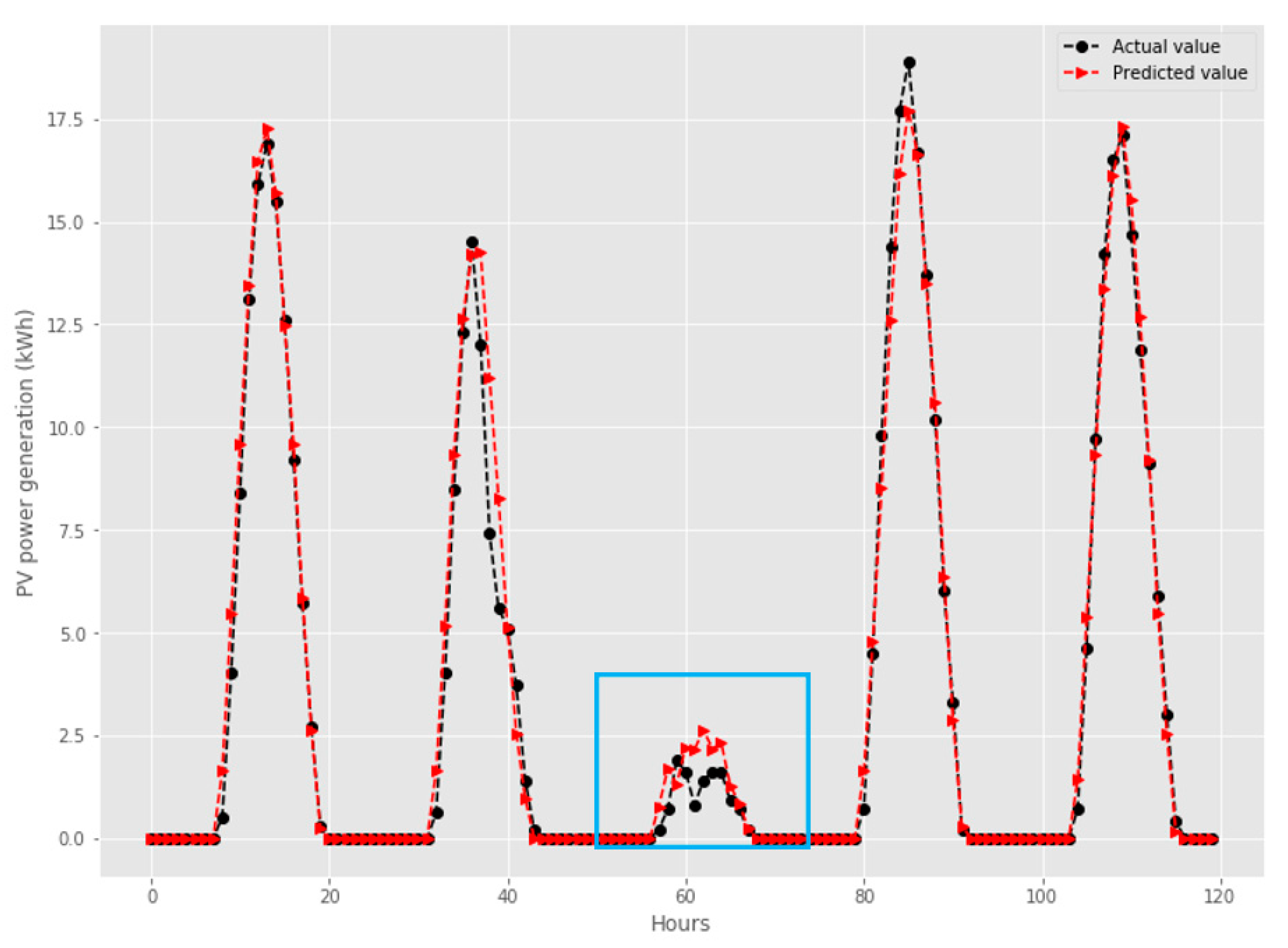
Figure 9 shows the actual PV power generations and predictions for the five consecutive days. In general, the prediction results are similar to actual PV power generation. As shown in the blue box in Figure 9, although PV power generation is lower compared with the other days for several reasons such as poor weather condition, our proposed Convolutional Self-Attention LSTM model predicts the similar pattern on the third day. This means that our proposed model works well even with various weather changes. However, the differences between the red line and the black line are also seen. These errors are mainly due to a lack of data, that is, a pattern that does not exist in the past. Another important factor causing the error is uncertainty in weather forecasts. It can be seen that the uncertainty of weather forecasts can inject incorrect information into a forecast model.
5.4. Effect of Historical and Future Data
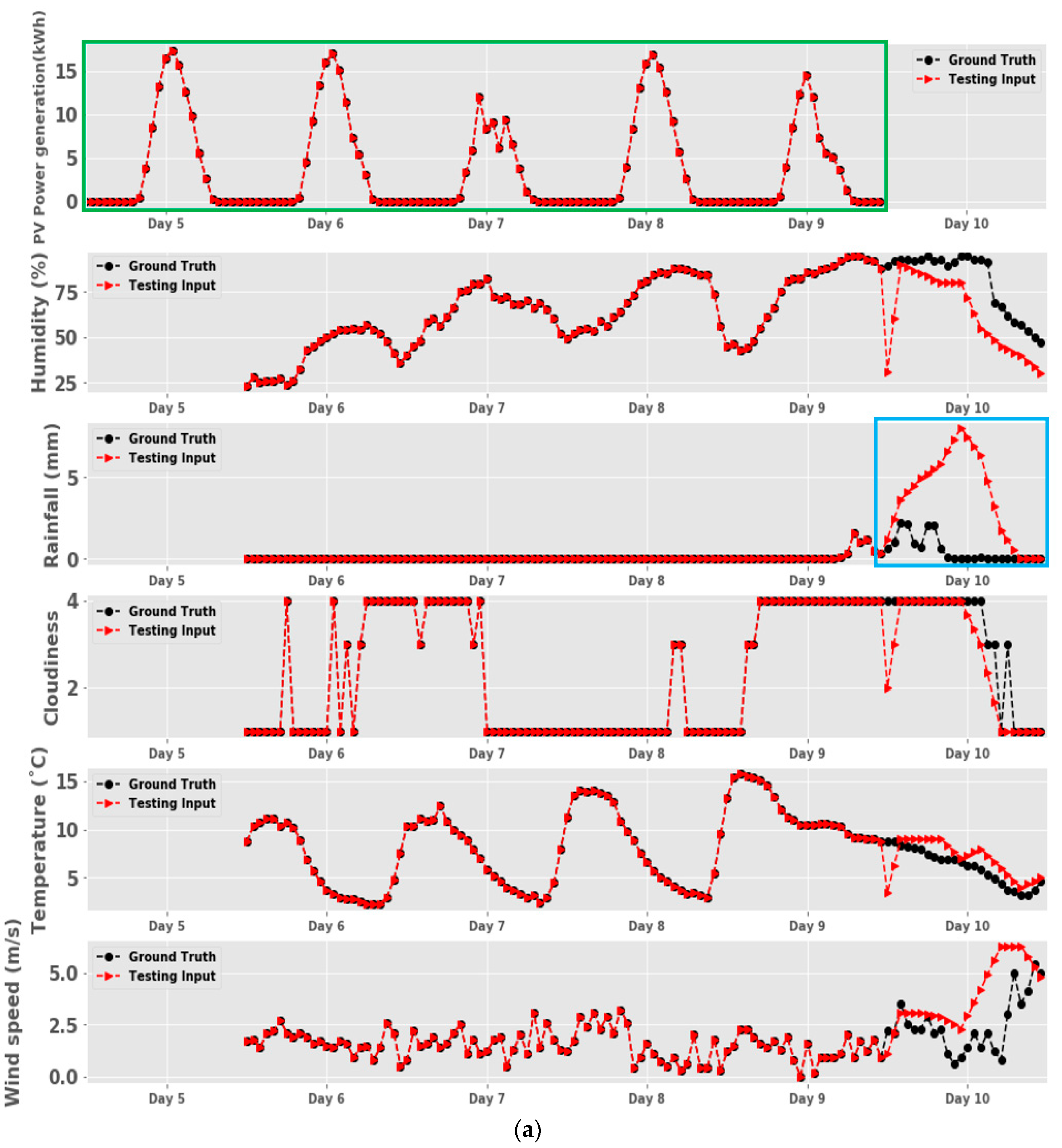
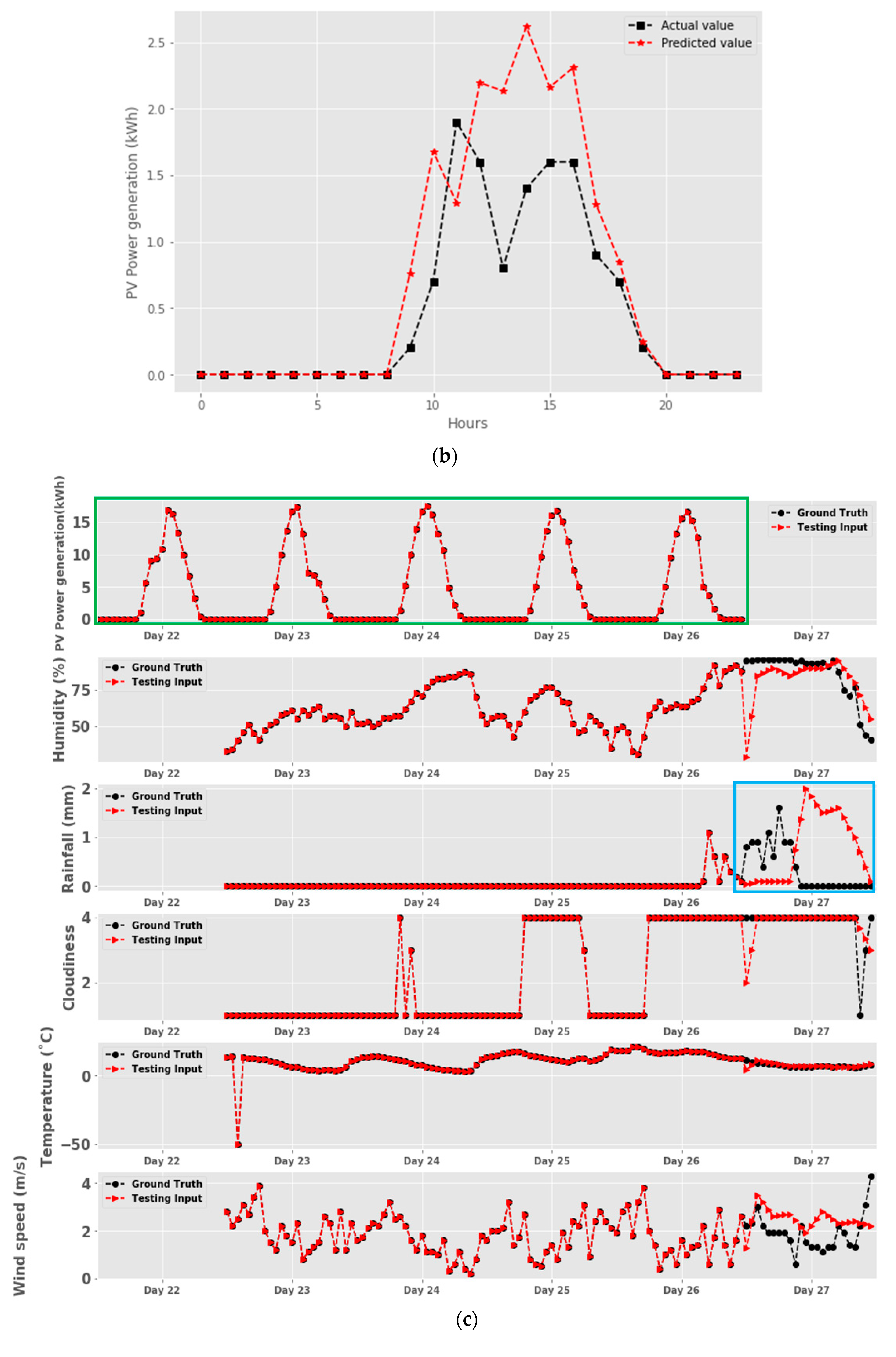
To further analyze the effect of historical and future data, we magnify the blue box in Figure 9 as shown in Figure 10. The historical and future data for predicting the PV power generation on the third day is shown in Figure 10a and its result is depicted in Figure 10b. Note that Figure 10b is the same as the blue box in Figure 9.
As shown in the green box in Figure 10a, the curve of PV power generation shows some lot fluctuations, which produce a high information gain that is helpful for accurate prediction. In addition, as shown in the blue box in Figure 10a, the weather forecast (the red line) predicted rain and the precipitation of 8 mm on day 10. Based on this information, the proposed model can predict an accurate amount of PV power generation as shown in Figure 10b by capturing historical features and also acquiring helpful information from weather forecasts.
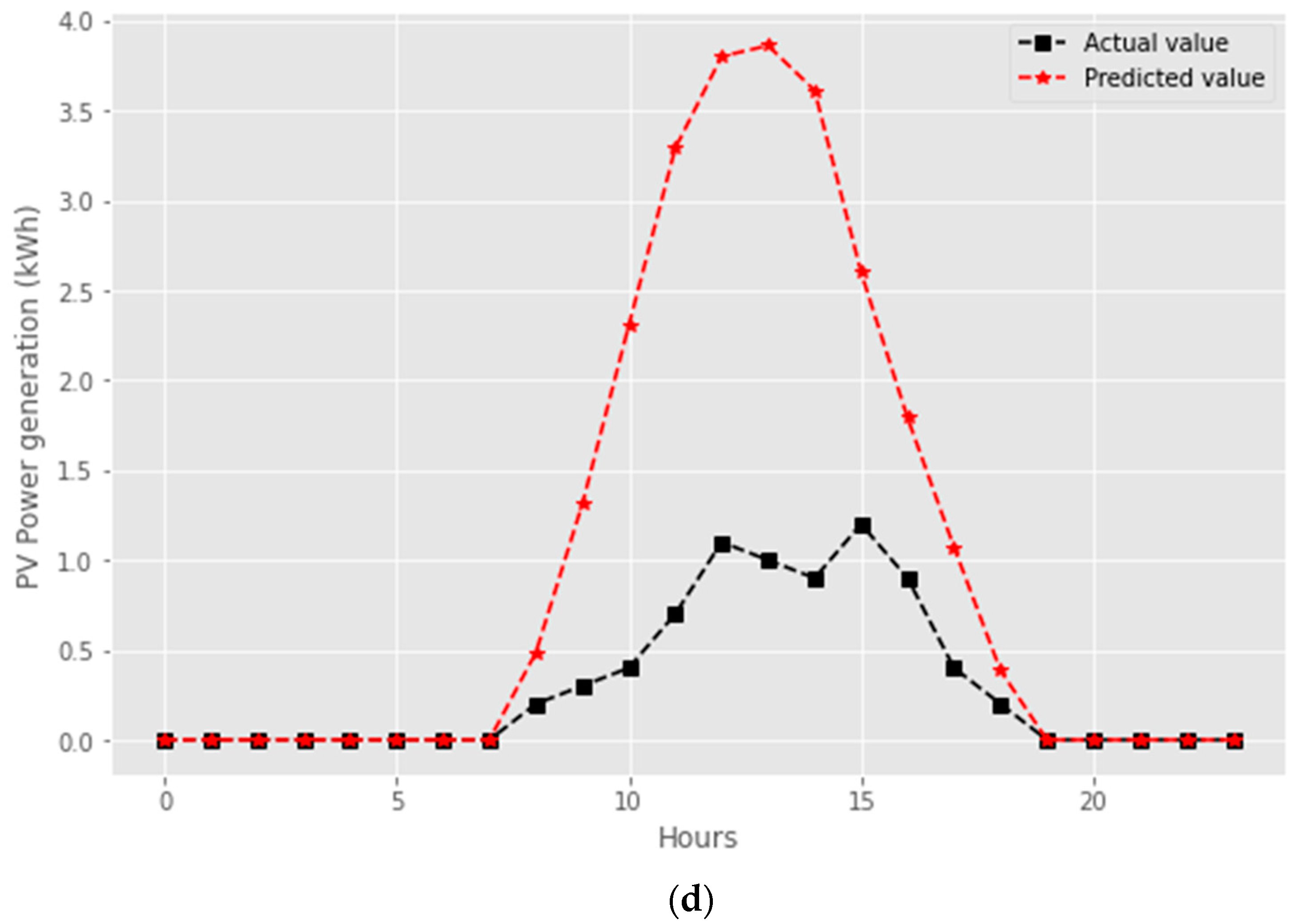
On the other hand, Figure 10d shows an inaccurate case. In this case, the curve of PV power generation shows consistent patterns for 5 days, which generate lower information for predicting a sudden decline in PV power generation. This low information gain can have a negative impact on a prediction model. In addition, because the weather forecast in the blue box in Figure 10c is inaccurate, the proposed model can only predict a fairly different amount of PV power generation than the actual PV power generation as shown in the red line in Figure 10d.
5.5. NSW Electricity Load Data
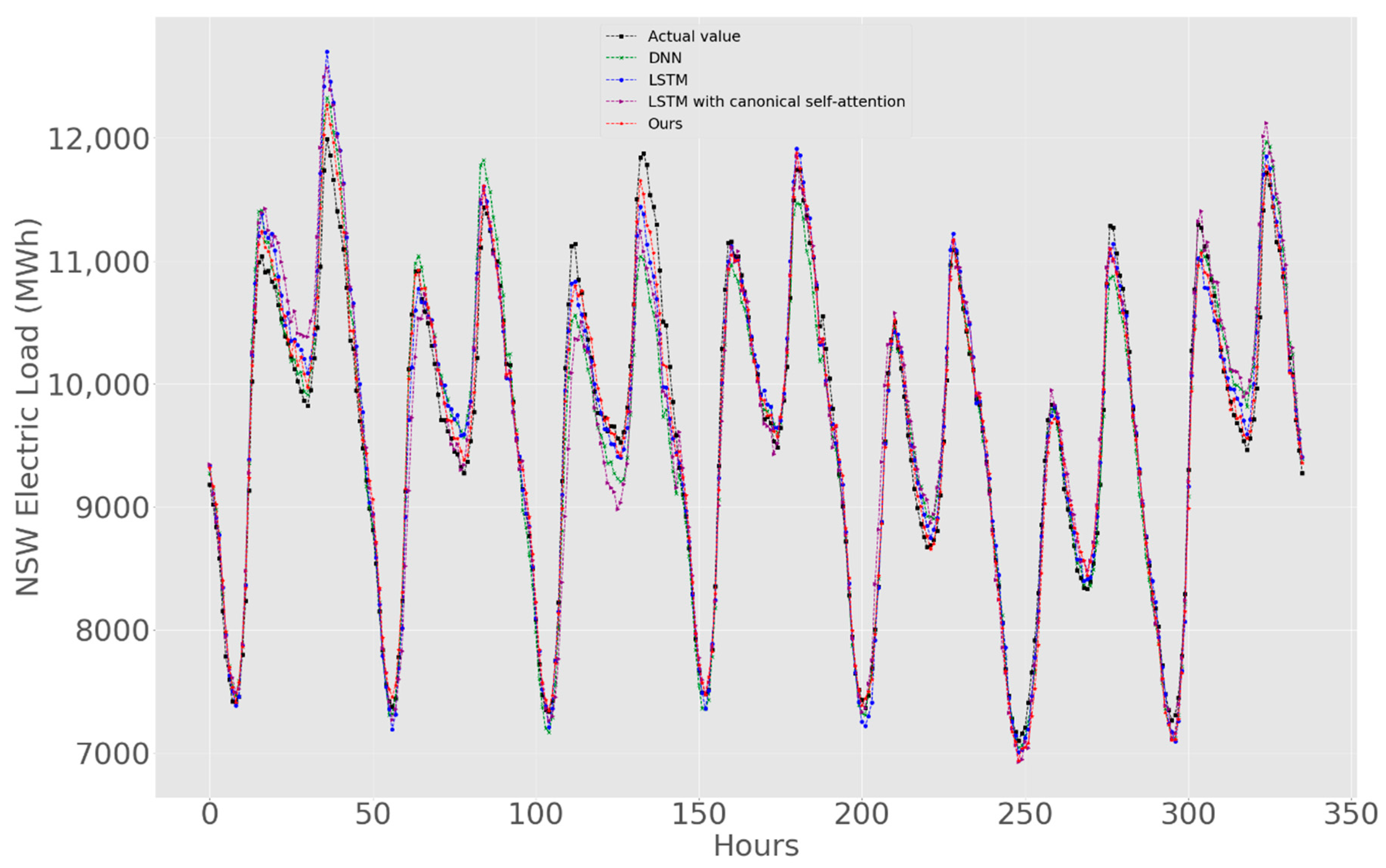
In order to validate our proposed model, we conduct an experiment using another type of time series data such as the NSW (New South Wales) electricity load data [43]. The NSW electricity load data include hour, dry bulb temperature, dew point temperature, wet bulb temperature, humidity, electricity price and system load. It is constructed by measuring every 30 min from 1 January 2006 to 1 January 2011. For NSW data, since the future data, such as weather forecast, is unknown, we use only the past 5-day data as input to predict the future 1-day electricity load. Figure 11 shows the forecasting results for seven consecutive days. As shown in Figure 11, the proposed Convolutional Self-Attention LSTM model predicts a closer matching pattern to the actual electricity load than other methods. The MAPE of the proposed model is much lower by 32%, 17% and 44% compared to the DNN, LSTM and LSTM with the canonical self-attention, respectively. This result indicates that the proposed Convolutional Self-Attention LSTM model predicts not only PV power generations but also power consumptions.
6. Conclusions
In this paper, we propose the Convolutional Self-Attention LSTM model for forecasting day-ahead hourly PV power generations by applying the convolution self-attention technique. Unlike previous methods using the canonical self-attention, our proposed method is able to generate queries and keys that are more aware of local context and thus are able to improve prediction performance by computing their similarities with their local context information. In addition to the convolution self-attention, our model uses both historical and future data by replacing the past weather data with the future weather forecast data during the testing phase.
We compare our proposed model with existing methods: the DNN-based model, LSTM-based model and LSTM with the canonical self-attention. Extensive experiments using the real world datasets show that the MAPE of the proposed Convolutional Self-Attention LSTM model is much lower by 7.7%, 6%, 3.9% compared to the DNN, LSTM and LSTM with the canonical self-attention, respectively. In addition, in order to validate the applicability of the proposed model, we conduct another set of experiments on forecasting power consumptions using the NSW electricity load data. In these experiments, we observed that the proposed Convolutional Self-Attention LSTM model has reduced error rates by 32%, 17% and 44% for MAPE compared to the DNN, LSTM and LSTM with the canonical self-attention-based models, respectively.
For future work, we plan to augment our method with harsh conditions where the daily PV power generation is not in the form of a parabola and its deviation is quite severe due to poor weather conditions. We also plan to extend our model to predict various forecast horizons ranging from 5 min to a half-hour.
Author Contributions
D.Y. designed the Convolutional Self-Attention LSTM based model, conducted the experiments, and prepared the manuscript as the first author. W.C. and M.K. led the project and research. L.L. assisted with the research and contributed to writing and revising the manuscript. All authors discussed the results of the experiments and were involved in preparing the manuscript. All authors have read and agreed to the published version of the manuscript.
Funding
This research was funded by Korea Electric Power Corporation (Grant number: R18XA01) and the Ministry of Trade, Industry and Energy (MOTIE), Korea Institute for Advancement of Technology (KIAT) (No. P0006132).
Acknowledgments
This research was supported by Korea Electric Power Corporation (Grant number: R18XA01). This research was partially supported by the Ministry of Trade, Industry and Energy (MOTIE), Korea Institute for Advancement of Technology (KIAT) through the Encouragement Program for the Industries of Economic Cooperation Region (No: P0006132).
Conflicts of Interest
The authors declare no conflict of interest.
References
- Nosratabadi, S.M.; Hooshmand, R.-A.; Gholipour, E. A comprehensive review on microgrid and virtual power plant concepts employed for distributed energy resources scheduling in power systems. Renew. Sustain. Energy Rev. 2017, 67, 341–363. [Google Scholar] [CrossRef]
- Hatziargyriou, N.; Asano, H.; Marnay, R.I.C. Microgrids: An overview of ongoing research development and demonstration projects. IEEE Power Energy Mag. 2017, 5, 78–94. [Google Scholar] [CrossRef]
- Awerbuch, S.; Preston, A. The Virtual Utility: Accounting, Technology & Competitive Aspects of the Emerging Industry; Springer Science & Business Media: New York, NY, USA, 1997. [Google Scholar]
- Pudjianto, D.; Ramsay, C.; Strbac, G. Virtual power plant and system integration of distributed energy resources. In IET Renewable Power Generation; Institution of Engineering and Technology: London, UK, 2007; Volume 1, pp. 10–16. [Google Scholar]
- Su, W.; Wang, J. Energy management systems in micrgrid operations. Electr. J. 2012, 25, 45–60. [Google Scholar] [CrossRef]
- Moutis, P.; Hatziargyriou, N.D. Decision trees aided scheduling for firm power capacity provision by virtual power plants. Int. J. Electr. Power Energy Syst. 2014, 63, 730–739. [Google Scholar] [CrossRef]
- Sharma, N.; Sharma, P.; Irwin, D.E.; Shenoy, P.J. Predicting solar generation from weather forecasts using machine learning. In Proceedings of the 2nd IEEE International Conference on Smart Grid Communications (SmartGridComm), Brussels, Belgium, 17–20 October 2011; pp. 17–20. [Google Scholar]
- Tao, C.; Shanxu, D.; Changsong, C. Forecasting power output for grid-connected PV power system without using solar radiation measurement. In Proceedings of the 2nd IEEE International Symposium on Power Electronics for Distributed Generation Systems, Hefei, China, 16–18 June 2010. [Google Scholar]
- Das, U.K.; Tey, K.S.; Seyedmahmoudian, M.; Mekhilef, S.; Idris, M.Y.I.; Van Deventer, W.; Stojcevski, A. Forecasting of PV power generation and model optimization: A review. Renew. Sustain. Energy Rev. 2018, 81, 912–928. [Google Scholar] [CrossRef]
- Jeong, J.; Kim, H. Multi-Site Photovoltaic Forecasting Exploiting Space-Time Convolutional Neural Network. Energies 2019, 12, 4490. [Google Scholar] [CrossRef] [Green Version]
- Choi, S.; Hur, J. An Ensemble Learner-Based Bagging Model Using Past Output Data for Photovoltaic Forecasting. Energies 2020, 13, 1438. [Google Scholar] [CrossRef] [Green Version]
- Aprillia, H.; Yang, H.-T.; Huang, C.-M. Short-Term Photovoltaic Power Forecasting Using a Convolutional Neural Network–Salp Swarm Algorithm. Energies 2020, 13, 1879. [Google Scholar] [CrossRef]
- Ding, M.; Wang, L.; Bi, R. An ANN-based Approach for Forecasting the Power Output of PV System. Procedia Environ. Sci. 2011, 11, 1308–1315. [Google Scholar] [CrossRef] [Green Version]
- Chen, C.; Duan, S.; Cai, T.; Liu, B. Online 24-h solar power forecasting based on weather type classification using artificial neural network. Sol. Energy 2011, 85, 2856–2870. [Google Scholar] [CrossRef]
- Li, S.; Jin, X.; Xuan, Y.; Zhou, X.; Chen, W.; Wang, Y.X.; Yan, X. Enhancing the locality and breaking the memory bottleneck of transformer on time series forecasting. In Advances in Neural Information Processing Systems (NeurIPS); Association for Computing Machinery: Vancouver, BC, Canana, 2019; Volume 32, pp. 5244–5254. [Google Scholar]
- Mellit, A.; Massi Pavan, A.; Ogliari, E.; Leva, S.; Lughi, V. Advanced Methods for PV Output Power Forecasting: A Review. Appl. Sci. 2020, 10, 487. [Google Scholar] [CrossRef] [Green Version]
- Huang, R.; Huang, T.; Gadh, R.; Li, N. Solar generation prediction using the ARMA model in a laboratory-level micro-grid. In Proceedings of the third International Conference on Smart Grid Communications (SmartGridComm), Tainan, Taiwan, 5–8 November 2012; pp. 528–533. [Google Scholar]
- Li, Y.; Su, Y.; Shu, L. An ARMAX Model for Forecasting The Power Output of A Grid Connected PV System. Renew. Energy 2014, 66, 78–89. [Google Scholar] [CrossRef]
- Zeng, J.; Qiao, W. Short-term solar power prediction using a support vector machine. Renew. Energy 2013, 52, 118–127. [Google Scholar] [CrossRef]
- Mellit, A.; Massi Pavan, A.; Lughi, V. Short-term forecasting of power production in a large-scale PV plant. Sol. Energy 2014, 105, 401–413. [Google Scholar] [CrossRef]
- Fernandez-Jimenez, L.A.; Munoz-Jimenez, A.; Falces, A.; Mendoza-Villena, M.; Garcia-Garrido, E.; Lara-Santillan, P.M.; Zorzano-Santamaria, P.J. Short-term power forecasting system for PV plants. Renew. Energy 2012, 44, 311–317. [Google Scholar] [CrossRef]
- Son, J.; Park, Y.; Lee, J.; Kim, H. Sensorless PV power forecasting in grid-connected buildings through deep learning. Sensors 2018, 18, 2529. [Google Scholar] [CrossRef] [PubMed] [Green Version]
- Abdel-Nasser, M.; Mahmoud, K. Accurate PV power forecasting models using deep LSTM-RNN. Neural Comput. Appl. 2017, 31, 2727–2740. [Google Scholar] [CrossRef]
- Qing, X.; Niu, Y. Hourly day-ahead solar irradiance prediction using weather forecasts by LSTM. Energy 2018, 148, 461–468. [Google Scholar] [CrossRef]
- Huang, C.-J.; Kuo, P.-H. Multiple-input deep convolutional neural network model for short-term photovoltaic power forecasting. IEEE Access 2019, 7, 74822–74834. [Google Scholar] [CrossRef]
- Chang, G.W.; Lu, H.-J. Integrating Gray Data Preprocessor and Deep Belief Network for Day-Ahead PV Power Output Forecast. IEEE Trans. Sustain. Energy 2018, 11, 185–194. [Google Scholar] [CrossRef]
- Haneul, E.; Son, Y.; Choi, S. Feature-Selective Ensemble Learning-Based Long-Term Regional PV Generation Forecasting. IEEE Access 2020, 8, 54620–54630. [Google Scholar]
- Bouzerdoum, M.; Mellit, A.; Massi Pavan, A. A hybrid model (SARIMA-SVM) for short-term power forecasting of a small-scale grid-connected PV plant. Sol. Energy 2013, 98, 226–235. [Google Scholar] [CrossRef]
- Behera, M.K.; Majumder, I.; Nayak, N. Solar PV power forecasting using optimized modified extreme learning machine technique. Eng. Sci. Technol. Int. J. 2019, 21, 428–438. [Google Scholar]
- Dolara, A.; Grimaccia, F.; Leva, S.; Mussetta, M.; Ogliari, E. A physical hybrid artificial neural network for short term forecasting of PV plant power output. Energies 2015, 8, 1138–1153. [Google Scholar] [CrossRef] [Green Version]
- Maddix, D.C.; Wang, Y.; Smola, A. Deep factors with Gaussian processes for forecasting. arXiv 2018, arXiv:1812.00098. [Google Scholar]
- Lai, G.; Chang, W.-C.; Yang, Y.; Liu, H. Modeling long-and short-term temporal patterns with deep neural networks. In Proceedings of the 41st International ACM SIGIR Conference on Research & Development in Information Retrieval, Ann Arbor, MI, USA, 8–12 July 2018; pp. 95–104. [Google Scholar]
- Pascanu, R.; Mikolov, T.; Bengio, Y. On the difficulty of training recurrent neural networks. In Proceedings of the International Conference on Machine Learning, Atlanta, GA, USA, 16–21 June 2013; pp. 1310–1318. [Google Scholar]
- Hochreiter, S.; Schmidhuber, J. Long short-term memory. Neural Comput. 1997, 9, 1735–1780. [Google Scholar] [CrossRef]
- Khandelwal, U.; He, H.; Qi, P.; Jurafsky, D. Sharp nearby, fuzzy far away: How neural language models use context. arXiv 2018, arXiv:1805.04623. [Google Scholar]
- Meeus, J. Astronomical Algorithms, 2nd ed.; William-Bell: Virginia, WV, USA, 1998. [Google Scholar]
- Zhou, H.; Zhang, Y.; Yang, L.; Liu, Q.; Yan, K.; Du, Y. Short-term PV power forecasting based on long short term memory neural network and attention mechanism. IEEE Access 2019, 7, 78063–78074. [Google Scholar] [CrossRef]
- Wang, S.; Wang, X.; Wang, S.; Wang, D. Bi-directional long short-term memory method based on attention mechanism and rolling update for short-term load forecasting. Int. J. Electr. Power Energy Syst. 2019, 109, 470–479. [Google Scholar] [CrossRef]
- Hao, S.; Lee, D.-H.; Zhao, D. Sequence to sequence learning with attention mechanism for short-term passenger flow prediction in large-scale metro system. Transp. Res. Part C Emerg. Technol. 2019, 107, 287–300. [Google Scholar] [CrossRef]
- Hollis, T.; Viscardi, A.; Yi, S.E. A comparison of LSTMs and attention mechanisms for forecasting financial time series. arXiv 2018, arXiv:1812.07699. [Google Scholar]
- Ba, J.L.; Kiros, J.R.; Hinton, G.E. Layer normalization. arXiv 2016, arXiv:1607.06450. [Google Scholar]
- Korea Meteorological Administration. Climate of Korea. Available online: https://web.kma.go.kr/eng/biz/climate_01.jsp (accessed on 3 April 2020).
- Australian Energy Market Operator (AEMO). Available online: http://www.aemo.com.au (accessed on 3 June 2020).
Figure 1.
Deep Neural Network (DNN) based model architecture.

Figure 2.
Long Short-Term Memory (LSTM)-based model: (a) the inner of the LSTM; (b) the LSTM-based model architecture.
Figure 2.
Long Short-Term Memory (LSTM)-based model: (a) the inner of the LSTM; (b) the LSTM-based model architecture.

Figure 3.
Inputs and outputs at the training phase.

Figure 4.
Inputs and outputs at the testing phase.

Figure 5.
Example of Photovoltaic (PV) power generation and weather data used for the testing phase.
Figure 5.
Example of Photovoltaic (PV) power generation and weather data used for the testing phase.

Figure 6.
Comparison of canonical self-attention and convolutional self-attention techniques: (a) canonical self-attention; (b) convolutional self-attention, confirming the observation in [15], with slight variation.
Figure 6.
Comparison of canonical self-attention and convolutional self-attention techniques: (a) canonical self-attention; (b) convolutional self-attention, confirming the observation in [15], with slight variation.

Figure 7.
Architecture of Convolutional Self-Attention Long Short-Term Memory (LSTM) model.

Figure 8.
Forecasting results: (a) forecasting result on 8 March 2020; (b) forecasting result on 12 March 2020; (c) forecasting result on 14 March 2020; (d) forecasting result on 28 March 2020; (e) forecasting result on 30 March 2020.
Figure 8.
Forecasting results: (a) forecasting result on 8 March 2020; (b) forecasting result on 12 March 2020; (c) forecasting result on 14 March 2020; (d) forecasting result on 28 March 2020; (e) forecasting result on 30 March 2020.

Figure 9.
Forecasting result from 8 March 2020 to 12 March 2020.

Figure 10.
Forecasting results according to the uncertainty of historical and future data: (a) historical and future data for 10 March 2020; (b) forecasting result on 10 March 2020; (c) historical and future data on 27 March 2020; (d) forecasting result for 27 March 2020.
Figure 10.
Forecasting results according to the uncertainty of historical and future data: (a) historical and future data for 10 March 2020; (b) forecasting result on 10 March 2020; (c) historical and future data on 27 March 2020; (d) forecasting result for 27 March 2020.


Figure 11.
Forecast results of NSW (New South Wales) electricity load.


Table 1.
Notation of features for each day.
| Features | Day d-5 | Day d-4 | Day d-3 | Day d-2 | Day d-1 | Day d |
|---|---|---|---|---|---|---|
| PV Power Generation | ||||||
| Humidity | ||||||
| Rainfall | ||||||
| Cloudiness | ||||||
| Temperature | ||||||
| Wind Speed | ||||||
| Hour | ||||||
| Elevation Angle of the Sun |
Table 2.
MSE (Mean Square Error) by k values. (The value in bold is the minimum value.).
| k | 1 | 2 | 3 | 4 | 5 | 6 | 7 | 8 | 9 |
|---|---|---|---|---|---|---|---|---|---|
| MSE | 0.0038 | 0.0036 | 0.0035 | 0.0039 | 0.0040 | 0.0037 | 0.0039 | 0.0039 | 0.0039 |
Table 3.
Comparison of PV power generation forecasting performance. (The value in bold in each column is the minimum value.).
Table 3.
Comparison of PV power generation forecasting performance. (The value in bold in each column is the minimum value.).
| Method | MAPE (%) | MAE (kWh) | RMSE | nMAE |
|---|---|---|---|---|
| DNN | 26.25 | 0.66 | 1.36 | 0.17 |
| LSTM | 25.77 | 0.59 | 1.32 | 0.15 |
| LSTM with canonical self-attention | 25.21 | 0.63 | 1.30 | 0.16 |
| Ours | 24.22 | 0.57 | 1.24 | 0.15 |
© 2020 by the authors. Licensee MDPI, Basel, Switzerland. This article is an open access article distributed under the terms and conditions of the Creative Commons Attribution (CC BY) license (http://creativecommons.org/licenses/by/4.0/).
Share and Cite
MDPI and ACS Style
Yu, D.; Choi, W.; Kim, M.; Liu, L. Forecasting Day-Ahead Hourly Photovoltaic Power Generation Using Convolutional Self-Attention Based Long Short-Term Memory. Energies 2020, 13, 4017. https://0-doi-org.brum.beds.ac.uk/10.3390/en13154017
AMA Style
Yu D, Choi W, Kim M, Liu L. Forecasting Day-Ahead Hourly Photovoltaic Power Generation Using Convolutional Self-Attention Based Long Short-Term Memory. Energies. 2020; 13(15):4017. https://0-doi-org.brum.beds.ac.uk/10.3390/en13154017
Chicago/Turabian StyleYu, Dukhwan, Wonik Choi, Myoungsoo Kim, and Ling Liu. 2020. "Forecasting Day-Ahead Hourly Photovoltaic Power Generation Using Convolutional Self-Attention Based Long Short-Term Memory" Energies 13, no. 15: 4017. https://0-doi-org.brum.beds.ac.uk/10.3390/en13154017
Note that from the first issue of 2016, this journal uses article numbers instead of page numbers. See further details here.