
CO2 Intensities and Primary Energy Factors in the Future European Electricity System


Department of Economics, Faculty of Economics and Business Administration, Ghent University, 9000 Ghent, Belgium
Energies 2021, 14(8), 2165; https://0-doi-org.brum.beds.ac.uk/10.3390/en14082165
Submission received: 7 March 2021
/
Revised: 31 March 2021
/
Accepted: 6 April 2021
/
Published: 13 April 2021
(This article belongs to the Special Issue Electrical Engineering for Sustainable and Renewable Energy)
Abstract
:The European Union strives for sharp reductions in both CO2 emissions as well as primary energy use. Electricity consuming technologies are becoming increasingly important in this context, due to the ongoing electrification of transport and heating services. To correctly evaluate these technologies, conversion factors are needed—namely CO2 intensities and primary energy factors (PEFs). However, this evaluation is hindered by the unavailability of a high-quality database of conversion factor values. Ideally, such a database has a broad geographical scope, a high temporal resolution and considers cross-country exchanges of electricity as well as future evolutions in the electricity mix. In this paper, a state-of-the-art unit commitment economic dispatch model of the European electricity system is developed and a flow-tracing technique is innovatively applied to future scenarios (2025–2040)—to generate such a database and make it publicly available. Important dynamics are revealed, including an overall decrease in conversion factor values as well as considerable temporal variability at both the seasonal and hourly level. Furthermore, the importance of taking into account imports and carefully considering the calculation methodology for PEFs are both confirmed. Future estimates of the CO2 emissions and primary energy use associated with individual electrical loads can be meaningfully improved by taking into account these dynamics.
1. Introduction
The European Union (EU) strives for sharp reductions in both its primary energy use and CO2 emissions, as formalized in the flagship 2030 policy targets [1]. Electricity-consuming technologies play an increasingly important role in this regard, due to the ongoing electrification of transport and heating services. This underscores the need to properly evaluate the CO2 emissions and primary energy use of individual electrical loads—for which conversion factors such as CO2 intensities and primary energy factors (PEFs) are needed. For example, the CO2 emissions associated with charging an electric vehicle (EV) can be estimated using a CO2 intensity (expressed in kg/MWh), and the primary energy use associated with an electric heat pump (HP) can be estimated using a PEF (expressed in MWhp/MWhe). MWhe stands for electrical energy while MWhp stands for primary energy, which is consumed in the electricity generation process—typically by burning fuels, which contain potential energy in the form of chemical bonds. Both conversion factors reflect how the consumed electricity was produced.
The calculation and use of conversion factors is a contentious issue, because they can affect the outcome of a variety of analyses. For example, previous work has indicated that the CO2 emissions savings realized by substituting fossil-fueled vehicles with EVs are largely dependent on the assumed CO2 intensity of the electricity used to charge the EVs [2,3]. It is even shown in this work that differences in the assumed CO2 intensity can lead to completely opposing conclusions with respect to the merits of EVs. Similarly, PEFs influence the degree to which the installation of a HP or solar panels results in the reduction of a building’s primary energy use [4,5]. From the perspective of HPs, a lower PEF is beneficial because it means the consumed electricity is associated with a lower amount of primary energy use. Meanwhile, a higher PEF is beneficial for solar panels, because their electricity production is typically multiplied by the PEF to calculate the reduction in a building’s primary energy use. This assumes that the electricity production by the solar panels displaces electricity production that would have otherwise taken place in the (national) electricity system [6,7,8]. Due to its interactions with both HPs and solar panels, PEFs can also determine whether or not a building qualifies as a nearly zero energy building [9].
Across the academic literature, conversion factors are used in a variety of applications. Most frequently, they are used to evaluate various building renovation scenarios or design options for newly-built projects [10,11,12,13,14,15,16,17]. In these cases, the primary energy use and CO2 emissions are calculated for certain renovation measures or building designs. Some of the other applications for which conversion factors are used in the literature include an assessment of the CO2 emissions reduction potential of energy communities [7], the design of control strategies for flexible electricity demand [18], and even an assessment of the benefits of electrifying offshore oil platforms [19].
Crucially, conversion factors are subject to a number of methodological characteristics. First of all, their temporal resolution can reflect the electricity mix across an entire year, or across a single season, month, or hour. Secondly, conversion factors can either be based on electricity generation that has taken place in the past (referring to a particular historical year), or on an estimation of what the electricity production mix will look like at some point in the future. This can be referred to as a conversion factor’s temporal scope. Thirdly, some conversion factors only consider the electricity production within a given country, while others take into account the electricity imported from other countries as well. For each of these three methodological characteristics, the recent literature indicates that “inferior” approaches are still being widely used.
In terms of temporal resolutions, many recent studies still use yearly conversion factors [8,20,21,22,23], even though it has been widely recognized elsewhere that it is often better to use monthly or even hourly conversion factors [24,25,26,27,28,29]. By using higher resolutions, temporal changes in the electricity mix are better taken into account. For example, it may be important to consider the seasonal fluctuation of a PEF when the primary energy use associated with a HP is calculated, given the fact that both the PEF itself and the electricity consumption of the HP can vary significantly from season to season. Similarly, it may be important to consider the hourly fluctuations of a CO2 intensity when the CO2 emissions associated with charging an EV (during particular hours of the day) are being calculated. Yearly conversion factors ignore these important temporal variations, leading to inaccurate results [24,25,26,27,28,29].
In terms of temporal scopes, it is clear that retrospective conversion factors—which are based on the electricity mix as observed at some point in the past—are still dominant in the literature [24,30,31,32,33]. In these cases, results are at risk of quickly becoming outdated, given the fact that the electricity mix is rapidly changing across Europe. For example, calculating the primary energy use associated with a HP on the basis of a PEF that refers to a country’s electricity mix several years ago could be problematic, especially if the results are meant to inform future policies. A few recent studies have therefore opted to use prospective conversion factors, anticipating future changes in the electricity mix [8,34,35,36,37]. Whether it is the primary energy use associated with a HP that is being estimated, the CO2 emissions associated with charging EVs, or any other application of conversion factors, prospective values can be considered a superior option if the goal is to inform policies in a forward-looking way.
In line with the frequent use of yearly temporal resolutions and retrospective conversion factors, the handling of imported electricity in the calculation of conversion factors is another methodological issue that is found in the literature. Many recent studies still use conversion factors that do not consider the imports of electricity from neighboring countries [4,5,28,38,39,40,41,42]. Whenever a country covers a large share of its electricity consumption with imports from other countries, taking these imports into account can be of considerable importance. For example, the CO2 emissions associated with charging an EV in Belgium may not only be determined by the electricity mix in Belgium, but also by the electricity mix of the countries it imports from (e.g., France and Germany).
Increasing the use of hourly and prospective conversion factors, which also take into account imports, could improve the future research endeavors in which the primary energy use and CO2 emissions associated with a variety of electrical loads is calculated. Furthermore, it could thereby also lead to improvements in the policies that are aimed at realizing reductions on those two fronts. However, the thorough calculation of such conversion factors constitutes a considerable challenge, because it requires a sophisticated modelling exercise—in which the interconnected European electricity system of the future is simulated in a rigorous way. Because of this, a publicly available and up-to-date database of the described conversion factors has so far remained unavailable—and this has been recognized as a barrier to research in a variety of recent studies [4,8,37,43,44], indicating a gap in the literature.
The present paper addresses this gap by developing and using a state-of-the-art model of the future European electricity system and innovatively applying a flow-tracing technique to its outputs, to generate the desired database of conversion factors. Not only does the applied methodology allow for the calculation of conversion factors that have an hourly temporal resolution, consider future evolutions in the electricity mix and take into account imports, but it also has a broad geographical scope (covering 28 European countries). This is another element that is beneficial to support future research, because many contemporary studies still make use of conversion factors that refer only to a single country [5,42,45,46,47,48]—even though the benefits of considering multiple conversion factors for a range of different countries have been widely demonstrated in other studies [3,9,28,49,50].
Another benefit of the methodology applied in this paper is the fact that both “average” and “marginal” conversion factors can be calculated—which are used for different purposes. Average conversion factors consider the entire electricity mix and are typically used for any kind of “accounting” exercise, like the calculation of the primary energy use of a building. Marginal conversion factors on the other hand consider only the marginal electricity generation technology, and are typically used when a change in primary energy use of emissions in being estimated [29,42,51,52,53]. For example, when estimating the savings in CO2 emissions that are made possible by charging an EV during particular hours of the day [42]. It is important to include both kinds of conversion factors in the generated database, to maximally support future research across the variety of potential applications.
The remainder of this paper is structured as follows. In Section 2, the methodology used to generate the desired database is explained in detail. In Section 3, the database is discussed from a high-level perspective, through a number of summarizing figures pinpointing the most important insights and revealed dynamics. Section 4 highlights the value and potential implications of each of the mentioned database characteristics, from the perspective of various conversion factor applications. Section 5 concludes with a summarizing recap and reflection on the enabled future research.
2. Materials and Methods
2.1. Overview
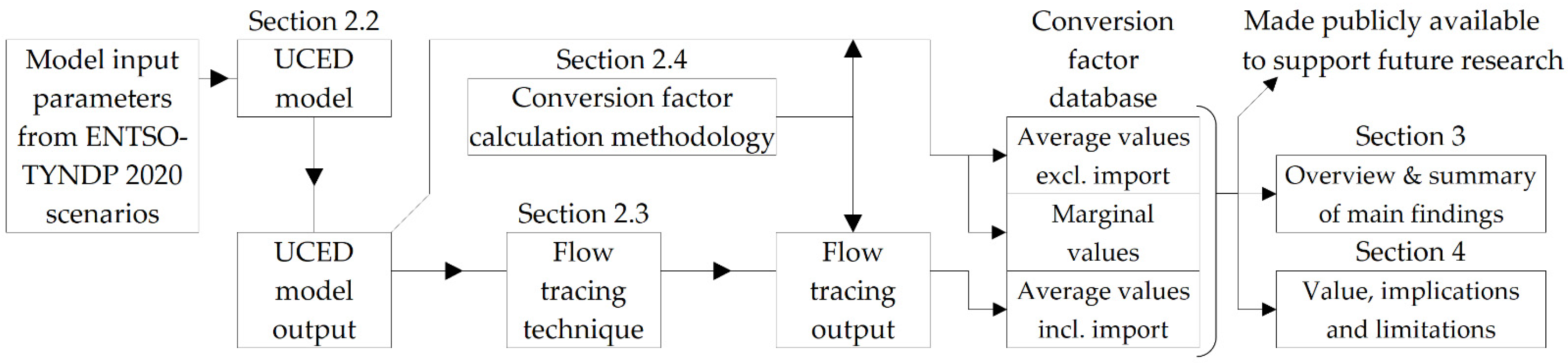
The methodology used to generate the conversion factor database consists of three main parts. The first and most important part is the development of a unit commitment economic dispatch (UCED) model to simulate the future European electricity system. In Section 2.2, the basic structure of the model and its features are explained, as well as the applied scenario framework. The goal of this detailed explanation is not only to allow for a correct interpretation of the results, but also to enable anyone who is interested to replicate the model—supporting future research in which there is a need to rigorously simulate the future European electricity system. The output of the UCED model lays the foundation for the calculation of the conversion factors, but in order to correctly take into account imports, another methodological step is required. This step is explained in Section 2.3, in which a flow tracing technique is innovatively applied to the output of the UCED model. Flow-tracing disaggregates the flows across the European network and determines—for each country and for every timestep—where the electricity it is importing was generated. Finally, Section 2.4 explains how the output of the UCED model and the flow-tracing technique is translated into conversion factor values. This includes an explanation of how both “average” and “marginal” conversion factors are calculated, as well as why (and how) two varieties of PEF values are calculated. Figure 1 presents a structural overview of the methodology, graphically illustrating the connection between the following Section 2.2, Section 2.3 and Section 2.4 as well as the final output of this exercise, namely the generated conversion factor database and the accompanying results and discussion sections.
2.2. UCED Model
A state-of-the-art UCED model is developed, to simulate the hourly dispatch of electricity generators in the future European electricity system. It includes 28 countries, namely 25 EU Member States (all but Malta and Cyprus), supplemented with Norway, Switzerland and the United Kingdom (UK). Model parameters are based on the scenarios established by the European Network of Transmission System Operators for Electricity (ENTSO-E), in its latest Ten Year Network Development Plan (TYNDP) 2020 report [54]. The report includes three scenarios. One covering the years 2025, 2030 and 2040, and two covering only the years 2030 and 2040. The former is called “National Trends” (NT), while the latter two are called “Distributed Energy” (DE) and “Global Ambition” (GA). These scenarios lay the foundation for a rigorous analysis of future conversion factors, covering a variety of potential directions in which the European system could evolve. While the NT scenario is compliant with the national energy and climate plans (NECPs), the DE and GA scenarios are compliant with the 1.5 °C target of the Paris Agreement and take into account the EU’s 2030 targets.
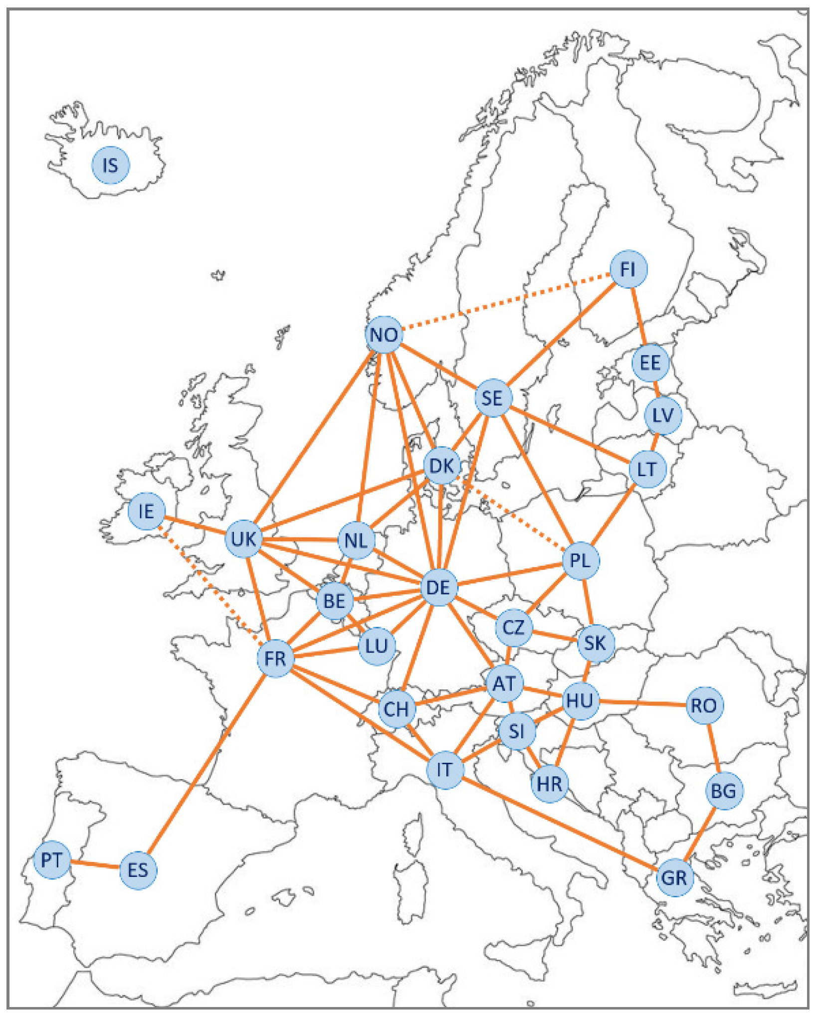
In addition to 28 country nodes, the UCED model contains 59 interconnecting lines, as shown in Figure 2. The transmission grids within countries are assumed to be “copper plates” and the interconnecting lines between any pair of two countries are aggregated (while, in practice, multiple separate lines may exist across the geographical border). These simplifications are necessary to keep the simulations computationally manageable, and because the ENTSO-E scenarios do not contain detailed representations of the national transmission grids (let alone distribution grids). Moreover, the goal of the UCED model is to estimate conversion factors at the national level—to support policy and technical analyses in need of them. The model’s focus therefore lies in accurately capturing national dispatching dynamics across 28 European countries. Both seasonally and at the hourly level, while taking into account imports and exports. The hourly temporal resolution is itself chosen because this is the resolution of the ENTSO-E electricity demand and renewable energy capacity factor profiles [54]. Sufficient input data at higher temporal resolutions is unfortunately unavailable, e.g., to simulate electricity markets clearing at 15-min intervals.
There are four motivations for choosing ENTSO-E’s scenarios to populate the model with appropriate parameters. First of all, the scenarios represent the combined expertise of 42 Transmission system operators, each contributing their own detailed knowledge about the electricity demand and generation capacities within their respective control areas. Secondly, the development of the TYNDP 2020 scenarios is supported by a substantial process of stakeholder consultation. Non-governmental organizations, various market parties and academics are all involved in reviewing and adapting the assumptions and hypotheses that go into the scenarios. Together with ENTSO-E’s considerable in-house expertise, this guarantees a best-possible effort to rigorously forecast the future European electricity system. Thirdly, the ENTSO-E scenarios contain the most expansive and detailed set of internally consistent assumptions and input variables:
- Installed capacities for an exceptionally disaggregated set of technologies (Table 1), including 15 types of gas plants and 12 types of coal plants.
- Detailed technical characteristics for every technology (including conversion efficiencies, start-up costs, start-up fuel consumption, variable operation and maintenance costs, minimum up times, minimum stable generation levels, maintenance requirements, forced outage rates and CO2 emissions factors)
- Hourly profiles for electricity demand and electricity generation by wind, solar and hydro technologies in every country (for 2025, 2030 and 2040)
- Net transfer capacities of the transmission lines interconnecting countries
- Fuel and CO2 prices (Table 2)
Finally, the ENTSO-E scenarios contain both forecasts based on policies as well as least-cost optimization. The NT scenario primarily consists of a “best estimate” of how the European system will evolve if all current and announced policies are implemented, while the DE and GA scenarios primarily rely on a “least-cost” investment optimization model to determine model parameters like installed capacities per generation technology and net transfer capacities. The value of the “best estimate” approach lies in its consideration for the observed and expected constraints on the speed and realization of the energy transition. Meanwhile, the “least cost” approach is more in line with established forecasting methods in the literature [56]. It presents a picture of a more ideal European system—both in terms of total costs and CO2 emissions—which could be realized with additional policies.

Table 1.
Overview of technologies included in the UCED model.
| Weather Dependent | Gas-Based | Coal-Based | Oil-Based | Other |
|---|---|---|---|---|
| Solar | Gas CCGT CCS | Hard coal new | Heavy oil old 1 | Nuclear |
| Solar Thermal | Gas CCGT new | Hard coal new Bio | Heavy oil old 1 Bio | Battery |
| Wind offshore | Gas CCGT new CCS | Hard coal old 1 | Heavy oil old 2 | DSR |
| Wind onshore | Gas CCGT old 1 | Hard coal old 1 Bio | Light oil | Other non-RES |
| Hydro PS (closed) | Gas CCGT old 2 | Hard coal old 2 | Oil shale new | Other RES |
| Hydro PS (open) | Gas CCGT old 2 Bio | Hard coal old 2 Bio | Oil shale new Bio | |
| Hydro Reservoir | Gas CCGT present 1 | Lignite new | Oil shale old | |
| Hydro RoR | Gas CCGT present 1 CCS | Lignite old 1 | ||
| Gas CCGT present 2 | Lignite old 1 Bio | |||
| Gas CCGT present 2 CCS | Lignite old 2 | |||
| Gas conventional old 1 | Lignite old 2 Bio | |||
| Gas conventional old 2 | ||||
| Gas conventional old 2 Bio | ||||
| Gas OCGT new | ||||
| Gas OCGT old |
Table 2.
Fuel and CO2 prices in the TYNDP 2020 scenarios.
| (€/GJ) | NT.2025 | NT.2030 | NT.2040 | DE.2030 | DE.2040 | GA.2030 | GA.2040 |
|---|---|---|---|---|---|---|---|
| Gas | 6.46 | 6.91 | 7.31 | 6.91 | 7.31 | 6.91 | 7.31 |
| Hard coal | 3.79 | 4.30 | 6.91 | 4.30 | 6.91 | 4.30 | 6.91 |
| Heavy oil | 13.26 | 14.63 | 17.21 | 14.63 | 17.21 | 14.63 | 17.21 |
| Light oil | 18.80 | 20.51 | 22.15 | 20.51 | 22.15 | 20.51 | 22.15 |
| Lignite | 1.10 | 1.10 | 1.10 | 1.10 | 1.10 | 1.10 | 1.10 |
| Nuclear | 0.47 | 0.47 | 0.47 | 0.47 | 0.47 | 0.47 | 0.47 |
| Oil shale | 2.30 | 2.30 | 2.30 | 2.30 | 2.30 | 2.30 | 2.30 |
| (€/tonne) | |||||||
| CO2 | 23 | 28 | 75 | 53 | 100 | 35 | 80 |
Note: Fuel prices do not differ across scenarios. Details on the methodology used by ENTSO-E to determine CO2 prices can be found in [57]. The modelling approach with respect to biofuels is explained in Appendix A.
For each of the included countries, the model contains a detailed representation of both the demand and supply sides. On the demand side, the hourly electricity profiles take into account expected trends in both the “traditional” electricity demand as well as the proliferation of heat pumps and electric vehicles. Given the variety of assumptions, the demand profiles vary across the three scenarios. Detailed information about how ENTSO-E produced the demand profiles can be found in the TYNDP 2020 methodology report [57]. On the supply side, evolutions in the installed capacities of all electricity generation technologies are considered—with a “best estimate” as well as a “least cost” approach (as explained above). In both cases, the projected phase-outs of coal and nuclear technologies (in certain countries) are considered as well. Moreover, it should be noted that all of the scenarios contain a sharp increase in renewable energy generation across Europe—although the precise amount differs from country to country. In [59], the current differences across European countries in terms of their renewable energy development are explored in detail, which can serve as a background to the developments that are forecasted in the scenarios simulated with the UCED model.
To simulate the dispatch of electricity generators as accurately as possible, the characteristics of all generation technologies are maximally taken into account. Weather-dependent technologies like wind, solar and run-of-river hydro are considered on a country-by-country basis. They are essentially modelled as “free” generators, and are therefore dispatched according to the hourly capacity factor profiles. These are based on historical weather data (as observed by satellites), but also considering technological improvements. For example, the profiles for offshore wind have higher capacity factors in 2030 than in 2025, reflecting the fact that offshore windmills become better over time at capturing the available wind.
Reservoir hydro also deserves careful attention, because it represents a significant share of total electricity production in several European countries (including Austria, Switzerland, Norway and Sweden). However, correctly simulating its role in the overall dispatch is challenging due to several aspects related to its complex nature. These include the size of the reservoirs and volumes of water they contain at the start of the simulation, as well as the natural inflows of water that occur throughout the year. Our model includes these elements, based on parameters found in the specialized hydro-database released by ENTSO-E [60].
The full simulation of the UCED model consists of three stages, whereby the output of each one feeds into the next. First, the model starts by considering the typical maintenance needs of every generator unit in the system, and optimally schedules maintenances across the year. Then the full year is simulated at once, applying only the linear optimization constraints and using a low temporal resolution of four time periods per day. Similar to the final phase, this simulation performs both unit commitment as well as economic dispatch. Typical examples of linear optimization constraints are a generator’s maximum generation capacity, starting costs and variable O&M costs. When MIP constraints like a minimum stable generation level or minimum up and down times are excluded, the simulation remains a linear optimization problem—which is easier to solve, but ignores dispatching dynamics that are important at the hourly level. The full-year simulation determines the optimal storage and utilization of energy in the hydro reservoirs across the year. Finally, the hourly simulation is executed in full detail. This consists of a mixed integer program (MIP), in which the optimization objective is to minimize the total cost of electricity generation. Technical constraints of the generators and interconnection lines need to be respected and a high cost is associated with failing to meet the hourly electricity demand in any particular country. Further details on our UCED model are provided in Appendix A, which includes both a more comprehensive explanation of some of the modelling aspects already explained, as well as additional information about the modelling of non-renewable technologies and the applied simulation tool—PLEXOS (developed by Energy Exemplar, https://energyexemplar.com accessed on 6 March 2021).
2.3. Flow Tracing
To estimate future national conversion factors taking into account imports from other countries, the UCED model on its own is not sufficient. The output of the UCED model is limited to the generation by each technology in every country, as well as the flows on the interconnecting lines—for every hour. In itself, this does not reveal where the electricity consumed in each country was produced. For example, Portugal may be importing from Spain, but this electricity may have been (partially) produced in France. To estimate a conversion factor of electricity consumed in Portugal (e.g., its CO2 intensity), information is required about how much of the imported energy was generated in Spain, France and elsewhere in Europe. It is a feature of any traditional UCED model that it cannot produce such information on its own.
A technique called flow tracing is required to find out where the electricity imported and consumed in any given country was effectively produced. This allows conversion factors to be distinguished from two perspectives. From a production perspective, conversion factors only consider the electricity produced within a given country. From a consumption perspective, conversion factors consider the electricity imported from other countries as well. For example, while the electricity produced in Belgium may have a CO2 intensity of 100 kg/MWh, electricity consumed in Belgium may have a CO2 intensity of 200 kg/MWh, if 50% of electricity is imported from a country with a more carbon-intensive electricity production mix (300 kg/MWh). To take into account cumulative grid-losses of 10% across transmission and distribution—as proposed by [24]—consumption perspective values are multiplied by a factor of 1.1. Figure 3d illustrates how production- and consumption-perspective values can differ from each other on an hourly basis.
Several recent studies have already adopted the flow tracing technique and explained it in detail [61,62,63,64,65]. As described in these studies, flow tracing essentially consists of creating and solving a system of linear equations, in which there are a number of known and unknown variables. The known variables are the electricity generation and demand in every country, as well as the flows on every interconnecting line (i.e., the output parameters of the UCED model). The unknown variables are the shares of each country’s electricity generation in every total line flow. Solving this system of equations could for example reveal that a total of 1.000 MWh being imported by Portugal from Spain, consists of 600 MWh produced in Spain, 300 MWh produced in France and 100 MWh produced in Belgium. Figure 3c visualizes this type of disaggregation.
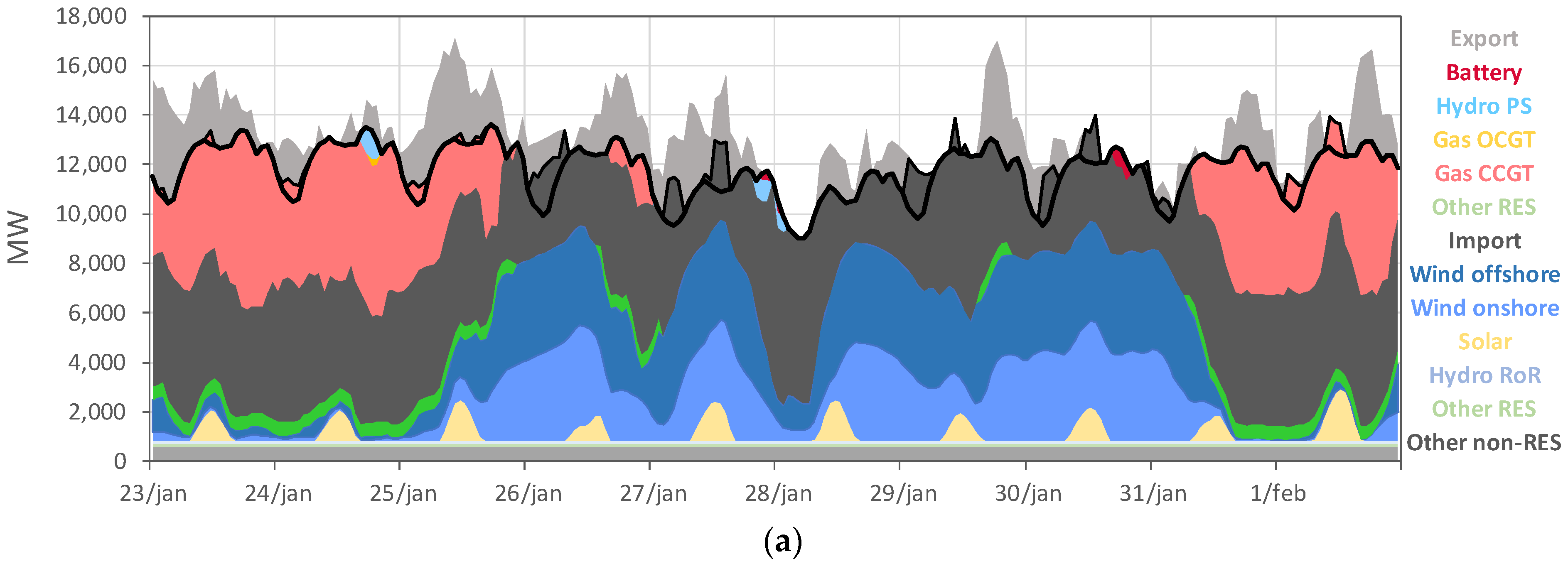
In its entirety, Figure 3 provides an overview of the functioning of the UCED model and the application of the flow tracing technique for an illustrative period of ten days. The electricity generation taking place in Figure 3a is translated directly into the production perspective conversion factors shown in Figure 3d. Meanwhile, net imports shown in Figure 3b are disaggregated using flow tracing (Figure 3c), to derive the consumption-perspective conversion factors shown in Figure 3d—which also shows how the estimated hourly PEFs can differ, depending on the applied calculation methodology (Section 2.4).
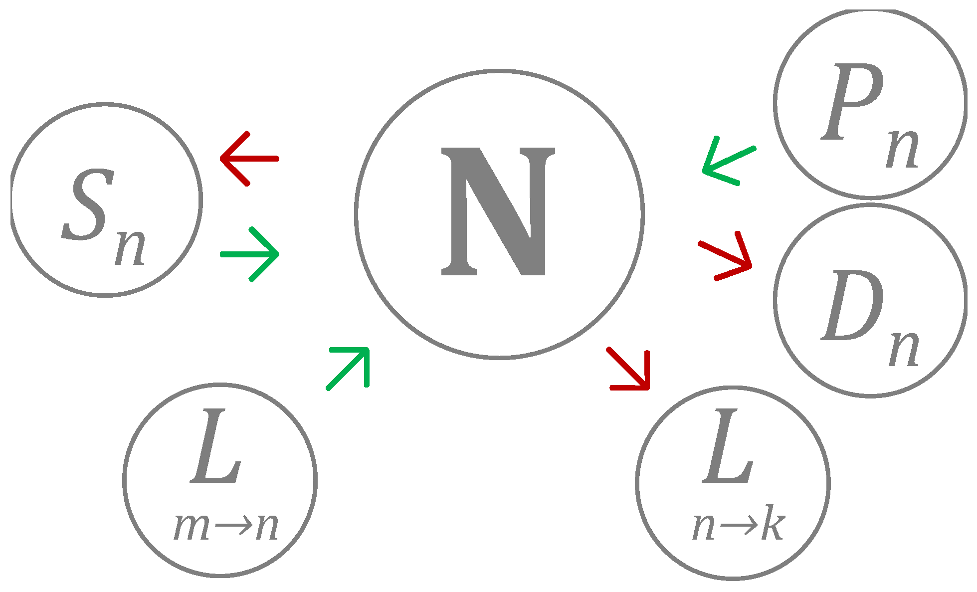
Flow tracing requires that two assumptions are made. The first is a simplified interpretation of Kirchhoff’s current law, namely that the sums of all incoming and outgoing flows at any given (country) node must be equal to each other (Figure 4). The second assumption is the principle of proportional sharing between incoming and outgoing flows at any node. This means that all incoming flows are evenly “mixed” at the node, and spread across the outgoing flows.
Figure 4 depicts a generic country node N, accompanied by a number of incoming and outgoing flows. At every such country node, the sums of incoming (green) and outgoing (red) flows must always be equal. Incoming flows originate first and foremost from the electricity production by country N’s regular generators (Pn) and storage generators (Sn). Batteries and pumped hydro technologies are both examples of storage generators. Other incoming flows come from the interconnecting lines between N and other countries. For example, there may be an incoming flow on the interconnecting line with country M (Lm->n). All incoming flows are evenly mixed and spread proportionally across the different outgoing flows. These are the electricity demand in country N (Dn), the electricity demand from large-scale storage generators in country N (Sn) and the outgoing flows on interconnecting lines—for example towards country K (Ln->k).
Previous studies have only applied the flow tracing technique to historical electricity generation data, to determine the differences between production and consumption perspective CO2 intensities across Europe for the year 2017, and across the United States for the year 2016 [63,65]. However, flow tracing can also be applied to the output of UCED simulations of future electricity system scenarios. In fact, the increasing interconnectivity and cross-border trade within the future European electricity system makes it even more relevant to apply flow tracing and consider conversion factors from a consumption perspective. Moreover, the fact that previous flow-tracing studies have only focused on CO2 intensities forms another limitation [63,65], given the fact that it is equally relevant to apply the technique to the estimation of primary energy factors. Similar to the fact that it is worth knowing the consumption perspective CO2 intensity associated with charging an electric vehicle, it is worth knowing the consumption perspective PEF when the primary energy use associated with a building is estimated. To the author’s best knowledge, the present study is not only the first one to apply flow-tracing to future scenarios for the European electricity system, but also the first one to use the technique to calculate both CO2 intensities and PEFs from a consumption perspective.
2.4. Calculation of Conversion Factors
2.4.1. Average Values
Average conversion factors relate to the entire electricity mix. They are calculated according to the following formula, using PEF as an example (the method for CO2 intensities is analogous):
The PEF for electricity produced in country i, timestep t, is calculated as a weighted average, taking into account the electricity production (P) by each generator j that is located in the country, its respective technology-related PEF (PEF′), and the total electricity production in the country (TP). In the case of a consumption perspective, net import is considered as an additional technology—the conversion factor of which is found through flow tracing (Section 2.3)—and TP is replaced with total consumption.
Conversion factors can be calculated for any timestep, including hours, seasons or the entire simulated year. They can also be calculated for the UCED model’s 28-country region in its entirety. In each case, the share of every generation technology in the total amount of electricity—Equation (1)’s denominator—is accurately taken into account. This means that a yearly conversion factor is not simply the average of hourly values across the year, and a European-level conversion factor is not simply the average of national values. Extrapolations across both time and space are appropriately weighed.
Table 3 presents an overview of the assumptions used for each technology. For thermal generation technologies, the PEF is based on the conversion efficiency. For example, the PEF for nuclear is 3, based on the assumed conversion efficiency of 33% (1/0.33 = 3), meaning that 3 units of primary energy are consumed for every unit of electricity produced by nuclear generation units in the UCED model.
For wind, solar and hydro technologies, a PEF value of either 0 or 1 can be chosen. Both options are methodologically valid, although a value of 1 is chosen most often [66]. The associated debate revolves around the question of whether or not a unit of primary energy is “consumed” (in the same sense of a thermal generator consuming its fuel) when a wind, solar or hydro generator produces a kWh of electricity. Assuming a value of 1 is called the “direct equivalent” or “physical energy content” method, which is used by Eurostat and the IEA [66]. Assuming a value 0 is called the “zero equivalency method”, which is sometimes used in the building-related energy literature [25,27,30]. Due to the large impact of this methodological choice on the overall PEF of electricity—especially in future scenarios with a higher penetration of renewables—results are generated using both options (Section 3.6).
For the technologies left out of Table 3, the following assumptions are made—in line with the TYNDP 2020 scenarios. Bio varieties are assumed to have a PEF equal to their traditional counterparts, and a CO2 intensity of 0. Varieties using carbon capture and storage (CCS) have a slightly worse conversion efficiency (i.e., a slightly higher PEF) and an approximately 90% lower CO2 intensity. The technologies “Other RES” and “Other non-RES” are assumed to have a PEF of 2.2. In terms of CO2 intensity, “Other RES” is assumed to have a value of 0, while the value of “Other non-RES” varies between 100 and 600 kg/MWh—depending on the scenario.
2.4.2. Marginal Values
Marginal conversion factors relate to the marginal electricity generation technology. They are simply equal to the PEF or CO2 intensity of whichever technology is marginal during a particular hour. Due to the fact that the marginal technology can change from hour to hour, it does not make conceptual sense to estimate a marginal technology for longer time periods like seasons or an entire year. Neither does it make sense to distinguish between a production and consumption perspective. The question answered by a marginal conversion factor is “Which technology will adjust its electricity generation, given a change in demand?”, which—by definition—requires a consideration of imports. The marginal generation technology can always be located in a different country.
To derive the marginal technology during every hour of the UCED simulations, the wholesale price in every country can be used as a proxy. Whenever a country is importing electricity, the marginal and price-setting technology is located in a different country. This is the nature of the locational marginal pricing algorithm, which is used in the UCED model to reflect real-life wholesale pricing to a satisfactory degree. Every technology in the UCED model has its own unique marginal generation cost, due to the combination of conversion efficiencies, variable operation and maintenance (O&M), fuel and CO2 costs.
The UCED model’s precise disaggregation of technologies is valuable in this context, because it enables a wider variety of marginal conversion factors to be identified. This is more in line with reality and allows for a more precise optimization of controllable electricity demand by individual market participants. If, for example, the applied UCED model would aggregate all “gas” technologies, then the derived marginal conversion factors would be extremely unprecise. As shown in Table 3, a variety of CO2 intensities and PEFs are associated with gas-based generation technologies.
3. Results
3.1. Overview
Results are generated for all seven scenario-years contained in the TYNDP 2020 framework [57]. The term “scenario-year” is used to refer to the simulation of a particular combination of a scenario (e.g., “National Trends”) and a year (e.g., 2025). The full list of scenario-years is NT.2025, NT.2030, NT.2040, DE.2030, DE.2040, GA.2030, and GA.2040. In each scenario-year simulation, nine varieties of conversion factors are calculated for each of the 28 countries. First of all, there are two varieties of PEFs (cf. Section 2.4.1). Together with the CO2 intensities, this leads to a sub-total of three conversion factor varieties. Secondly, average and marginal varieties of each three exist, leading to a sub-total of six. Finally, the average varieties can be further distinguished into values from a production and a consumption perspective (cf. Section 2.4), leading to a total of nine conversion factor varieties. Given the large amount of scenario-years, countries and conversion factor varieties, the total output contains approximately 15 million hourly conversion factor values.
The following sections provide a summarizing overview of these values—focusing on a number of figures that highlight important findings. An exhaustive discussion and explanation for every result is infeasible within the constraints of the present paper, which is why several of the figures in this section are limited to an illustrative subset of the 28 countries contained in the UCED model. However, the complete output database is made publicly available so it can be examined in full detail by anyone interested in specific conversion factors (e.g., for a particular country in a particular scenario-year). The complete conversion factor database can be found on the following URL: http://bit.ly/3uCLx0x (accessed on 6 March 2021).
Section 3.2, Section 3.3, Section 3.4, Section 3.5 and Section 3.6 discuss average conversion factors (which consider the entire electricity mix). Unless explicitly stated otherwise, all the discussed values of conversion factors represent a consumption perspective (whereby the influence of imported electricity is taken into account). Moreover, all PEF values discussed in Section 3.2, Section 3.3, Section 3.4 and Section 3.5 are estimated assuming a value of 1 for hydro, wind and solar. PEF results where the less conventional value of 0 is assumed, are discussed separately in Section 3.6. Marginal conversion factors are also discussed separately, in Section 3.7.
3.2. General Future Evolution of Conversion Factors across Europe
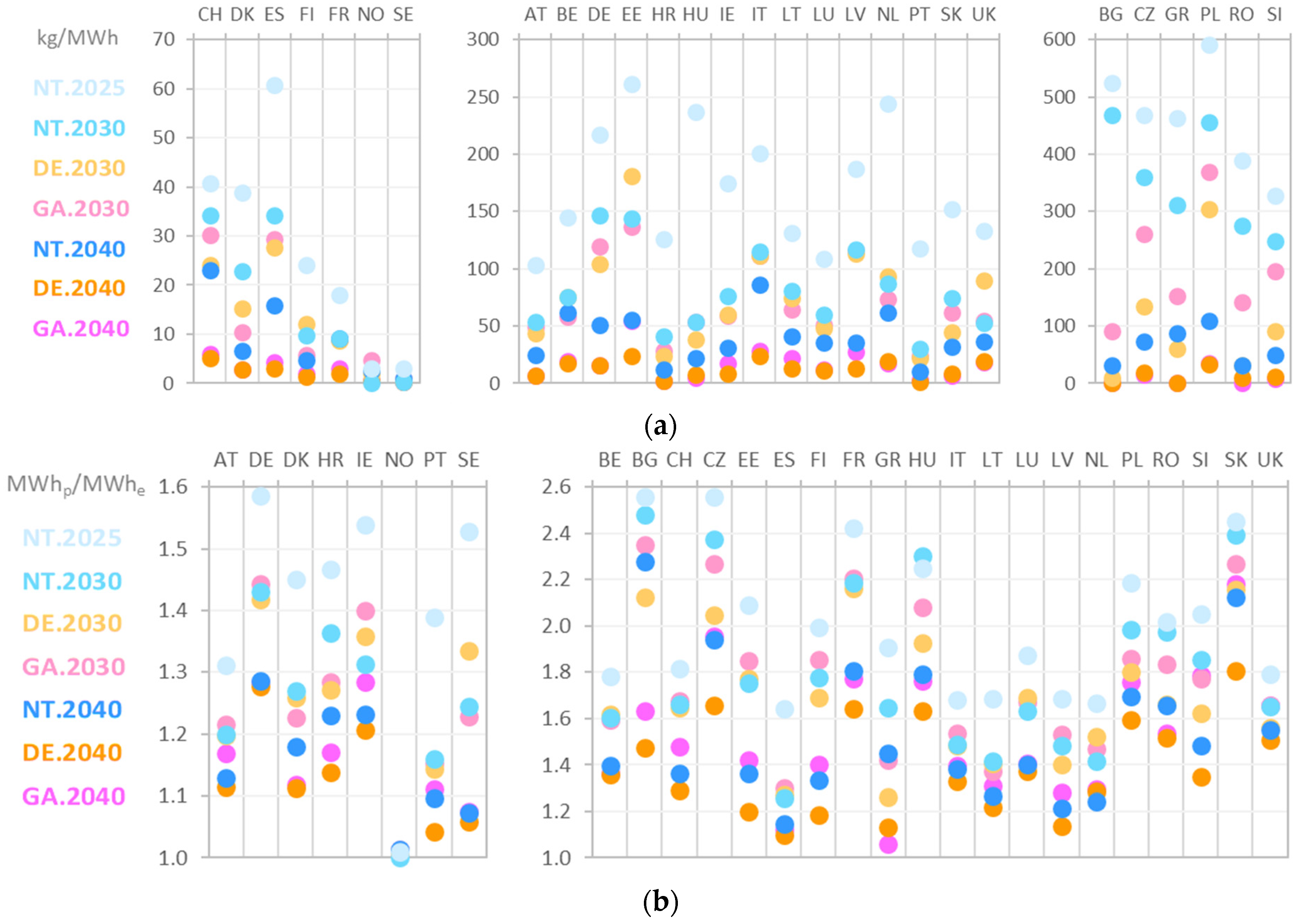
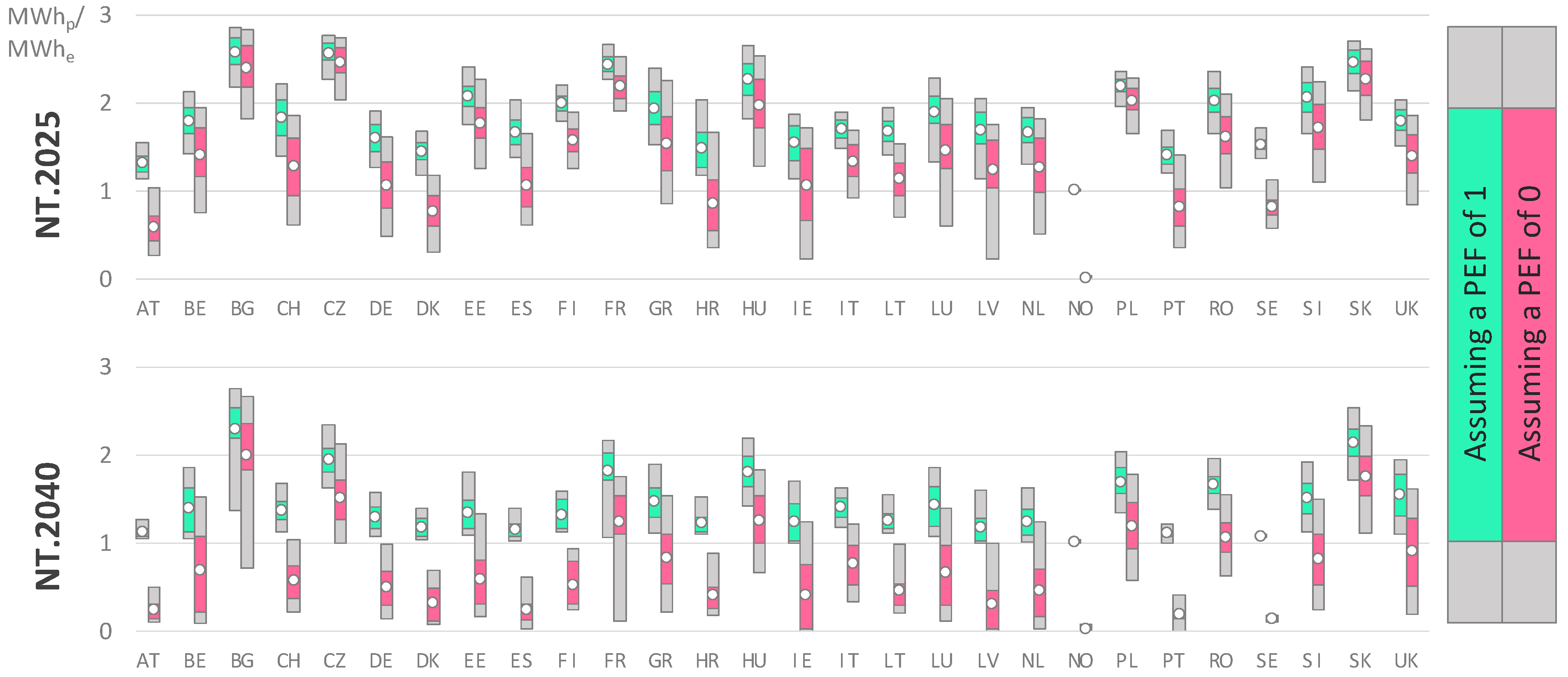
Yearly conversion factors can be expected to decrease significantly between 2025 and 2040—mainly driven by the increasing electricity generation by wind and solar technologies—although we find a considerable heterogeneity across individual countries (Figure 5a,b). Countries are grouped according to similar values, so differences across scenario-years can be clearly distinguished. In the year 2025, a number of countries have CO2 intensities that are already below 50 kg/MWh while others range between 300 and 600 kg/MWh. All CO2 intensities decrease dramatically by the year 2040, although in some cases (Czechia, Greece and Poland in NT.2040) values are still higher than those of others in 2025 (Norway and Sweden). A similar dynamic is observed in the case of PEFs.
For the years 2030 and 2040, the three scenarios provide insight into the uncertainty of the conversion factor estimates. For many cases, uncertainty is limited—for example in the case of PEFs for Germany, Belgium, Spain, Italy, and the UK. In other cases, uncertainty is rather high—for example, the CO2 intensity for Czechia. For the year 2030, it is as high as 360 kg/MWh in the National Trends scenario, but as low as 134 kg/MWh in the Distributed Energy scenario. This can be explained by the difference in installed capacities for solar PV (4900 MW in NT.2025 versus 10,500 MW in DE.2030).
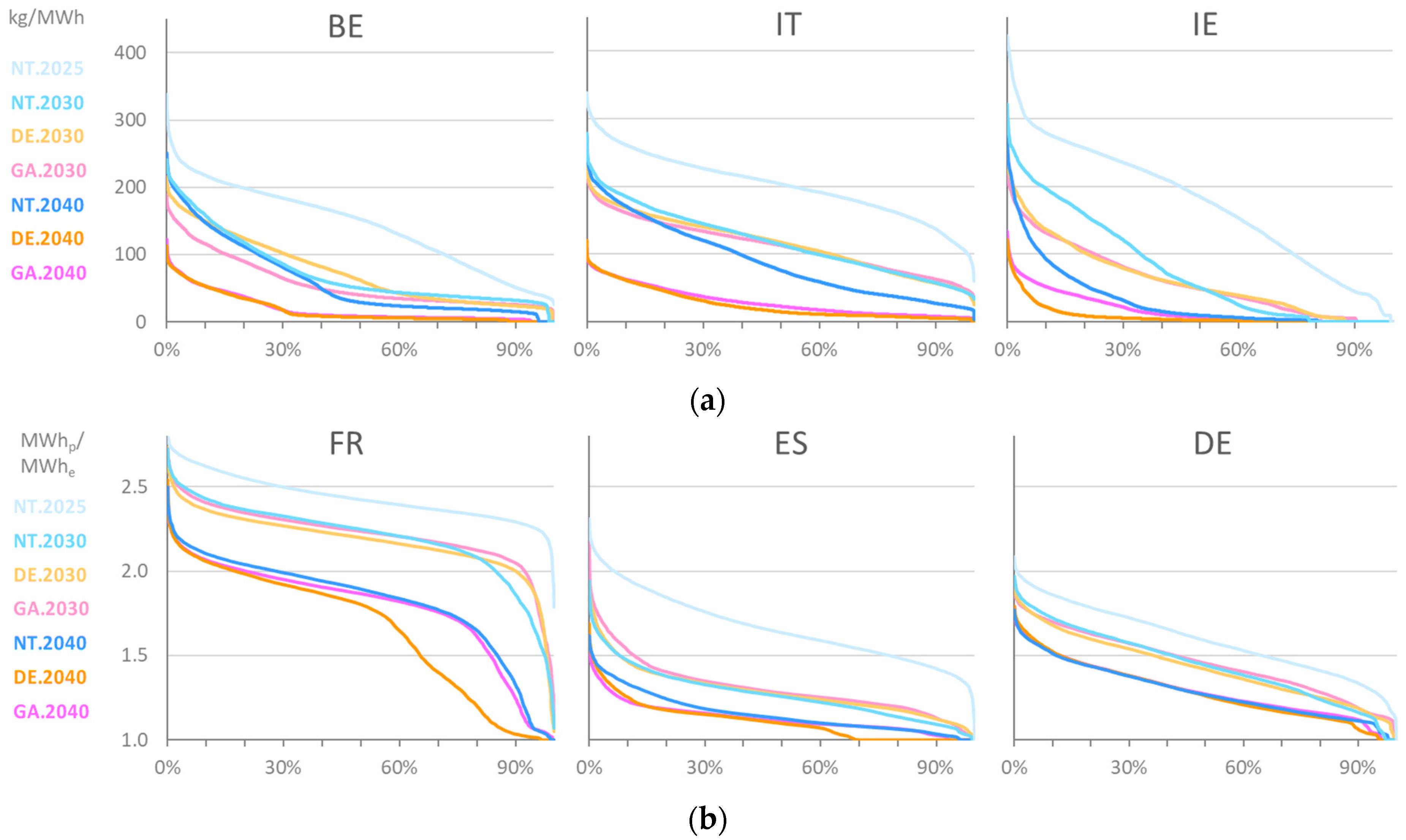
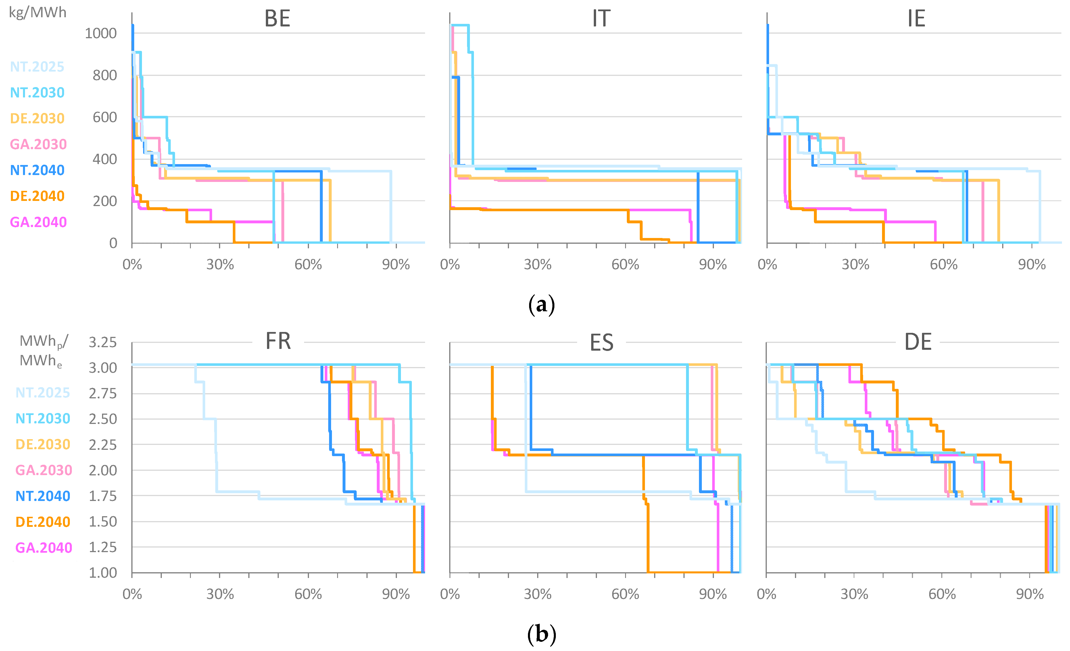
In addition to the general trend in terms of yearly conversion factors, changes are also found in terms of the distribution of values within each year (Figure 6a,b). As indicated by the sample of countries, this is another way in which conversion factors vary significantly across Europe. All hourly values are plotted as duration curves, meaning that they are ordered from large to small. This shows that the CO2 intensity in Belgium is close to 0 kg/MWh for approximately 70% of the time in DE.2040 and GA.2040. Across scenarios, the duration curves for a particular year mostly overlap, with a few exceptions. Namely, in the case of CO2 intensities for Ireland, and PEFs for France. Here as well, differences can be attributed to the installed capacities assumed in each scenario. For example, the cumulative capacity of wind and solar technologies in France is 127 GW in NT.2040, 99 GW in GA.2040, and 174 GW in DE.2040. An alternative way of visualizing the distribution of values within each year—which is useful to derive further insights into the results—is presented in Appendix B.
3.3. Seasonal Variability of Conversion Factors
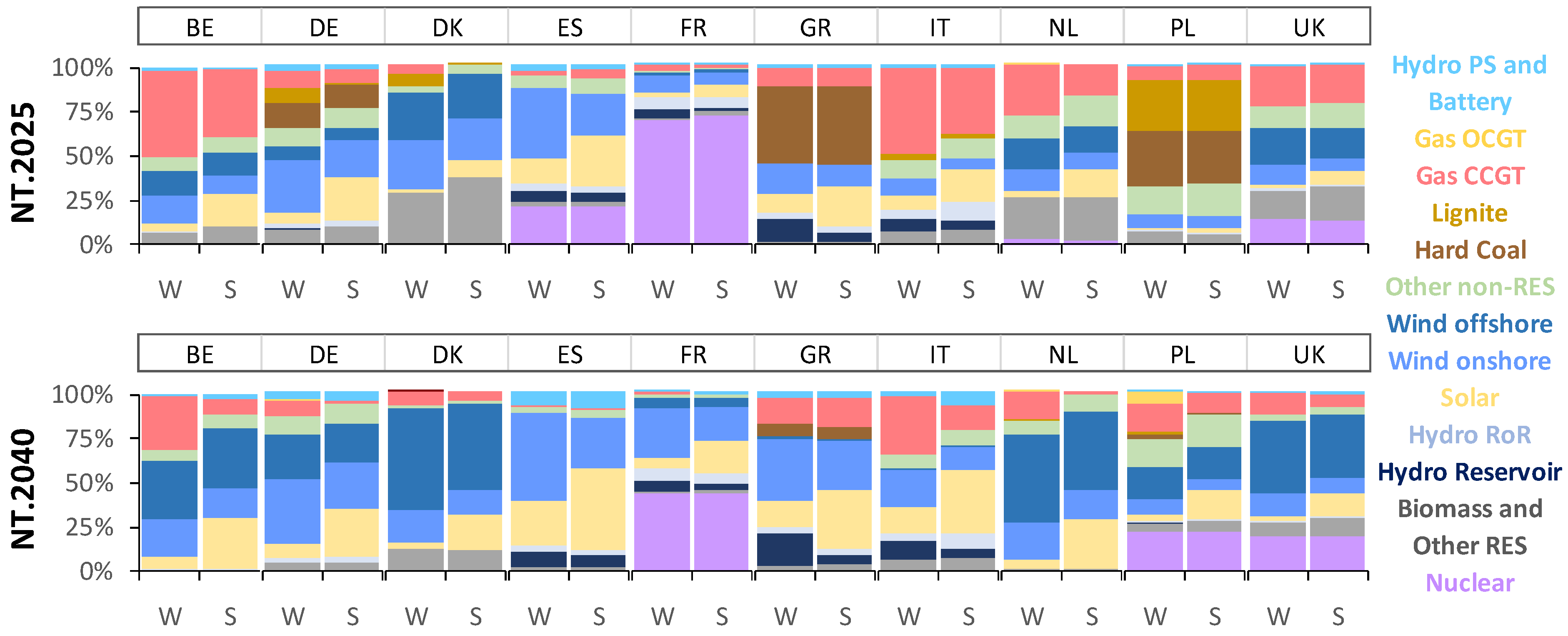
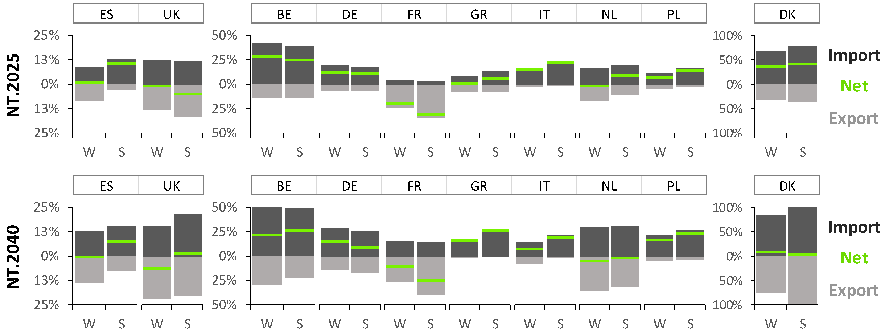
Conversion factors can fluctuate on a seasonal level, due to changes in the electricity generation mix throughout the year. Across countries, electricity demand may peak in either winter or summer, depending (among other things) on peaks in the heating and cooling needs of national buildings stocks. On the supply side, solar generation peaks in summer while wind generation typically peaks in winter (Figure 7). The combined effect of seasonal dynamics on the demand and supply sides differs from country to country. Moreover, countries can strengthen or counteract these effects through imports and exports—which show a degree of seasonality themselves (Figure 8).
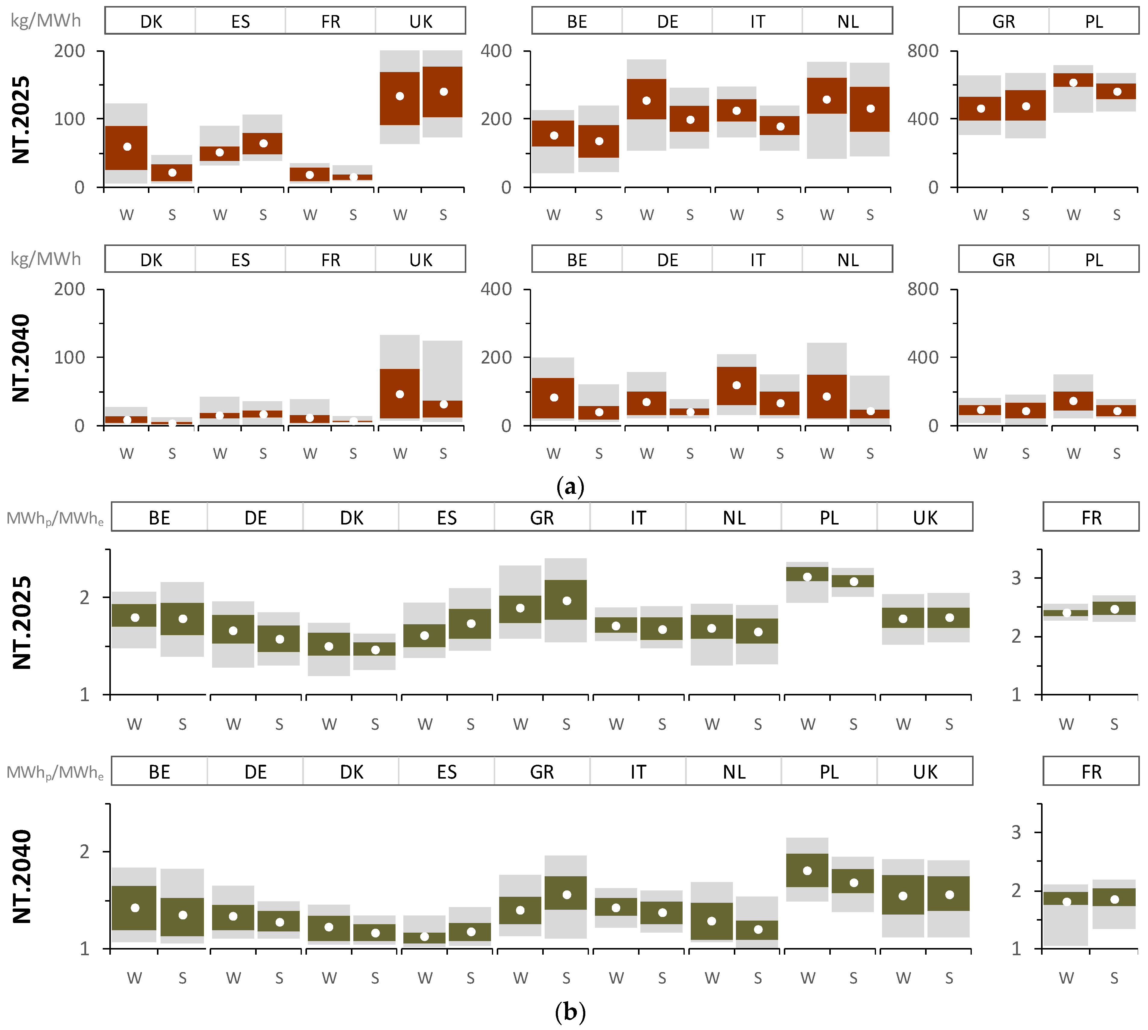
In terms of CO2 intensities, strong seasonal dynamics are observed in several countries (Figure 9a). For example, Danish hourly values show more variability and are higher on average in the winter than in the summer (NT.2025)—which is explained by differences in the generation by coal and gas technologies. In Spain on the other hand, the CO2 intensity is higher—on average—in the summer (NT.2025). Cumulatively, Spanish renewables cover a smaller share of demand in the summer, while the share covered by gas-based generators is higher. Both Belgium and The Netherlands only show a limited seasonality in NT.2025, but a large one in NT.2040. For Greece and Poland, the overall drop in CO2 intensities—from NT.2025 to NT.2040—is a lot more pronounced than the changes to their seasonality.
Seasonal dynamics can also be observed in the case of PEFs (Figure 9b). Here as well, changes in the electricity mix result in values that are higher in the summer (as in Greece) or the winter (as in Poland). The degree of variability within each season is different across countries here as well. While Belgian PEF values are more variable in the summer (NT.2025), German and Danish values are more variable in the winter. Meanwhile, French values decrease significantly for both seasons between NT.2025 and NT.2040. They also become a lot more variable, especially in the winter.
3.4. Hourly Variability of Conversion Factors
Figure 3a–d illustrates the translation from the output of the UCED model and the flow tracing technique to hourly CO2 intensities and PEFs for a sample period of ten days (Belgium in the scenario-year NT.2030). As shown in the bottom part of the Figure 3d, hourly conversion factors can fluctuate heavily on an hourly basis—although they can also remain relatively stable for a period of several days. Due to the combination of three phenomena, hourly conversion factors typically do not exhibit repetitive patterns. Namely, the variability of load, imports and renewable energy generation (especially from wind, which does not have a repetitive daily cycle like solar).
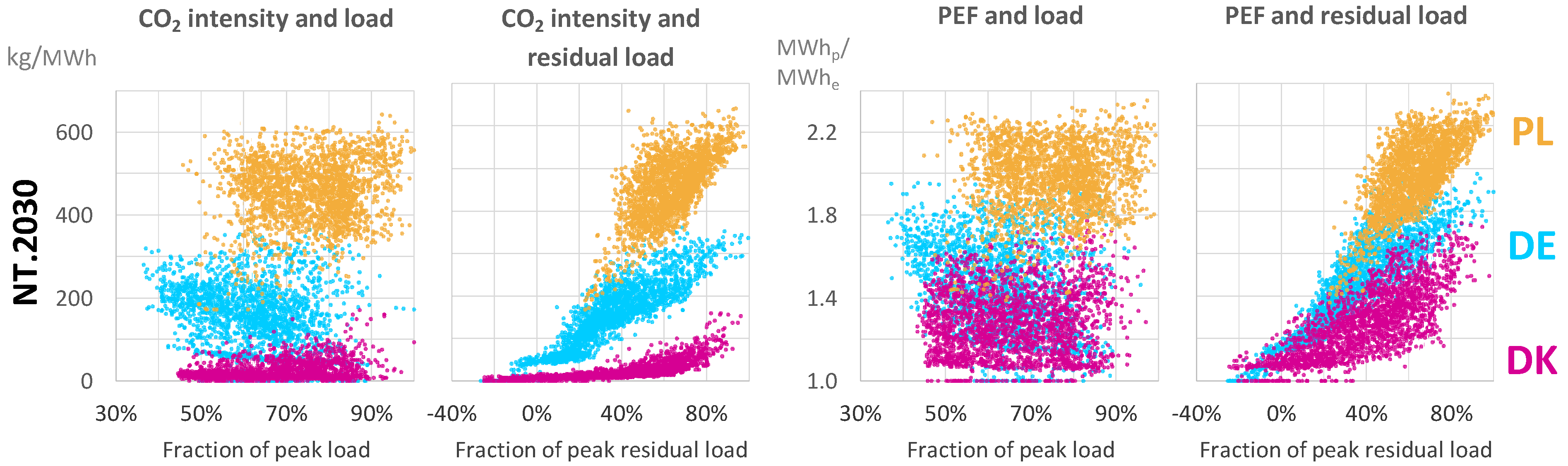
In theory, an isolated country that does not make use of renewable electricity technologies—instead using only a combination of traditional controllable technologies (e.g., nuclear, coal, and gas)—can be expected to have conversion factors correlating heavily with the hourly load. However, this type of correlation is almost completely missing in the interconnected future European electricity system (Figure 10). Within such a system, conversion factors only correlate clearly with residual load. As shown for Poland, Germany, and Denmark, hours in which wind and solar technologies are covering a large part of the national load (i.e., hours with a low residual load) correlate with low CO2 intensities and PEFs—and vice versa.
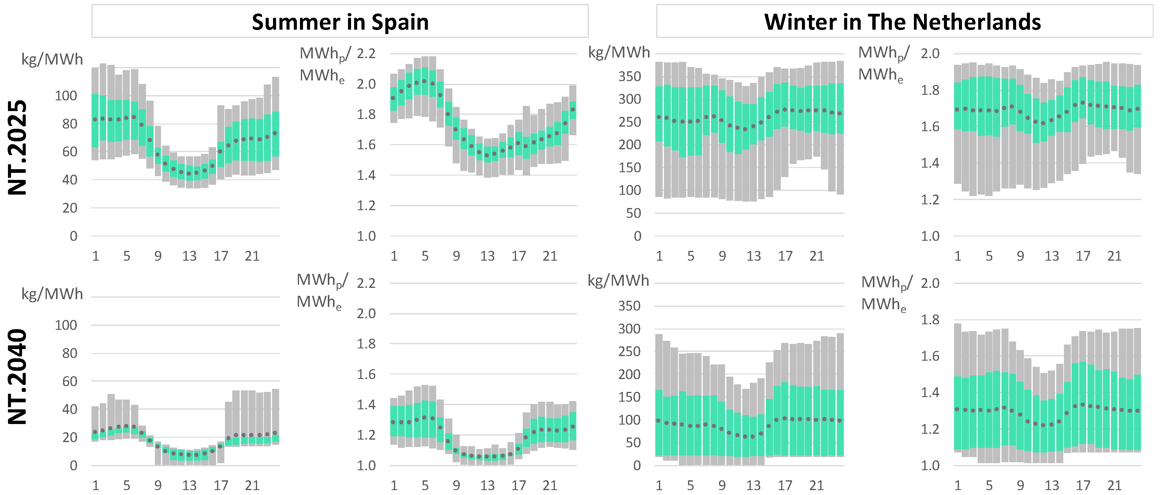
In terms of repetitive daily patterns in hourly conversion factors, the primary element to consider is the generation of solar technologies. Countries with a significant share of solar PV experience distinctive patterns—especially in the summer (Figure 11). For example, Spanish conversion factors are consistently lower during midday hours in the summer. On the other hand, countries in which the dominant renewable energy source is wind energy—which typically peaks in the winter—do not experience daily patterns to the same degree. For example, Dutch conversion factors are highly variable in almost every hour of the day (as shown in the winter period)—in NT.2025 as well as NT.2040. The hourly variability of wind generation does not have a distinctive daily cycle, unlike solar.
3.5. Impact on Conversion Factors of Taking into Account Imports
As discussed in Section 2.3, conversion factors cannot only be calculated from a production perspective—in which only the electricity production within a given country is considered—but also from a consumption perspective—in which imported electricity (and how it was generated) is also taken into account. While the former can be calculated purely from the output of the UCED model itself, the latter is calculated using the explained flow tracing technique.
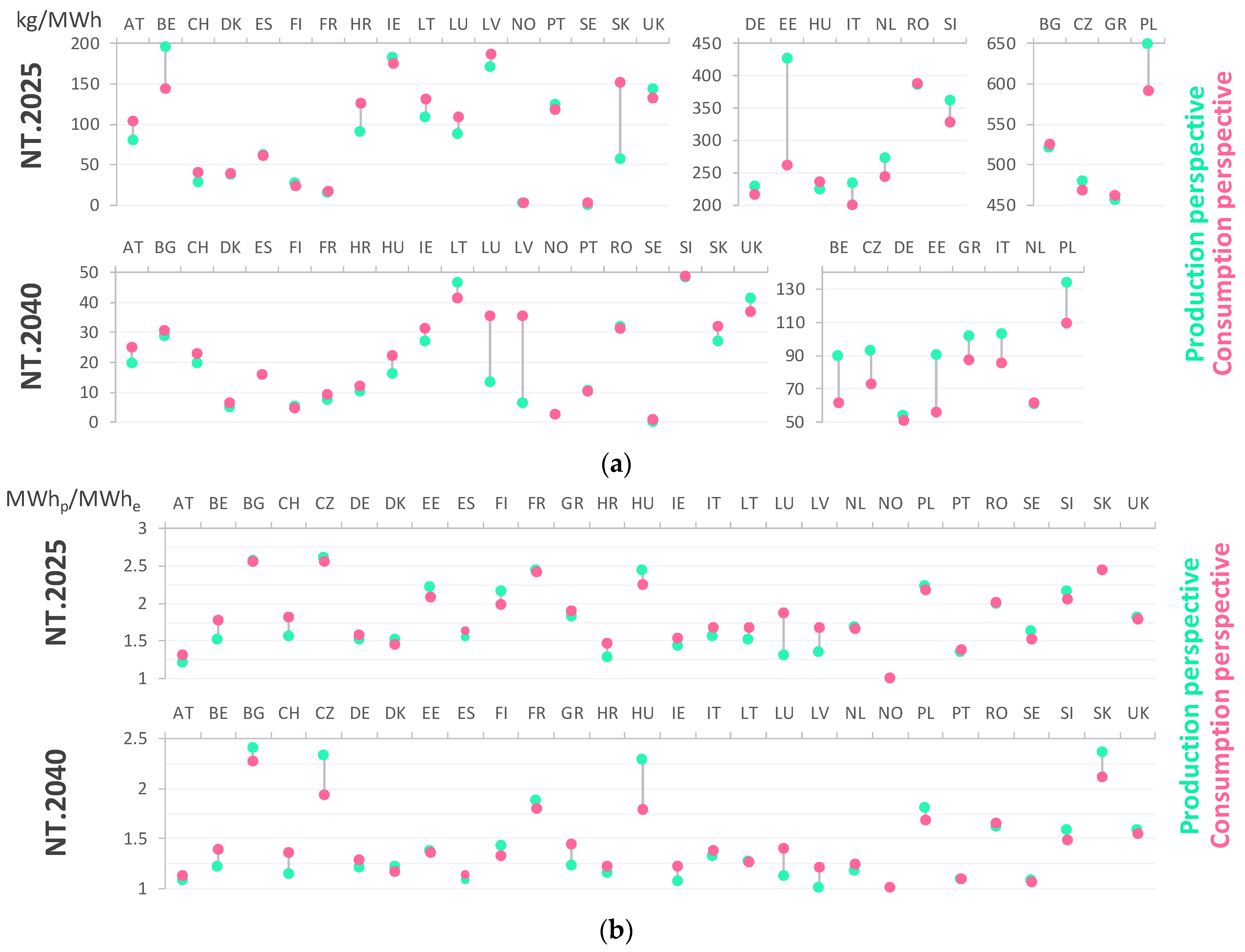
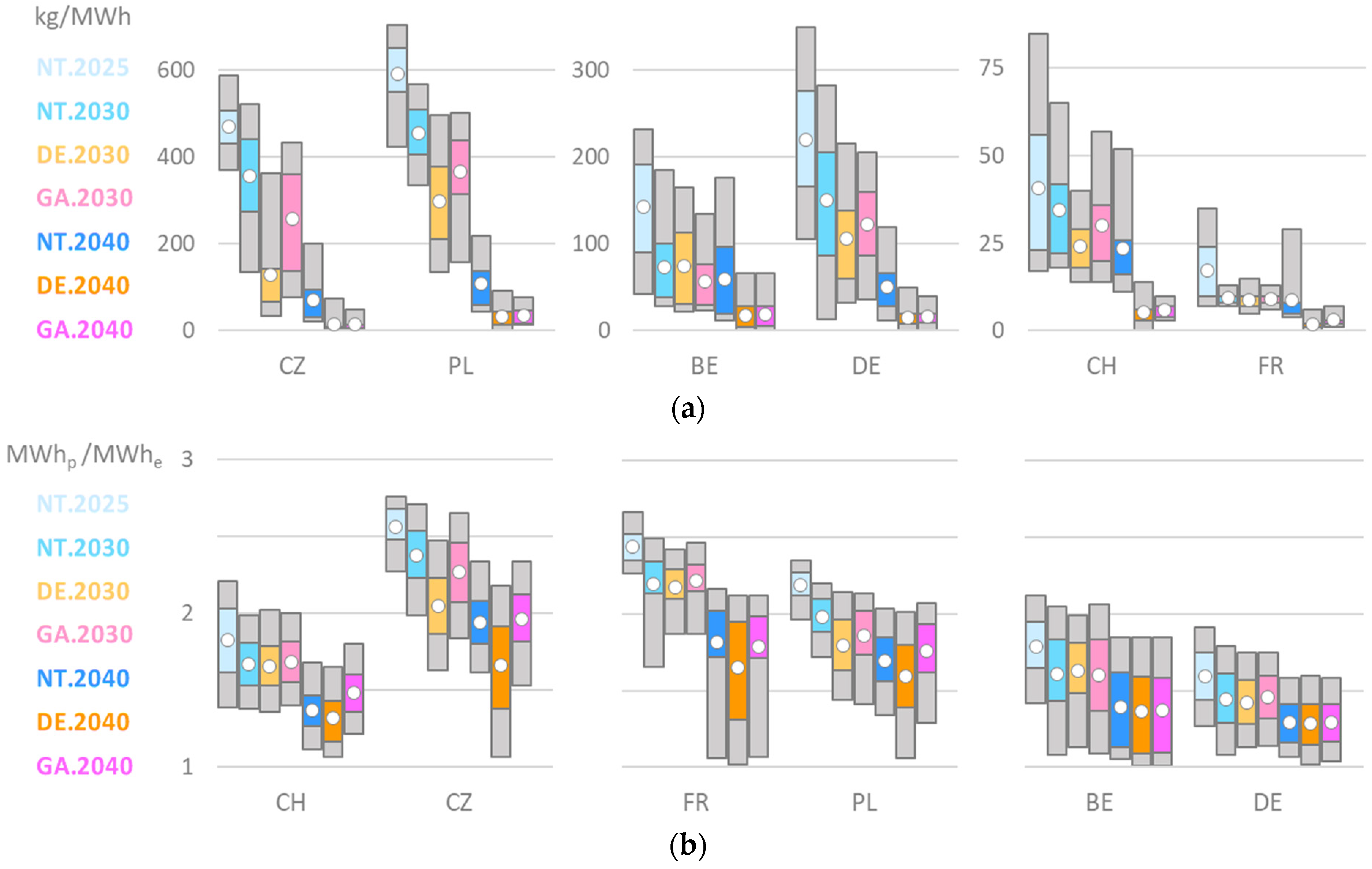
Taking into account imports can have a significant effect on yearly conversion factors, although the degree to which differs from country to country and across different scenario-years (Figure 12a,b). For most countries, both CO2 intensities and PEFs tend to increase when imports are taken into account, with a few notable exceptions. For example, the CO2 intensity in Belgium (NT.2025) is 195 kg/MWh from a production perspective, but only 145 from a consumption perspective (−26%)—largely due to imported electricity from France.
Whether or not it is important for a country to take imports into account, sometimes depends on the considered conversion factor. For example, the Hungarian CO2 intensity in NT.2040 is increased from 16 to 22 kg/MWh, which can presumably be ignored because the CO2 impact at such a low intensity is negligible. But the Hungarian PEF is decreased from 2.3 to 1.8 MWhp/MWhe, which can have a considerable impact on the primary energy estimation for a building, especially if it uses an electricity consuming heat pump. As another example, the PEF in Estonia is only decreased from 2.2 to 2.1 MWhp/MWhe by taking into account imports (NT.2025), but the CO2 intensity is decreased from 426 to 262 kg/MWh. Such a change has significant consequences when calculating the CO2 emissions associated with an individual electric load, like the charging of an electric vehicle.
Differences between production and consumption perspective conversion factors mainly depend on two things. Namely, whether a country imports a lot of its consumed electricity, and whether there are stark differences (in terms of conversion factors) with the countries it imports from. Countries differ significantly in terms of how much they import. For example, Belgium is typically a net importer, while France is a net exporter (as indicated by Figure 8). Total cross-country exchanges of CO2 and primary energy are discussed in Appendix C.
3.6. Impact of the Assumed Value for Hydro, Wind and Solar on overall PEFs
Assuming a value of 0 instead of 1 MWhp/MWhe in the calculation of the overall PEF of electricity is found to have a significant impact (Figure 13). On an hourly basis, the average PEF is sharply reduced, and its variability is increased. This is especially the case in the scenario-years with a higher penetration of renewables. For example, in The UK the average drops from 1.6 to 0.9 MWhp/MWhe. Meanwhile, the range between the 5th and 95th percentile values changes from 1.1P5–2.0P95 to 0.2P5–1.6P95 MWhp/MWhe (NT.2040). The higher variability is also illustrated for Belgium in Figure 3d (NT.2030). As the generation by wind technologies fluctuates throughout the sampled ten-day period, the hourly conversion factor profiles fluctuate more intensely as well.
3.7. Marginal Conversion Factors
Marginal conversion factors are significantly higher than average ones (Figure 14a,b). The number of unique hourly values is also limited by the number of potentially marginal technologies, resulting in more discrete duration curves. In several countries, national dispatching and importing dynamics need to be considered carefully to explain the marginal conversion factor profiles.
In Belgium, the marginal CO2 intensity in NT.2030 is 0 kg/MWh for approximately 50% of the time, which results from a combination of hours in which wind, solar, biomass, or nuclear technologies are marginal. In the case of nuclear, the Belgian marginal CO2 intensity is often set by importing from France. Meanwhile, France is found to have significantly fewer hours in which nuclear is the marginal technology in NT.2025 (compared to the other scenario-years). This can be explained by the fact that NT.2025 contains less wind and solar generation. In the other scenario-years, these renewable technologies more frequently push fossil technologies out of merit, resulting in French nuclear generators becoming marginal most of the time. Finally, marginal PEFs in Germany tends to increase over time, especially in the Distributed Energy and Global Ambition scenarios. This implies that the dynamics in these scenarios result in nuclear and fossil technologies with a high PEF value being marginal more often in Germany.
4. Discussion
4.1. Overall Value of the Results
The variability of conversion factors across time and space confirms the added value of the applied spatiotemporal scope. The estimated CO2 intensities and PEFs can be used in a variety of future research. For example, calculations about the CO2 emissions associated with charging an EV or about the primary energy use of an individual building can choose from a multitude of available conversion factors, analyzing the differences they make in the results. Additionally, conversion factors for different timeframes or countries can be used, or a choice can be made between average and marginal values, or between production and consumption perspective values.
Moreover, the variability of conversion factors for a particular year (e.g., 2030) confirms the importance and added value of the applied scenario approach. It captures the existing uncertainty around the values for a particular future year, enabling a more robust analysis whenever conversion factors are used. Calculations about CO2 emissions and primary energy use can generate a range of results using the values from different scenarios.
As an example, future CO2 intensities for several European countries could be used to calculate the CO2 emissions associated with the operation of HPs and EVs in the years 2030 and 2040. Previous studies have already calculated the CO2 emissions that are associated with such applications, but they were either limited to a single country [31,34,43], failed to consider the expected future evolutions in conversion factors [4,9,28,67], or both [23,24,29,41]. By using the presented conversion factor database, these kinds of limitations could more easily be avoided in future research.
4.2. Potential Implications of Specific Results
4.2.1. Seasonal Variability
The presented seasonal variability of conversion factors enables the responsible regulatory parties in European countries to consider whether seasonal values should be implemented in the official calculation methodologies for building primary energy use, as previously discussed in [32]. Countries in which PEFs are (expected to become) highly seasonal, could improve the accuracy of their calculation methods this way. Especially for building with PV installations—which primarily have an impact on the primary energy use in the summer—and heat pumps—which primarily have an impact on primary energy use in the winter.
In other countries, the lack of seasonal variability is itself a useful finding. It informs those who are in doubt about the necessity of using seasonal values, by indicating that this may not be necessary in the foreseeable future. For example, in the case of UK PEFs in the year 2025, which are extremely similar in the summer and winter periods (Figure 9b).
4.2.2. Hourly Variability
The differences across countries in terms of the daily patterns of hourly conversion factors could have an impact on the control methods used to optimize individual loads. For example, in the case of an algorithm optimizing the charging profile of an electric vehicle based on average conversion factors. In the Spanish context, such an algorithm could simply concentrate EV charging during the midday hours—without necessarily having to monitor the electricity generation system (Figure 11). In The Netherlands, on the other hand, the algorithm would need to be fed a constant stream of real-time and forecasted conversion factors, to automatically concentrate EV charging in whichever hours are most suitable. The optimal daily timing of EV charging could be a lot more variable in the latter case than in the former.
On a more general level, the hourly conversion factors are useful in the context of any exercise in which the CO2 emissions or primary energy use of a certain electrical load are estimated—if data on the electrical load itself is available at an hourly resolution. Previous studies indicate that the consideration of hourly temporal variations can have a considerable influence on the outcome of emissions and primary energy calculations [24,25,26,27,30,32,68,69,70]. For example, when evaluating the operation of a heat pump, given the fact that its electricity consumption is often skewed towards certain hours of the day.
4.2.3. Impact of Imports
The results indicate that it can be of considerable importance to take into account imports in certain countries. Companies and municipalities interested in carbon accounting are better informed about the actual CO2 emissions associated with their (future) electricity consumption. Historically, such entities have often used national conversion factors, although the values used are often outdated and calculated from a production perspective [71]. Forward-looking values from a consumption perspective can contribute towards improving their carbon accounting analyses. Similarly, the fact that imports are not taken into account in a variety of previous academic studies (e.g., [4,5,28,38,39,40,41,42]) is a limitation that could be alleviated in future research by using the generated conversion factor database.
4.2.4. Impact of PEF Calculation Methodology with Respect to Hydro, Wind and Solar
As expected, PEFs are found to be a lot lower when the assumed value for hydro, wind and solar is 0 MWhp/MWhe—especially in the scenario-years with a high penetration of these renewable technologies. It is typically up to national regulators and policy makers to determine the PEF values that should be used in official calculation methodologies (e.g., for buildings or electrical household appliances). Choosing for a PEF that is calculated based on a methodology that tends to result in lower values can have considerable consequences. When a very low PEF is used (<1)—e.g., the values for Austria and Denmark in NT. 2025 (Figure 13)—a switch from a fossil-fueled heating system to a heat pump results in a dramatic decrease of a building’s primary energy use. However, such a low PEF also implies that a given reduction in electricity use (due to efficiency improvements) results in a relatively less substantial decrease in primary energy use. This is relevant in the context of European Member States, which are obliged to meet 2030 energy efficiency targets—expressed in terms of national primary energy use. Moreover, it is also relevant in future academic research, given the fact that the “alternative” PEF calculation methodology (with respect to hydro, wind and solar) is typically left unconsidered in previous studies (e.g., [20,38,45,52])—even though this methodological choice could have a significant impact on the results of primary energy calculations.
4.2.5. Marginal Conversion Factors
The marginal conversion factor results are especially relevant in the context of calculations that try to assess the CO2 or primary energy impact of a specific change in electricity demand. For example, the developer behind an electrolyser project aimed at producing green hydrogen could use the output database to calculate the associated CO2 emissions. As indicated for Belgium, the marginal CO2 intensity in NT.2030 is 0 kg/MWh for approximately 50% of the time (Figure 14a). This potentially points towards an attractive opportunity to produce green hydrogen from marginal electricity from the grid, although the situation changes by the year 2040.
Many of the previous academic studies in which marginal conversion factors are used do not consider several countries or future timeframes (e.g., [31,39,42,72,73]). Similar studies that are performed in the future could alleviate these limitations by using the marginal conversion factors that are contained in the presented database.
4.3. Limitations
The modelling approach and its results are not without their limitations. A first limitation is the fact that—due to the limited set of years included in the ENTSO-E scenarios—the evolution of conversion factors in the intermediate years remains unclear (e.g., in the years in between 2030 and 2040). For yearly values, linear interpolation could be used as an approximation, although this would ignore sudden changes in any particular year—for example due to a predetermined phase-out calendar for a particular technology. A second limitation is the fact that the hourly temporal resolution—which is the best possible resolution, given the available input data—is insufficient for the rare conversion factor applications in which an even higher temporal resolution may be preferred.
A third limitation is the fact that the values in the output database are not ideal to calculate the impact of large-scale changes in electricity demand on the CO2 emissions or primary energy use of the electricity system in its entirety—to the degree that the changes are not captured in the ENTSO-E scenarios themselves. For example, an even larger roll-out of electric vehicles or heat pumps. Although the marginal values in the output database could be used to estimate the CO2 and primary energy impacts of such roll-outs, different types of modelling tools are better suited for such a purpose. Namely, investment optimization models that consider the energy sector in its entirety (e.g., TIMES). Such models endogenize changes in the transport and buildings sectors, translating them into changes to demand and generation capacities in the electricity sector. However—like all models—they have limitations of their own. Out of necessity, energy-wide investment optimization models cannot include the same level of detail about the operation of the electricity sector itself (compared to the presented UCED model)—failing to capture the seasonal and hourly dispatching dynamics that make the generated output database possible.
5. Conclusions
In this paper, CO2 intensities and primary energy factors are calculated using a state-of-the-art UCED model of the European electricity system (28 countries)—allowing for a high temporal resolution and a consideration of several future scenarios up to 2040. Flow-tracing was innovatively applied to the output of this model, to estimate both national CO2 intensities and PEFs that take into account imports from other countries. The generated database of conversion factors is made publicly available, to help improve the evaluation of electricity consuming technologies, which are increasingly important due to the electrification of transport and heating services. Not only in future academic studies, but also in non-academic applications like the official calculations of the primary energy use of buildings.
The database was analyzed from a high-level perspective, revealing several important dynamics. First of all, both CO2 intensities and PEFs can be expected to decrease significantly between 2025 and 2040—although a considerable amount of spatiotemporal variability exists. Taking into account these future evolutions is important to better understand the emissions and primary energy use of a particular asset (e.g., an EV or a building) across its operational lifetime. Secondly, considerable temporal variability was found—both at the seasonal and hourly level. This variability is important to consider whenever an electrical load is skewed towards particular seasons or hours of the day. Finally, a considerable impact was found of taking into account imports and changing the PEF calculation method with respect to renewable technologies. In both cases, the estimated conversion factors differ substantially when compared to conventional approaches—affecting the outcome of CO2 and primary energy estimations for electrical loads.
Future research can further examine the conversion factors contained in the database, focusing on a particular country or dynamic. For example, delving deeper into the differences between production and consumption perspective values, or between average and marginal values—exploring the dynamics across countries and scenarios in greater detail. Another possibility is for the calculated conversion factors to be used in future analyses in which the sustainable economic development of different European countries is being estimated and compared—building further upon the work presented in [74]. Furthermore, the possibility could be explored of soft-linking with an investment-optimization model which considers the entire energy sector (including the building stock, transport, and industrial sectors). Such a model could assess changes to electricity demand and generation capacities, for example in the case of more aggressive EV or heat-pump roll-outs than the ones included in the ENTSO-E scenarios. These changes could then be fed into the developed UCED model, to correctly simulate the dispatch and further update the output database of conversion factor values.
Funding
The author gratefully acknowledges the financial support received for this work from the Research Foundation—Flanders (FWO) in the frame of the strategic basic research (SBO) project “NEPBC: Next generation building energy assessment methods towards a carbon neutral building stock” (S009617N).
Institutional Review Board Statement
Not applicable.
Informed Consent Statement
Not applicable.
Data Availability Statement
The full output database can be downloaded from the following URL (http://bit.ly/3uCLx0x accessed on 6 March 2021), or by contacting the author at [email protected].
Acknowledgments
The author gratefully acknowledges Jelle Laverge, Marten Ovaere and Joannes Laveyne for their constructive feedback on the draft version of this paper.
Conflicts of Interest
The author declares no conflict of interest. The funders had no role in the design of the study; in the collection, analyses, or interpretation of data; in the writing of the manuscript, or in the decision to publish the results.
Appendix A. Further Details on the UCED Model
Appendix A.1. Objective Function, Decision Variables and Constraints
For every technology included in the model, the installed capacity in every country is split up into individual generator units according to typical unit sizes per technology. This way, the model includes a total of approximately 1700 generator units across Europe. The model then uses a traditional unit commitment economic dispatch (UCED) approach, which is widely used to simulate competitive electricity markets. The hourly dispatch of electricity generators across the entire European region is determined by minimizing the objective function while respecting a number of constraints. For a review of studies using similar UCED models, see [56].
The objective function is the sum of all operational costs as well as a cost associated with failing to meet electricity demand in any country (10.000 €/MWh, which is the assumed value of lost load). Generator operational costs include start-up costs, variable O&M costs, fuel and CO2 costs. The decision variables are the amounts of electricity generated (in MWh) by every generator unit in the entire system, for every hour. For the hydro and battery technologies that can store energy, the hourly consumption of electricity (when pumping or charging) forms an additional set of decision variables.
The hourly simulation has a time-horizon of one full year (e.g., 2030), which is split up into 365 individual optimization problems spanning a single day with 24 hourly time steps each. These are executed in chronological order, whereby the state of every generator unit at the end of a simulated day is the starting point of the next day.
Similar to other studies that model the dispatch of generators in the European electricity system, a perfectly competitive market with perfect foresight was assumed, which excludes market power dynamics and anti-competitive bidding strategies [75,76,77]. This is deemed especially appropriate when simulating the future European system, due to the ongoing policy and regulatory efforts to facilitate market integration and coupling.
The constraints included in the optimization problem reflect the technical capabilities of the generators as well as the limitations on the interconnection capacities between countries. On the generator-side, the primary operational constraint of each generator is its maximum generation capacity. This is combined with a heat rate to describe its conversion efficiency. Although linear approaches are sometimes used in the literature, the present model also includes constraints which turn the simulation into a mixed integer problem (MIP). These include a minimum up-time and minimum down-time (both expressed in a number of hours), as well as a minimum generation level (expressed as a percentage of unit generation capacity). Moreover, the start-up cost and start-up fuel consumption of thermal generators is variable across three states (hot, warm and cold). Warm-up and cooling times are used to determine the state of generator units whenever they are activated. Finally, generator maintenance and forced outage rates are used to model both the expected and unexpected unavailabilities of their units throughout the year.
All of the mentioned features are included in the model, for it to be as fit-for-purpose as possible. Namely, to rigorously estimate national CO2 intensities and primary energy factors, including their dynamics at the hourly level. For example, the MIP constraints avoid an unrealistically quick succession of start-ups and shut-downs of thermal units (e.g., nuclear power plants), as well as an unrealistically low generation level (e.g., generating at 10% of rated capacity, which is technically infeasible for thermal generators). These constraints determine the degree to which conversion factors can fluctuate from hour to hour.
Appendix A.2. Simulation Tool
The software used to develop the model and execute the simulations is PLEXOS, a sophisticated power systems modelling tool widely used by industry, academia, research and planning agencies worldwide. PLEXOS is a commercial tool developed by Energy Exemplar (https://energyexemplar.com accessed on 6 March 2021), but it is free to use for academic research. Many academic studies have used PLEXOS to examine a diverse range of topics surrounding renewable energy, generation and transmission expansion planning, electric vehicles and the interaction between gas and electricity supply [75,76,77,78,79,80,81,82,83,84,85,86,87,88,89,90,91].
At runtime, PLEXOS formulates the equations of the mathematical optimization problem using an embedded software tool called AMMO, which performs a similar role as other mathematical languages including AMPL or GAMS but is developed by Energy Exemplar. Although PLEXOS formulates customized equations for each generator based on the exact input data, generic formulations used for the main generator constraints can be found in [79]. PLEXOS is not a “black box”, since model equations can be openly viewed and verified in a transparent manner. In our simulations, the mathematical problem defined by AMMO is solved by the Gurobi 9.1 solver.
Appendix A.3. Weather Year Selection
For every country in the UCED model, the hourly electricity demand as well as the generation by weather-dependent technologies is based on historical weather conditions. Demand is sensitive to outside temperatures, to a degree varying from country to country. Meanwhile, weather dependent generators are constrained by solar irradiation, on- and offshore wind conditions, precipitation and natural inflows into hydro reservoirs. To make sure that the simulations—and the resulting conversion factors—reflect average weather conditions, the historical weather year 2012 was chosen for all of the abovementioned variables. Research has shown that this the most representative year (together with 1989), for UCED models covering the entire European system [77]. Selecting the weather year constitutes a deterministic approach, as opposed to a probabilistic one—as often used in monte carlo simulations focussing on security of supply. However, the UCED model is still partially probabilistic, due to the inclusion of forced outages which occur in the simulations according to assumed probabilities per generation technology.
Appendix A.4. Modelling Approach for Various Non-Traditional Technologies
As shown in Table 1, the UCED model distinguishes several bio-varieties of thermal technologies. As biofuel prices are not included in the TYNDP 2020 scenario reports, they are assumed to be in line with traditional fuel prices (e.g., solid biomass is similarly priced as coal, per GJ). Although this is not ideal, the most important aspect to consider in this paper is a realistic dispatch of every technology. As the CO2 emission factors of bio-fuelled technologies are lower than those of fossil-fuelled technologies, their CO2 cost is lower. Therefore, they will tend to be dispatched more often, which is in line with the expected generation patterns for biofueled technologies in Europe [57].
The technologies “Other RES” and “Other non-RES” correspond to small-scale biomass and combined heat and power plants, respectively. These are typically dispatched in a must-run fashion, and therefore modelled accordingly in the UCED model. To guarantee realistic capacity factors, values provided by ENTSO-E are applied [54].
The final technologies that require a specific modelling approach are batteries, demand-side response (DSR) and solar thermal. Battery capacities—in MW and MWh, as defined for every country—are dealt with in an identical matter as hydro pumped storage. Their capacity to charge and discharge is optimally utilized on an hourly basis, to help minimize the objective function. As DSR details are scarce in the TYNDP reports, it is assumed that it is only activated at times when balancing supply and demand is exceptionally difficult, at a marginal cost of 300 €/MWh (i.e., more expensive than the last thermal technology in the merit order) and constrained with a minimum up and down time [54,57]. Finally, the modelling of solar thermal—which has a significant capacity in Spain—is approached in a manner identical to [92]. Hourly solar irradiation data is used in combination with energy storage capacities, resulting in a different generation profile than traditional solar photovoltaics.
Appendix B. Alternative Hourly Distribution Figures
Another way of visualizing the distribution of conversion factor values within each year facilitates further insights and comparisons between the results for different countries (Figure A1a,b). For example, by indicating that the variability of hourly CO2 intensities increases significantly between 2025 and 2030 in the case of Czechia, but not in the case of Belgium. In the case of hourly PEFs, values in France only fluctuate between 1 and 2 MWhp/MWhe in the year 2040, while they already do so in Belgium in the year 2030.
Figure A1.
Distributions of hourly conversion factor values across the seven scenario-years. Bottom grey = P5–P25, coloured area = P25–P75, top grey = P75–P95, white dot = average value. (a) CO2 intensities; (b) primary energy factors (PEFs).
Figure A1.
Distributions of hourly conversion factor values across the seven scenario-years. Bottom grey = P5–P25, coloured area = P25–P75, top grey = P75–P95, white dot = average value. (a) CO2 intensities; (b) primary energy factors (PEFs).

Appendix C. Total Cross-Country Exchanges of CO2 and Primary Energy
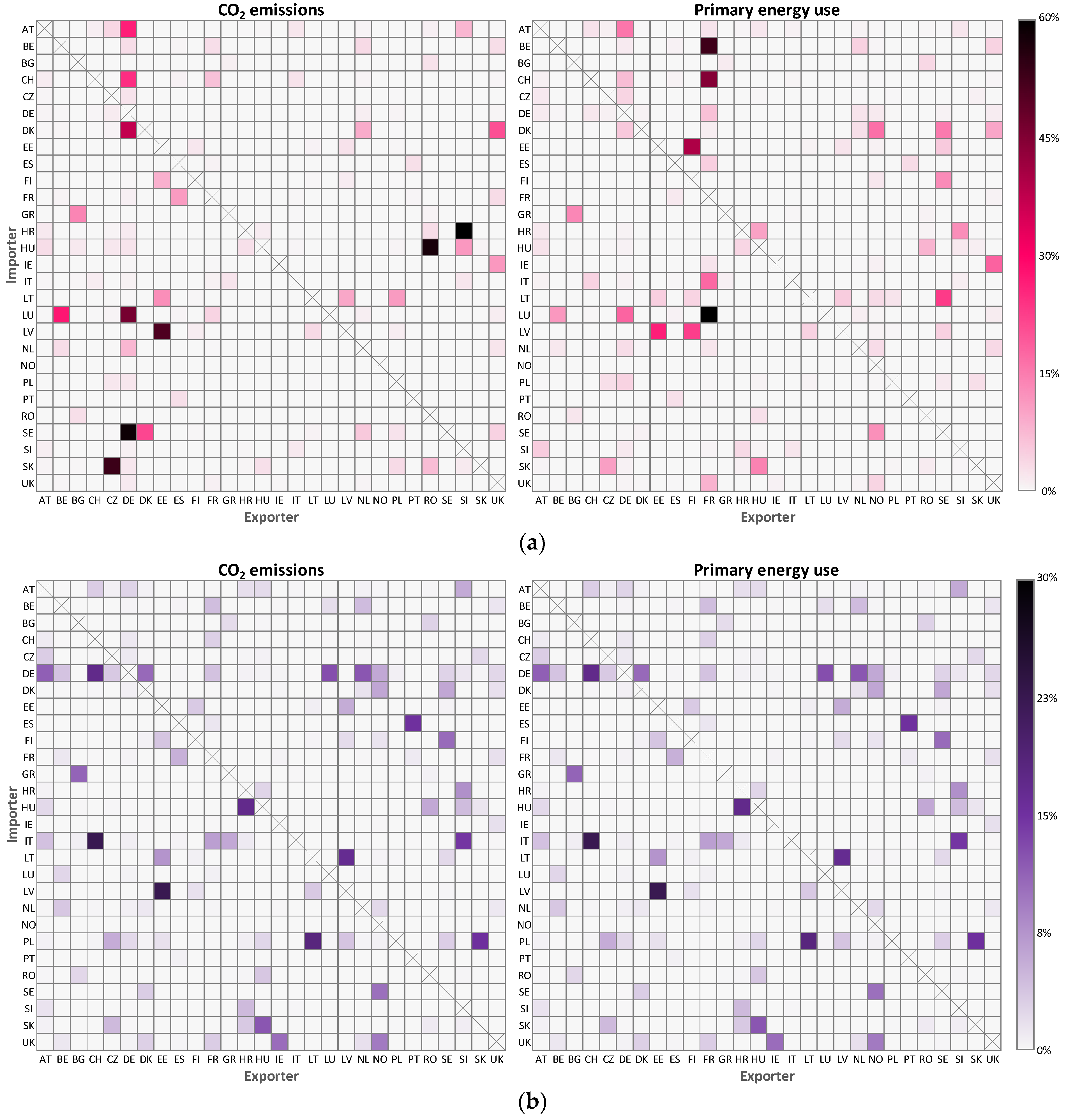
For every country, it is possible to calculate the total primary energy use and CO2 emissions that is associated with its electricity consumption—considering both the consumption of locally produced electricity as well as imported electricity. Based on these calculations, it is then possible to express for each country the fractions of these totals that were imported from other countries (Figure A2a). In terms of CO2 emissions, the NT.2030 results show that many of the countries surrounding Germany—which have relatively low CO2 intensities in terms of their own electricity production—import a significant share of their consumption-based CO2 emissions from Germany. Namely: Austria (26%), Switzerland (25%), Denmark (36%), Luxemburg (44%) and Sweden (54%). Similarly, many countries surrounding France—which themselves have a relatively low production-perspective PEF—import a considerable amount of their consumption-based primary energy use from France. Namely: Belgium (41%), Switzerland (37%), Italy (17%) and Luxembourg (44%).
Figure A2.
Total cross-country exchanges of CO2 and primary energy in the scenario-year NT.2030: (a) Imported CO2 emissions and primary energy use from a consumption perspective. Imported CO2 emissions and primary energy are expressed as a fraction of the total consumption-based CO2 emissions and primary energy of the importing country (respectively); (b) Exported CO2 emissions and primary energy use from a production perspective. Exported CO2 emissions and primary energy are expressed as a fraction of the total production-based CO2 emissions and primary energy of the exporting country (respectively).

Similarly, it is possible to calculate for every country the total CO2 emissions and primary energy use that is associated with its local electricity production. It is then possible to express for each country the fractions of these totals that were exported to other countries (Figure A2b). For example, Italy exports 22% of its production-based CO2 emissions to Switzerland, and Spain exports 15% of its production-based primary energy use to Portugal.
References
- European Commission. Stepping up Europe’s 2030 Climate Ambition Investing in a Climate-Neutral Future for the Benefit of Our People; European Commission: Brussels, Belgium, 2020. [Google Scholar]
- Marmiroli, B.; Messagie, M.; Dotelli, G.; Van Mierlo, J. Electricity Generation in LCA of Electric Vehicles: A Review. Appl. Sci. 2018, 8, 1384. [Google Scholar] [CrossRef] [Green Version]
- Moro, A.; Lonza, L. Electricity carbon intensity in European Member States: Impacts on GHG emissions of electric vehicles. Transp. Res. Part D Transp. Environ. 2018, 64, 5–14. [Google Scholar] [CrossRef] [PubMed]
- Eguiarte, O.; Garrido-Marijuán, A.; De Agustín-Camacho, P.; Del Portillo, L.; Romero-Amorrortu, A. Energy, Environmental and Economic Analysis of Air-to-Air Heat Pumps as an Alternative to Heating Electrification in Europe. Energies 2020, 13, 3939. [Google Scholar] [CrossRef]
- Azaza, M.; Eriksson, D.; Wallin, F. A study on the viability of an on-site combined heat- and power supply system with and without electricity storage for office building. Energy Convers. Manag. 2020, 213, 112807. [Google Scholar] [CrossRef]
- Ponstein, H.J.; Meyer-Aurich, A.; Prochnow, A. Greenhouse gas emissions and mitigation options for German wine production. J. Clean. Prod. 2019, 212, 800–809. [Google Scholar] [CrossRef]
- Schram, W.; Louwen, A.; Lampropoulos, I.; Van Sark, W. Comparison of the Greenhouse Gas Emission Reduction Potential of Energy Communities. Energies 2019, 12, 4440. [Google Scholar] [CrossRef] [Green Version]
- Lausselet, C.; Lund, K.; Brattebø, H. LCA and scenario analysis of a Norwegian net-zero GHG emission neighbourhood: The importance of mobility and surplus energy from PV technologies. Build. Environ. 2021, 189, 107528. [Google Scholar] [CrossRef]
- Reda, F.; Fatima, Z. Northern European nearly zero energy building concepts for apartment buildings using integrated solar technologies and dynamic occupancy profile: Focus on Finland and other Northern European countries. Appl. Energy 2019, 237, 598–617. [Google Scholar] [CrossRef]
- Niemelä, T.; Kosonen, R.; Jokisalo, J. Cost-effectiveness of energy performance renovation measures in Finnish brick apartment buildings. Energy Build. 2017, 137, 60–75. [Google Scholar] [CrossRef] [Green Version]
- Mata, É.; Wanemark, J.; Nik, V.M.; Kalagasidis, A.S. Economic feasibility of building retrofitting mitigation potentials: Climate change uncertainties for Swedish cities. Appl. Energy 2019, 242, 1022–1035. [Google Scholar] [CrossRef]
- D’Agostino, D.; Rossi, F.D.; Marino, C.; Minichiello, F.; Russo, F. Double plus-zero energy historic building and improvement of hygrothermal conditions for the Palaeontology Museum of Naples. J. Build. Phys. 2020. [Google Scholar] [CrossRef]
- Barrella, R.; Priego, I.; Linares, J.I.; Arenas, E.; Romero, J.C.; Centeno, E. Feasibility Study of a Centralised Electrically Driven Air Source Heat Pump Water Heater to Face Energy Poverty in Block Dwellings in Madrid (Spain). Energies 2020, 13, 2723. [Google Scholar] [CrossRef]
- Chen, X.; Qu, K.; Calautit, J.; Ekambaram, A.; Lu, W.; Fox, C.; Gan, G.; Riffat, S. Multi-criteria assessment approach for a residential building retrofit in Norway. Energy Build. 2020, 215, 109668. [Google Scholar] [CrossRef]
- Asim, M.; Saleem, S.; Imran, M.; Leung, M.K.H.; Hussain, S.A.; Miró, L.S.; Rodríguez, I. Thermo-economic and environmental analysis of integrating renewable energy sources in a district heating and cooling network. Energy Effic. 2019, 13, 79–100. [Google Scholar] [CrossRef]
- D’Agostino, D.; Parker, D.; Melià, P. Environmental and economic implications of energy efficiency in new residential buildings: A multi-criteria selection approach. Energy Strat. Rev. 2019, 26, 100412. [Google Scholar] [CrossRef]
- Las-Heras-Casas, J.; López-Ochoa, L.M.; López-González, L.M.; Olasolo-Alonso, P. Energy Renovation of Residential Buildings in Hot and Temperate Mediterranean Zones Using Optimized Thermal Envelope Insulation Thicknesses: The Case of Spain. Appl. Sci. 2021, 11, 370. [Google Scholar] [CrossRef]
- Munné-Collado, I.; Aprà, F.M.; Olivella-Rosell, P.; Villafáfila-Robles, R. The Potential Role of Flexibility during Peak Hours on Greenhouse Gas Emissions: A Life Cycle Assessment of Five Targeted National Electricity Grid Mixes. Energies 2019, 12, 4443. [Google Scholar] [CrossRef] [Green Version]
- Riboldi, L.; Völler, S.; Korpås, M.; Nord, L.O. An Integrated Assessment of the Environmental and Economic Impact of Offshore Oil Platform Electrification. Energies 2019, 12, 2114. [Google Scholar] [CrossRef] [Green Version]
- Barbu, M.; Darie, G.; Siroux, M. Analysis of a Residential Photovoltaic-Thermal (PVT) System in Two Similar Climate Conditions. Energies 2019, 12, 3595. [Google Scholar] [CrossRef] [Green Version]
- Calise, F.; Cappiello, F.L.; D’Accadia, M.D.; Vicidomini, M. Energy and economic analysis of a small hybrid solar-geothermal trigeneration system: A dynamic approach. Energy 2020, 208, 118295. [Google Scholar] [CrossRef]
- Ascione, F.; Bianco, N.; Rosa Francesca, D.M.; Mastellone, M.; Maria, G.; Peter, G. Energy & Buildings The role of the occupant behavior in affecting the feasibility of energy refurbishment of residential buildings: Typical effective retrofits compromised by typical wrong habits. Energy Build. 2020, 223, 110217. [Google Scholar] [CrossRef]
- Sobol, Ł.; Dyjakon, A. The Influence of Power Sources for Charging the Batteries of Electric Cars on CO2 Emissions during Daily Driving: A Case Study from Poland. Energies 2020, 13, 4267. [Google Scholar] [CrossRef]
- Jarre, M.; Noussan, M.; Simonetti, M. Primary energy consumption of heat pumps in high renewable share electricity mixes. Energy Convers. Manag. 2018, 171, 1339–1351. [Google Scholar] [CrossRef]
- Noussan, M.; Jarre, M.; Roberto, R.; Russolillo, D. Combined vs separate heat and power production—Primary energy comparison in high renewable share contexts. Appl. Energy 2018, 213, 1–10. [Google Scholar] [CrossRef]
- Noussan, M. Performance based approach for electricity generation in smart grids. Appl. Energy 2018, 220, 231–241. [Google Scholar] [CrossRef]
- Marrasso, E.; Roselli, C.; Sasso, M. Electric efficiency indicators and carbon dioxide emission factors for power generation by fossil and renewable energy sources on hourly basis. Energy Convers. Manag. 2019, 196, 1369–1384. [Google Scholar] [CrossRef]
- Neirotti, F.; Noussan, M.; Simonetti, M. Towards the electrification of buildings heating—Real heat pumps electricity mixes based on high resolution operational profiles. Energy 2020, 195, 116974. [Google Scholar] [CrossRef]
- Beloin-Saint-Pierre, D.; Padey, P.; Périsset, B.; Medici, V. Considering the dynamics of electricity demand and production for the environmental benchmark of Swiss residential buildings that exclusively use electricity. IOP Conf. Series: Earth Environ. Sci. 2019, 323, 012096. [Google Scholar] [CrossRef]
- Stinner, S.; Schlösser, T.; Huchtemann, K.; Müller, D.; Monti, A. Primary energy evaluation of heat pumps considering dynamic boundary conditions in the energy system. Energy 2017, 138, 60–78. [Google Scholar] [CrossRef]
- Bianco, V.; Scarpa, F.; Tagliafico, L.A. Estimation of primary energy savings by using heat pumps for heating purposes in the residential sector. Appl. Therm. Eng. 2017, 114, 938–947. [Google Scholar] [CrossRef]
- Hitchin, R. Primary Energy Factors and the primary energy intensity of delivered energy: An overview of possible calculation conventions. J. Build. Serv. Eng. Res. Technol. 2019, 40, 198–219. [Google Scholar] [CrossRef]
- Vandermeulen, A.; Vandeplas, L.; Patteeuw, D. Flexibility offered by residential floor heating in a smart grid context: The role of heat pumps and renewable energy sources in optimization towards different objectives. In Proceedings of the 12th IEA Heat Pump Conference 2017, Rotterdam, The Netherlands, 15–18 May 2017; pp. 1–12. [Google Scholar]
- González-Prieto, D.; Fernández-Nava, Y.; Marañón, E.; Prieto, M.M. Influence of Atlantic Microclimates in Northern Spain on the Environmental Performance of Lightweight Concrete Single-Family Houses. Energies 2020, 13, 4337. [Google Scholar] [CrossRef]
- Hirvonen, J.; Jokisalo, J.; Heljo, J.; Kosonen, R. Towards the EU emissions targets of 2050: Optimal energy renovation measures of Finnish apartment buildings. Int. J. Sustain. Energy 2019, 38, 649–672. [Google Scholar] [CrossRef] [Green Version]
- Bastida-Molina, P.; Hurtado-Pérez, E.; Peñalvo-López, E.; Cristina, E.; Moros-Gómez, M.C. Assessing transport emissions reduction while increasing electric vehicles and renewable generation levels. Transp. Res. Part D Transp. Environ. 2020, 88, 102560. [Google Scholar] [CrossRef]
- Lausselet, C.; Borgnes, V.; Brattebø, H. LCA modelling for Zero Emission Neighbourhoods in early stage planning. Build. Environ. 2019, 149, 379–389. [Google Scholar] [CrossRef]
- Merzkirch, A.; Maas, S.; Scholzen, F.; Waldmann, D. Primary energy used in centralised and decentralised ventilation systems measured in field tests in residential buildings. Int. J. Vent. 2019, 18, 19–27. [Google Scholar] [CrossRef]
- Piccardo, C.; Dodoo, A.; Gustavsson, L.; Tettey, U. Retrofitting with different building materials: Life-cycle primary energy implications. Energy 2020, 192, 116648. [Google Scholar] [CrossRef]
- Sowa, J.; Mijakowski, M. Humidity-Sensitive, Demand-Controlled Ventilation Applied to Multiunit Residential Building—Performance and Energy Consumption in Dfb Continental Climate. Energies 2020, 13, 6669. [Google Scholar] [CrossRef]
- Küfeoğlu, S.; Hong, D.K.K. Emissions performance of electric vehicles: A case study from the United Kingdom. Appl. Energy 2020, 260, 114241. [Google Scholar] [CrossRef]
- Huber, J.; Lohmann, K.; Schmidt, M.; Weinhardt, C. Carbon efficient smart charging using forecasts of marginal emission factors. J. Clean. Prod. 2021, 284, 124766. [Google Scholar] [CrossRef]
- Grijalva, E.R.; Martínez, J.M.L. Analysis of the Reduction of CO2 Emissions in Urban Environments by Replacing Conventional City Buses by Electric Bus Fleets: Spain Case Study. Energies 2019, 12, 525. [Google Scholar] [CrossRef] [Green Version]
- Pinel, D.; Korpås, M.; Lindberg, K.B. Impact of the CO2 factor of electricity and the external CO2 compensation price on zero emission neighborhoods’ energy system design. Build. Environ. 2021, 187, 107418. [Google Scholar] [CrossRef]
- Peppas, A.; Kollias, K.; Politis, A.; Karalis, L.; Taxiarchou, M.; Paspaliaris, I. Performance evaluation and life cycle analysis of RES-hydrogen hybrid energy system for office building. Int. J. Hydrog. Energy 2021, 46, 6286–6298. [Google Scholar] [CrossRef]
- Leerbeck, K.; Bacher, P.; Junker, R.G.; Tveit, A.; Corradi, O.; Madsen, H.; Ebrahimy, R. Control of Heat Pumps with CO2 Emission Intensity Forecasts. Energies 2020, 13, 2851. [Google Scholar] [CrossRef]
- Dixon, J.; Bukhsh, W.; Edmunds, C.; Bell, K. Scheduling electric vehicle charging to minimise carbon emissions and wind curtailment. Renew. Energy 2020, 161, 1072–1091. [Google Scholar] [CrossRef]
- Pina, E.A.; Lozano, M.A.; Serra, L.M.; Hernández, A.; Lázaro, A. Design and thermoeconomic analysis of a solar parabolic trough—ORC—Biomass cooling plant for a commercial center. Sol. Energy 2021, 215, 92–107. [Google Scholar] [CrossRef]
- Clauß, J.; Stinner, S.; Solli, C.; Lindberg, K.B.; Madsen, H.; Georges, L. Evaluation Method for the Hourly Average CO2eq. Intensity of the Electricity Mix and Its Application to the Demand Response of Residential Heating. Energies 2019, 12, 1345. [Google Scholar] [CrossRef] [Green Version]
- Bellocchi, S.; Klöckner, K.; Manno, M.; Noussan, M.; Vellini, M. On the role of electric vehicles towards low-carbon energy systems: Italy and Germany in comparison. Appl. Energy 2019, 255, 113848. [Google Scholar] [CrossRef]
- Petrovic, B.; Myhren, J.A.; Zhang, X.; Wallhagen, M.; Eriksson, O. Life cycle assessment of a wooden single-family house in Sweden. Appl. Energy 2019, 251, 113253. [Google Scholar] [CrossRef]
- Ballarini, I.; De Luca, G.; Paragamyan, A.; Pellegrino, A.; Corrado, V. Transformation of an Office Building into a Nearly Zero Energy Building (nZEB): Implications for Thermal and Visual Comfort and Energy Performance. Energies 2019, 12, 895. [Google Scholar] [CrossRef] [Green Version]
- Pedersen, T.H.; Hedegaard, R.E.; Petersen, S. Space heating demand response potential of retrofitted residential apartment blocks. Energy Build. 2017, 141, 158–166. [Google Scholar] [CrossRef]
- ENTSO-E. TYNDP 2020—Scenario Report. 2020. Available online: https://2020.entsos-tyndp-scenarios.eu/ (accessed on 6 March 2021).
- Eurelectric. Power Barometer 2020. 2020. Available online: https://www.eurelectric.org/power-barometer/ (accessed on 6 March 2021).
- Ringkjøb, H.-K.; Haugan, P.M.; Solbrekke, I.M. A review of modelling tools for energy and electricity systems with large shares of variable renewables. Renew. Sustain. Energy Rev. 2018, 96, 440–459. [Google Scholar] [CrossRef]
- ENTSO-E. TYNDP 2020—Scenario Building Guidelines (Methodology Report). 2020. Available online: https://2020.entsos-tyndp-scenarios.eu/ (accessed on 6 March 2021).
- ENTSO-E. TYNDP 2020 Annex 1—Further Assumptions on the Ambition Tool. 2020. Available online: https://2020.entsos-tyndp-scenarios.eu/ (accessed on 6 March 2021).
- Brodny, J.; Tutak, M. Analyzing Similarities between the European Union Countries in Terms of the Structure and Volume of Energy Production from Renewable Energy Sources. Energies 2020, 13, 913. [Google Scholar] [CrossRef] [Green Version]
- ENTSO-E. Mid-Term Adequacy Forecast 2020—Appendix 2: Methodology. 2020. Available online: https://2020.entsos-tyndp-scenarios.eu/ (accessed on 6 March 2021).
- Hörsch, J.; Schäfer, M.; Becker, S.; Schramm, S.; Greiner, M. Flow tracing as a tool set for the analysis of networked large-scale renewable electricity systems. Int. J. Electr. Power Energy Syst. 2018, 96, 390–397. [Google Scholar] [CrossRef] [Green Version]
- Tranberg, B.; Schafer, M.; Brown, T.; Horsch, J.; Greiner, M. Flow-Based Analysis of Storage Usage in a Low-Carbon European Electricity Scenario. In Proceedings of the 2018 15th International Conference on the European Energy Market (EEM), Lodz, Poland, 27–29 June 2018. [Google Scholar] [CrossRef] [Green Version]
- Tranberg, B.; Corradi, O.; Lajoie, B.; Gibon, T.; Staffell, I.; Andresen, G.B. Real-time carbon accounting method for the European electricity markets. Energy Strat. Rev. 2019, 26, 100367. [Google Scholar] [CrossRef]
- Schafer, M.; Tranberg, B.; Jones, D.; Weidlich, A. Tracing carbon dioxide emissions in the European electricity markets. In Proceedings of the 2020 17th International Conference on the European Energy Market (EEM), Stockholm, Sweden, 16–18 September 2020. [Google Scholar]
- De Chalendar, J.A.; Taggart, J.; Benson, S.M. Tracking emissions in the US electricity system. Proc. Natl. Acad. Sci. USA 2019, 116, 25497–25502. [Google Scholar] [CrossRef] [Green Version]
- Esser, A.; Sensfuss, F. Evaluation of Primary Energy Factor Calculation Options for Electricity; Fraunhofer-Institute für System-und Innovationsforschung (ISI): Karlsruhe, Germany, 2016. [Google Scholar]
- Ensslen, A.; Schücking, M.; Jochem, P.; Steffens, H.; Fichtner, W.; Wollersheim, O.; Stella, K. Empirical carbon dioxide emissions of electric vehicles in a French-German commuter fleet test. J. Clean. Prod. 2017, 142, 263–278. [Google Scholar] [CrossRef] [Green Version]
- Hall, M.; Geissler, A. Different balancing methods for Net Zero Energy Buildings—Impact of time steps, grid interaction and weighting factors. Energy Procedia 2017, 122, 379–384. [Google Scholar] [CrossRef]
- Noussan, M.; Roberto, R.; Nastasi, B. Performance Indicators of Electricity Generation at Country Level—The Case of Italy. Energies 2018, 11, 650. [Google Scholar] [CrossRef] [Green Version]
- Holland, S.P.; Mansur, E.T.; Muller, N.Z.; Yates, A.J. Are There Environmental Benefits from Driving Electric Vehicles? The Importance of Local Factors. Am. Econ. Rev. 2016, 106, 3700–3729. [Google Scholar] [CrossRef] [Green Version]
- Hamels, S.; Himpe, E.; Laverge, J.; Delghust, M.; Van den, M.; Brande KV, D.; Janssens, A.; Albrecht, J. The use of primary energy factors and CO2 intensities—Reviewing the state of play in academic literature (preprint). arXiv 2020, arXiv:abs/2102.13539. [Google Scholar]
- Lidberg, T.; Gustafsson, M.; Myhren, J.; Olofsson, T.; Trygg, L.Ö. Former Environmental impact of energy refurbishment of buildings within different district heating systems. Appl. Energy 2018, 227, 231–238. [Google Scholar] [CrossRef]
- Alavijeh, N.M.; Steen, D.; Norwood, Z.; Tuan, L.A.; Agathokleous, C. Cost-Effectiveness of Carbon Emission Abatement Strategies for a Local Multi-Energy System—A Case Study of Chalmers University of Technology Campus. Energies 2020, 13, 1626. [Google Scholar] [CrossRef] [Green Version]
- Tutak, M.; Brodny, J.; Siwiec, D.; Ulewicz, R.; Bindzár, P. Studying the Level of Sustainable Energy Development of the European Union Countries and Their Similarity Based on the Economic and Demographic Potential. Energies 2020, 13, 6643. [Google Scholar] [CrossRef]
- Collins, S.; Deane, J.; Gallachóir, B.Ó. Adding value to EU energy policy analysis using a multi-model approach with an EU-28 electricity dispatch model. Energy 2017, 130, 433–447. [Google Scholar] [CrossRef]
- Deane, J.; Driscoll, A.; Gallachóir, B.Ó. Quantifying the impacts of national renewable electricity ambitions using a North–West European electricity market model. Renew. Energy 2015, 80, 604–609. [Google Scholar] [CrossRef]
- Collins, S.; Deane, P.; OGallachoir, B.; Pfenninger, S.; Staffell, I. Impacts of Inter-Annual Wind and Solar Variations on the European Power System Impacts of Inter-Annual Wind and Solar Variations on the European Power System. Joule 2018, 2, 2076–2090. [Google Scholar] [CrossRef] [Green Version]
- Collins, S.; Deane, J.P.; Poncelet, K.; Panos, E.; Pietzcker, R.C.; Delarue, E.; Gallachóir, B.P.Ó. Integrating short term variations of the power system into integrated energy system models: A methodological review. Renew. Sustain. Energy Rev. 2017, 76, 839–856. [Google Scholar] [CrossRef] [Green Version]
- Deane, J.; Drayton, G.; Gallachóir, B.P.Ó. The impact of sub-hourly modelling in power systems with significant levels of renewable generation. Appl. Energy 2014, 113, 152–158. [Google Scholar] [CrossRef]
- Welsch, M.; Deane, P.; Howells, M.; Gallachóir, B.Ó.; Rogan, F.; Bazilian, M.; Rogner, H.-H. Incorporating flexibility requirements into long-term energy system models—A case study on high levels of renewable electricity penetration in Ireland. Appl. Energy 2014, 135, 600–615. [Google Scholar] [CrossRef]
- Deane, J.; Chiodi, A.; Gargiulo, M.; Gallachóir, B.P.Ó. Soft-linking of a power systems model to an energy systems model. Energy 2012, 42, 303–312. [Google Scholar] [CrossRef]
- Drayton, G.; McCoy, M.; Pereira, M.; Cazalet, E.; Johannis, M.; Phillips, D. Transmission expansion planning in the western interconnection—The planning process and the analytical tools that will be needed to do the job. In Proceedings of the IEEE PES Power Systems Conference and Exposition, New York, NY, USA, 10–13 October 2004; pp. 1–6. [Google Scholar] [CrossRef]
- Nweke, C.I.; Leanez, F.; Drayton, G.R.; Kolhe, M. Benefits of chronological optimization in capacity planning for electricity markets. In Proceedings of the 2012 IEEE International Conference on Power System Technology (POWERCON), Auckland, New Zealand, 23–26 October 2012; pp. 1–6. [Google Scholar] [CrossRef]
- Hobbs, B.F.; Bartholomew, E.; Chen, Y.; Drayton, G.; Lise, W. Improved Transmission Representations in Oligopolistic Market Models. In Proceedings of the 2006 IEEE PES Power Systems Conference and Exposition, Atlanta, GA, USA, 29 October–1 November 2006; Volume 23, pp. 81–86. [Google Scholar] [CrossRef]
- Deane, J.; Gracceva, F.; Chiodi, A.; Gargiulo, M.; Gallachóir, B.P. Assessing power system security. A framework and a multi model approach. Int. J. Electr. Power Energy Syst. 2015, 73, 283–297. [Google Scholar] [CrossRef]
- Deane, J.; Ciaráin, M.Ó.; Gallachóir, B.Ó. An integrated gas and electricity model of the EU energy system to examine supply interruptions. Appl. Energy 2017, 193, 479–490. [Google Scholar] [CrossRef]
- Foley, A.; Tyther, B.; Calnan, P.; Gallachóir, B.Ó. Impacts of Electric Vehicle charging under electricity market operations. Appl. Energy 2013, 101, 93–102. [Google Scholar] [CrossRef]
- Gil, E.; Aravena, I. Evaluating the contribution of intermittent generation to power system adequacy at different demand levels. In Proceedings of the 2013 IEEE Power & Energy Society General Meeting, Vancouver, BC, Canada, 21–25 July 2013; pp. 1–5. [Google Scholar] [CrossRef]
- Gil, E.; Aravena, I.; Cardenas, R. Generation Capacity Expansion Planning Under Hydro Uncertainty Using Stochastic Mixed Integer Programming and Scenario Reduction. IEEE Trans. Power Syst. 2014, 30, 1838–1847. [Google Scholar] [CrossRef]
- Ibanez, E.; Magee, T.; Clement, M.; Brinkman, G.; Milligan, M.; Zagona, E. Enhancing hydropower modeling in variable generation integration studies. Energy 2014, 74, 518–528. [Google Scholar] [CrossRef] [Green Version]
- Shirley, R.; Kammen, D. Energy planning and development in Malaysian Borneo: Assessing the benefits of distributed technologies versus large scale energy mega-projects. Energy Strat. Rev. 2015, 8, 15–29. [Google Scholar] [CrossRef]
- Gaffney, F.; Deane, J.P.; Drayton, G.; Glynn, J.; Gallachóir, B.P.Ó. Comparing negative emissions and high renewable scenarios for the European power system. BMC Energy 2020, 2, 1–13. [Google Scholar] [CrossRef]
Figure 1.
Structural overview of the methodology, results, and discussion.

Figure 2.
Geographical scope of the unit commitment economic dispatch (UCED) model. Dotted lines represent transmission connections that are not (yet) built in every scenario-year. Cross-border exchanges with the surrounding area (e.g., Russia, Turkey and the non-EU countries in the Balkan region) are neglected, given the fact they are responsible for less than 1% of electricity consumed in the modelled region [55].

Figure 3.
Overview of the methodological steps from the UCED model and the flow-tracing technique to the calculated hourly conversion factors, showing a ten-day period for Belgium in the scenario-year NT.2030: (a) Electricity generation, imports and exports; (b) imports, exports, and net imports; (c) flow-traced disaggregation of net imports; (d) hourly CO2 intensity (kg/MWh) and PEF (MWhp/MWhe), both from a production and consumption perspective, and (in the case of PEF) showing values for both the considered calculation methodologies.


Figure 4.
Nodal balance of physical electricity flows.

Figure 5.
Evolution of yearly conversion factor values across the seven scenario-years: (a) CO2 intensities; (b) primary energy factors (PEFs).
Figure 5.
Evolution of yearly conversion factor values across the seven scenario-years: (a) CO2 intensities; (b) primary energy factors (PEFs).

Figure 6.
Duration curves of average hourly conversion factors for each of the seven scenario-years: (a) CO2 intensities; (b) Primary energy factors (PEFs).
Figure 6.
Duration curves of average hourly conversion factors for each of the seven scenario-years: (a) CO2 intensities; (b) Primary energy factors (PEFs).

Figure 7.
Electricity generation mix in winter and summer.

Figure 8.
Imports and exports in winter and summer. To improve comparability across countries, cumulative amounts of (net) import and export are expressed as a share of cumulative demand in the respective period.
Figure 8.
Imports and exports in winter and summer. To improve comparability across countries, cumulative amounts of (net) import and export are expressed as a share of cumulative demand in the respective period.

Figure 9.
Distribution of hourly conversion factor values in winter and summer periods. Countries are grouped according to relative values, to optimize comparability across 2025 and 2040. Bottom grey = P5–P25, colored area = P25–P75, top grey = P75–P95, white dot = average value: (a) CO2 intensities; (b) primary energy factors (PEFs).

Figure 10.
Distribution of hourly conversion factors as a function of (residual) load. In the case of residual load, negative values can occur. Namely when the cumulative generation of wind and solar technologies is higher than the hourly load. Excess renewable generation is typically exported, or curtailed if necessary.

Figure 11.
Distribution of hourly conversion factors across the 24h daily cycle. Bottom grey = P5–P25, green area = P25–P75, top grey = P75–P95, black dot = average value.
Figure 11.
Distribution of hourly conversion factors across the 24h daily cycle. Bottom grey = P5–P25, green area = P25–P75, top grey = P75–P95, black dot = average value.

Figure 12.
Impact of taking into account imports on yearly average conversion factors (a) CO2 intensities; (b) primary energy factors (PEFs).
Figure 12.
Impact of taking into account imports on yearly average conversion factors (a) CO2 intensities; (b) primary energy factors (PEFs).

Figure 13.
Difference in PEF hourly values depending on the assumed PEF for hydro, wind and solar. Bottom grey = P5–P25, colored area = P25–P75, top grey = P75–P95, white dot = average value.
Figure 13.
Difference in PEF hourly values depending on the assumed PEF for hydro, wind and solar. Bottom grey = P5–P25, colored area = P25–P75, top grey = P75–P95, white dot = average value.

Figure 14.
Duration curves of marginal hourly conversion factors for each of the seven scenario-years (a) CO2 intensities; (b) primary energy factors (PEFs).
Figure 14.
Duration curves of marginal hourly conversion factors for each of the seven scenario-years (a) CO2 intensities; (b) primary energy factors (PEFs).

Table 3.
CO2 intensities and primary energy factors per technology.
| Technology | CO2 Intensity (kg/MWh) | PEF (MWhp/MWhe) |
|---|---|---|
| Nuclear | 0 | 3.0 |
| Gas CCGT new | 342 | 1.7 |
| Gas CCGT old 1 | 513 | 2.5 |
| Gas CCGT old 2 | 428 | 2.1 |
| Gas CCGT present 1 | 366 | 1.8 |
| Gas CCGT present 2 | 354 | 1.7 |
| Gas conventional old 1 | 570 | 2.8 |
| Gas conventional old 2 | 500 | 2.4 |
| Gas OCGT new | 489 | 2.4 |
| Gas OCGT old | 586 | 2.9 |
| Hard coal new | 736 | 2.2 |
| Hard coal old 1 | 967 | 2.9 |
| Hard coal old 2 | 846 | 2.5 |
| Lignite new | 790 | 2.2 |
| Lignite old 1 | 1039 | 2.9 |
| Lignite old 2 | 909 | 2.5 |
| Heavy oil old 1 | 802 | 2.9 |
| Heavy oil old 2 | 702 | 2.5 |
| Light oil | 802 | 2.9 |
| Oil shale new | 923 | 2.6 |
| Oil shale old | 1241 | 3.4 |
| Solar, wind, hydro | 0 | 0 or 1 |
Note: The values for every technology remain constant across the simulated scenarios and timeframes (e.g., 2025, 2030 and 2040), with the exception of the CO2 intensities of gas technologies. These are lower in the “Distributed Energy” and “Global Ambition” scenarios [57]. For example, “Gas CCGT new” has a CO2 intensity of 300 kg/MWh in the year 2030, and 157 kg/MWh in the year 2040. This reflects the partial use of low-carbon gas, which is included in the storylines of these scenarios.
Publisher’s Note: MDPI stays neutral with regard to jurisdictional claims in published maps and institutional affiliations. |
© 2021 by the author. Licensee MDPI, Basel, Switzerland. This article is an open access article distributed under the terms and conditions of the Creative Commons Attribution (CC BY) license (https://creativecommons.org/licenses/by/4.0/).
Share and Cite
MDPI and ACS Style
Hamels, S. CO2 Intensities and Primary Energy Factors in the Future European Electricity System. Energies 2021, 14, 2165. https://0-doi-org.brum.beds.ac.uk/10.3390/en14082165
AMA Style
Hamels S. CO2 Intensities and Primary Energy Factors in the Future European Electricity System. Energies. 2021; 14(8):2165. https://0-doi-org.brum.beds.ac.uk/10.3390/en14082165
Chicago/Turabian StyleHamels, Sam. 2021. "CO2 Intensities and Primary Energy Factors in the Future European Electricity System" Energies 14, no. 8: 2165. https://0-doi-org.brum.beds.ac.uk/10.3390/en14082165
Note that from the first issue of 2016, this journal uses article numbers instead of page numbers. See further details here.