Optimal Individual Phase Voltage Regulation Strategies in Active Distribution Networks with High PV Penetration Using the Sparrow Search Algorithm

Abstract

This study aimed to propose individual phase voltage regulation strategies using the sparrow search algorithm (SSA) in the IEEE 8500-node large-scale unbalanced distribution network with high photovoltaic (PV) penetration. The proposed approach is capable of individual phase regulation, which coordinates the on-load tap changer (OLTC), voltage regulator (VR), switched capacitor bank (SCB), and volt–var setting controlled by a smart inverter to improve voltage variation and unbalance. Consequently, the change time of VRs, the switched times of SCBs, and the individual phase voltage magnitude and unbalance ratio are considered in the fitness function for the SSA. The simulation scenarios fully consider the unbalanced load conditions and PV power output patterns, and the numerical results demonstrate that the voltage variation and unbalance are clearly improved, by 15% and 26%, respectively. The fitness values, operation times of OLTC, VR, and SCB, and the settings of the volt–var controlled smart inverter are also optimized by the SSA. The outcomes of this study are helpful for distribution system operators in formulating voltage control strategies corresponding to different system conditions.

1. Introduction

The use of renewable energy increased by 3% in 2020 as the global demand for other fossil fuels decreased, consistent with 7% growth in electricity power generation from renewable energy resources, such as wind turbine and photovoltaic (PV) sources [1]. Renewable energy resources currently play an important role in power system planning, operation, and control, and will continue to do so in the future. Among the vertical structures of power systems in Taiwan, the large-scale wind and PV farms, which have an installation capacity of nearly 20 MW, are interconnected in transmission or sub-transmission networks. The other relatively small systems are in distribution networks (DNs); capacity of less than 10 MW is installed in 22.8 kV primary feeders, and capacity of less than 5 MW is installed in 11.4 kV primary feeders. A capacity less than 2 MW is also installed in secondary low-voltage conductors. The Taiwanese government has declared that 20 GW PV will be installed until 2025. In 2021, PV installation capacity accounted for around 40% of the total 49.77 GW installed capacity. Consequently, the intermittence of PV effects of DNs cannot be ignored because it results in voltage quality problems [2,3,4,5,6], such as voltage fluctuation, overvoltage, voltage sag, voltage dip, and unbalanced voltage. Related studies have proposed feasible techniques and solutions to overcome these problems [7,8,9,10,11,12,13].

Oh et al. [14] proposed a dynamic network reconfiguration approach, which uses cooperation to control the power output fluctuations of distributed renewable energy resources (DRERs) in DNs with high penetration of DRERs. Li et al. [15] introduced and applied several novel metamodel-based global optimization methods to minimize network voltage deviation and power loss in optimal operation of active DNs. A real power capping method was proposed to maintain voltage profiles, continuously maximize PV generation, and evenly distribute the real power curtailments among all PV systems by adaptively setting the power caps for PV inverters in real time to prevent overvoltage in DNs with high penetration of PV [16]. A probabilistic optimal strategy was also proposed in [17] to minimize voltage deviation by utilizing PV generators as capacitors and inductors to compensate for reactive power in coordination with a substation transformer on-load tap changer (OLTC). Chamana and Chowdhury [18] presented a zone-based multistage time-graded operation of voltage regulators (VRs), capacitor banks, and OLTC transformers to regulate voltage in unbalanced DNs with high penetration of PV. To simultaneously solve voltage regulation and unbalance caused by high penetration of PV, Gerdroodbari et al. [19] proposed a reactive power-based control strategy for single-phase PV inverters. This approach used two algorithms based on communication links between PV inverters to exchange information. A real-time approach was also designed to coordinate PV inverters and a battery energy storage system for voltage regulation. This method can compensate for fast voltage fluctuations of PV power in each control cycle of 5 s [20]. Similarly, Zhang et al. [21] applied a battery energy storage system for fast, smooth, and flexible voltage control in an interconnected industrial feeder with highly distributed energy resources. To address the voltage fluctuations caused by the high penetration of DRERs in DNs, an optimal capacity allocation strategy of energy storage system was proposed in [22], and the coordination of active and reactive power of DRERs and energy storage systems has also been proposed for optimal operations [23,24]. The application of energy storage systems achieves better performance compared to traditional techniques, such as OLTC, VR, and SCB; however, these systems are not currently economic. The voltage quality problem is relative to the hosting capacity of DRERs in DNs [25,26,27]. Thus, a novel input–process–output stochastic–probabilistic conductor size selection framework was proposed for distribution feeders with DRERs to determine the sizing of conductors for future loading conditions considering DRER allocation uncertainty [25]. From the related literature mentioned above, the proposed method, objective function, and control strategy or device for voltage regulation caused by high PV penetration in DNs are listed in

Table 1. The proposed method, objective function, and control strategy/device of related literature.

Reference	Method	Objective Function	Control Strategy/Devices
[14]	Short-term operational method	Minimizing the number of switching operations and power curtailment	Voltage control, network reconfiguration, and power curtailment
[15]	Metamodel-based global optimization methods	Minimize network voltage deviation and power loss	Dispatch distributed generators and energy storage systems
[16]	Real power capping method	Fairly distributing the real power curtailments	Setting the power caps for PV inverters
[17]	Probabilistic optimal strategy	Minimize voltage deviation	Utilizing PV generators as capacitors and inductors and coordinate with substation transformer on-load tap changer (OLTC)
[18]	Multistage volt–var optimization algorithm	Minimize the curtailment of PV inverter output	Control voltage regulators, capacitor banks, and OLTC transformers to regulate voltage
[19]	Reactive power-based control strategy	Improve voltage unbalance and voltage regulation	Communication links between PV inverters to exchange information
[20]	real-time method	compensate fast voltage fluctuations	Coordinate step voltage regulator, PV inverter and battery energy storage system
[21,22,23,24]	Sensitivity-based voltage control strategy, optimal capacity allocation strategy, and mathematical programing model	Minimize voltage fluctuations and mitigate voltage unbalance	Battery energy storage system

.

According to the related research issues discussed in this paper, the high penetration of PV in DNs largely affects the voltage quality problem. Consequently, coordination of the operation times of OLTC, VR, and SCB, and the settings of the volt–var controlled smart inverter, constitute the primary task in addressing the complicated optimal combination problem. In particular, in unbalanced distribution networks, the individual phase regulation strategies are essential. Therefore, a metaheuristic-based method, which is distinct from the abovementioned works, is proposed for individual phase voltage regulation strategies considering the objective function and corresponding constraints. The details are described in the following sections.

2. Benefit and Challenge of Smart Inverter Volt-Var Control in DNs

At present, a grid-tie inverter of PVs with active and reactive power control, which is called a smart inverter, is universally used in power utilities and PV plants. The outstanding ability of volt–var control of voltage regulation solves the problem derived from the intermittent nature of PV output. The benefits of the smart inverter in DNs are illustrated in this section, and the objective functions of the optimization problem in this study are formulated on the basis of these benefits. Moreover, the challenge of the volt–var control setting formulation is considered for the algorithm constraint.

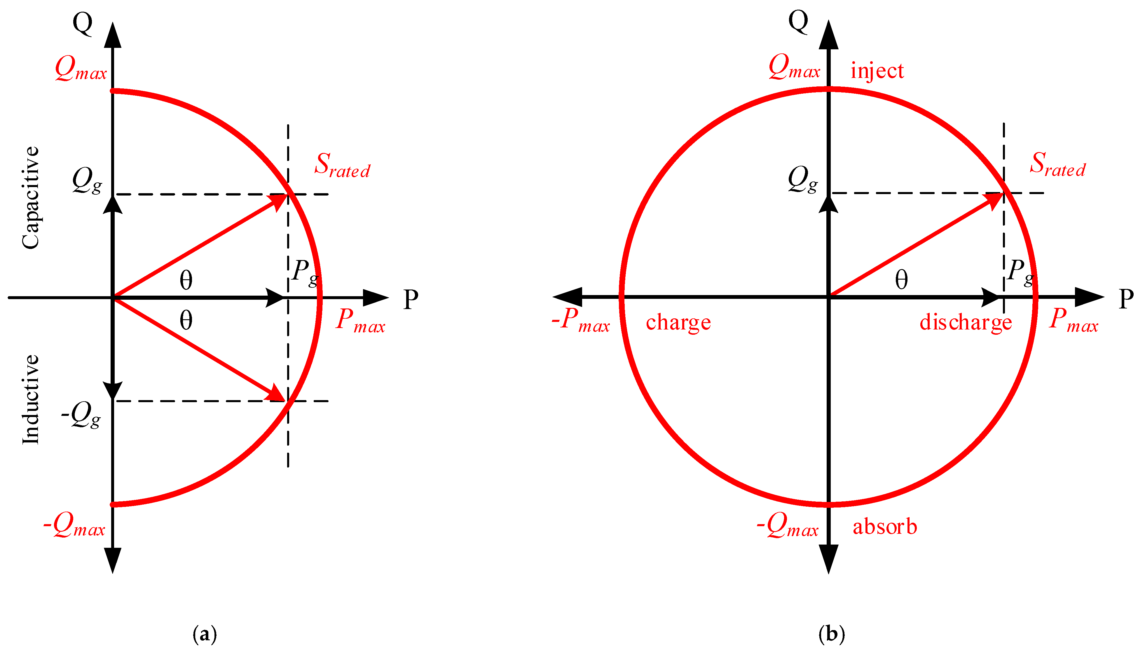
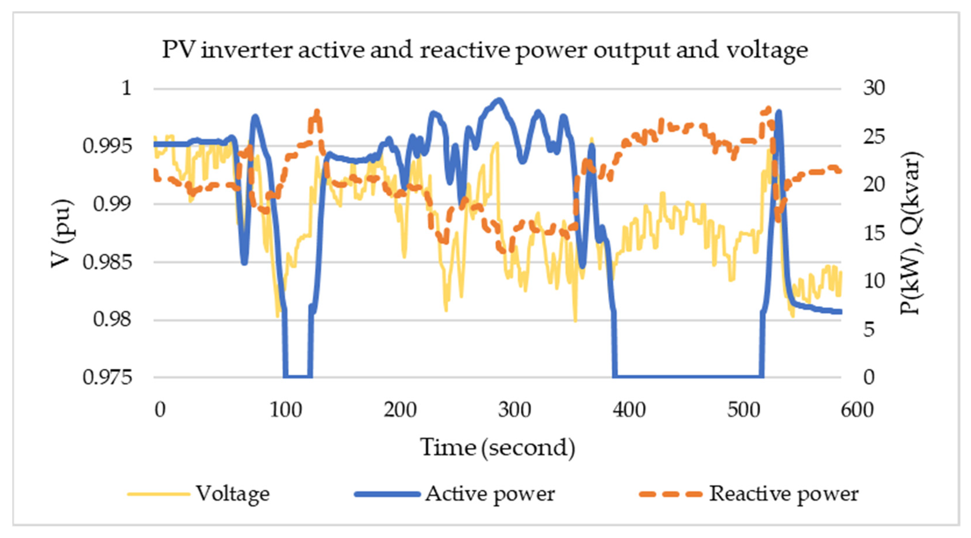
2.1. Function of Smart Inverter

A smart inverter is an AC/DC power electronic element that can flexibly control the injection of active power (P, unit W), and inductive and capacitive reactive power (Q, unit var) into the power grid. Smart inverters have the capability to output inductive or capacitive reactive power that is the same as the rated apparent power (S, unit VA). The capability curve of the PV smart inverter is shown in Figure 1a. As observed, its power factor (PF) leads or lags $\cos \theta =\frac{P_g}{S_{rated}}$, and P_g represents the injection or absorption of the active power of the smart inverter. Furthermore, the bidirectional inverter of the battery energy storage system (BESS), which is also named the power conditioning system, can simultaneously inject or absorb active and reactive power. Thus, its four-quadrant operation capability curve is shown in Figure 1b. As a result of its flexible output ability, several functions of smart inverters have been developed, such as fixed-Q mode, fixed-PF mode, V-Q (volt–var) mode, V-P (volt–watt) mode, and F-P (frequency–watt) mode. Different control modes are operated depending on distinct demands or scenarios of the system.

2.2. Volt–Var Control for Voltage Variation Reduction

For power grids with high PV penetration, the active power output may decrease suddenly due to weather issues, such as solar radiation, clouds, rain, and poor visibility. The grid voltage sag arises according to Equation (1):

$$\mathrm{\Delta }V\approx \mathrm{\Delta }P\times R+\mathrm{\Delta }Q\times X,$$

(1)

where R is the resistance and X is the reactance of the conductor. Fortunately, the smart inverter has the capability to output capacitive reactive power to mitigate the voltage sag, as shown in Figure 2, when the active power drops. Relatively, inductive reactive power mitigates the voltage swell, which is the so-called V-Q control or volt–var control. The X/R ratio in DNs is usually under 3, whereas the R is nearly ignored in power transmission systems due to the large X. Thus, the volt–var control significantly benefits the voltage regulation in transmission systems. Consequently, volt–var control of the smart inverter plays an important role in voltage regulation in power grids with high PV penetration, and its flexibility also increases the effectiveness. Voltage regulation in DNs can be attained using OLTC and VRs, which are autotransformers with a tap range of 10%. In the long-distance feeder, the VRs are utilized to increase end voltage by installing them on the middle section of the feeder. The operation of the PV smart inverter can reduce the number of changes in tap position due to the fast response and flexible reactive power output ability. Some switched capacitor banks (SCBs) are used to avoid the undervoltage in DNs, and the switching times are also reduced by the volt–var control. Moreover, the grid-tie PV of kW or MW level is generally integrated by a number of inverters individually controlled by phase, which means the three-phase voltage unbalance can be improved.

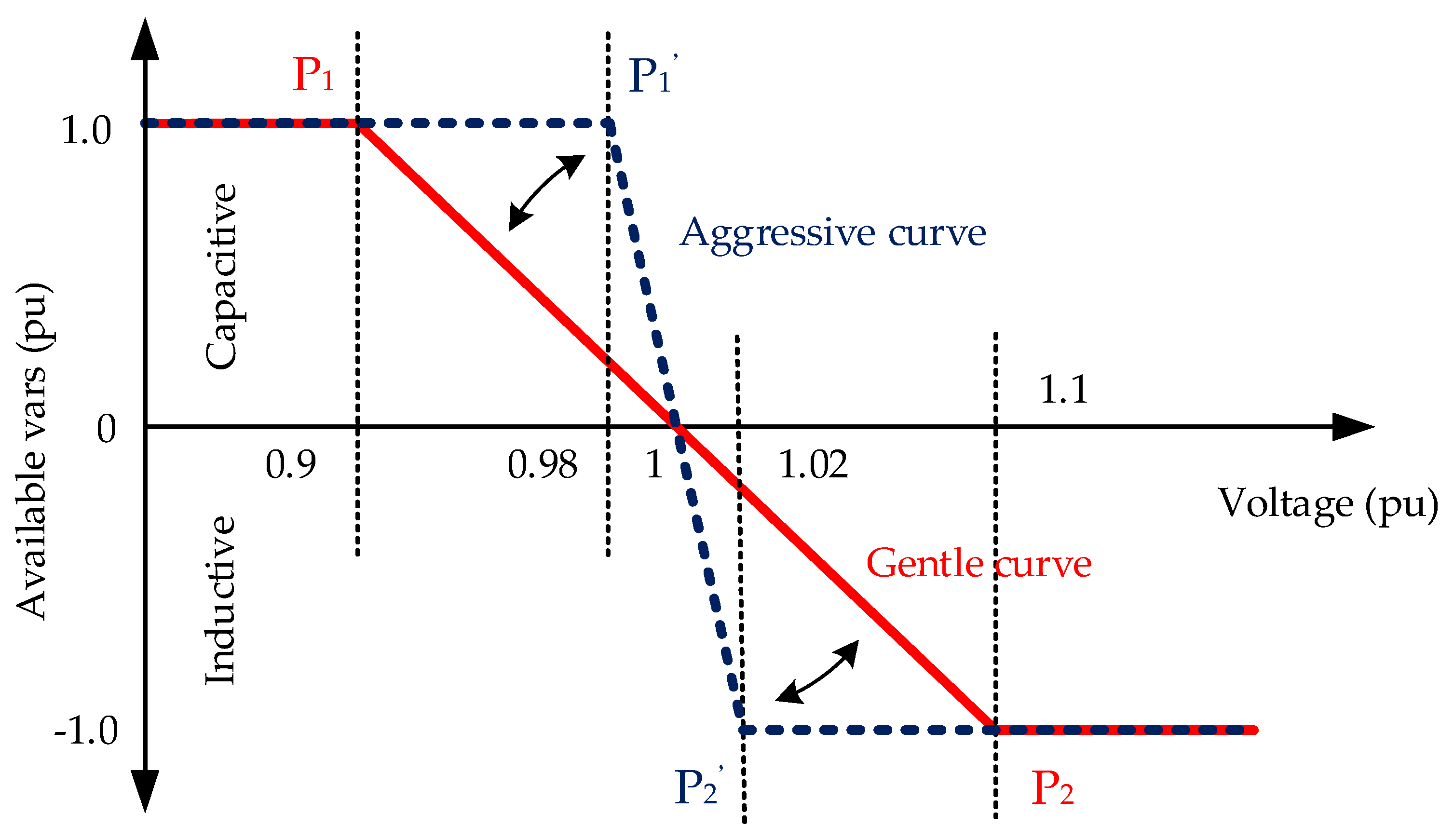
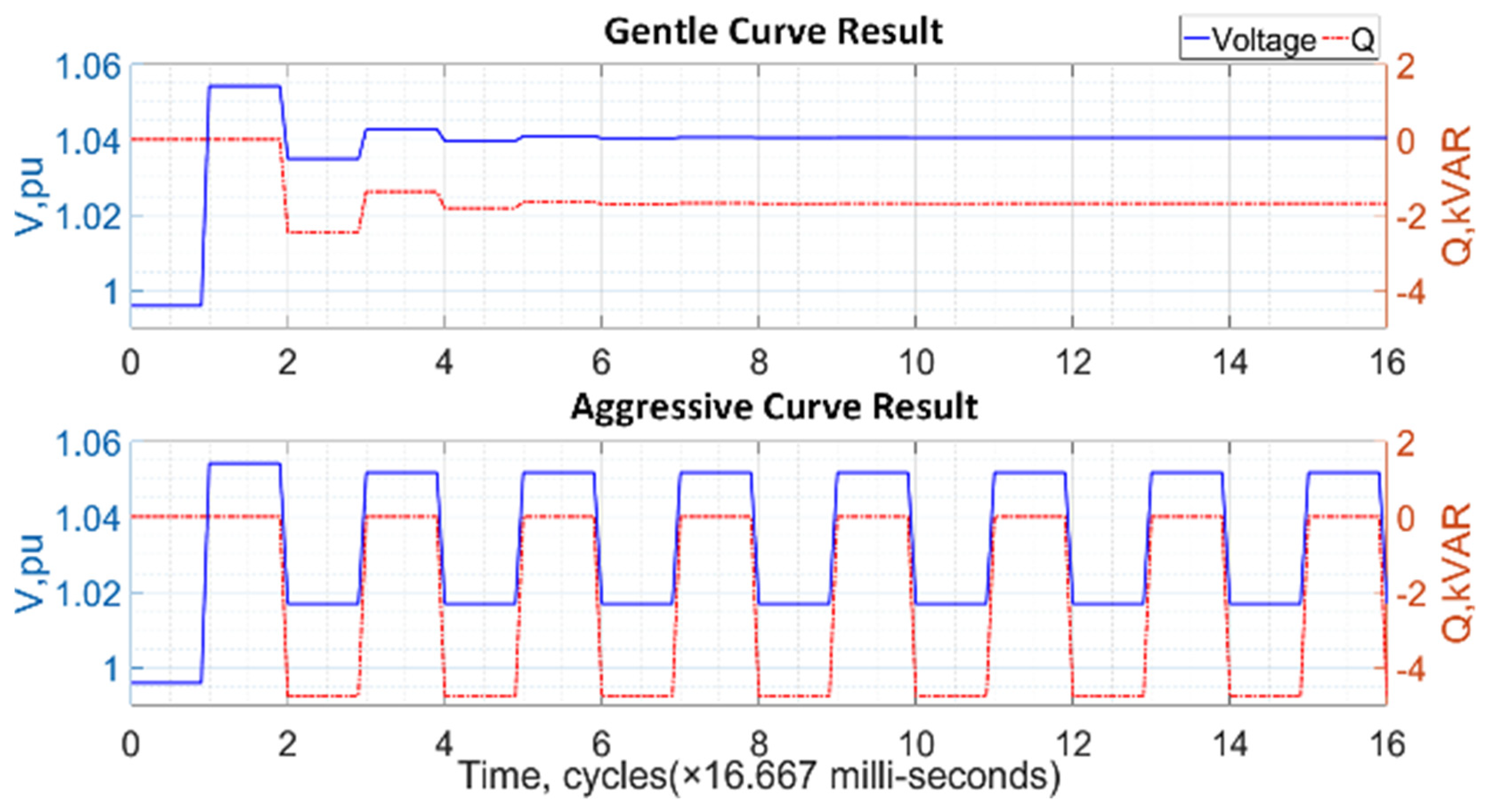
2.3. Volt-Var Control Curve Setting

The control mode of the smart inverter, and the volt–var control curve, depends on the scenario. The slope and deadband of the control curve impact the response of the reactive power output. Figure 3 shows the two control curves, which are labeled gentle and aggressive curves. The aggressive curve with a steep slope can regulate voltage faster. However, it may result in the oscillation of voltage and reactive power, as shown in Figure 4, according to [28]. By contrast, the gentle curve controls the voltage smoothly, but its voltage regulation ability is worse than that of the aggressive curve. Therefore, it is necessary to carefully consider the control curve setting in formulating a voltage control strategy using volt–var control of the PV smart inverter. Moreover, it is important to leverage between the gentle and aggressive curves based on the PV rated capacity and impedance of the point of common coupling.

3. Sample System and Problem Description

In this study, the volt–var control setting of the PV smart inverters distributed in the IEEE 8500-node test system were optimized using the SSA. The sample system, optimization problems, objective function, and constraints of the algorithm are described in this section.

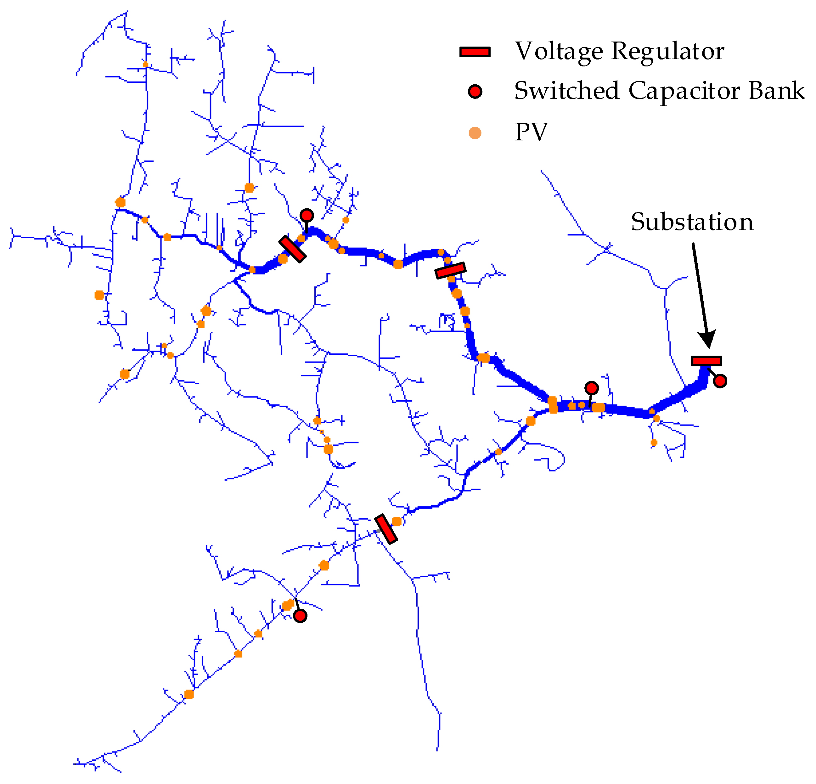
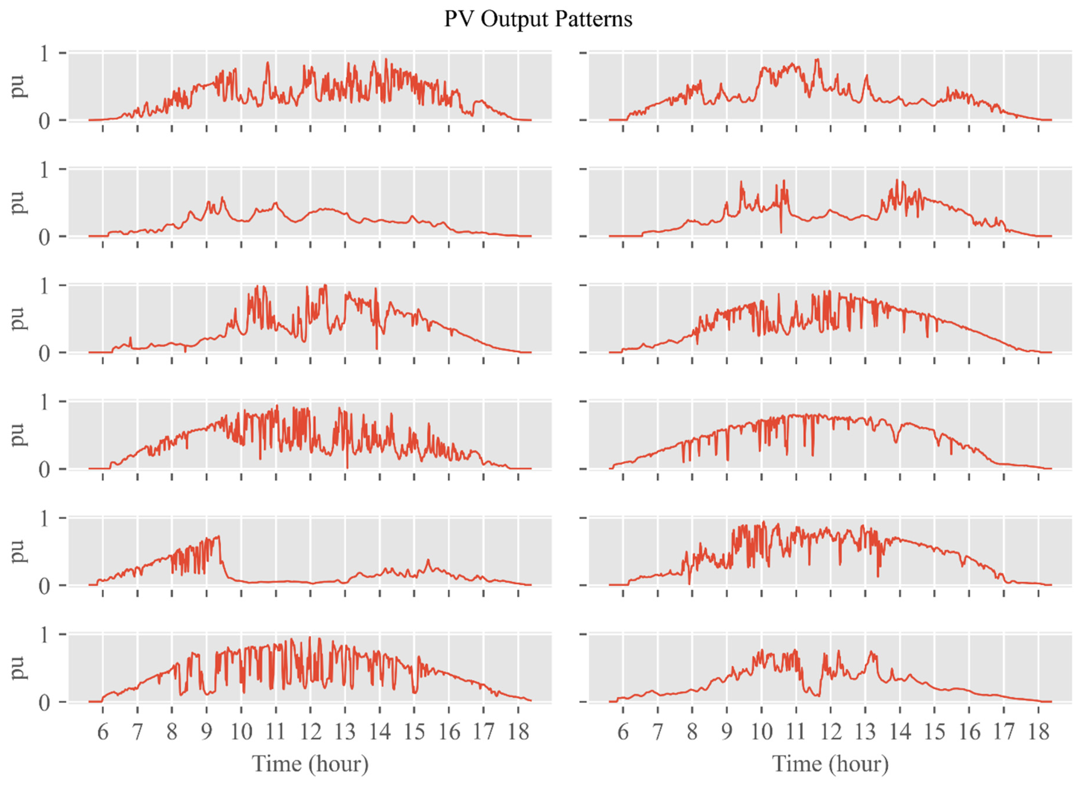
3.1. Sample DNs and Simulation Scenarios

The IEEE 8500-node test feeder was used in this study as the sample system. The single-line diagram, which was plotted using the OpenDSS engine, is shown in Figure 5. This system includes 8500 nodes, four VRs, and four SCBs. The total unbalanced load of the system is approximately 12,000 kVA. PV installation of 8887 kW was assumed by the authors to be distributed over the feeder main, and the distribution energy resource penetration rate is nearly 74%. This high PV penetration simulates the effects of each setting of volt–var control in the PV smart inverter. Given the long distance of the IEEE 8500-node test feeder, several voltage regulation devices are used to avoid voltage violation in the middle or end sections of the feeder, such as VRs and SCBs. An OLTC having 32 steps is in the distribution substation of the 115 kV/12.47 kV main transformer of two windings, three VRs are in the middle section of the feeder, one SCB is installed in the substation, and three SCBs are in middle section of the feeder. All of the devices are individual phase controlled, and the control feedback is the installation bus voltage.

The positions of the PVs, VRs, and SCBs are marked in Figure 5. The larger circle represents the larger capacity of the PV, and the wider line indicates larger power congestion of the branch. The power flow was calculated using the OpenDSS engine in this study. VR control, capacitor control, and inverter control models with strategies that can be defined by the user are considered in the engine. Furthermore, each PV plant has different power output patterns, as shown in Figure 6, to enhance the diversity of the simulation and closely replicate the actual situation. The simulation period is 766 min during the day, from about 5:40 to 18:20. The optimization problem of this study is to coordinate the volt–var control settings of points P1 and P2 in Figure 3 of all the PV smart inverters. The different reactive power outputs are expected to have different effects on the distribution system. The optimization objective is illustrated in the next subsection.

3.2. Objective Functions

The volt–var control setting points of each PV smart inverter in this study were optimized using the proposed method, and the voltage variation and profile were thus improved. The three-phase voltage unbalance can also be mitigated to reduce the neutral current and total line loss due to the individual phase control. Moreover, the mitigation of voltage variation reduces the operation times of voltage regulation devices, such as VRs and SCBs. Accordingly, the voltage profile is smoother and the power quality is improved. Therefore, the objective functions are described as follows for the algorithm to search for the best solution to the abovementioned problems:

$$fi{t}^1=\left({\displaystyle \sum _{i=1}^N{\displaystyle \sum _{t=0}^T\left|\frac{V_{t+1}^i-V_t^i}{V_t^i}\right|\times 100\%}}\right)/N\times T,$$

(2)

where $V_t^i$ is the voltage at the ith bus in the tth second; N denotes the bus number and T is the number of the time point. Thus, Equation (2) is the average voltage variation of each bus in all the simulation periods.

$$fi{t}^2=\underset{t,i}{\max }\left(\left|\frac{V_{t+1}^i-V_t^i}{V_t^i}\right|\times 100\%\right),$$

(3)

Equation (3) is the maximum voltage variation of each bus in all the simulation periods.

$$fi{t}^3=\left(\underset{t,i}{\max }\left(V_t^i\right)-1\right)/0.03+\left(1-\underset{t,i}{\min }\left(V_t^i\right)\right)/0.05,$$

(4)

Equation (4) represents the maximum and minimum voltage deviations of each bus in all the simulation periods with a voltage of 1 pu. Considering the voltage violation in grid code (1.03 pu for overvoltage and 0.95 pu for undervoltage), the deviation is normalized by dividing by 0.03 and 0.05.

$$fi{t}^4=\left({\displaystyle \sum _{i=1}^N{\displaystyle \sum _{t=0}^T\frac{V_{0,t}^i}{V_{1,t}^i}\times 100\%}}\right)/N\times T+\left({\displaystyle \sum _{i=1}^N{\displaystyle \sum _{t=0}^T\frac{V_{2,t}^i}{V_{1,t}^i}\times 100\%}}\right)/N\times T,$$

(5)

where $V_{0,t}^i$, $V_{1,t}^i$, and $V_{2,t}^i$ are the zero-, positive-, and negative-sequence voltages at the ith bus in the tth second. Thus, $\frac{V_{0,t}^i}{V_{1,t}^i}$ and $\frac{V_{2,t}^i}{V_{1,t}^i}$ are the zero- and negative-sequence voltage unbalance. Accordingly, Equation (5) is the average zero-sequence voltage unbalance plus the average negative-sequence voltage unbalance of each bus in all the simulation periods.

$$fi{t}^5=\underset{t,i}{\max }\left(\frac{V_{0.t}^i}{V_{1,t}^i}\times 100\%\right)+\underset{t,i}{\max }\left(\frac{V_{2.t}^i}{V_{1,t}^i}\times 100\%\right),$$

(6)

Equation (6) is the maximum zero-sequence voltage unbalance plus the maximum negative-sequence voltage unbalance of each bus in all the simulation periods.

$$fi{t}^6={\displaystyle \sum _{k=1}^K{N}_{VR}^k}+{\displaystyle \sum _{i=1}^L{N}_{SCB}^l},$$

(7)

where $N_{SVR}^k$ represents the number of tap changes of the kth VR; $N_{SCB}^l$ represents the switching times of the lth SCB in the test feeder during the simulation period.

The bus voltage variation and maximum and minimum voltage deviations are optimized together to satisfy the grid code. Thus, the objective function is expressed in Equation (8):

$$fi{t}^7=fi{t}^1+fi{t}^2+fi{t}^3$$

(8)

Moreover, voltage unbalances are optimized together to improve three-phase unbalance. Thus, the objective function is expressed in Equation (9):

$$fi{t}^8=fi{t}^4+fi{t}^5$$

(9)

3.3. Constraints

As mentioned in Section 2.3, the aggressive curve of the volt–var control setting can be used to obtain a better voltage profile. However, it can result in unacceptable sustained voltage oscillation. The magnitude of oscillation is reflected by different PV capacity values and Thevenin’s equivalent impedance on each location of the PV. The optimization algorithm is constrained by the number of iterations of the inverter control algorithm in the OpenDSS engine to prevent the oscillation problem. The maximum number of iterations is set to 150. If it is exceeded, then the voltage oscillation is regarded to be too large to be accepted.

Furthermore, the voltage variation limit of the grid code is $\pm 3\%$, and the overvoltage and undervoltage are 0.95 and 1.03, respectively. In the solution procedure, the magnitude of bus voltage in the feeder main is limited between 0.95 and 1.03, and in each regulation time step, the voltage variation percentage is limited to less than or equal to 3%. Thus, the optimization algorithm must be subjected to the following constraints:

$$0.95\le V_t^i\le 1.03,$$

(10)

$$\left|\frac{V_{t+1}^i-V_t^i}{V_t^i}\times 100\%\right|\le 3\%$$

(11)

4. Proposed Approach and Solution Framework

The different setting points of each smart inverter distributed in the test feeder generate a large number of solutions. A metaheuristic with high calculation speed and good global search capability is a good choice to solve this complicated problem. This section illustrates the algorithm and software framework chosen in this study.

4.1. Metaheuristic Algorithm

A metaheuristic is suitable for solving the optimization problem in DNs. The complicated and varied planning problems of DNs are difficult to define. Although a metaheuristic uses simple mathematics, it can search all of the possible solutions. Users only need to define the upper bounds, lower bounds, and dimensions of the problem, and set the number of populations and number of iterations. Most problem solutions can be searched using this mechanism. Several types of metaheuristic are inspired by different systems, such as evolutionary-based, swarm-based, physics-based, human-based, and bio-based approaches. The swarm-based types are usually good at global searching in the solution space and use simple mathematical equations, enabling fast calculation.

Twenty-five popular swarm-based metaheuristics were investigated and tested using a benchmark function, namely, the Rosenbrock function, as shown in Equation (12), where $x=\left(x_i,\dots ,x_N\right)\in {ℝ}^N$, N is its dimension, and the global minimum is 0. This was undertaken to determine the most suitable algorithm for the optimization problem in this study. Given that the dimension of the optimization problem of volt–var control settings is 360 (60 PVs × 3 phases × 2 setting points), the dimension of the benchmark function is also 360, and the numbers of populations and iterations are equal to 50.

Table 2. The performance of popular swarm-based metaheuristics.

Number	Algorithm	Solution	Calculation Time (s)
1	Particle Swarm Optimization	500.4533	1.763311
2	Bacterial Foraging Optimization	1881.848	161.7007
3	Cat Swarm Optimization	1616.839	16.95562
4	Artificial Bee Colony	1687.319	2.31785
5	Fireworks Algorithm	874.7588	6.671301
6	Bat Algorithm	125.4193	1.734487
7	Social Spider Optimization	41.2206	2.118863
8	Grey Wolf Optimizer	6.393672	1.664644
9	Social Spider Algorithm	24.93394	1.769286
10	Ant Lion Optimizer	100.0107	14.05951
11	Moth Flame Optimization	2203.492	1.706515
12	Elephant Herding Optimization	18.83527	1.852681
13	Whale Optimization Algorithm	2.861351	1.783804
14	Bird Swarm Algorithm	14.53802	1.678526
15	Spotted Hyena Optimizer	213.2286	3.040973
16	Swarm Robotics Search And Rescue	228.944	3.718125
17	Grasshopper Optimisation Algorithm	493.2859	3.931606
18	Moth Search Algorithm	2014.994	0.896199
19	Nake Mole-rat Algorithm	14.59282	1.693511
20	Bald Eagle Search	14.50522	4.956734
21	Pathfinder Algorithm	14.56558	3.901061
22 * 3	Sailfish Optimizer	2.92 × 10−8	17.08235
23 * 2	Harris Hawks Optimization	0.002945	1.496736
24	Manta Ray Foraging Optimization	14.46316	3.267328
25 * 1	Sparrow Search Algorithm	5.34 × 10−6	1.846647

* Denote the top three ranking algorithms.

lists the performance of each swarm-based metaheuristic, in terms of solution (0 is the correct solution) and calculation time. For the problem having a dimension of 360, population size of 50, and 50 iterations, most swarm-based metaheuristics cannot converge around the best solution. Only the Sailfish Optimizer (SO), Harris Hawks Optimization (HHO), and the Sparrow Search Algorithm (SSA) find solutions near 0. Of these, the SSA obtains the best solution and requires less time than SO. Thus, the SSA was chosen to be the optimization algorithm in this work.

$$f\left(x\right)={\displaystyle \sum _{i=1}^{N-1}\left[100{\left(x_{i+1}-x_i^2\right)}^2+{\left(1-x_i\right)}^2\right]}$$

(12)

4.2. Sparrow Search Algorithm

The SSA [29] was proposed by Xue and Shen in 2020. It is inspired by group wisdom, foraging, and anti-predation behavior of the captive house sparrow. The sparrow swarm has producers and scroungers. The producers actively search for the food source, whereas the scroungers obtain food through the producers. The producers and scroungers can flexibly switch between each other for the foraging strategy. However, their proportion must be unchanged in the whole population. Sparrows that are close to a rich food source, which represents a better fitness value and has higher energy, act by following the procedure. Several starving scroungers are more likely to fly to another place for food to gain more energy. Furthermore, once sparrows detect a predator, they begin to rise an alarm signal. The producers then need to lead all the scroungers to a safe area until the alarm value is greater than the safety threshold.

The producers are responsible for searching for food and guiding the movements of the scroungers. Thus, they are good at global searching. The location of the producers is updated as follows:

$$X_{i,j}^{t+1}=\{\begin{array}{ll}{X}_{i,j}^t\cdot \exp \left(\frac{-i}{\alpha \cdot T}\right)& if R_2<ST\\ X_{i,j}^t+Q\cdot L& if R_2\ge ST\end{array},$$

(13)

where t indicates the current iteration; ${\mathrm{X}}_{i,j}^t$, having dimension of 1 × d, represents the matrix of the jth dimension of the ith sparrow in iteration t. T is the number of iterations. $\alpha \in [0, 1]$ is a random number. $R_2\in [0, 1]$ and $ST\in [0.5, 1]$ represent the alarm value and safety threshold, respectively. Q is a random number which obeys a normal distribution. L shows a matrix of 1 × d for which each element inside is 1.

When scroungers know that a producer has found good food, they immediately fly to that producer to compete for the food; otherwise, they continue to monitor the producers. Therefore, the scrounger is good at searching for the local best solution. The location of the scroungers is updated as follows:

$$X_{i,j}^{t+1}=\{\begin{array}{cc}Q\cdot \exp \left(\frac{X_{i,j}^t-X_{worst}^t}{i^2}\right)\hfill & \hfill if i>\frac{n}{2}\\ X_P^{t+1}+\left|X_{i,j}^t-X_P^{t+1}\right|\cdot A^{+}\cdot L \hfill & \hfill \mathit{\text{otherwise}}\end{array},$$

(14)

where $X_P$ is the optimal position occupied by the producer, and $X_{worst}$ denotes the current global worst location. $A$ represents a matrix of 1 × d for which each element inside is randomly assigned a value of 1 or −1, and $A^{+}=A^T{(A{A}^T)}^{-1}$. When $i>\frac{n}{2}$, the ith scrounger with the worse fitness value is most likely to be starving.

A total of 10% to 20% of the population of the sparrow swarm is aware of the danger. These sparrows quickly move toward the safe area, whereas the sparrows in the middle of the group randomly walk to be close to others. The mathematical model can be expressed as follows:

$$X_{i,j}^{t+1}=\{\begin{array}{ll}{X}_{best}^t+\beta \cdot \left|X_{i,j}^t-X_{best}^t\right|& if f_i<f_g\\ X_{i,j}^t+K\cdot \left(\frac{\left|X_{i,j}^t-X_{worst}^t\right|}{\left(f_i-f_w\right)+\epsilon }\right)& if f_i=f_g\end{array},$$

(15)

where $X_{best}$ is the current global optimal location. $\beta$, as the step size control parameter, is a normal distribution of random numbers with a mean value of 0 and a variance of 1. $K\in [-1, 1]$ is a random number. Here, $f_i$ is the fitness value of the present sparrow. $f_g$ and $f_w$ are the current global best and worst fitness values, respectively. $\epsilon$ is the smallest constant to avoid a zero-division error.

Due to the three behaviors of the sparrow, which are responsible for global searching, local searching, and avoiding poor solutions, the algorithm converges quickly in a problem of large dimensions having small populations and a small number of iterations. Thus, the volt–var control setting optimization can be accurately solved using the SSA. The details of the SSA are provided in [29].

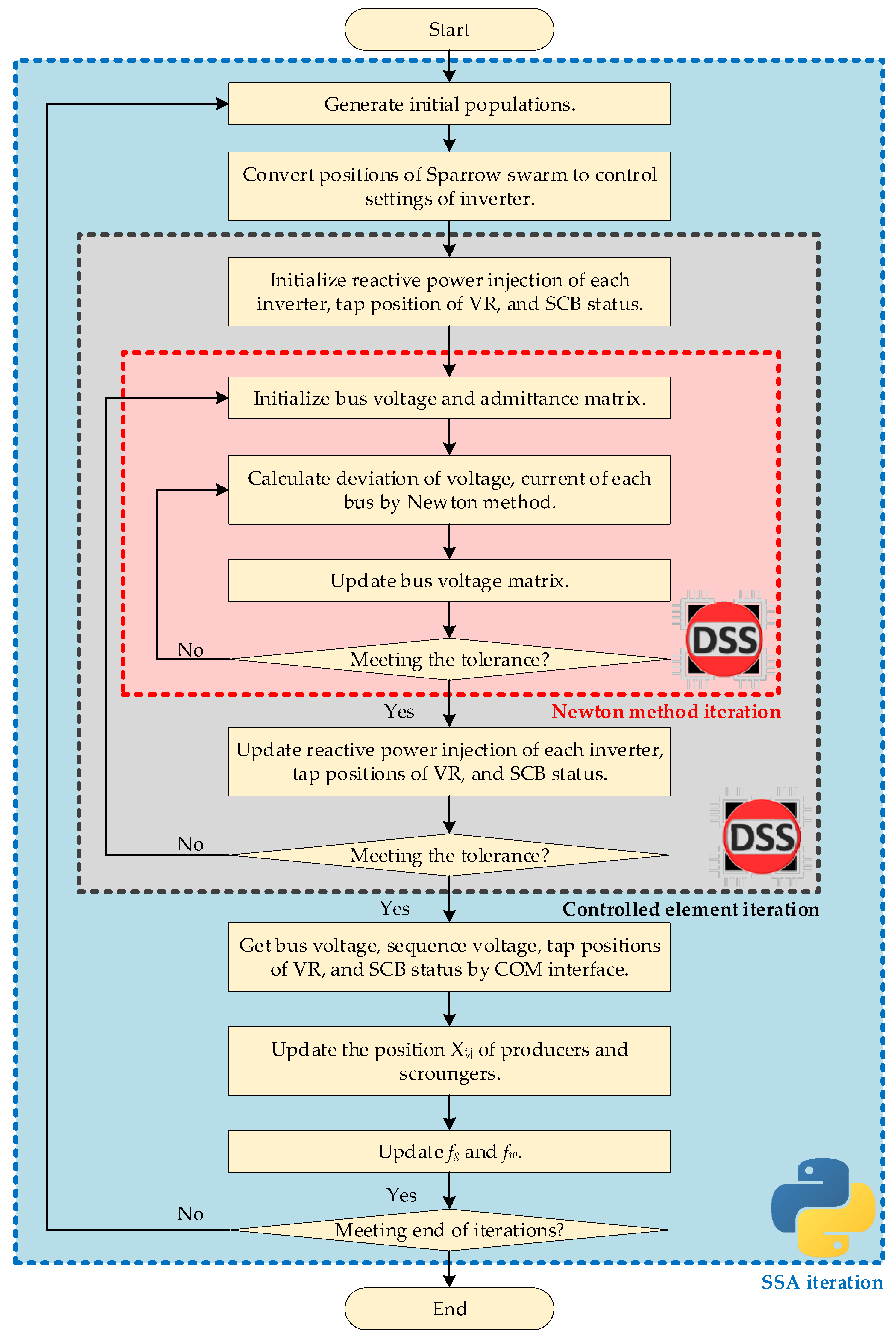
4.3. Solution Framework

The SSA in this work was coded in the Python language, and the IEEE 8500-node test system was established by an Electric Power Research Institute official in the OpenDSS engine. The volt–var control settings were modified using Python through a COM interface according to the sparrow positions in the SSA. Then, the OpenDSS engine calculated the bus voltage, branch current, sequence voltage, loss, tap positions of VR, and SCB status. Finally, it delivered the outcomes to Python.

Figure 7 shows the flowchart of the optimization solution framework in this study. It can be divided into three iterative processes: Newton method iteration, controlled element iteration, and SSA iteration. First, the SSA generates the initial population of the sparrow swarm and converts the sparrows’ positions to the control setting of the smart inverters. Second, to calculate the fitness value of the SSA, OpenDSS derives the power flow using the Newton method and repeatedly updates the smart inverter reactive power injection, tap positions of VR, and SCB status until convergence. Thus, three iterative processes are considered in the Python and OpenDSS environment. The processes in OpenDSS require the most calculation time because of the continuous power flow solution and control element iteration during the period of 766 min. Thus, a metaheuristic for small populations and a small number of iterations must be chosen.

5. Numerical Results and Discussion

The outcomes of the volt–var control optimization algorithm are presented in this section, including the objective functions mentioned above, such as voltage variation, three-phase voltage unbalance, tap positions of VR, and SCB status. In this paper, boxplots are used to illustrate the bus voltage spread of the simulation results; the interquartile range represents the data between 25% and 75%, and outliers are observations that are numerically distant from the remainder of the data, e.g., 1.5 times outside the interquartile range (above the upper quartile or below the lower quartile).

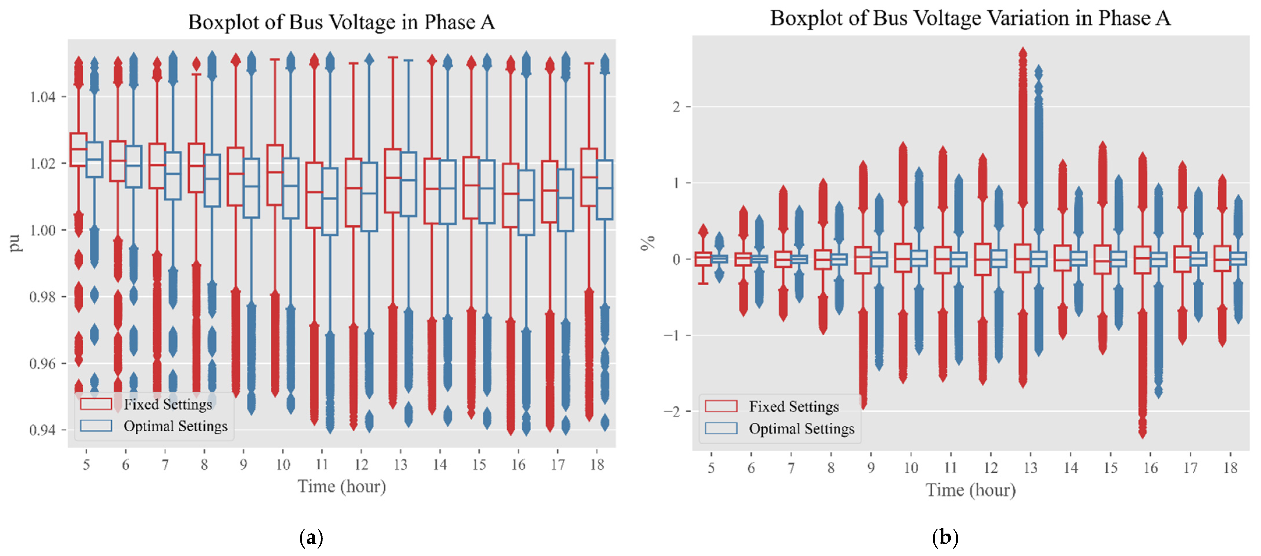
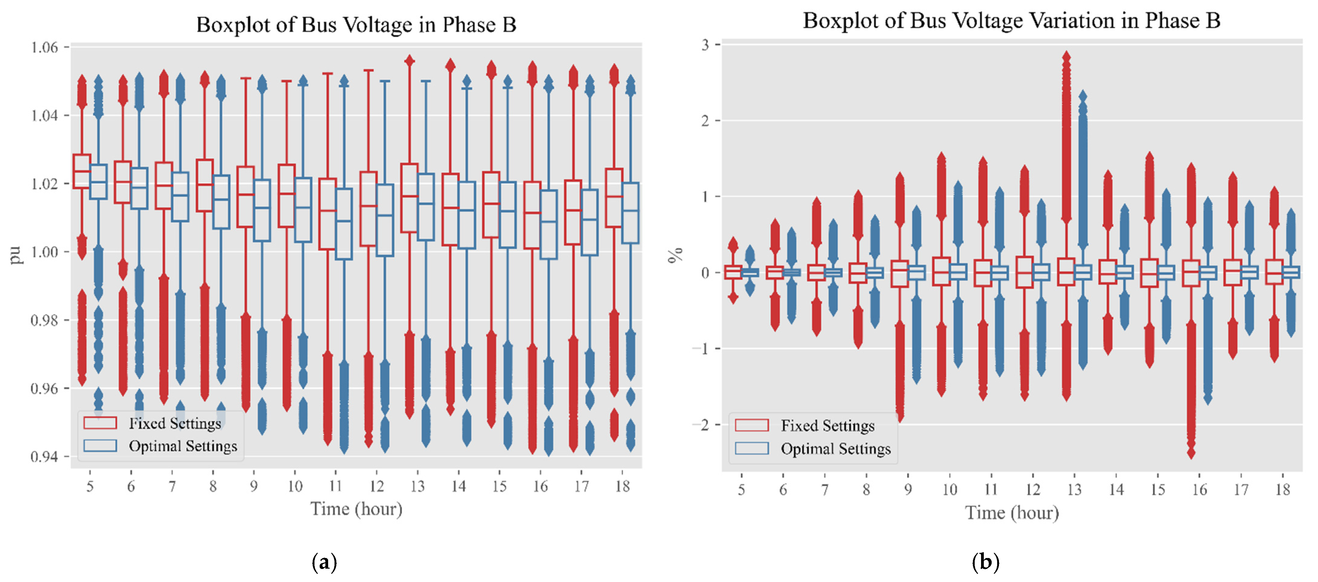
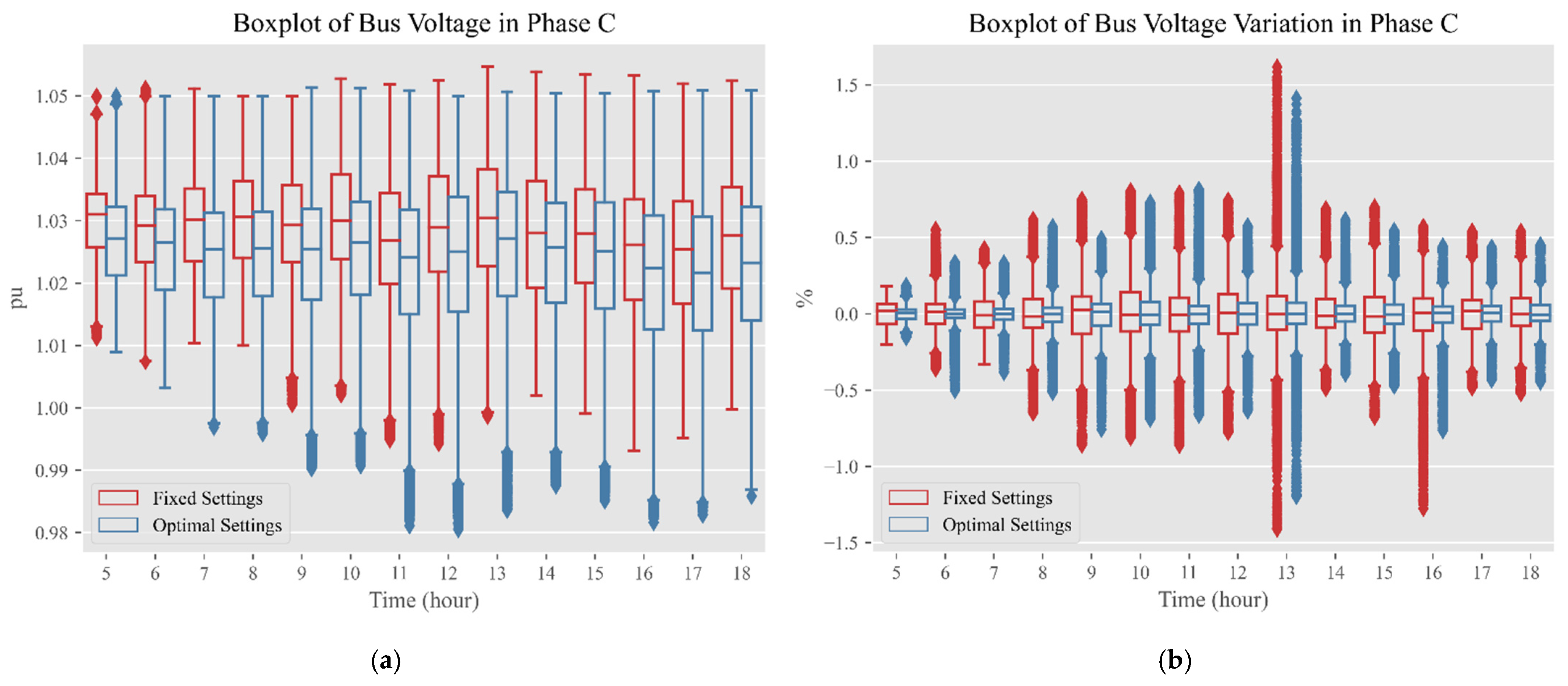
5.1. Voltage Variation

The bus voltage variation and maximum and minimum voltage deviations are optimized together to obey the grid code as expressed by $fi{t}^7$ in Equation (8). The boxplot presenting the quartiles and outlier is utilized to express the profile of individual phase bus voltage and voltage variation in each hour during all simulation periods, as shown in Figure 8, Figure 9 and Figure 10, for clarifying the distribution of the voltage data.

The original settings of all the inverters are fixed to P1(0.9, 1) and P2(1.1, −1). After optimization by the SSA, the voltage variations in the simulation period (daytime) are all clearly reduced. The maximum voltage variation is decreased from 2.83% to 2.47%; the average voltage variation is decreased from 0.20% to 0.11%. The constraint of Equation (8) is for the feeder main in the IEEE 8500-node, and the lateral bus voltage experiences undervoltage and overvoltage, as shown by the outliers in the boxplots.

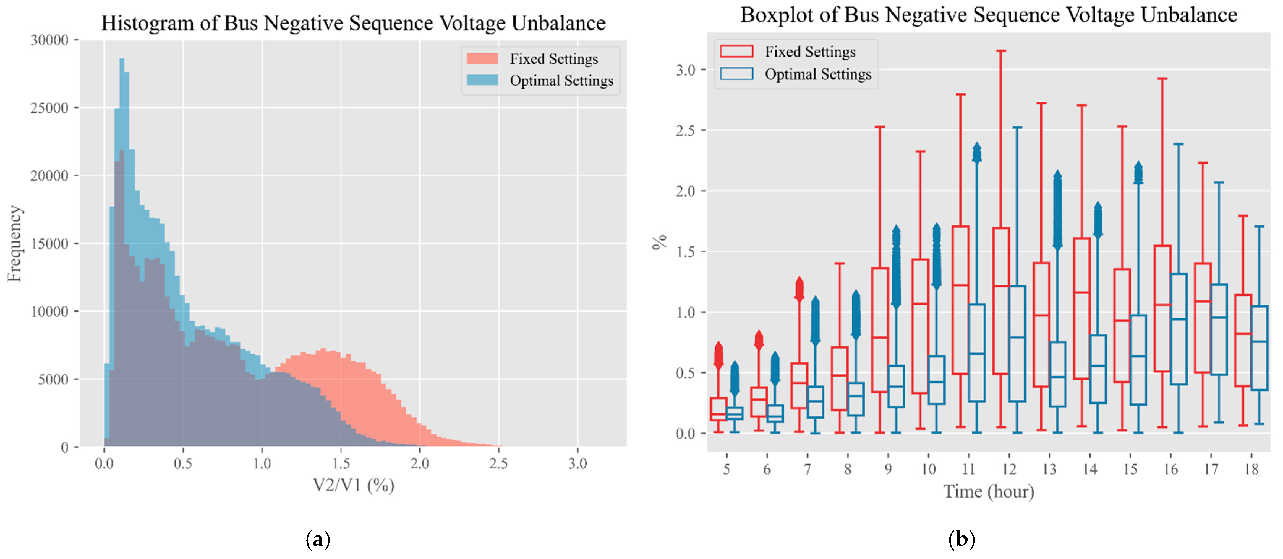
5.2. Zero and Negative Sequence Voltage Unbalance

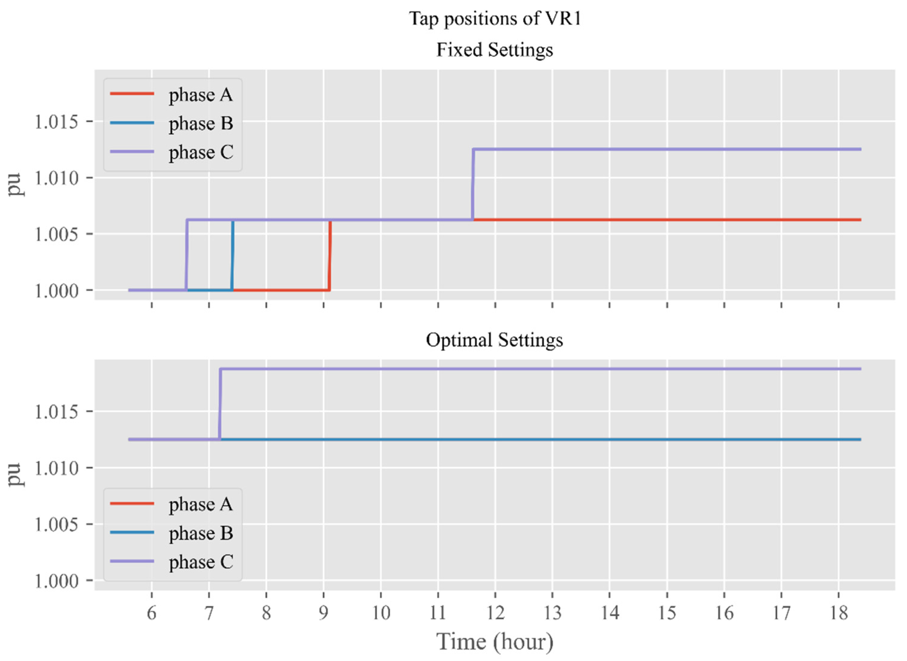
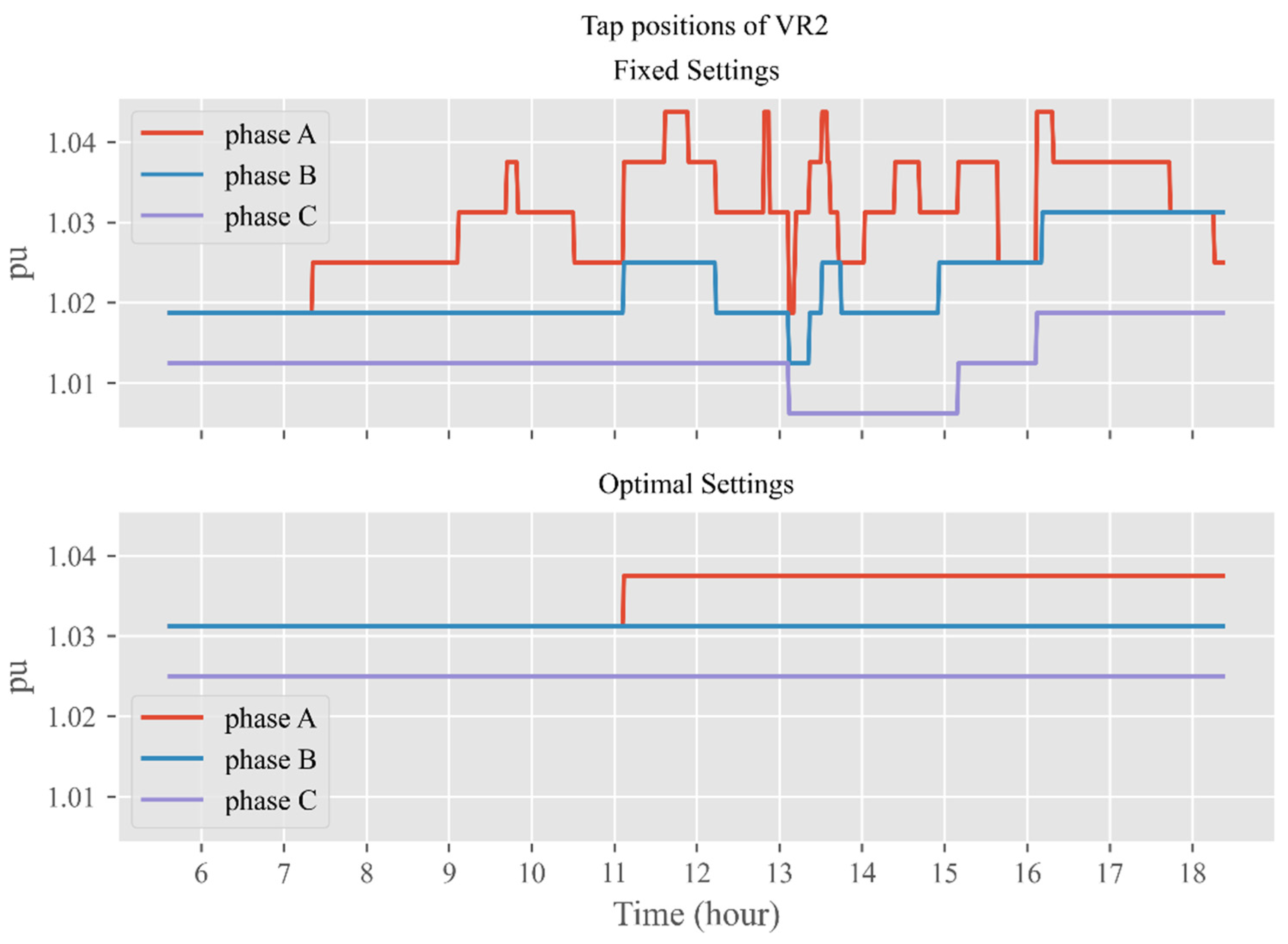
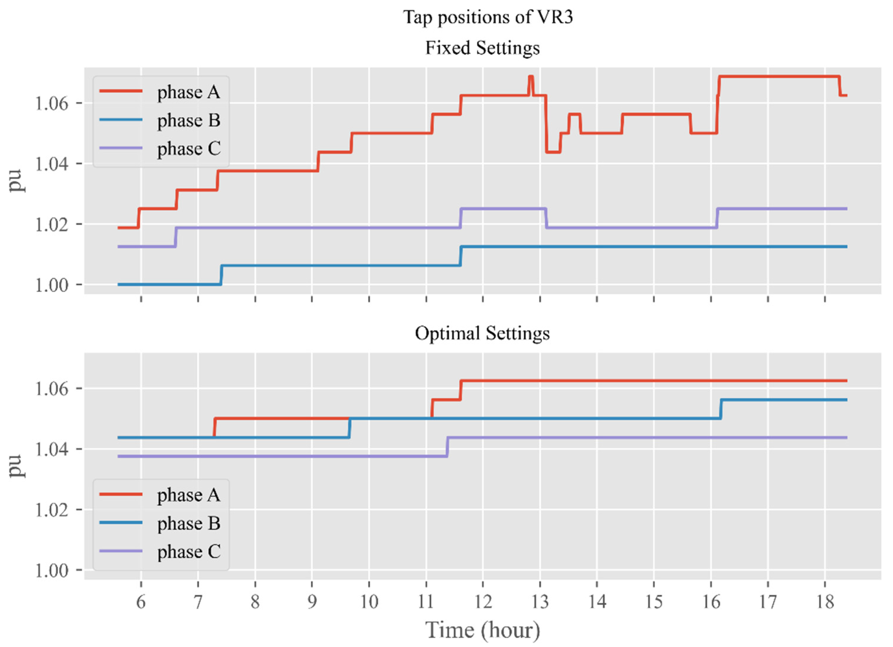
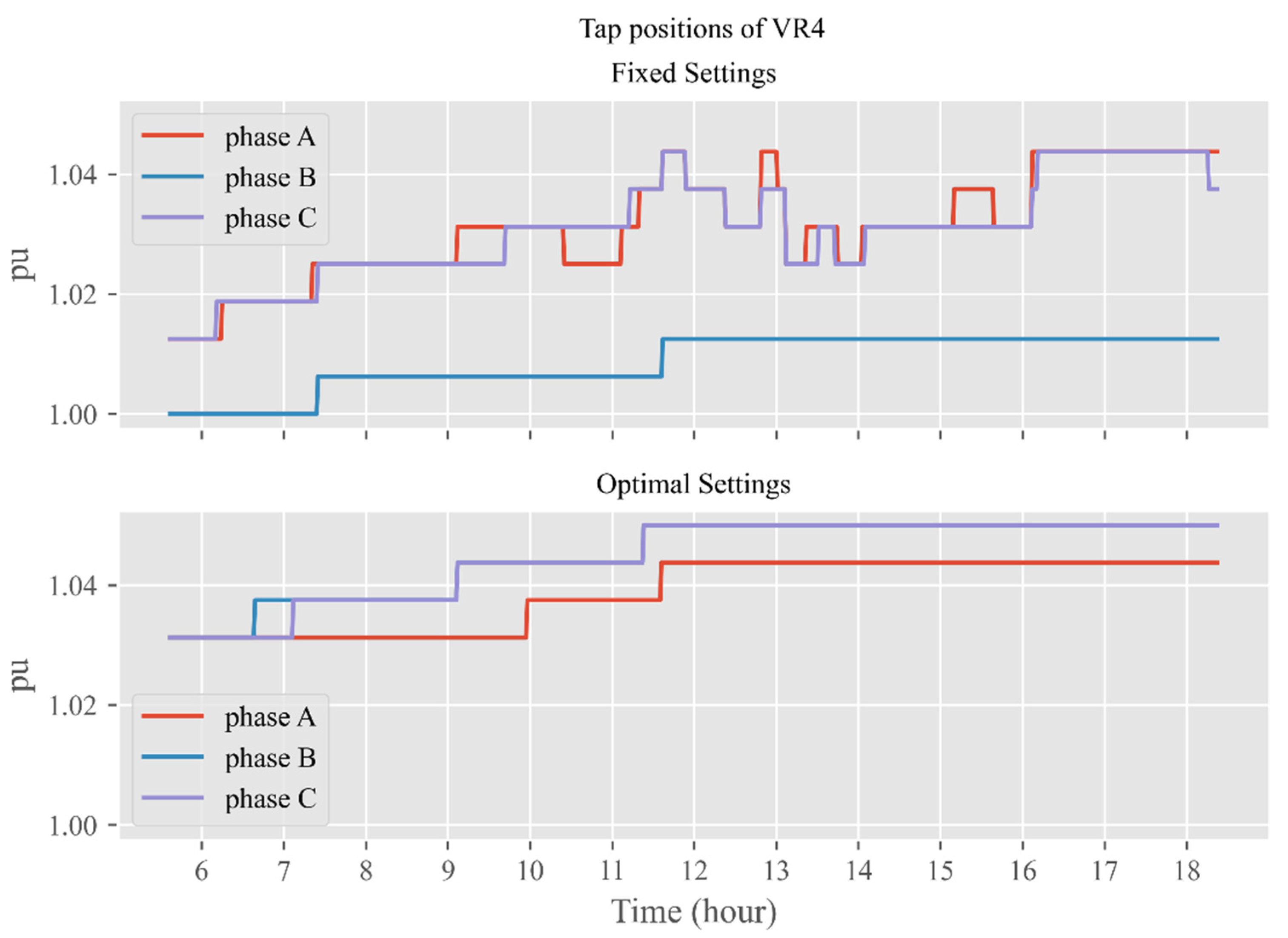
Voltage unbalances are optimized together to improve three-phase unbalance as expressed by $fi{t}^8$ in Equation (9). Figure 11 and Figure 12 show histograms that plot the distribution of the data, the zero- and negative-sequence voltage unbalances, and their boxplots in each hour during all the simulation periods.

The maximum zero-sequence voltage unbalance is decreased from 3.32% to 2.47%, and the average zero-sequence voltage unbalance is decreased from 1.08% to 0.76%. The maximum negative-sequence voltage unbalance is decreased from 3.16% to 2.52%, and the average negative-sequence voltage unbalance is decreased from 0.82% to 0.54%. The sequence voltage unbalances are significantly mitigated, and most of them are reduced to under 1.5%. The improvement near noon is also better than those in the morning and at nightfall due to the high output of the PV at noon in most patterns, as shown in Figure 6.

5.3. Tap Changing

The number of changes in VR tap positions and SCB status are optimized together for equipment deferred substitution, as expressed in Equation (7).

Table 3. The number of changes in VR tap positions and SCB status.

Equipment Name	Equipment Operation Times
	Volt–Var Control with Fixed Settings	Volt–Var Control with Optimized Settings
SCB1	0	0
SCB2	0	0
SCB3	0	0
SCB4	0	0
VR1a	1	0
VR1b	2	0
VR1c	2	1
VR2a	28	1
VR2b	8	0
VR2c	3	0
VR3a	18	3
VR3b	7	2
VR3c	4	1
VR4a	18	2
VR4b	16	3
VR4c	15	3
Total	122	16

lists the equipment operation times, and Figure 13, Figure 14, Figure 15 and Figure 16 show the three-phase tap positions of four VRs during the simulation period. The total number of changes in the VR tap positions are decreased dramatically, from 122 to 16. The SCBs are not on the grid during all of the day because the large reactive power compensation is unnecessary due to the volt–var control of the PV smart inverter.

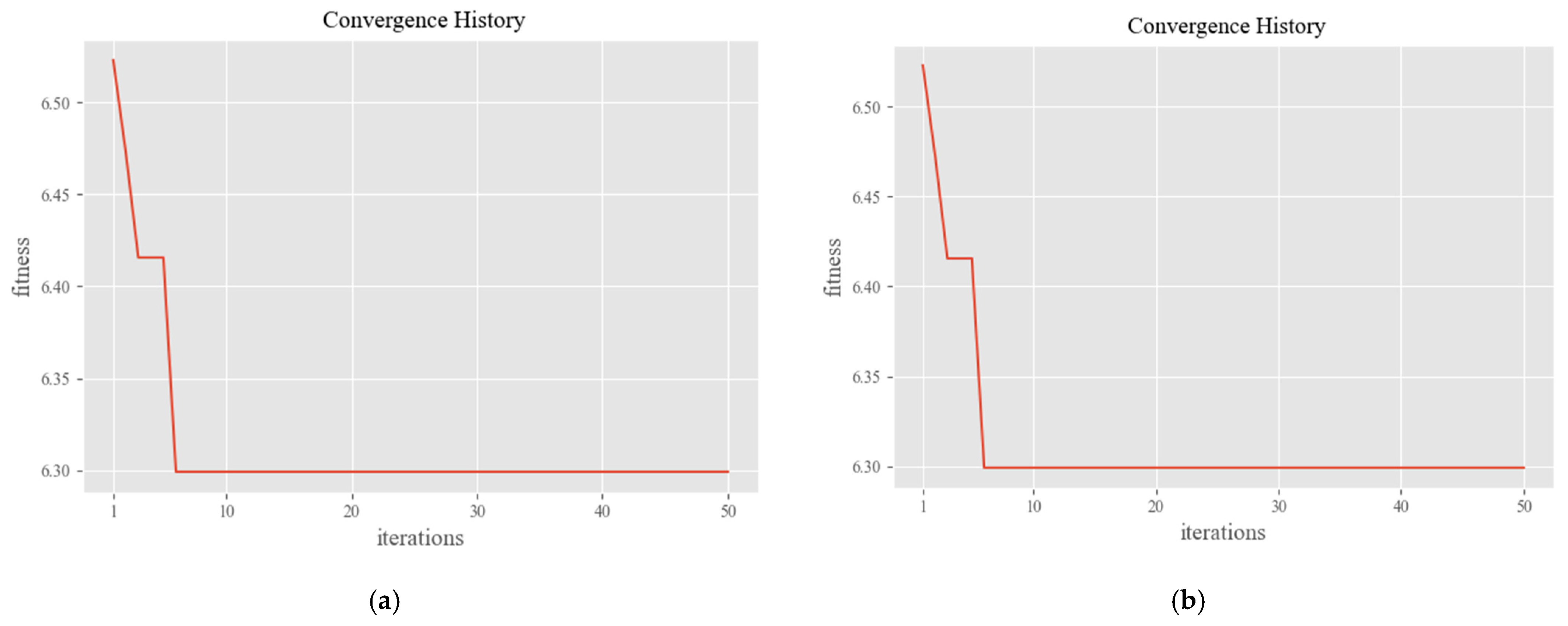
5.4. Results and Discussion

The objective functions $fi{t}^7$, $fi{t}^8$, and $fi{t}^6$ are integrated to obtain the comprehensive optimal operation in DNs. The $fi{t}^6$ function is also normalized by dividing by its best solution, $fi{t}_{best}^6$, which is 16, as solved above. Thus, the new objective function $fi{t}^9$ is expressed as Equation (16). The convergence history of the four objective functions $fi{t}^7$, $fi{t}^8$, $fi{t}^6$, and $fi{t}^9$ are shown in Figure 17. Notably, all of them converged within 50 iterations, which indicates that the SSA is a robust and stable metaheuristic algorithm for solving a complicated DN problem.

$$fi{t}^9=fi{t}^7+fi{t}^8+fi{t}^6/fi{t}_{best}^6$$

(16)

Figure 18 shows the convergence history of the top three algorithms mentioned in Table 1, which are SSA, HHO, and SO, in addition to two other popular algorithms, namely, Particle Swarm Optimization (PSO) and Grey Wolf Optimizer (GWO), for solving the objective function $fi{t}^9$. The SSA and SO have the best convergence fitness values among the five algorithms; however, the calculation time of the SSA is just half that of the SO. Therefore, the SSA has the best performance in terms of both the solution and speed.

Table 4. The optimization results of each objective function.

Objective Function	Fitness Value	Max ∆V/ Average ∆V	Max Vbus/ Min Vbus	Max V0/V1/ Average V0/V1	Max V2/V1/ Average V2/V1	N
Fixed settings	-	2.83%/ 0.20%	1.0559 pu/ 0.9402 pu	3.32%/ 1.08%	3.16%/ 0.82%	122
$fi{t}^7$ (8)	3.63	2.47%/ 0.11%	1.0519 pu/ 0.9401 pu	3.08%/ 0.94%	3.05%/ 0.82%	34
$fi{t}^8$ (9)	6.29	2.96%/ 0.14%	1.0529 pu/ 0.9402 pu	2.47%/ 0.76%	2.52%/ 0.54%	53
$fi{t}^6$ (7)	16	2.73%/ 0.11%	1.0509 pu/ 0.9325 pu	2.87%/ 0.83%	2.72%/ 0.67%	16
$fi{t}^9$ (16)	12.00	2.71%/ 0.11%	1.0529 pu/ 0.9384 pu	2.66%/ 0.83%	2.44%/ 0.67%	24

lists the results of fixed settings; objective functions $fi{t}^7$, $fi{t}^8$, $fi{t}^6$, and $fi{t}^9$; index of voltage variation ∆V; bus voltage V_bus; zero-sequence voltage unbalance V₀/V₁; negative-sequence voltage unbalance V₀/V₁; and total voltage regulation equipment operation time N. These outcomes show that each objective function can gain the best solution, but other important indices are ignored in DNs. In addition, $fi{t}^9$ can leverage between the indices well. Although the nine indices are not the best calculated by $fi{t}^9$, they are reduced simultaneously to achieve comprehensive optimization without sacrificing any other important index.

Moreover, there is little response in lateral bus voltage to changes in the control setting of the PV in the feeder main, and $fi{t}^6$ can obtain the best average ∆V due to the reduction in the number of tap position changes.

Table 5. The volt–var control settings of each PV smart inverter.

PV Information and Control Settings
Location (Bus)	Rated (kW)	V1–V2 (Pu in Phase A/B/C)	Location (Bus)	Rated (kW)	V1–V2 (Pu in Phase A/B/C)
M1125917	111	0.99–1.03/0.99–1.07/0.91–1.02	M1026780	297	0.96–1.03/0.91–1.04/0.98–1.02
M1047316	153	0.91–1.05/0.95–1.06/0.91–1.01	E183473	48	0.94–1.08/0.99–1.09/0.94–1.08
R20703	24	0.93–1.05/0.97–1.07/0.93–1.07	R42247	177	0.96–1.08/0.95–1.07/0.96–1.01
M1047737	18	0.91–1.07/0.92–1.01/0.92–1.05	L3197646	162	0.93–1.08/0.97–1.07/0.9–1.04
L2933135	222	0.99–1.04/0.99–1.06/0.96–1.02	L3207907	27	0.97–1.07/0.98–1.05/0.97–1.02
L2973167	99	0.94–1.03/0.98–1.01/0.97–1.03	N1136666	69	0.95–1.07/0.92–1.03/0.98–1.08
L3254218	195	0.94–1.06/0.94–1.07/0.91–1.04	M1026769	159	0.94–1.04/0.97–1.01/0.92–1.01
M1069509	27	0.96–1.07/0.95–1.09/0.96–1.02	N1136354	45	0.96–1.07/0.91–1.03/0.93–1.03
M1027055	27	0.94–1.08/0.91–1.02/0.97–1.09	E206217	255	0.96–1.09/0.91–1.05/0.97–1.08
M3763618	33	0.94–1.05/0.95–1.05/0.92–1.06	190–8581	84	0.98–1.08/0.92–1.07/0.94–1.05
L3048206	288	0.99–1.04/0.92–1.06/0.98–1.05	F739845	186	0.98–1.07/0.96–1.07/0.97–1.09
M1166376	30	0.93–1.05/0.92–1.01/0.96–1.04	L2766741	174	0.96–1.08/0.94–1.06/0.97–1.02
M1089196	195	0.94–1.05/0.96–1.09/0.97–1.04	N1145954	15	0.97–1.07/0.92–1.09/0.96–1.08
L3066814	294	0.98–1.07/0.95–1.06/0.95–1.03	Q16483	45	0.91–1.06/0.95–1.04/0.9–1.03
L3142049	144	0.93–1.05/0.92–1.03/0.92–1.03	M1125969	168	0.91–1.1/0.97–1.03/0.99–1.08
N1136354	99	0.93–1.06/0.96–1.07/0.96–1.04	L3181545	18	0.99–1.02/0.95–1.06/0.98–1.04
L3160107	282	0.97–1.02/0.92–1.08/0.97–1.01	N1138607	264	0.91–1.07/0.94–1.08/0.97–1.01
E206209	39	0.92–1.07/0.98–1.04/0.99–1.06	M1026670	255	0.98–1.02/0.96–1.04/0.96–1.07
M1186065	81	0.91–1.05/0.93–1.02/0.92–1.03	Q1301	276	0.97–1.07/0.94–1.06/0.98–1.04
M1026333	216	0.92–1.02/0.95–1.09/0.91–1.07	M1108500	180	0.95–1.07/0.97–1.03/0.91–1.04
M4362177	87	0.96–1.01/0.96–1.06/0.93–1.08	M1009763	228	0.99–1.03/0.93–1.04/0.92–1.04
M1047737	204	0.92–1.09/0.92–1.09/0.92–1.09	L3142049	294	0.97–1.06/0.99–1.01/0.98–1.01
M1186072	48	0.98–1.04/0.93–1.06/0.99–1.03	M1089201	54	0.92–1.02/0.93–1.02/0.95–1.09
L3081380	228	0.94–1.05/0.98–1.02/0.95–1.04	M1142828	210	0.99–1.05/0.95–1.03/0.95–1.08
L2860490	237	0.99–1.04/0.92–1.04/0.92–1.07	L3120484	63	0.93–1.03/0.95–1.03/0.94–1.07
P827527	222	0.98–1.01/0.98–1.06/0.93–1.02	L2766741	123	0.96–1.09/0.9–1.08/0.95–1.04
M1026920	291	0.99–1.05/0.94–1.09/0.92–1.01	L2691967	168	0.99–1.01/0.97–1.08/0.99–1.08
M1108535	96	0.98–1.07/0.93–1.02/0.93–1.09	M1069498	99	0.94–1.07/0.92–1.05/0.98–1.04
M1166376	114	0.93–1.02/0.99–1.05/0.93–1.09	N1138604	84	0.98–1.06/0.92–1.05/0.97–1.09
M1166374	234	0.94–1.04/0.99–1.07/0.92–1.01	L2786266	249	0.92–1.09/0.93–1.04/0.96–1.06

lists the volt–var control settings P1(V1, Q1) and P2(V2, Q2) of each PV smart inverter optimized by the objective function $fi{t}^9$.

6. Conclusions

The volt–var control settings of individual phase smart inverters distributed in DNs were optimized by the SSA in this study to obtain a voltage regulation strategy that improves the bus voltage variation, bus sequence voltage unbalance, and the voltage regulation equipment operation times. Several metaheuristics were investigated and tested, and the SSA was found to be the most appropriate for the problem investigated in this study. Furthermore, the reactive power oscillation derived from the aggressive control curve of the PV inverter was considered and constrained by the control algorithm iteration times. The maximum voltage variation on the IEEE 8500-node was reduced from 2.83% to 2.47%. Zero- and negative-sequence voltage unbalances were reduced from 3.32% to 2.47% and 3.16% to 2.52%, respectively. The number of changes in VR tap positions were reduced dramatically, from 122 to 16. The integrated objective function is also able to achieve a balance. In summary, the optimal settings of volt–var control of individual phase PVs in DNs can achieve excellent voltage control and better power quality. The outcomes of this study also provide a useful suggestion for DN operators in formulating voltage control strategies.

References

1. Renewables 2020—Analysis—IEA. Available online: https://www.iea.org/reports/renewables-2020?mode=overview (accessed on 13 November 2021).
2. Piccini, A.R.; Guimarães, G.C.; Souza, A.C.D.; Denardi, A.M. Implementation of a Photovoltaic Inverter with Modified Automatic Voltage Regulator Control Designed to Mitigate Momentary Voltage Dip. Energies 2021, 14, 6244. [Google Scholar] [CrossRef]
3. Torres, I.C.; Farias, D.M.; Aquino, A.L.L.; Tiba, C. Voltage Regulation for Residential Prosumers Using a Set of Scalable Power Storage. Energies 2021, 14, 3288. [Google Scholar] [CrossRef]
4. Almeida, D.; Pasupuleti, J.; Raveendran, S.K.; Basir Khan, M.R. Performance Evaluation of Solar PV Inverter Controls for Overvoltage Mitigation in MV Distribution Networks. Electronics 2021, 10, 1456. [Google Scholar] [CrossRef]
5. Serem, N.; Letting, L.K.; Munda, J. Voltage Profile and Sensitivity Analysis for a Grid Connected Solar, Wind and Small Hydro Hybrid System. Energies 2021, 14, 3555. [Google Scholar] [CrossRef]
6. Nakadomari, A.; Shigenobu, R.; Kato, T.; Krishnan, N.; Hemeida, A.M.; Takahashi, H.; Senjyu, T. Unbalanced Voltage Compensation with Optimal Voltage Controlled Regulators and Load Ratio Control Transformer. Energies 2021, 14, 2997. [Google Scholar] [CrossRef]
7. Yuvaraj, T.; Devabalaji, K.R.; Prabaharan, N.; Haes Alhelou, H.; Manju, A.; Pal, P.; Siano, P. Optimal Integration of Capacitor and Distributed Generation in Distribution System Considering Load Variation Using Bat Optimization Algorithm. Energies 2021, 14, 3548. [Google Scholar] [CrossRef]
8. Montoya, O.D.; Molina-Cabrera, A.; Grisales-Noreña, L.F.; Hincapié, R.A.; Granada, M. Improved Genetic Algorithm for Phase-Balancing in Three-Phase Distribution Networks: A Master-Slave Optimization Approach. Computation 2021, 9, 67. [Google Scholar] [CrossRef]
9. Danish, S.M.S.; Shigenobu, R.; Kinjo, M.; Mandal, P.; Krishna, N.; Hemeida, A.M.; Senjyu, T. A Real Distribution Network Voltage Regulation Incorporating Auto-Tap-Changer Pole Transformer Multiobjective Optimization. Appl. Sci. 2019, 9, 2813. [Google Scholar] [CrossRef] [Green Version]
10. Su, X.; Liu, J.; Tian, S.; Ling, P.; Fu, Y.; Wei, S.; SiMa, C. A Multi-Stage Coordinated Volt-Var Optimization for Integrated and Unbalanced Radial Distribution Networks. Energies 2020, 13, 4877. [Google Scholar] [CrossRef]
11. Alzahrani, A.; Alharthi, H.; Khalid, M. Minimization of Power Losses through Optimal Battery Placement in a Distributed Network with High Penetration of Photovoltaics. Energies 2020, 13, 140. [Google Scholar] [CrossRef] [Green Version]
12. Lee, Y.-D.; Jiang, J.-L.; Ho, Y.-H.; Lin, W.-C.; Chih, H.-C.; Huang, W.-T. Neutral Current Reduction in Three-Phase Four-Wire Distribution Feeders by Optimal Phase Arrangement Based on a Full-Scale Net Load Model Derived from the FTU Data. Energies 2020, 13, 1844. [Google Scholar] [CrossRef]
13. Zeraati, M.; Golshan, M.E.H.; Guerrero, J.M. A Consensus-Based Cooperative Control of PEV Battery and PV Active Power Curtailment for Voltage Regulation in Distribution Networks. IEEE Trans. Smart Grid 2019, 10, 670–680. [Google Scholar] [CrossRef] [Green Version]
14. Oh, C.-H.; Choi, J.-H.; Yun, S.-Y.; Ahn, S.-J. Short-Term Cooperative Operational Scheme of Distribution System with High Hosting Capacity of Renewable-Energy-Based Distributed Generations. Energies 2021, 14, 6340. [Google Scholar] [CrossRef]
15. Xiao, H.; Pei, W.; Dong, Z.; Kong, L.; Wang, D. Application and Comparison of Metaheuristic and New Metamodel Based Global Optimization Methods to the Optimal Operation of Active Distribution Networks. Energies 2018, 11, 85. [Google Scholar] [CrossRef] [Green Version]
16. Alyami, S.; Wang, Y.; Wang, C.; Zhao, J.; Zhao, B. Adaptive Real Power Capping Method for Fair Overvoltage Regulation of Distribution Networks With High Penetration of PV Systems. IEEE Trans. Smart Grid 2014, 5, 2729–2738. [Google Scholar] [CrossRef]
17. Ammar, M.; Sharaf, A.M. Optimized Use of PV Distributed Generation in Voltage Regulation: A Probabilistic Formulation. IEEE Trans. Ind. Inform. 2019, 15, 247–256. [Google Scholar] [CrossRef]
18. Chamana, M.; Chowdhury, B.H. Optimal Voltage Regulation of Distribution Networks with Cascaded Voltage Regulators in the Presence of High PV Penetration. IEEE Trans. Sustain. Energy 2018, 9, 1427–1436. [Google Scholar] [CrossRef]
19. Gerdroodbari, Y.Z.; Razzaghi, R.; Shahnia, F. Improving Voltage Regulation and Unbalance in Distribution Networks using Peer-to-Peer Data Sharing between Single-phase PV Inverters. IEEE Trans. Power Deliv. 2021. [Google Scholar] [CrossRef]
20. Wang, L.; Bai, F.; Yan, R.; Saha, T.K. Real-Time Coordinated Voltage Control of PV Inverters and Energy Storage for Weak Networks with High PV Penetration. IEEE Trans. Power Syst. 2018, 33, 3383–3395. [Google Scholar] [CrossRef] [Green Version]
21. Zhang, Y.; Srivastava, A. Voltage Control Strategy for Energy Storage System in Sustainable Distribution System Operation. Energies 2021, 14, 832. [Google Scholar] [CrossRef]
22. Xu, T.; Meng, H.; Zhu, J.; Wei, W.; Zhao, H.; Yang, H.; Li, Z.; Wu, Y. Optimal Capacity Allocation of Energy Storage in Distribution Networks Considering Active/Reactive Coordination. Energies 2021, 14, 1611. [Google Scholar] [CrossRef]
23. Wang, J.; Kang, L.; Liu, Y. Optimal design of a cooperated energy storage system to balance intermittent renewable energy and fluctuating demands of hydrogen and oxygen in refineries. Comput. Chem. Eng. 2021, 155, 107543. [Google Scholar] [CrossRef]
24. Saini, P.; Gidwani, L. An investigation for battery energy storage system installation with renewable energy resources in distribution system by considering residential, commercial and industrial load models. J. Energy Storage 2021, 103493. [Google Scholar] [CrossRef]
25. Waswa, L.; Chihota, M.J.; Bekker, B. A Probabilistic Conductor Size Selection Framework for Active Distribution Networks. Energies 2021, 14, 6387. [Google Scholar] [CrossRef]
26. Liu, Y.-J.; Tai, Y.-H.; Lee, Y.-D.; Jiang, J.-L.; Lin, C.-W. Assessment of PV Hosting Capacity in a Small Distribution System by an Improved Stochastic Analysis Method. Energies 2020, 13, 5942. [Google Scholar] [CrossRef]
27. Čađenović, R.; Jakus, D. Maximization of Distribution Network Hosting Capacity through Optimal Grid Reconfiguration and Distributed Generation Capacity Allocation/Control. Energies 2020, 13, 5315. [Google Scholar] [CrossRef]
28. Schoene, J.; Zheglov, V.; Humayun, M.; Poudel, B.; Kamel, M.; Gebeyehu, A.; Garcia, M.; Robles, S.; Son, H. Investigation of oscillations caused by voltage control from smart PV on a secondary system. In Proceedings of the 2017 IEEE Power & Energy Society General Meeting, Chicago, IL, USA, 16–20 July 2017; pp. 1–5. [Google Scholar] [CrossRef]
29. Xue, J.; Shen, B. A novel swarm intelligence optimization approach: Sparrow search algorithm. Syst. Sci. Control Eng. 2020, 8, 22–34. [Google Scholar] [CrossRef]
Figure 1. Capability curves of: (a) PV inverter; (b) BESS inverters.
Energies 14 08370 g001
Figure 2. Voltage, and active and reactive power, of the PV smart inverter with volt–var control.
Energies 14 08370 g002
Figure 3. Volt-var control curve setting.
Energies 14 08370 g003
Figure 4. Oscillation of V and Q caused by different volt-var control settings.
Energies 14 08370 g004
Figure 5. Sample system.
Energies 14 08370 g005
Figure 6. PV output patterns.
Energies 14 08370 g006
Figure 7. Flow chart of the optimization solution framework.
Energies 14 08370 g007
Figure 8. Boxplots of (a) bus voltage and (b) voltage variation in phase A for each hour with fixed and optimal volt-var control settings.
Energies 14 08370 g008
Figure 9. Boxplots of (a) bus voltage and (b) voltage variation in phase B for each hour with fixed and optimal volt-var control settings.
Energies 14 08370 g009
Figure 10. Boxplots of (a) bus voltage and (b) voltage variation in phase C for each hour with fixed and optimal volt–var control settings.
Energies 14 08370 g010
Figure 11. Zero sequence voltage unbalance: (a) Histogram; (b) Boxplot.
Energies 14 08370 g011
Figure 12. Negative sequence voltage unbalance: (a) Histogram; (b) Boxplot in each hour.
Energies 14 08370 g012
Figure 13. Three-phase tap positions of VR1.
Energies 14 08370 g013
Figure 14. Three-phase tap positions of VR2.
Energies 14 08370 g014
Figure 15. Three-phase tap positions of VR3.
Energies 14 08370 g015
Figure 16. Three-phase tap positions of VR4.
Energies 14 08370 g016
Figure 17. The convergence history of the SSA for the four objective functions. (a) Objective function fit7 (for voltage variation), (b) Objective function fit8 (for sequence voltage unbalance), (c) Objective function fit6 (for number of changes in tap position), (d) Objective function fit9 (for comprehensive optimization).
Energies 14 08370 g017aEnergies 14 08370 g017b
Figure 18. The convergence history comparison of the SSA and other metaheuristics for f i t 9 .
Energies 14 08370 g018