Optimal Location and Sizing of Renewable Distributed Generators for Improving Voltage Stability and Security Considering Reactive Power Compensation

Abstract

The integration of renewable resources into the existing power distribution system is expanding to reduce gas emissions, treat climate change and satisfy the current global need for clean energy. If the location and size of these renewable generators are determined without considering uncontrollable reactive power compensation caused by their intermittent nature, the resultant power system may suffer from system instability and decreased reliability. Therefore, the issue of optimal location and size of renewable resources attracts great attention. In this paper, a methodology is proposed to optimize the locations and capacities of distributed renewable generators installed in conventional power distribution systems. In particular, uncontrollable reactive power compensation of these renewable resources is considered in this paper and managed through the proposed methodology to ensure power system reliability and stability. As a result, the proposed methodology reminds us of the importance of reactive power compensation by performing better in power losses reduction and the robustness of voltage stability against variable reactive power compensation.

1. Introduction

By considering the depletion of conventional power sources, growing energy demand, the necessity to reduce gas emissions etc., renewable distributed generators (RDGs) have been promoted worldwide [1,2,3]. These energy generators are environmentally friendly and can be used as alternatives to conventional dispatchable generators. The defining characteristics of non-dispatchable RDGs (e.g., Photovoltaic (PV) and Wind Turbine (WT)) are unsteady and non-uniform compared with the conventional dispatchable sources, such as oil, natural gas and coal. Due to their intermittent nature, hybrid mixtures of two or more power generation systems can enhance the power quality, improve system reliability, reduce power losses and increase the efficiency of the power system [4,5]. However, the inappropriate placement of RDGs leads to increasing power losses, and degradation of voltage stability [6,7,8,9].

Optimal location and size of RDGs have attracted numerous studies in recent years. Many researchers have focused on developing methodologies for determining the optimal location and size for minimizing power losses [10,11,12,13,14,15,16,17,18,19] and improving voltage profile [11,13,17]. The authors of [11] developed the Evolution Programming (EP) method which incorporates the correlation between loads and renewable sources and allows the wind power to be dispatched to a certain fraction of system load. The authors of [12] applied the Ant Lion Optimization Algorithm (ALOA) to determine the optimal placement of RDGs resulting in a minimum power transmission loss. The authors of [13] applied the Whale Optimization Algorithm (WOA) to determine the optimal location and size of RDGs resulting in a minimum power loss and improved voltage profile in terms of Voltage Sensitivity Index (VSI). The authors of [14] proposed the methodology to determine the size of RDGs considering the time-varying characteristics of both generators and loads. The authors of [15] used Particle Swarm Optimization (PSO) to determine the optimal location and size considering the minimization of Total Harmonic Distortion (THD) and uncertainty of loads and future growth of them. The authors of [16] developed the meta-heuristic method for determining the placement of RDGs, which can converge to an optimal solution even for a non-convex problem. The authors of [17] developed the Improved Gravitational Search Algorithm (IGSA) to determine the optimal location and size of RDGs considering the THD. The authors of [18] modified the PSO and Gravitational Search Algorithm (GSA) to determine sizes and locations of DGs and shunt capacitors resulting in better solutions in terms of power losses and THD reduction. The authors of [19] proposed the algorithm for detecting the vulnerable buses using VSI, and determined the optimal location and size of RDGs using Multi Leader Particle Swarm Optimization (MLPSO). Recently, the authors of [20] proposed the improved meta-heuristic method, called the b-chaotic sequence spotted hyena optimizer, for determining the optimal size and location of wind turbines considering reducing power losses and improving voltage profile. This method reached the minimum power losses and improved the voltage profiles. The authors of [21] proposed a hybrid technique, called the tunicate swarm algorithm/sine-cosine algorithm (TSA/SCA), for determining the optimal allocation of RDGs in different scenarios considering power losses. Most of the studies presented above did not consider reactive power compensation of generators, which affects voltage stability and security from voltage collapse.

Since reactances dominate power distribution networks in voltage control [22], voltage instability is affected not only by uncontrollable loads and generators but also by reactive power compensation of renewable distributed generators (RDGs). Therefore, uncontrollable reactive power consumption is needed to be investigated for the optimal placement determination. By considering the capacity of reactive support, which is the ability of the system to support reactive power compensation, a methodology of the optimal location and size determination is proposed. At first, several key functions such as the voltage product (v-p) function, the active v-p function, and the reactive v-p function, are derived from the fundamental complex power formula, which are used for calculating voltage stability in each bus. For estimating the most vulnerable bus of voltage collapse, a safety margin, Reactive Power Compensation Support Margin for Voltage Stability Improvement (QSVS) is then formulated with these key functions.

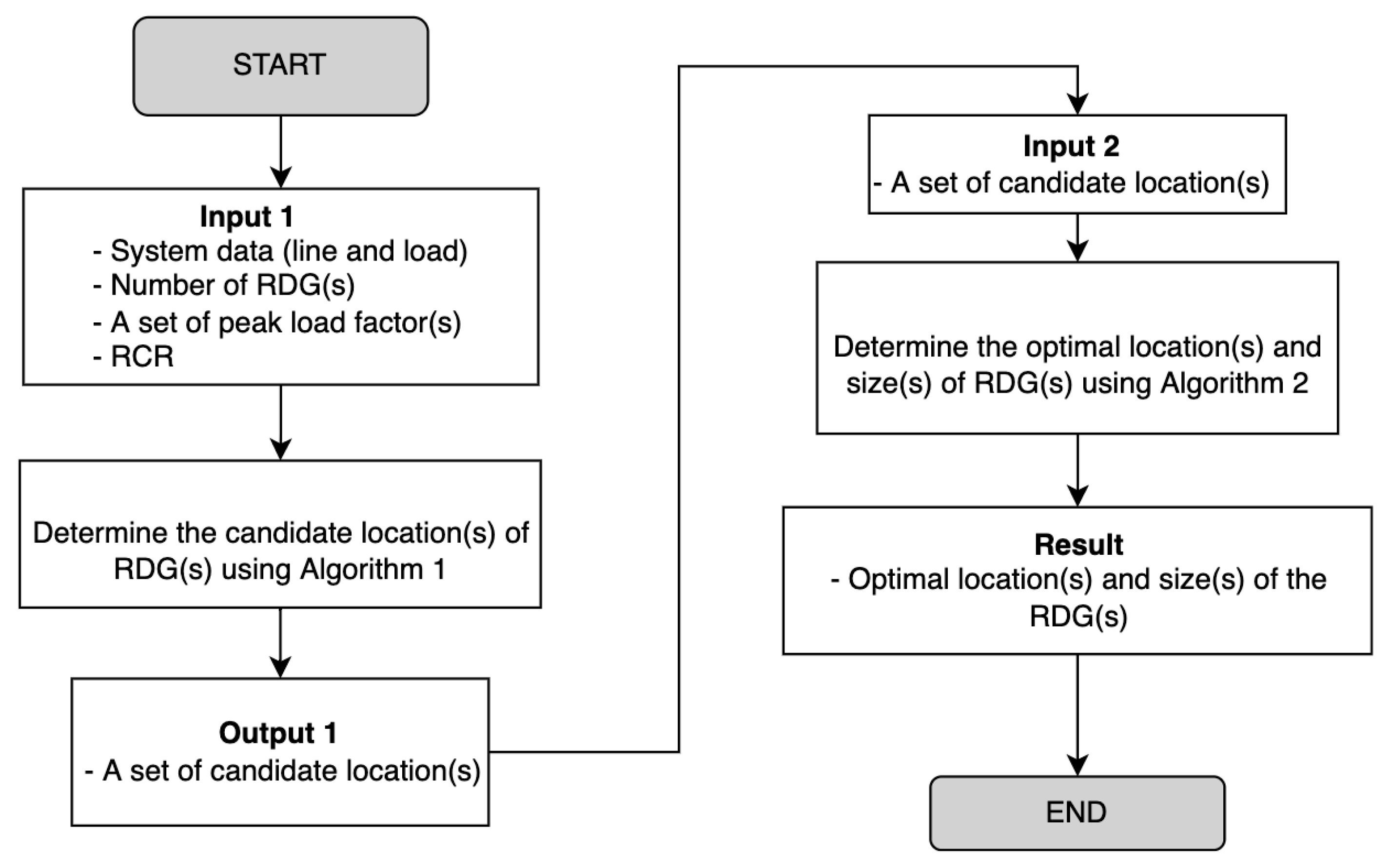
The proposed methodology for determining the placement of RDGs is divided into two parts. The first part is the determination of an optimal location using the proposed QSVS as the objective function to be maximized, and the second part is the determination of an optimal size for minimizing system power loss of power systems. By considering the reactive compensation and the safety margin using QSVS in the optimal location and size determination, the proposed methodology gives us better results in terms of power losses reduction and voltage stability improvement.

The rest of the paper is organized as follows. Section 2 describes the preliminary study with system models, voltage stability index, and the formulation of power losses calculations. Section 3 describes the basic idea of voltage stability assessment, related mathematical key functions, the formulation of QSVS, the reactive compensation effect, and the proposed mathematical function for the optimal design with QSVS. Then, Section 4 introduces a methodology including algorithms of the optimal location and sizing of RDGs. In Section 5, simulations and discussions are described. Finally, Section 6 presents the concluding remarks.

2. Preliminary

2.1. System Model

Basically, power flows from the slack bus to loads connected to the bus through power lines in a power distribution system. The information concerning power consumption levels, single line diagram, and line impedance is given in the form of an IEEE test distribution system. The information of the maximum levels of power consumption of loads are necessary when maximum power losses and voltage stability are investigated. In this paper, both maximum power generation and power consumption are only considered in a steady state.

The following assumptions are made to develop the mathematical model for optimal placement of RDGs in a power distribution system:

• The number of RDGs to be installed is given.
• Since the generated active power is uncontrollable in a steady-state, in order to maintain the voltage at the nominal level, reactive compensation of RDGs is assumed to be consumed depending on their generated active power multiplied by reactive power compensation ratio (RCR). Therefore, the effect of uncontrollable reactive compensation of RDGs associated with their generated power is evaluated using RCR.
• The impacts of unbalanced load and compensation of both active and reactive power are neglected.

2.2. Voltage Stability Index

For determining the optimal location of RDGs, the voltage stability limit dominated by generator reactive consumption is our primary concern. The L-index proposed by [23], which delineates quantitative measurement of a weak bus and forecasting of voltage collapse, is used as one of the measures to evaluate a system. The L index is formulated as shown in Equation (1):

$$L=\underset{j\in \mathcal{T}}{\max }\left|1-\frac{{\sum }_{i\in \mathcal{S}}{\overline{F}}_{ji}{\overline{V}}_i}{{\overline{V}}_j}\right|$$

(1)

where

${\overline{V}}_i$,${\overline{V}}_j$—complex voltages of the ith and jth buses, respectively,

$\mathcal{T}$—a set of loads,

$\mathcal{S}$—a set of generators,

${\overline{F}}_{ji}$—the jth row, ith column element of the hybrid matrix, which is generated from the matrix Y by a partial inversion, described in [23].

Under stable operation, the value of the L-index should be less than 1, and the smaller the value of the L-index from 1, the more stable the system.

2.3. Total Power Losses

Due to electrical resistance in power lines, power losses occur. Several studies demonstrated that the location and size of distributed generators (DGs) play an essential role in the reduction of total power losses. The power losses can be expressed as Equation (2) [24].

$$P_{loss}=\sum _{m=1}^N\sum _{n=1}^N\left(a_{mn}(P_m{P}_n+Q_m{Q}_n)+b_{mn}(Q_m{P}_n-P_m{Q}_n)\right)$$

(2)

where

$$a_{mn}=\frac{r_{mn}}{V_m{V}_n}cos({\delta }_m-{\delta }_n),$$

$$b_{mn}=\frac{r_{mn}}{V_m{V}_n}sin({\delta }_m-{\delta }_n),$$

$V_m$,$V_n$—voltage magnitudes of the mth and nth buses, respectively,

${\delta }_m$,${\delta }_n$—voltage angles of the mth and nth buses, respectively,

$r_{mn},x_{mn}$—resistance and reactance of the mth row, nth column element of the impedance matrix $Z_{bus}$,

$P_m$,$P_n$—active power injections at the mth and nth buses, respectively,

$Q_m$, $Q_n$—reactive power injections at the mth and nth buses, respectively,

N—the number of buses.

2.4. Loading Margin

The loading margin, a fundamental measure of closeness to voltage collapse [25], is used to estimate the limitation of the increment of load. In this paper, the loading margin is also used to evaluate a system in the proximity to voltage collapse blackouts. Furthermore, to guarantee safety from voltage collapse, the minimum loading margin is demonstrated for every optimal RDG placement.

3. Voltage Stability and Security

To support the installation of renewable energy sources and their uncontrollable reactive power compensation, the enhancement of voltage stability and security from voltage collapse are considered. In the following section, first, the basic idea of voltage stability assessment is described. Then, mathematical functions are introduced for describing system characteristics. Next, voltage collapse caused by the reactive compensation is investigated. Finally, a mathematical function of voltage stability and security is formulated, which can be used as the objective function for the optimal placement of RDGs.

3.1. Basic Idea of Voltage Stability Assessment

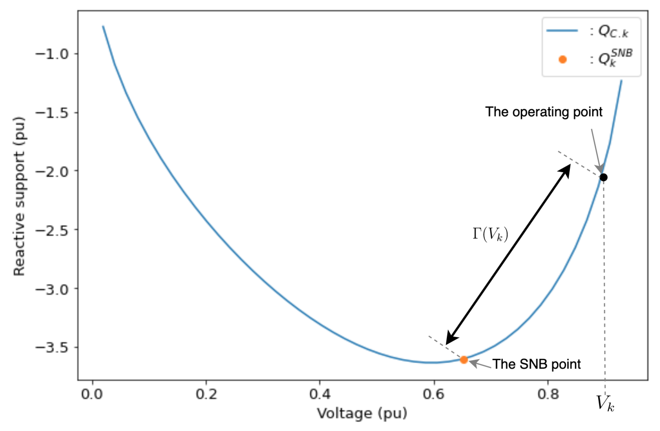
Voltage stability is defined as the ability to maintain the voltage level of each bus in an acceptable range during normal operation as well as after any contingency events [26]. The voltage stability can be described by the relationship between reactive support ($Q_c$) at a given bus and the voltage at that bus using the VQ curve. The positive value of $Q_c$ means the system requires external reactive power injection to system operability. The negative value of $Q_c$ indicates that the system sufficiently provides reactive power margins for compensations of an operating point. Figure 1 shows an example of reactive support in the VQ curve of the kth bus on a test distribution system. Under stable operation, the summation of $Q_c$ and external reactive power must be equal to zero. Therefore, one factor controlling the voltage stability is the value of $Q_c$. Therefore, one factor controlling the voltage stability is the value of $Q_c$.

In the VQ curve, the critical point, known as the saddle nodal bifurcation (SNB), is the loading point at the voltage collapse [26,27]. The operating point must be kept away from the voltage collapse. Since voltage collapse, which is a system instability, can be caused by uncontrollable reactive power compensation of RDG. Therefore, the voltage stability assessment function considering the voltage collapse needs to be made for the determination of optimal placement of RDGs.

To maintain voltage stability, not only must the reactive power $Q_c$ sufficiently provide reactive power margins for compensation of an operating point, but the distance between the SNB point and operating point must be increased for preventing voltage collapses.

3.2. Mathematical Formulations

3.2.1. Mathematical Key Functions

To develop the fundamental complex power equation, ${\overline{S}}^{*}={\overline{V}}^{*}\overline{I}$, into non-complex functions form, the mathematical key functions are introduced, which is to be used for forming the voltage stability indicator.

For any kth bus,

$$\begin{array}{cc}\hfill {\overline{S}}_k^{*}& ={\overline{V}}_k^{*}{\overline{I}}_k\hfill \\ \hfill {\overline{S}}_k^{*}& ={\overline{V}}_k^{*}\sum _{n=1}^N{\overline{Y}}_{nk}{\overline{V}}_n\hfill \end{array}$$

which can be converted to

$$\begin{array}{cc}\hfill \frac{{\overline{S}}_k^{*}}{{\overline{Y}}_{kk}}& =(\frac{{\sum }_{n=1,\ne k}^N{\overline{Y}}_{nk}{\overline{V}}_n}{{\overline{Y}}_{kk}}){\overline{V}}_k^{*}+V_k^2\hfill \end{array}$$

(3)

The voltage product (v-p) function (${\overline{\psi }}_k$) at the kth bus is defined as

$$\begin{array}{cc}\hfill & {\overline{\psi }}_k\stackrel{▵}{=}\frac{{\sum }_{n=1,n\ne k}^N{\overline{Y}}_{nk}{\overline{V}}_n}{{\overline{Y}}_{kk}}\hfill \end{array}$$

(4)

where

${\overline{V}}_n$

 the complex voltage at the nth bus,

${\overline{Y}}_{mn}$

 the mth row, the nth column complex element of the admittance matrix ${\mathrm{Y}}_{bus}$,

N 

 the number of buses.

Then, by substitution of ${\overline{\psi }}_k$, Equation (3) can be rewritten as;

$$\begin{array}{cc}\hfill \frac{{\overline{S}}_k^{*}}{{\overline{Y}}_{kk}}& ={\overline{\psi }}_k{\overline{V}}_k^{*}+V_k^2\hfill \end{array}$$

(5)

Likewise, Equation (5) takes the form

$$\begin{array}{c}\hfill {\overline{\psi }}_k{\overline{V}}_k^{*}+V_k^2={\psi }_k{V}_{k}cos({\zeta }_k-{\delta }_k)+j{\psi }_k{V}_{k}sin({\zeta }_k-{\delta }_k)+V_k^2\end{array}$$

(6)

where ${\psi }_k$ and ${\zeta }_k$ are the v-p magnitude, the v-p angle of the kth bus, respectively.

Separating Equation (6) into real and imaginary parts, we have

$$\begin{array}{cc}\hfill {\psi }_{P.k}(V_k,{\Delta }_k)& \stackrel{▵}{=}{V}_k^2+{\psi }_k{V}_{k}cos\left({\Delta }_k\right)\hfill \end{array}$$

(7)

$$\begin{array}{cc}\hfill {\psi }_{Q.k}(V_k,{\Delta }_k)& \stackrel{▵}{=}{\psi }_k{V}_{k}sin\left({\Delta }_k\right)\hfill \end{array}$$

(8)

where ${\Delta }_k={\zeta }_k-{\delta }_k$. For simplification, ${\psi }_{P.k}$ and ${\psi }_{Q.k}$ are used for ${\psi }_{P.k}(V_k,{\Delta }_k)$ and ${\psi }_{Q.k}(V_k,{\Delta }_k)$ if the augments are clear from the context. In the following, ${\psi }_{P.k}$ and ${\psi }_{Q.k}$ are called active v-p function and reactive v-p function, respectively.

For calculating the magnitude of the voltage at the kth bus using ${\psi }_{Q.k}$ and ${\psi }_k$, first we substitute Equations (7) and (8) into Equation (6) to obtain the bus voltage equation as

$$V_k^4-V_k^2\left({\psi }_k^2+2{\psi }_{P.k}\right)+{\psi }_{P.k}^2+{\psi }_{Q.k}^2=0$$

(9)

3.2.2. Reactive Support Q_c

Voltage solutions which are obtained from Equation (9) are the feasible power flow solution. Once the solution is investigated using the VQ curve, the reactive support $Q_C$ is obtained from Equation (9) as

$$\begin{array}{cc}\hfill Q_{C.k}& =-\frac{Y_{kk}sin\left({\varphi }_k\right)}{sin({\varphi }_k+{\theta }_{kk})}·{\psi }_{Q.k}\hfill \end{array}$$

(10)

where ${\psi }_{Q.k}$ is obtained from Equation (8), and

$Q_k$—the magnitude of reactive power injection at the kth bus,

$Q_{C.k}$—the magnitude of reactive support at the kth bus,

${\varphi }_k$—the angle of the phasor of complex power injection ${\overline{S}}_k$ at the kth bus,

$Y_{kk}$—the magnitude of the kth row, the kth column complex element of the admittance matrix ${\mathrm{Y}}_{bus}$,

${\theta }_{kk}$—the angle of the kth row, the kth column complex element of the admittance matrix ${\mathrm{Y}}_{bus}$.

Please note that the negative solution of $Q_{C.k}$ means stable in voltage without requiring external reactive power injection and the positive solution of $Q_{C.k}$ means stable in voltage with requiring external reactive power injection to maintain the voltage level within an acceptable range. Therefore, $Q_c$ is the key to indicating the ability of voltage stability.

3.2.3. Identification of Voltage Collapse

As the discussion in [22,23,28], the power flow Jacobian matrix becomes singular at the point of voltage collapse or the saddle node bifurcation (SNB).

From Equations (7) and (8), the singularity of Jacobian matrix can be written as

$$\begin{array}{c}\hfill \left|\begin{array}{cc}\frac{\partial {\psi }_{P.k}}{\partial V_k}& \frac{\partial {\psi }_{P.k}}{\partial {\Delta }_k}\\ \frac{\partial {\psi }_{Q.k}}{\partial V_k}& \frac{\partial {\psi }_{Q.k}}{\partial {\Delta }_k}\end{array}\right|=0\end{array}$$

$$\begin{array}{c}\hfill \left|\begin{array}{cc}2V_k+{\psi }_{k}cos\left({\Delta }_k\right)& -V_k{\psi }_{k}sin\left({\Delta }_k\right)\\ {\psi }_{k}sin\left({\Delta }_k\right)& V_k{\psi }_{k}cos\left({\Delta }_k\right)\end{array}\right|=0\end{array}$$

$$\begin{array}{c}\hfill V_k{\psi }_k\left(2V_{k}cos\left({\Delta }_k\right)+{\psi }_k\right)=0\end{array}$$

(11)

The SNB condition using Equation (11) can be written as

$${\psi }_k=-2V_{k}cos\left({\Delta }_k\right)$$

(12)

By considering the feasible solution of the voltage from Equation (9) with substituting Equations (7) and (8) and the SNB condition of Equation (12), the voltage $V_k^{SNB}$ at the SNB point is obtained as

$$\begin{array}{cc}\hfill V_k^{SNB}& =\sqrt{V_k^2-\sqrt{V_k^2{sin}^2\left({\Delta }_k\right)·\left|4V_k^2{cos}^2\left({\Delta }_k\right)-{\psi }_k^2\right|}}\hfill \end{array}$$

(13)

Likewise, by solving Equation (9) with the SNB condition of Equation (12), the solution of the reactive v-p function ${\psi }_{Q.k}^{SNB}$ at the SNB point is obtained as

$$\begin{array}{c}\hfill {\psi }_{Q.k}^{SNB}=\left\{\begin{array}{cc}\sqrt{{\left(V_k^{SNB}\right)}^2{\psi }_k^2-{({\left(V_k^{SNB}\right)}^2-{\psi }_{P.k})}^2}\hfill & \mathrm{if}{cos}^{-1}\left(\frac{0.5{\psi }_k}{V_k}\right)\in [0,\pi ]\hfill \\ -\sqrt{{\left(V_k^{SNB}\right)}^2{\psi }_k^2-{({\left(V_k^{SNB}\right)}^2-{\psi }_{P.k})}^2}\hfill & \mathrm{if}{cos}^{-1}\left(\frac{0.5{\psi }_k}{V_k}\right)\in [\pi ,2\pi ]\hfill \end{array}\right.\end{array}$$

(14)

Eventually, by substituting ${\psi }_{Q.k}^{SNB}$ into Equation (10), the reactive power at the SNB point ($Q_{C.k}^{SNB}$) is obtained as

$$\begin{array}{cc}\hfill Q_{C.k}^{SNB}& =-\frac{Y_{kk}sin\left({\varphi }_k\right)}{sin({\varphi }_k+{\theta }_{kk})}{\psi }_{Q.k}^{SNB}\hfill \end{array}$$

(15)

3.3. Voltage-Reactive Power Margin with Respect to Voltage Collapse

To estimate the most vulnerable bus of voltage collapse, i.e., the highest risk of voltage collapse, the distance between coordinates of the operating point $(V,Q_C)$ and the SNB point $(V^{SNB},Q_C^{SNB})$ in the VQ curve is used. In this paper, the distance is called “the voltage-reactive power margin with respect to voltage collapse,” denoted by $\Gamma$. At the kth bus, $\Gamma \left(V_k\right)$ is obtained as

$$\Gamma \left(V_k\right)\stackrel{▵}{=}\left|\sqrt{{(Q_{C.k}\left(V_k\right)-Q_{C.k}^{SNB})}^2+{(V_k-V_k^{SNB})}^2}\right|$$

(16)

For simplification, $\Gamma$ is used for $\Gamma \left(V_k\right)$ if the augments are clear from the context. Under security operation, the value of $\Gamma$ should be greater than 0. The voltage collapse occurs if $\Gamma$ is equal to 0. Therefore, the greater than 0 the value of $\Gamma$, the more safe the system.

To demonstrate the voltage collapse risk assessment of systems, IEEE 5-bus and IEEE 33-bus test distribution systems where the information of them are given in

Table A1. Bus data of the IEEE 5-bus test distribution system.

Bus No.	Load
	Active Power (MW)	Reactive Power (MVAr)
2	20	10
3	45	15
4	40	5
5	60	10
2 (Generator)	−40	−30

,

Table A2. Distribution line data of the IEEE 5-bus test distribution system.

Line	Resistance (pu)	Reactance (pu)
1–2	0.02	0.06
1–4	0.08	0.24
2–3	0.06	0.18
2–4	0.06	0.18
3–4	0.04	0.12
3–5	0.01	0.03
4–5	0.08	0.24

,

Table A3. Bus data of the IEEE 33-bus test distribution system.

Bus No.	Load
	Active Power (kW)	Reactive Power (kVAr)
2	100	60
3	90	40
4	120	80
5	60	30
6	60	20
7	200	100
8	200	100
9	60	20
10	60	20
11	45	30
12	60	35
13	60	35
14	120	80
15	60	10
16	60	20
17	60	20
18	90	40
19	90	40
20	90	40
21	90	40
22	90	40
23	90	50
24	420	200
25	420	200
26	60	25
27	60	25
28	60	20
29	120	70
30	200	600
31	150	70
32	210	100
33	60	40

,

Table A4. Distribution line data of IEEE 33-bus test distribution system.

Line	Resistance (pu)	Reactance (pu)
1–2	0.0922	0.0470
2–3	0.4930	0.2511
3–4	0.3660	0.1864
4–5	0.3811	0.1941
5–6	0.8190	0.7070
6–7	0.1872	0.6188
7–8	1.7114	1.2351
8–9	1.0300	0.7400
9–10	1.0400	0.7400
10–11	0.7966	0.0650
11–12	0.3744	0.1238
12–13	1.4680	1.1550
13–14	0.5416	0.7129
14–15	0.5910	0.5260
15–16	0.7463	0.5450
16–17	1.2890	1.7210
17–18	0.3200	0.5740
2–19	0.1640	0.1565
19–20	1.5042	1.3554
20–21	0.4095	0.4784
21–22	0.7089	0.9373
3–23	0.4512	0.3083
23–24	0.8980	0.7091
24–25	0.8960	0.7011
6–26	0.2030	0.1034
26–27	0.2842	0.1447
27–28	1.0590	0.9337
28–29	0.8042	0.7006
29–30	0.5075	0.2585
30–31	0.9744	0.9630
31–32	0.3105	0.3619
32–33	0.3410	0.5302

, are used. Then, the most vulnerable bus of voltage collapse is investigated on these test distribution systems using the minimum $\Gamma$ and the loading margin, as in

Table 1. The most vulnerable bus of voltage collapse detection on IEEE 5-bus and 33-bus distribution test systems.

The Most Vulnerable Bus of Voltage Collapse	Distribution System
	IEEE 5-Bus	IEEE 33-Bus
minimum $\Gamma$	Bus 5	Bus 15, 17, 18, 22
loading margin	Bus 5	Bus 17, 18

.

By comparing the minimum $\Gamma$ to the loading margin, these results show that the minimum of $\Gamma$ include the bus with the highest possibility of voltage collapse of IEEE 5-bus and IEEE 33-bus systems.

3.4. Effect of Reactive Power Compensation

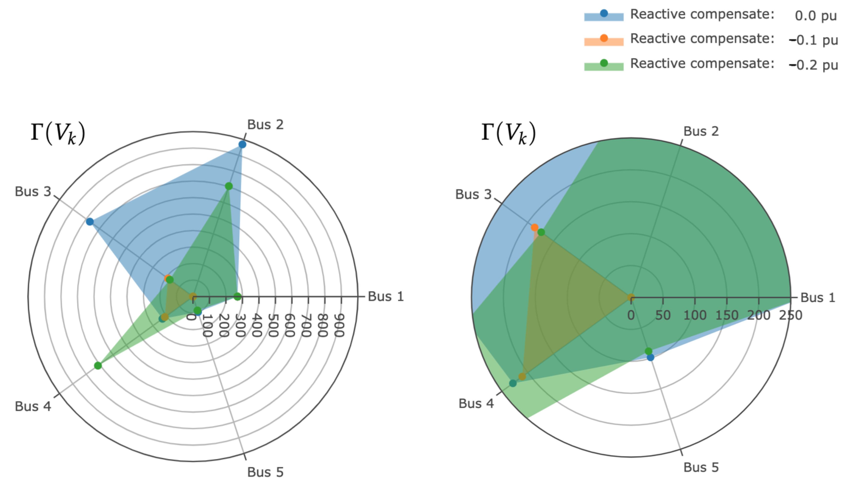
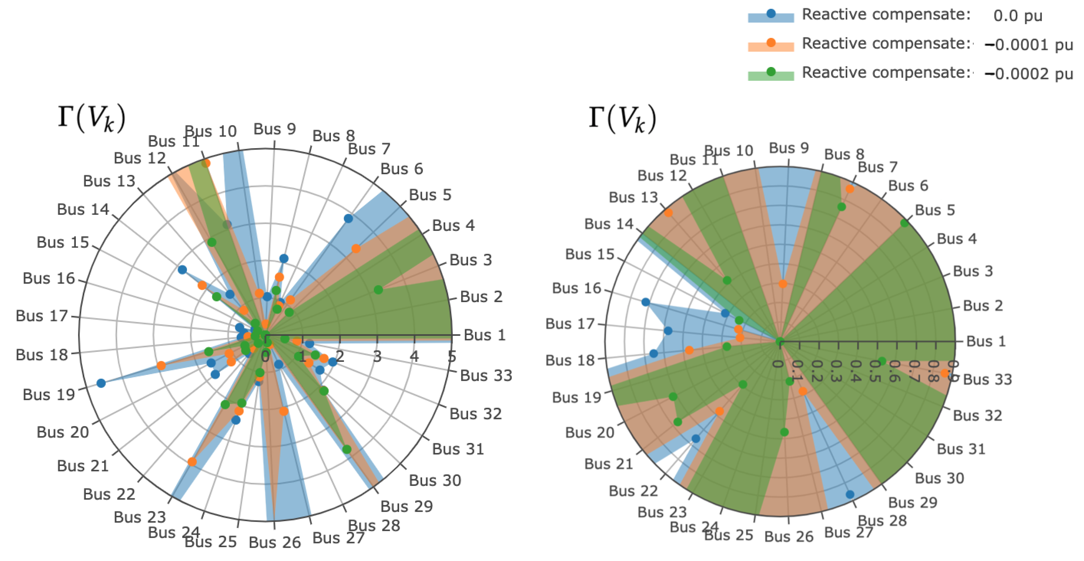
The uncontrollable reactive compensation of RDGs may cause voltage collapse. First, this phenomenon is demonstrated on IEEE 5-bus and IEEE 33-bus test distribution systems, where reactive compensation of generators are assumed. Then, the most vulnerable bus of voltage collapse is investigated.

To demonstrate the effect of reactive compensations of RDGs, the reactive compensation is increasingly applied −0.10 pu and −0.20 pu to the IEEE 5-bus system, and −0.0001 pu and −0.0002 pu to the IEEE 33-bus system. Using the voltage stability indicator, L-index, proposed by [23], the results show that the 5th and 22nd buses of IEEE 5-bus and IEEE 33-bus systems, respectively, are the weakest bus in voltage stability. Next, loading margins show that the 5th bus of IEEE 5-bus and 17th and 18th buses of IEEE 33-bus are the most vulnerable buses of voltage collapse, as shown in

Table 2. Comparisons of first two weakest buses of voltage stability and the most vulnerable bus of voltage collapse on IEEE 5-bus distribution test system.

	Reactive Compensate
	0.00 pu	−0.10 pu	−0.20 pu
the first two weakest buses of voltage stability: ( L-index )	Bus 5, 1	Bus 5, 1	Bus 5, 1
	(0.0029, 0.0017)	(0.0029, 0.0017)	(0.0029, 0.0017)
The highest risk bus of voltage collapse
the first two weakest buses of $\Gamma$: ($\Gamma$)	Bus 5, 4	Bus 5, 1	Bus 1, 5
	(98.58, 228.76)	(233.62, 270.26)	(270.25, 353.36)
The weakest bus of loading margin:	Bus 5 (248 pu)	Bus 5 (248 pu)	Bus 5 (248 pu)

and

Table 3. Comparisons of first two weakest buses of voltage stability and the most vulnerable bus of voltage collapse on IEEE 33-bus distribution test system.

	Reactive Compensate
	0.0000 pu	−0.0001 pu	−0.0002 pu
the first two weakest buses of voltage stability: ( L-index )	Bus 22, 25	Bus 22, 25	Bus 22, 25
	(0.0698, 0.0691)	(0.0699, 0.0692)	(0.0700, 0.0693)
The highest risk bus of voltage collapse
the first two weakest buses of $\Gamma$: ($\Gamma$)	Bus 15, 17	Bus 18, 22	Bus 18, 22
	(0.3174, 0.578)	(0.8216, 0.8567)	(0.9913, 1.0936)
The weakest bus of loading margin:	Bus 18 (0.03 pu)	Bus 17,18 (0.03 pu)	Bus 17 (0.03 pu)

. As a result, the first two weakest buses with the highest possibility of voltage collapse, which are obtained using the minimum value of $\Gamma$ and the loading margin, are almost the same. For the IEEE 5-bus system, the weakest bus in voltage stability is the same with the most vulnerable bus of voltage collapse, as in Table 2.

However, by comparing the results from the loading margin and L-index as given in Table 3, the weakest bus of voltage stability using L-index is not the same with the most vulnerable bus of voltage collapse by the loading margin for the IEEE 33-bus system.

After that, one of the first two weakest buses using $\Gamma$ is verified with loading margin levels of the IEEE 5-bus and 33-bus systems, as shown in Table 2 and Table 3, respectively. The results show that $\Gamma$ can be used for approximating the most vulnerable bus of voltage collapse by considering the different reactive compensation levels. In the following, the $\Gamma$ will be used to formulate the objective function of the optimal placement determination beneficial for keeping voltage stability and safety and being available to consider the reactive power compensated for by generators.

Moreover, we found that reactive compensation increases the voltage collapse risk by considering $\Gamma$, as shown in Figure 2 and Figure 3. Therefore, uncontrollable reactive compensation of RDGs may cause degraded system operation reliability and voltage collapse.

3.5. Reactive Power Compensation Support Margin for Voltage Stability Improvement

According to the previous results, the possibility of voltage collapse of each bus is controlled by the available reactive support $Q_C$, which can be estimated using the proposed formulation of $\Gamma$. The minimum value of $\Gamma$ can be adopted for estimating the most vulnerable bus of voltage collapse. Therefore, the objective function, which is named Reactive Power Compensation Support Margin for Voltage Stability Improvement (QSVS), is proposed subject to the condition of $V_k>V_k^{SNB}$ as

$$\begin{array}{c}\hfill {\mathrm{QSVS}}_k=\underset{\begin{array}{c}{V}^{min}\le V_k\le V^{max},\\ V_k^{SNB}<V_k\end{array}}{min}\left\{\Gamma \left(V_k\right)\right\}\end{array}$$

(17)

At the kth bus, ${\mathrm{QSVS}}_k$ indicates the voltage stability limit with respect to voltage collapse. Therefore, ${\mathrm{QSVS}}_k>0$ means no voltage collapse, and ${\mathrm{QSVS}}_k=0$ means voltage collapse.

Estimating the voltage stability limit of overall systems, the minimum value of ${\mathrm{QSVS}}_k$ over all buses, which indicates the highest possibility of voltage collapse, is used.

$$\mathrm{QSVS}=min\{{\mathrm{QSVS}}_2,{\mathrm{QSVS}}_3,\cdots ,{\mathrm{QSVS}}_N\}$$

(18)

In system operations, the value of the QSVS should be greater than 0 for stable operation. The more the value of the QSVS from 0, the more stable the system and safe from voltage collapse. On the other hand, if the value of QSVS is equal to 0, the voltage collapse will occur and should be avoided for safety in operating.

3.6. Reactive Power Compensation of RDGs

Different types of generators convert natural energy into electricity resulting in non-uniform reactive power compensation. Basically, the reactive compensation of generators is described using the power factor, which is the cosine of the difference between voltage and current phase angles. For simplification, reactive power compensation and active generated power of a RDG are represented using a ratio named reactive power compensation rate (RCR), as follows.

$$\mathrm{RCR}=\frac{Q_{comp}^{RDG}}{P^{RDG}}$$

(19)

where $Q_{comp}^{RDG}$ and $P^{RDG}$ are reactive power compensation of generators and the active power generated by a generator, respectively.

In this paper, the RCR is used for distinguishing the type of RDGs. We assume that for dispatchable-RDG (DP-RDG), the generator is not compensated any reactive power from the system, and RCR is zero. On the other hand, for non-dispatchable RDG (NDP-RDG), the generator’s level of compensated reactive power is assumed to be equal to the generated active power times RCR.

4. Location and Sizing of RDGs Considering Reactive Power Compensation

4.1. Optimal Location of RDGs Considering Reactive Power Compensation

The goal of determining locations of RDGs in distribution systems is to improve voltage stability against uncontrollable reactive compensation. This paper determines the most proper location or the weakest bus by removing load from one bus to another. To specify the buses for which loads are disconnected, we use a vector $(c_2,c_3,\cdots ,c_N)$ where $c_k=0$ means that the load of kth bus is disconnected and $c_k=1$ means otherwise. In addition to the specification of buses whose loads are removed, we treat the peak load factor ($lf$) and the reactive power compensation ratio (RCR) as parameters, and we consider QSVS as a function of these parameters. Finally, the optimal location of RDGs are considered to be the maximization of $\mathrm{QSVS}((c_2,c_3,\cdots ,c_N),lf,\mathrm{RCR})$ over possible choices of vector $(c_2,c_3,\cdots ,c_N)$ as,

$$\underset{(c_2,c_3,\cdots ,c_N)\in \mathcal{C}}{\arg \max }\left\{\mathrm{QSVS}((c_2,c_3,\cdots ,c_N),lf,\mathrm{RCR})\right\}$$

(20)

where $\mathcal{C}$ is a set of all possible binary vectors having the size $N-1$ and the number of 1 s is no smaller than $N-1-N^{RDG}$. The optimization problem given in Equation (20) should be solved being subjected to the following voltage constraint;

$$V^{min}\le V_k\le V^{max};k\in 1,2,\cdots ,N,$$

(21)

where $V^{min}$, $V^{max}$ and $V_k$ are the lower voltage limit, the upper voltage limit, and the voltage of kth bus, respectively.

The algorithm of the RDGs optimal location is given as Algorithm 1.

Algorithm 1: Optimal location for RDGs.

4.2. Methodology for Optimal Size of RDGs

After the optimal location(s) (X from Algorithm 1) of the buses of RDGs is obtained, the optimal sizes of RDGs is determined so as to minimize the power losses ($P_{loss}$), which can be calculated using Equation (2).

$$\underset{\{P_k^{RDG}\in \mathbb{R},k\in X\}}{min}{P}_{loss}(P_k^{RDG},Q_k^{RDG})$$

(22)

The minimization is given in Equation (22) should be solved with being subjected to the following inequality and equality constraints.

• Voltage constraint

The minimum and the maximum voltage constraints given in Equation (21)

2.

RDG size constraint

The active power produced by RDGs should be no larger than the system’s total active power demand because the violation of this constraint results in a reverse power flow in the system. This constraint is expressed as follows.

$$0\le \sum _{k\in X}{P}_k^{RDG}\le \sum _{k=1}^N{P}_k$$

(23)

3.

Voltage collapse constraint

The voltage magnitude at each bus must be grater than its voltage stability limit ($V_k^{SNB}$), since the violation of the constraint results in voltage collapse and system blackout. This constraint is expressed as follows.

$$V_k^{SNB}<V_k$$

(24)

For solving RDG sizing problem, we have adopted a simple exhaustive search with discritizing possible size of RDG as integer multiples of $\frac{P^t}{N_s}$, where $P^t$ is the maximum possible size $P^t={\sum }_{k=1}^N{P}_k$ due to the constraint (23), and $N_s$ is an integral parameter which control the quartization step $\frac{P^t}{N_s}$.

4.3. Overall Design Procedure

In summary, the proposed system design process is described. First, the number of the RDGs and the set of the peak load factors are given. For representing the reactive compensation of RDGs, RCR is given as another input. After the inputs are prepared, the candidate locations of RDGs are determined using Algorithm 1. Then, the optimal sizes of RDGs are determined from the candidate locations by using Algorithm 2. Finally, the optimal solution is chosen by considering the minimum power losses. The flowchart of the proposed system design is shown in Figure 4.

Algorithm 2: Optimal size of RDGs.

5. Simulations

The proposed methodology was implemented using Python programming with a library called PYPSA [29], and simulations were conducted. Simulation 1: optimal location and size without reactive compensation of one and two RDGs. Simulation 2: reactive power compensation test.

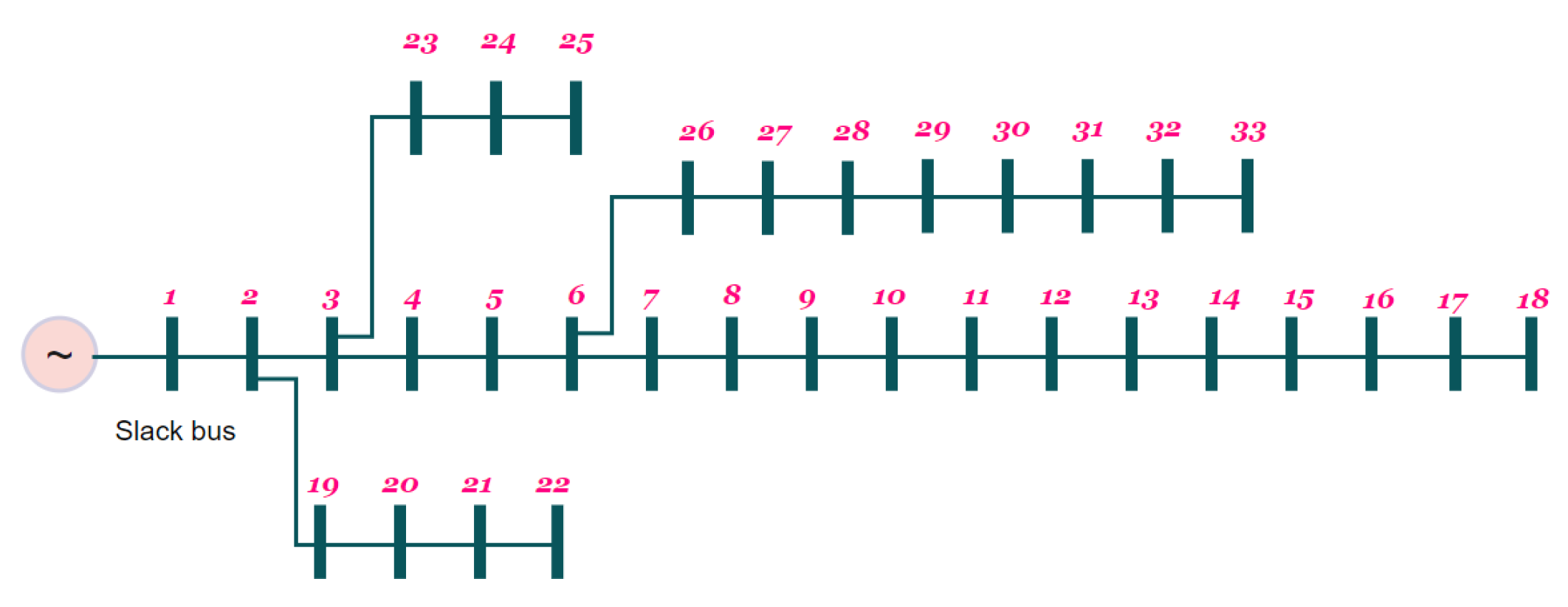
The proposed methodology is applied to the IEEE 33-bus test distribution system, which is shown in Figure 5. The complete system data at the peak load demand are taken from [30]. The details of the system parameters are given in Table A3 and Table A4. This system is supplied from one substation with a total peak load of 3.715 MW and 2.30 MVAr. The total power losses at the peak demand without RDGs integration is 212.95 kW. Considering the requirements of the IEEE standard [31], the lower and upper voltages, $V^{min}$ and $V^{max}$, at the kth bus are set to be 0.95 pu and 1.05 pu, respectively, and the power generating limits of RDGs are equal to total power demand.

5.1. Simulation 1: Optimal Location and Size of RDGs

5.1.1. Location and Size of 1 RDG

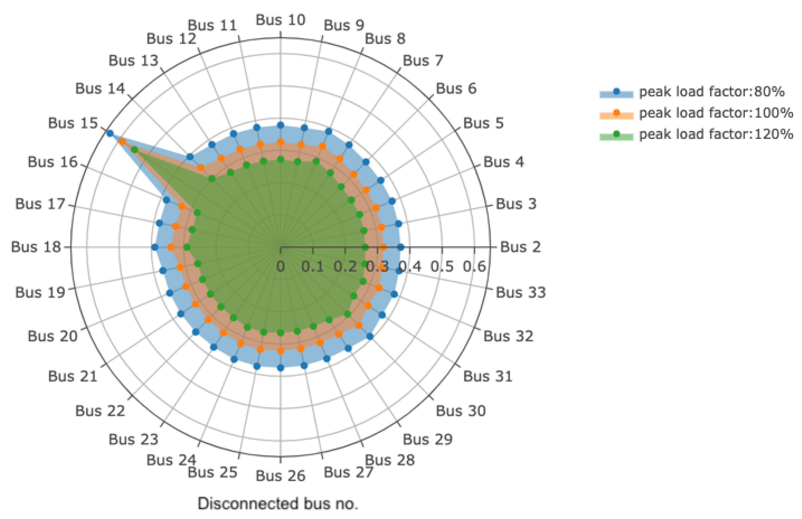
For single RDG installation, first, the candidate location is determined using Algorithm 1. Figure 6 describes the variation of QSVS for load removal from each bus and for each peak load factor. The radius represents the value of QSVS, and the sector represents the individual bus of which load is disconnected. By considering the maximum increment of QSVS with peak load factor 80%, 100% and 120%, the 15th bus is detected as the most vulnerable bus of voltage collapse, and it is the candidate location for a single RDG installation.

Table 4. The candidate location of a single RDG installation for each peak load factor of IEEE33-bus test distribution system using Algorithm 1.

Peak Load Factor	The Disconnected Bus	Maximum Increment of QSVS (%)
80%	15	70.98%
100%	15	85.59%
120%	15	108.31%

shows the maximum increment of QSVS achieved by disconnecting the load from the 15th bus.

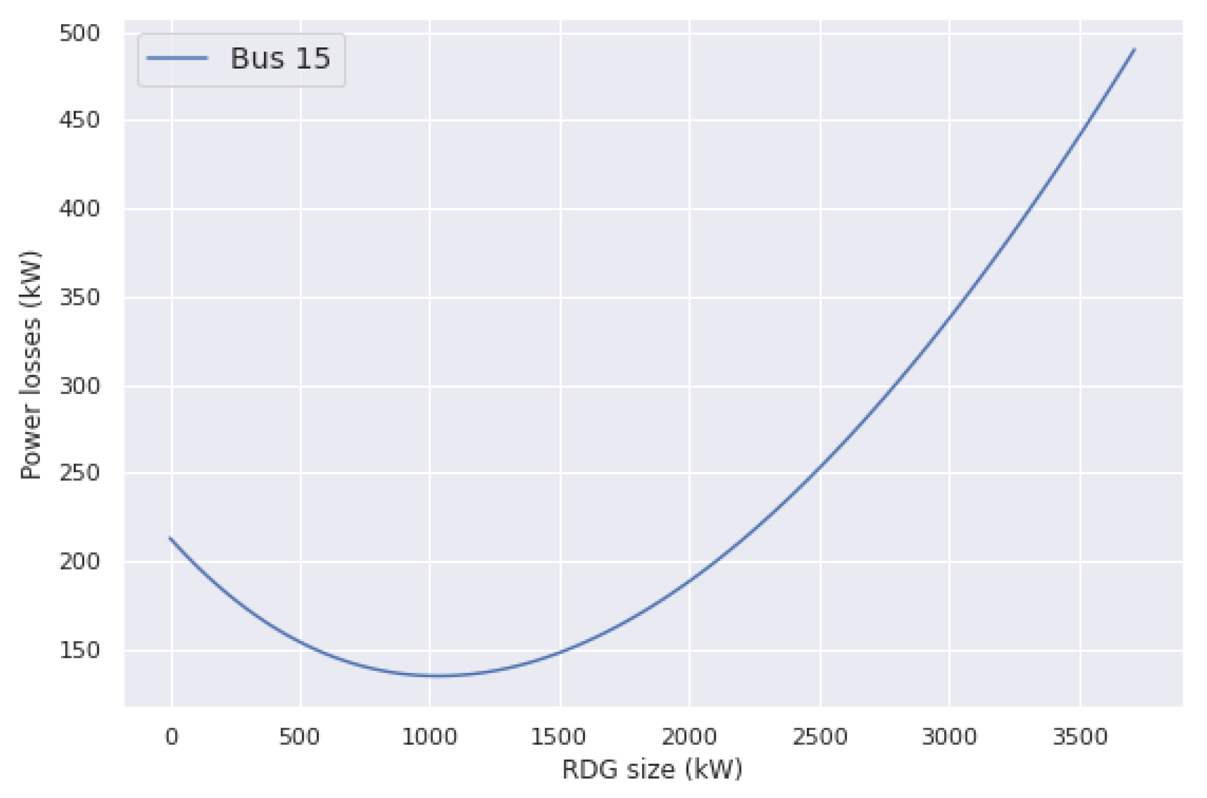
From the minimization of power losses, the optimal size of RDG at the 15th bus is determined using Algorithm 2, the result 1040.20 kW has been obtained as Figure 7 and

Table 5. Results for installing a single RDG on IEEE 33-bus test distribution systems.

Optimal Location (Bus No.)	Optimal Size (kW)	RCR	Power Losses (kW)
			Without	With 1 RDG
15	1040.20	0	212.95	134.71

show the power losses are decreased to 134.71 kW which corresponds to loss reduction 0.0752 per 1 kW generated power of RDG. In addition, in order to check that the result will not distract the supply ability to support demand, the minimum loading margin is demonstrated. The result of the optimal location and size of the single RDG is compared with [10,12,13,19,32,33,34,35] as shown in

Table 6. Comparison results of optimal locations and sizes for installing one RDG of IEEE 33-bus distribution test system (↑:improvement of voltage stability; ↓ degradation of voltage stability; red.: power loss reduction).

Technique	RDG Location	RDG Size	Power Loss (kW)		Voltage Stability	Minimum Loading Margin
	(Bus No.)	(kW)	(kW)	[Red. /1 kW-RDG]	[Max. L-Index]
Without	-	-	212.95	-	0.0698	0.03
GA [32]	6	2580	112.68	0.0389	0.0728↓	0.03
BSOA [33]	8	1857.50	119.81	0.0501	0.0683↑	0.03
PSO [34]	6	3150	116.89	0.0305	0.0752 ↓	0.03
Analytical [10,35]	6	2490	112.83	0.0402	0.0725 ↓	0.03
ALOA [12]	6	2450	112.97	0.0408	0.0724↓	0.03
WOA [13]	30	1542.67	126.92	0.0558	0.0655↑	0.03
MLPSO [19]	6	2420	113.10	0.0413	0.0723↓	0.03
Proposed	15	1040.20	134.71	0.075	0.0691↑	0.03

. As a result, the proposed methodology shows the best power loss reduction per 1 kW generated power of the single RDG with voltages stability improvement.

5.1.2. Locations and Sizes of 2 RDGs

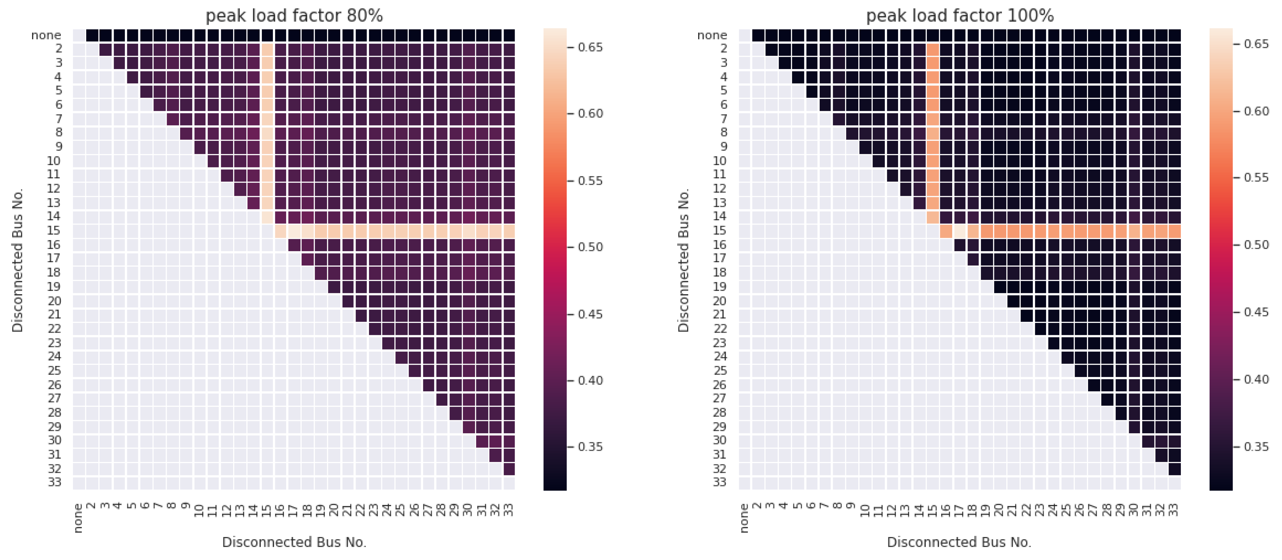
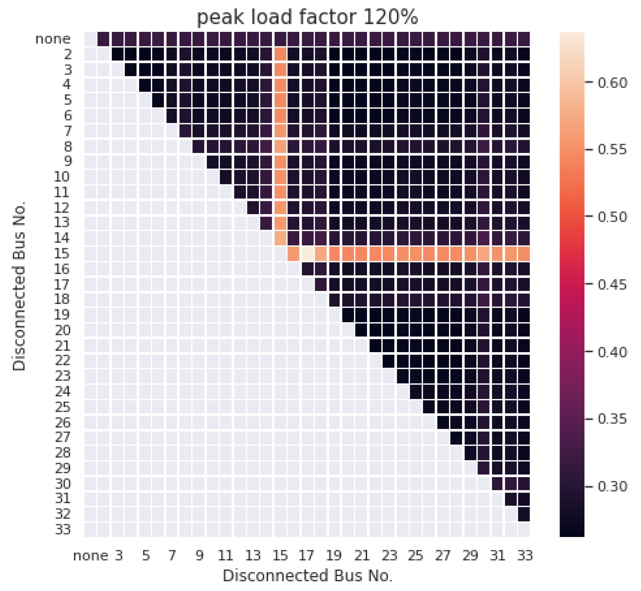
For two RDGs’ installation, first, the candidate locations are determined using Algorithm 1. Figure 8 describes the variation of QSVS for load removal from pair of buses and for each peak load factor. The colors represent the values of QSVS. By considering the maximum increment of QSVS with $lf$ 80% 100% and 120%, buses 15th and 17th are detected as the most vulnerable buses of voltage collapse in

Table 7. The candidate locations of two RDGs installation for each peak load factor of IEEE33-bus test distribution system using Algorithm 1.

Peak Load Factor	The Disconnected Bus	Maximum Increment of QSVS
80%	15, 17	109.22%
100%	15, 17	108.31%
120%	15, 17	100.71%

and are considered to be the candidate locations for two RDGs installations.

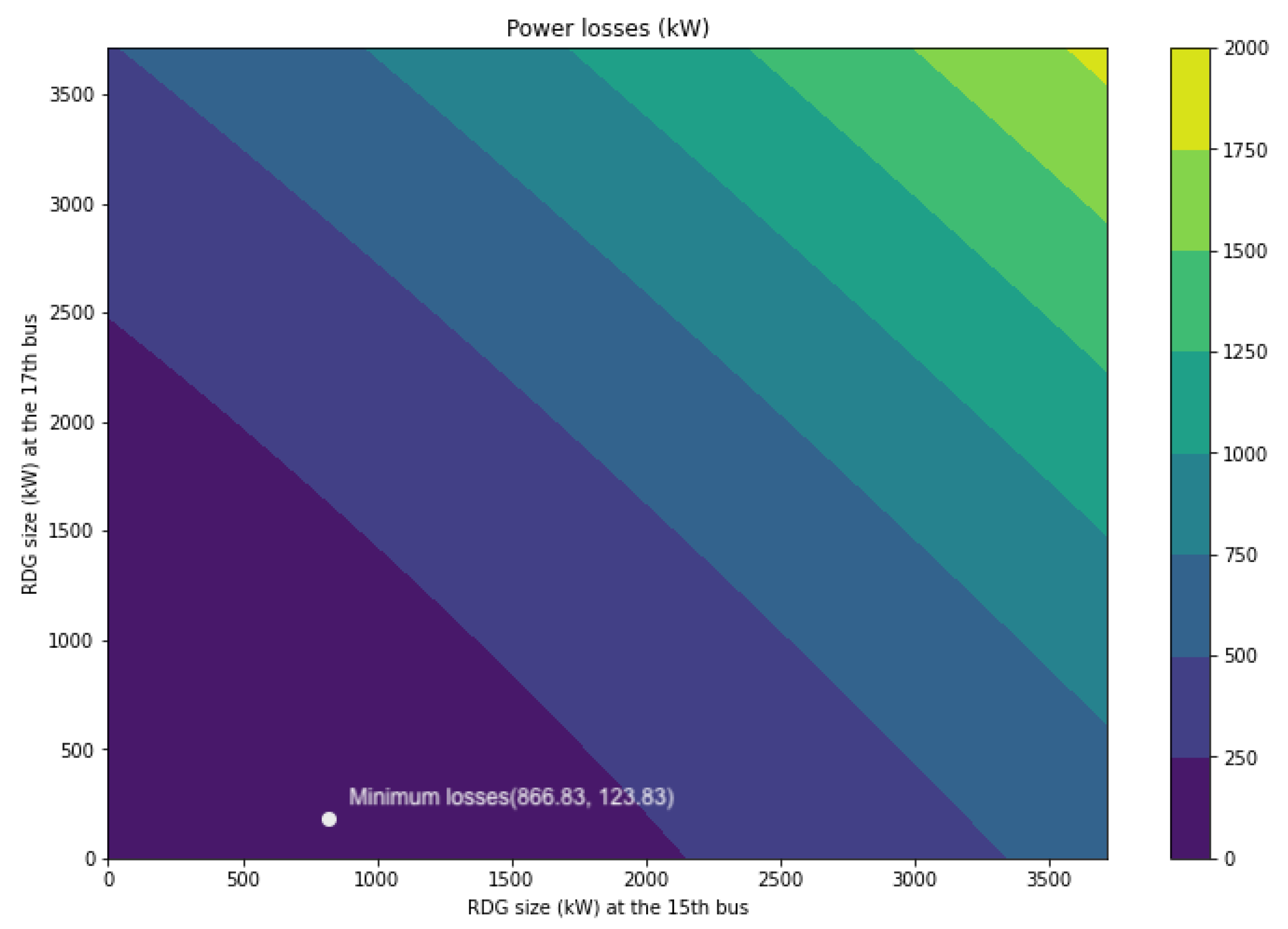
By considering the minimization of power losses in Algorithm 2, the 15th and 17th buses are chosen with sizes of 866.83 and 123.83 kW, respectively, as given in Figure 9 and

Table 8. Result for installing two RDGs of IEEE 33-bus distribution test system.

Optimal Location [Bus No.]	Optimal Size (kW)	RCR	Power Loss (kW)
			without	with 2 RDGs
15, 17	866.83, 123.83	0	212.95	134.42

. The power losses are decreased down from 212.95 to 134.42 kW which corresponds to loss reduction 0.0793 per 1 kW generated power of two RDGs. The optimal location and size of two RDGs are compared with [10,12,19,32,33,34] in

Table 9. Comparison results of optimal locations and sizes for installing two RDGs of IEEE 33-bus distribution test system (↑: improvement of voltage stability; ↓ degradation of voltage stability; red.: power loss reduction).

Technique	RDG Location	RDG Size	Power Loss (kW)		Voltage Stability	Minimum Loading Margin
	[Bus No.]	(kW)	(kW)	[Red./1 kW-RDG]	[Max. L-Index]
-	without	-	212.95	-	0.0698	0.03
GA [32]	13	837.5	88.00	0.0610	0.0687↑	0.03
	29	1212.2
BOSA [33]	13	880	90.05	0.0681	0.0676↑	0.03
	31	924
PSO [19,34]	11	2420	171.53	0.0123	0.0733↓	0.04
	31	960
ALOA [12]	13	850	87.80	0.0613	0.0655↑	0.03
	30	1191.1
MLPSO [19]	13	820	87.76	0.0635	0.0654↑	0.03
	30	1150
Proposed	15	866.83	134.42	0.0793	0.0681↑	0.03
	17	123.83

, and it is shown the proposed methodology shows the best power loss reduction per 1 kW generated power of the two RDGs with voltages stability improvement.

5.2. Simulation 2: Reactive Power Compensation Test

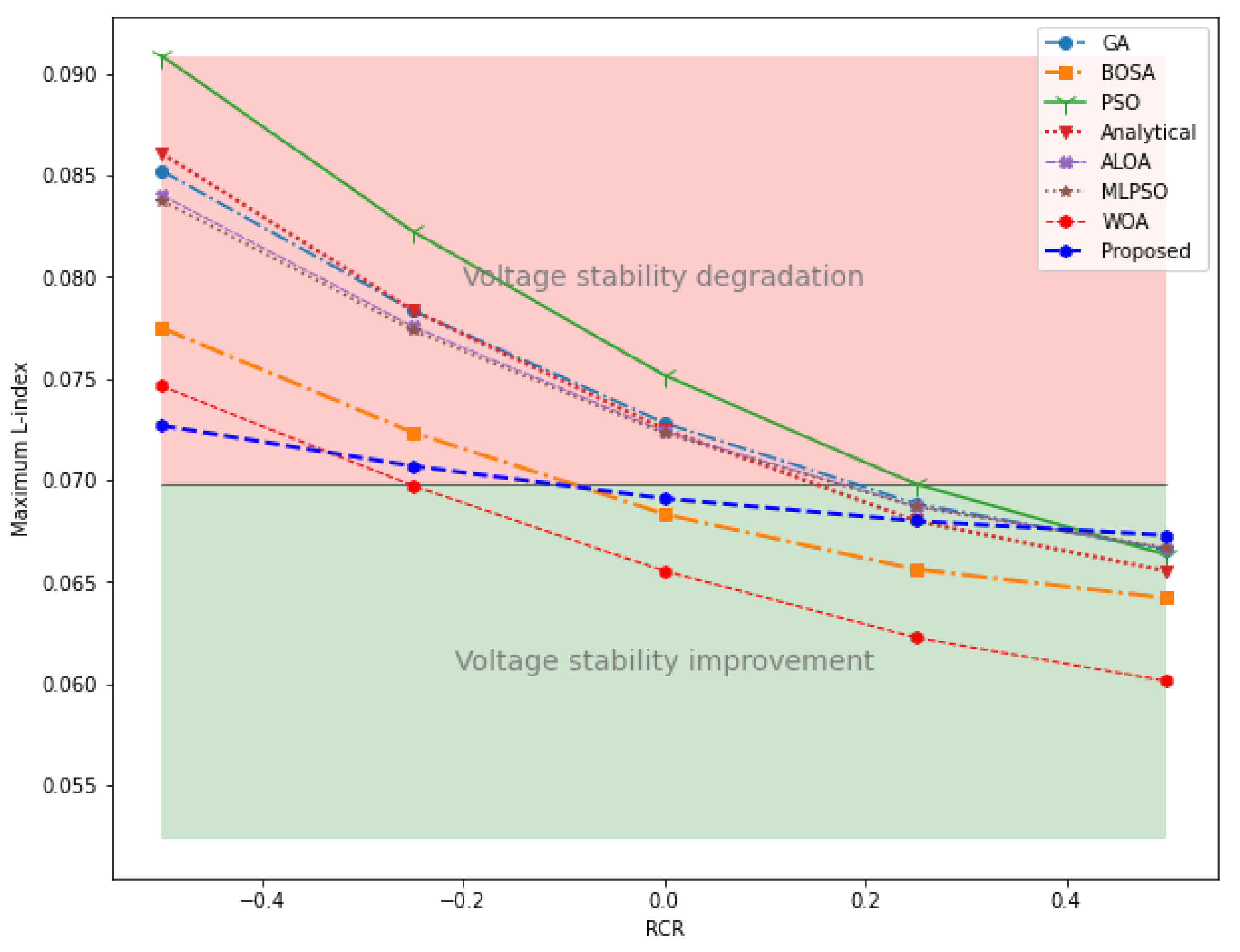
Uncontrollable reactive power compensation of RDGs is a hypothetical factor as for the voltage stability degradation. To simulate this effect, the reactive power compensation ratio (RCR) has been introduced with sample values, i.e., RCR = 0 for DP-RDGs, RCR = ±0.25 and ±0.5 for NDP-RDGs, and maximum L-index has been compared among different installations of RDG(s) with individual RCR value.

Table 10. Result for installing one RDG of IEEE 33-bus distribution test system with the different reactive compensation (↑: improvement of voltage stability; ↓: degradation of voltage stability).

Technique	RDG Location	RDG Size	Voltage Stability [Max. L-Index]
	(Bus No.)	(kW)	RCR = −0.5	RCR = −0.25	RCR = 0.0	RCR = 0.25	RCR = 0.5
Without	-	-	0.0698
GA [32]	6	2580	0.0852↓	0.0784↓	0.0728↓	0.0689↑	0.0666↑
BSOA [33]	8	1857.5	0.0775↓	0.0724↓	0.0683↑	0.0656↑	0.0642↑
PSO [34]	6	3150	0.0822↓	0.0823↓	0.0752↓	0.0698↓	0.0663↑
Analytical [10,35]	6	2490	0.0861↓	0.0784↓	0.0725↓	0.0680↑	0.0655↑
ALOA [12]	6	2450	0.0840↓	0.0776↓	0.0724↓	0.0687↑	0.0667↑
WOA [13]	30	1542.67	0.0746↓	0.0697↑	0.0655↑	0.0623↑	0.0601↑
MLPSO [19]	6	2420	0.0838↓	0.0774↓	0.0723↓	0.0687↑	0.0667↑
Proposed	15	1040.20	0.0727↓	0.0707↓	0.0691↑	0.0680↑	0.0673↑

and Figure 10 show the comparison result for one RDG installation, and

Table 11. Result for installing two RDGs of IEEE 33-bus distribution test system with three different RCRs (↑: improvement of voltage stability; ↓: degradation of voltage stability).

Technique	RDG Location	RDG Size	Voltage Stability (L-Index)
	(Bus No.)	(kW)	$\mathbf{RCR}$ = −0.5	$\mathbf{RCR}$ = −0.25	$\mathbf{RCR}$ = 0.0	$\mathbf{RCR}$ = 0.25	$\mathbf{RCR}$ = 0.5
Without	-	-	0.0698
GA [32]	13	837.5	0.0792↓	0.0733↓	0.0687↑	0.0655↑	0.0637↑
	29	1212.2
BOSA [33]	13	880	0.0792↓	0.0717↓	0.0676↑	0.0649↑	0.0634↑
	31	924
PSO [19,34]	11	2420	0.0768↓	0.0818↓	0.0733↓	0.0669↑	0.0626↑
	31	960
ALOA [12]	13	850	0.0775↓	0.0710↓	0.0655↑	0.0613↑	0.0585↑
	30	1191.1
MLPSO [19]	13	820	0.0782↓	0.0725↓	0.0680↑	0.0649↑	0.0633↑
	15	1114.5
Proposed	15	866.83	0.0717↓	0.0697↑	0.0681↑	0.0671↑	0.0664↑
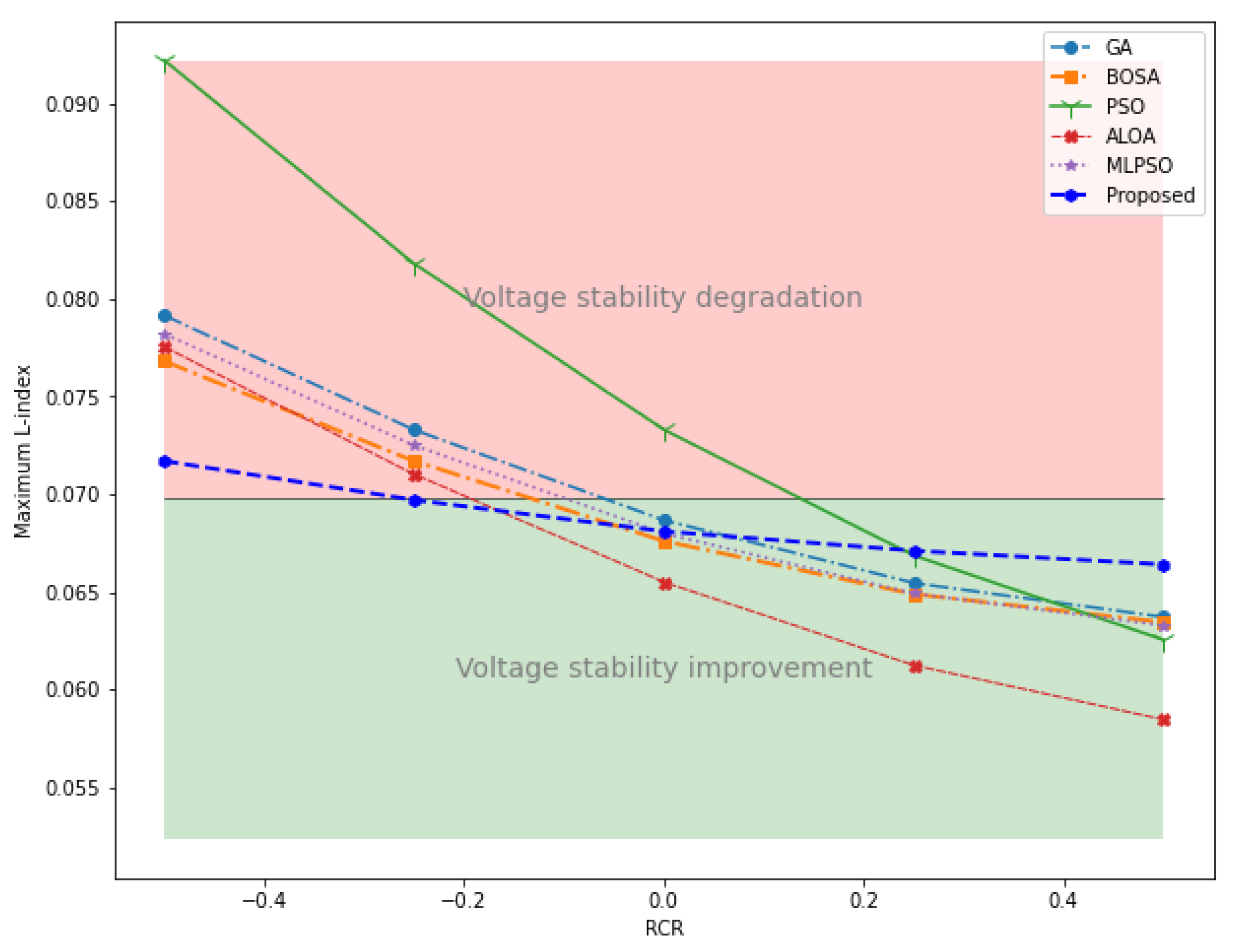
	17	123.83

and Figure 11 show the result for the case of two RDGs installation.

By considering the variation of voltage stability from Table 10 and Figure 10, we found that the proposed methodology provides the best result in the robustness of voltage stability against the uncontrollable reactive compensation.

Similarly, by considering the variation of voltage stability from Table 11 and Figure 11, we found that the proposed methodology provides the best result in the robustness of voltage stability against the uncontrollable reactive compensation.

5.3. Observations

• By considering the voltage stability and the power losses reduction individually, we found that the maximum power losses reduction does not provide maximum voltage stability, especially when reactive compensations occur.
• The simulations show the best result in improving voltage stability by maximizing the increment of QSVS which estimates the voltage collapse margin. Therefore, the voltage stability is dependent on the voltage collapse margin. However, the most vulnerable bus of voltage collapse can not be indicated directly by using voltage stability indicators such as the L-index.
• The results clearly show that the reactive compensation affects the voltage stability of the distribution systems. Therefore, generators’ uncontrollable reactive compensation and reactive support’s ability need to be accountable for considering voltage stability.
• The vulnerable bus of voltage collapse in peak load situations is more apparent than the lower peak demand.

6. Concluding Remarks

In this paper, the voltage-reactive power margin with respect to voltage collapse ($\Gamma$) and the optimal location of RDG installation, which maximize the minimum $\Gamma$, have been proposed. The proposed methodology for determining locations and sizes of RDGs emphasizes the voltage stability against uncontrollable reactive power compensation. The effectiveness of the suggested approach is verified by using the different possible ratios of reactive power compensation (RCR) on the IEEE 33-bus test distribution system. The results were compared with those obtained using other algorithms to investigate the effectiveness in terms of voltage stability. It is obvious from the comparison that the proposed approach provides a notable performance in terms of maximum power losses reduction. Moreover, our results maintain the robustness of voltage stability against variable reactive power compensation.

References

1. Floyd, J.; Zubevich, K. Linking foresight and sustainability: An integral approach. Futures 2010, 42, 59–68. [Google Scholar] [CrossRef]
2. Luna-Rubio, R.; Trejo-Perea, M.; Vargas-Vázquez, D.; Ríos-Moreno, G.J. Optimal sizing of renewable hybrids energy systems: A review of methodologies. Sol. Energy 2012, 86, 1077–1088. [Google Scholar] [CrossRef]
3. Xu, F.L.; Zhao, S.S.; Dawson, R.W.; Hao, J.Y.; Zhang, Y.; Tao, S. A triangle model for evaluating the sustainability status and trends of economic development. Ecol. Model. 2006, 195, 327–337. [Google Scholar] [CrossRef]
4. Hadjsaid, N.; Canard, J.; Dumas, F. Dispersed generation impact on distribution networks. IEEE Comput. Appl. Power 1999, 12, 22–28. [Google Scholar] [CrossRef]
5. Barker, P.P.; De Mello, R.W. Determining the impact of distributed generation on power systems. I. Radial distribution systems. In Proceedings of the 2000 Power Engineering Society Summer Meeting (Cat. No.00CH37134), Seattle, WA, USA, 16–20 July 2000; Volume 3, pp. 1645–1656. [Google Scholar] [CrossRef]
6. Pepermans, G.; Driesen, J.; Haeseldonckx, D.; Belmans, R.; D’haeseleer, W. Distributed generation: Definition, benefits and issues. Energy Policy 2005, 33, 787–798. [Google Scholar] [CrossRef]
7. Ackermann, T.; Andersson, G.; Söder, L. Distributed generation: A definition. Electr. Power Syst. Res. 2001, 57, 195–204. [Google Scholar] [CrossRef]
8. Dalton, G.J.; Lockington, D.A.; Baldock, T.E. Case study feasibility analysis of renewable energy supply options for small to medium-sized tourist accommodations. Renew. Energy 2009, 34, 1134–1144. [Google Scholar] [CrossRef]
9. Yilmaz, P.; Hakan Hocaoglu, M.; Konukman, A.E.S. A pre-feasibility case study on integrated resource planning including renewables. Energy Policy 2008, 36, 1223–1232. [Google Scholar] [CrossRef]
10. Gözel, T.; Hocaoglu, M.H. An analytical method for the sizing and siting of distributed generators in radial systems. Electr. Power Syst. Res. 2009, 79, 912–918. [Google Scholar] [CrossRef]
11. Khatod, D.K.; Pant, V.; Sharma, J. Evolutionary programming based optimal placement of renewable distributed generators. IEEE Trans. Power Syst. 2013, 28, 683–695. [Google Scholar] [CrossRef]
12. Ali, E.S.; Abd Elazim, S.M.; Abdelaziz, A.Y. Optimal allocation and sizing of renewable distributed generation using ant lion optimization algorithm. Electr. Eng. 2018, 100, 99–109. [Google Scholar] [CrossRef]
13. Dinakara Prasad Reddy, P.; Veera Reddy, V.C.; Gowri Manohar, T. Optimal renewable resources placement in distribution networks by combined power loss index and whale optimization algorithms. J. Electr. Syst. Inf. Technol. 2018, 5, 175–191. [Google Scholar] [CrossRef]
14. Hung, D.Q.; Mithulananthan, N.; Lee, K.Y. Optimal placement of dispatchable and nondispatchable renewable DG units in distribution networks for minimizing energy loss. Int. J. Electr. Power Energy Syst. 2014, 55, 179–186. [Google Scholar] [CrossRef]
15. HassanzadehFard, H.; Jalilian, A. Optimal sizing and location of renewable energy based DG units in distribution systems considering load growth. Int. J. Electr. Power Energy Syst. 2018, 101, 356–370. [Google Scholar] [CrossRef]
16. Chang, R.W.; Mithulananthan, N.; Saha, T.K. Novel mixed-integer method to optimize distributed generation mix in primary distribution systems. In Proceedings of the AUPEC 2011, Brisbane, Australia, 25–28 September 2011; pp. 1–6. [Google Scholar]
17. Fazliana Abdul Kadir, A.; Mohamed, A.; Shareef, H.; Asrul Ibrahim, A.; Khatib, T.; Elmenreich, W. An improved gravitational search algorithm for optimal placement and sizing of renewable distributed generation units in a distribution system for power quality enhancement. J. Renew. Sustain. Energy 2014, 6, 1–18. [Google Scholar] [CrossRef]
18. Milovanović, M.; Tasić, D.; Radosavljević, J.; Perović, B. Optimal Placement and Sizing of Inverter-Based Distributed Generation Units and Shunt Capacitors in Distorted Distribution Systems Using a Hybrid Phasor Particle Swarm Optimization and Gravitational Search Algorithm. Electr. Power Components Syst. 2020, 48, 543–557. [Google Scholar] [CrossRef]
19. Karunarathne, E.; Pasupuleti, J.; Ekanayake, J.; Almeida, D. Optimal Placement and Sizing of DGs in Distribution Networks Using MLPSO Algorithm. Energies 2020, 13, 6185. [Google Scholar] [CrossRef]
20. Naderipour, A.; Nowdeh, S.A.; Saftjani, P.B.; Abdul-Malek, Z.; Bin Mustafa, M.W.; Kamyab, H.; Davoudkhani, I.F. Deterministic and probabilistic multi-objective placement and sizing of wind renewable energy sources using improved spotted hyena optimizer. J. Clean. Prod. 2021, 286, 124941. [Google Scholar] [CrossRef]
21. Awad, A.; Abdel-Mawgoud, H.; Kamel, S.; Ibrahim, A.A.; Jurado, F. Developing a Hybrid Optimization Algorithm for Optimal Allocation of Renewable DGs in Distribution Network. Clean Technol. 2021, 3, 409–423. [Google Scholar] [CrossRef]
22. Cutsem, T.V.; Vournas, C. Voltage Stability of Electric Power Systems; Springer: Boston, MA, USA, 1998. [Google Scholar]
23. Kessel, P.; Glavitsch, H. Estimating the Voltage Stability of a Power System. IEEE Trans. Power Deliv. 1986, 1, 346–354. [Google Scholar] [CrossRef]
24. Hung, D.Q.; Mithulananthan, N. Multiple distributed generator placement in primary distribution networks for loss reduction. IEEE Trans. Ind. Electron. 2013, 60, 1700–1708. [Google Scholar] [CrossRef]
25. Greene, S.; Dobson, I.; Alvarado, F. Sensitivity of the loading margin to voltage collapse with respect to arbitrary parameters. IEEE Trans. Power Syst. 1997, 12, 262–272. [Google Scholar] [CrossRef] [Green Version]
26. Hosseinzadeh, N.; Aziz, A.; Mahmud, A.; Gargoom, A.; Rabbani, M. Voltage stability of power systems with renewable-energy inverter-based generators: A review. Electronics 2021, 10, 115. [Google Scholar] [CrossRef]
27. Shuai, Z.; Peng, Y.; Liu, X.; Li, Z.; Guerrero, J.M.; Shen, Z.J. Parameter Stability Region Analysis of Islanded Microgrid Based on Bifurcation Theory. IEEE Trans. Smart Grid 2019, 10, 6580–6591. [Google Scholar] [CrossRef]
28. Chakrabarti, S. Notes on Power System Voltage Stability. Dept. of EE, IIT, Kanpur 2011. Available online: https://home.iitk.ac.in/~saikatc/EE632_files/VS_SC.pdf (accessed on 22 April 2021).
29. Brown, T.; Hörsch, J.; Schlachtberger, D. PyPSA: Python for Power System Analysis. arXiv 2018, arXiv:1707.09913. [Google Scholar] [CrossRef] [Green Version]
30. Baran, M.; Wu, F. Network reconfiguration in distribution systems for loss reduction and load balancing. IEEE Trans. Power Deliv. 1989, 4, 1401–1407. [Google Scholar] [CrossRef]
31. IEEE Std C57.15-1999; IEEE Standard Requirements, Terminology, and Test Code for Step-Voltage Regulators. IEEE: Piscataway, NJ, USA, 2000; pp. 1–80. [CrossRef]
32. Hassan, A.A.; Fahmy, F.H.; Nafeh, A.E.S.A.; Abu-elmagd, M.A. Genetic single objective optimisation for sizing and allocation of renewable DG systems. Int. J. Sustain. Energy 2017, 36, 545–562. [Google Scholar] [CrossRef]
33. Optimal allocation of multi-type distributed generators using backtracking search optimization algorithm. Int. J. Electr. Power Energy Syst. 2015, 64, 1197–1205. [CrossRef]
34. Kansal, S.; Kumar, V.; Tyagi, B. Optimal placement of different type of DG sources in distribution networks. Int. J. Electr. Power Energy Syst. 2013, 53, 752–760. [Google Scholar] [CrossRef]
35. Acharya, N.; Mahat, P.; Mithulananthan, N. An analytical approach for DG allocation in primary distribution network. Int. J. Electr. Power Energy Syst. 2006, 28, 669–678. [Google Scholar] [CrossRef]
36. Gouda, P.K.; Sahoo, A.K.; Hota, P.K. Optimal power flow including unified power flow controller in a deregulated environment. Int. J. Appl. Eng. Res. 2015, 10, 505–522. Available online: https://www.researchgate.net/publication/282271461_Optimal_power_flow_including_unified_power_flow_controller_in_a_deregulated_environment (accessed on 7 May 2021).
Figure 1. An example of reactive support variation at different voltage levels with parameter description for estimating vulnerable buses of voltage collapse.
Energies 15 02126 g001
Figure 2. The variation of Γ indicating voltage collapse risk on IEEE 5-bus test distribution system.
Energies 15 02126 g002
Figure 3. The variation of Γ indicating voltage collapse risk on IEEE 33-bus test distribution system.
Energies 15 02126 g003
Figure 4. A flowchart of the proposed method.
Energies 15 02126 g004
Figure 5. Single line diagram of the 33-bus test distribution system.
Energies 15 02126 g005
Figure 6. Variation of QSVS for load removal from each bus and for each peak load factor on IEEE 33-bus test distribution system.
Energies 15 02126 g006
Figure 7. Variation of power losses with a single RDG for the IEEE 33-bus test distribution system.
Energies 15 02126 g007
Figure 8. Variation of QSVS at each removal loads and for each peak load factors on IEEE 33-bus test distribution system.
Energies 15 02126 g008aEnergies 15 02126 g008b
Figure 9. Variation of power losses with two RDGs for the IEEE 33-bus test distribution system.
Energies 15 02126 g009
Figure 10. Variation of voltage stability with reactive compensations of 1 RDG using maximum L-index.
Energies 15 02126 g010
Figure 11. Variation of voltage stability with reactive compensations of 2 RDGs using maximum L-index.
Energies 15 02126 g011