Forecasting Daily Electricity Consumption in Thailand Using Regression, Artificial Neural Network, Support Vector Machine, and Hybrid Models

Abstract

This article involves forecasting daily electricity consumption in Thailand. Electricity consumption data are provided by the Electricity Generating Authority of Thailand, the leading power utility state enterprise under the Ministry of Energy. Five forecasting techniques, including multiple linear regression, artificial neural network (ANN), support vector machine, hybrid models, and ensemble models, are implemented. The article proposes a hyperparameter tuning technique, called sequential grid search, which is based on the widely used grid search, for ANN and hybrid models. Auxiliary variables and indicator variables that can improve the models’ forecasting performance are included. From the computational experiment, the hybrid model of a multiple regression model to forecast the expected daily consumption and ANNs from the sequential grid search to forecast the error term, along with additional indicator variables for some national holidays, provides the best mean absolution percentage error of 1.5664% on the test data set.

1. Introduction

Forecasting electricity consumption plays an important role in planning for electricity generation capacity and required resources. Accurate electricity consumption forecasting can reduce the risk of power outage and reduce excess electricity generation. Avoiding power outage is essential for economic growth as the electricity is a main source of energy for industries. The low excess electricity generation can save the generating cost and reduce emissions in environment. Time intervals in electricity generation capacity planning vary from a unit-load period (30-min interval), daily, monthly, and yearly consumption. For power plant capacity, a long-term yearly forecast up to 20 years is performed. Intermediate-term time interval forecasts, e.g., monthly, in the span of three to five years, is required for fuel supply and maintenance planning. Short-term forecasts in unit-load, daily, and weekly intervals are made for the efficient daily operation of the electricity power plants [1].

Traditionally, statistical models, such as multiple linear regression (MLR), triple exponential smoothing (Holt–Winters) model, have been used to forecast electricity demand. MLR in particular remains to be the basic model to forecast energy load in recent studies. Vu et al. performed monthly electricity demand forecast in the state of New South Wales, Australia [2]. The model contains average values of the following variables: cooling degree days, heating degree days, rainfall, wind speed, sunshine hours, solar exposure, evaporation, humidity percentage, maximum temperature, and minimum temperature, the total number of clear days, cloudy, and rainy in a month, as well as electricity price, population size, and gross state product (GSP). Amber et al. developed an MLR model to forecast daily electricity consumption in two buildings of London South Bank University [3]. The model contains six input variables: ambient temperature, solar radiation, relative humidity, wind speed, weekday index, and building type. Among them, temperature, weekday index, and building type are significant. The model performance is measured using the normalized root mean square error. The models can achieve 12–13% forecast errors for the two buildings. Dudic et al. performed monthly and yearly electricity consumption forecasting for the German power market using MLR [4]. Independent variables are monthly average temperature (measured in 10 different locations in Germany), an auxiliary variable representing air conditioning usage that is computed as average temperature subtracting 17 degrees Celsius, Germany’s monthly industrial production based on Eurostat data, number of days in a month, annual GDP, and an electricity efficiency variable.

In the last decade, machine learning models have emerged as effective forecasting models for energy consumption [5]. ML models are widely used to forecast electricity consumption in different applications as the models can deal with non-linear patterns in the energy consumption data [6]. Yuan et al. developed an artificial neural network (ANN) as a prediction model for the seasonal hourly electricity consumption for a university campus in Japan [7]. The model contains the following key input variables: day of the week, hour of the day, hourly dry-bulb temperature, hourly relative humidity, hourly global irradiance, and previous hourly electricity consumption. The model achieves the coefficient of determination (R²) of 96–99% for the training set and 95–99% for the test set. Liu et al. forecasted the daily average load of Chinese cities using the historical data of loads, relative humidity, daily average loads, and somatosensory temperature as input variables [8]. The stacked denoising auto-encoder (SDAE) neural network is developed and compared with the back propagation (BP) neural network. A support vector machine (SVM), another widely used ML model, is implemented to predict five-minute-ahead electricity consumption in the New South Wales region, Australia [9]. Chen et al. developed a support vector regression (SVR) to calculate the electricity demand response baseline of office buildings [10].

Moreover, hybrid models, which are combinations of statistical models and ML models, or combinations of various ML models, are reported to provide a more accurate forecast than using only one machine learning technique. For energy consumption applications, Gonzáles-Romera et al. proposed a hybrid approach that combines a Fourier series forecast of periodic behavior and a neural network to forecast the trend for monthly electricity consumption forecasting in Spain [11]. Fan et al. proposed a hybrid EMD-SVR-AR (empirical mode decomposition, SVR, auto-regressive) model to forecast 30-min unit load of New South Wales, Australia [12]. The proposed model is compared to other models, and is found to outperform four other models, namely the original SVR, PSO-SVR (particle swarm optimization, SVR) hybrid, PSO-BP (particle swarm optimization, back propagation neural network), and AFCM (adaptive fuzzy combination model). Deb et al. provided a comprehensive review on time series forecasting techniques for energy consumption of buildings [13]. The models include ANN, ARIMA, SVM, case-based reasoning (CBR), fuzzy time series model, Grey prediction model, moving average (MA) and exponential smoothing (ES), K-nearest neighbor (KNN) model, and many hybrid models. In addition, Ma and Zhai developed a hybrid WT-SA-FFANN (wavelet transform, simulated annealing, feed forward ANN) model to predict one-day-ahead electricity consumption in Beijing, China [14]. The model uses 24-h electricity load, 24-h lagged and 168-hlagged loads, temperature, humidity, hour of the day, day of the week, and an indicator variable indicating holiday or weekends. Recently, Javed et al. presented a comprehensive analysis that compares forecasting models for a real-time 15-min electricity load of the city of Lahore, Pakistan. Results from computational experiment indicated that the best model among many ML models tested is ANN whose weights are updated using the Levenberg–Marquardt (LM) algorithm [15]. Bento et al. performed a 24-h-ahead, load forecasting using the well-known New England case study. The proposed hybrid model combines a number of ARIMA forecasters with a deep feedforward neural network (DFNN). The DFNN component utilizes forecast values from 15 ARIMA models as input data, along with six lagged values of load data, and some additional variables that indicates the hour of the day, weekday, holiday, and season of the year. Computational study results indicate that the proposed DFNN outperform other standard models, including the regression-support vector machine (R-SVM) and neural network models in terms of the mean absolute percentage error (MAPE) and the root mean square error (RMSE) [16]. Phyo and Jeenanunta developed a hybrid of classification and regression tree (CART) and deep belief network (DBN) to forecast daily load from previous day load and some indicator variables [17].

Besides the forecasting models, input variables significantly affect the accuracy of the forecast. Input variables used for energy forecasting generally are divided into historical data, weather-related variables, time, socioeconomic, and demographics variables [18]. Popular input variables are historical data of electricity consumption, ambient temperature, and time index, such as month, weekday [19].

Different ML models have different set of hyperparameters. Another important factor that is highly related to model performance in terms of forecasting accuracy is the model’s hyperparameter tuning [20]. There are several approaches to tuning hyperparameters, such as grid search (GS), random search, and Bayesian optimization. Zhang et al. employed grid search to fine-tune SVM for short-term wind power prediction [21]. Menapace et al. performed grid search as a hyperparameter tuning method of ANN for predicting hourly drinking water demand [22]. Ribeiro et al. used grid search to tune hyperparameters of the proposed extreme gradient boosting model, and other ML models to forecast one-hour, 12-h, and 24-h-ahead energy consumption past consumption data [23].

Mantovani et al. studied the effectiveness of random search in tuning SVM based on 70 different datasets [24]. Nguyen et al. developed a Bayesian optimization for the hyperparameter tuning of different ML models to predict surface roughness in a polycarbonate manufacturing process [25]. Among them, GS is the simplest method as it evaluates a model’s forecasting performance in all possible combinations of hyperparameter values. In addition to model hyperparameters, another important aspect is the model architecture. Some ML models’, such as the artificial neural network (ANN), architecture is referred to the number of hidden layers and the number of neurons in each layer. For traditional feed-forward ANN, it is common to have one hidden layer [26]. Regarding the number of neurons (or hidden nodes), too many may cause the problem of overfitting, i.e., the model performs well for the training data and performs poorly for the unseen test data, whereas too few may result in underfitting. To set the number of hidden nodes, Sheela and Deepa proposed a trial-and-error approach, which can be performed in a forward or backward manner [27]. The forward approach begins with a small number of hidden nodes and gradually increases the number of nodes until the model performance cannot be further improved. On the other hand, the backward approach starts with a large number of nodes and proceeds by reducing the number of hidden nodes until the optimal number of hidden nodes is found.

This article involves forecasting short-term (daily) electricity consumption. Three well-known individual forecasting models, including the multiple linear regression model, and two ML models, namely, the ANN and support vector machine (SVM), are constructed. To optimize the forecasting performance of ANN and SVM, their hyperparameters are tuned using grid search. In particular, ANN, which has multiple hyperparameters as well as the issue of model architecture to consider, is tuned using the sequential grid search proposed in this article. In addition, hybrid models of MLR and ANN, and of MLR and SVM, as well as ensemble models of various ANNs and SVMs, are implemented. The objective is to find the most effective forecasting model for daily electricity consumption data. Moreover, since the focus is on daily forecast, it is hypothesized that there are patterns in the daily consumption data that are associated with particular days in a year that can help to improve the model forecasting performance. These patterns are simply characterized using binary variables that indicate specific days of the year, such as national holidays and religion-related holidays.

The proposed approach is applied to a real historical electricity consumption in Thailand. The country’s main resources for electricity generation are fossil fuels, natural gas, diesel, lignite, oil, hydro, and renewable energy [28]. Electricity Generating Authority of Thailand (EGAT), the state enterprise power utility under the Ministry of Energy, is in charge of electricity generation, procurement, and transmission for the whole country. In addition to the electricity generated by EGAT’s own power plants, there are privately owned power plants of various sizes and types, including independent power producers, small power producers, and very small and small power producers, that operate under the power purchase agreements (PPA) with EGAT. For planning purposes, such as power generation capacity, non-renewable and renewable resource procurement, and managing PPA with private producers, EGAT has to forecast electricity consumption for the country. Accurate demand forecast is, therefore, an important issue for EGAT.

Contributions of the paper are three-fold. First, the sequential grid search is proposed for tuning ML models with multiple parameters. The benefit of sequential grid search is that it can reduce the number of experimental runs over the traditional grid search. The steps of sequential grid search are demonstrated through an extensive testing with ANN. Second, the hybrid model of MLR and ANNs, whose hyperparameters are tuned using the proposed sequential grid search, is firstly implemented for the application of daily electricity consumption forecasting. The results indicate that the hybrid model outperforms the individual forecasting models. Finally, an analysis to identify useful indicator variables that can improve the accuracy of the models is provided.

2. Materials and Methods

This section contains brief descriptions of the forecasting models implemented in this article, including MLR, ANN, SVM, hybrid models, and the proposed sequential grid search for hyperparameter tuning. MLR is selected as it is an effective statistical model for extracting the linear pattern in the data. For the machine learning models, ANN and SVM are selected since they are effective and widely used for predicting numerical response variables, and that the models’ characteristics are different. In addition, ANN is chosen as it can extract non-linear patterns well, and its structure represents a common structure for high-level machine learning methods, such as deep learning methods. However, a disadvantage of ANN is the overfitting problem. Hence, SVM, which does not have the overfitting problem, is chosen as another alternative to ANN. Nevertheless, a drawback of SVM is that a kernel function must be appropriately selected when dealing with non-linear data. To further improve the forecasting performance, the hybrid models between the MLR and ML models (ANN or SVM) are developed to combine the ability of statistical and ML methods in capturing both the linear and non-linear pattern in the data. Finally, the proposed sequential grid search for a hyperparameter tuning method is described.

2.1. Multiple Linear Regression (MLR)

Multiple linear regression is a widely used statistical model that relates one dependent variable to one or more independent variables. To construct an MLR model that best fits the input data, an ordinary least-squares (OLS) technique is performed [29]. A general form of an MLR model is given in Equation (1):

$$y_i{=\beta }_0{+\beta }_1{x}_{i1}{+\beta }_2{x}_{i2}{+\dots +\beta }_k{x}_{ik}+{ϵ}_i$$

(1)

where $i$ denotes data index, $y_i$ is the dependent variable, $x_{ik}$’s are $k$ independent variables (or predictor), ${\beta }_0, {\beta }_1,\dots , {\beta }_k$ are the model parameters, and $ϵ$ is the residual (or error).

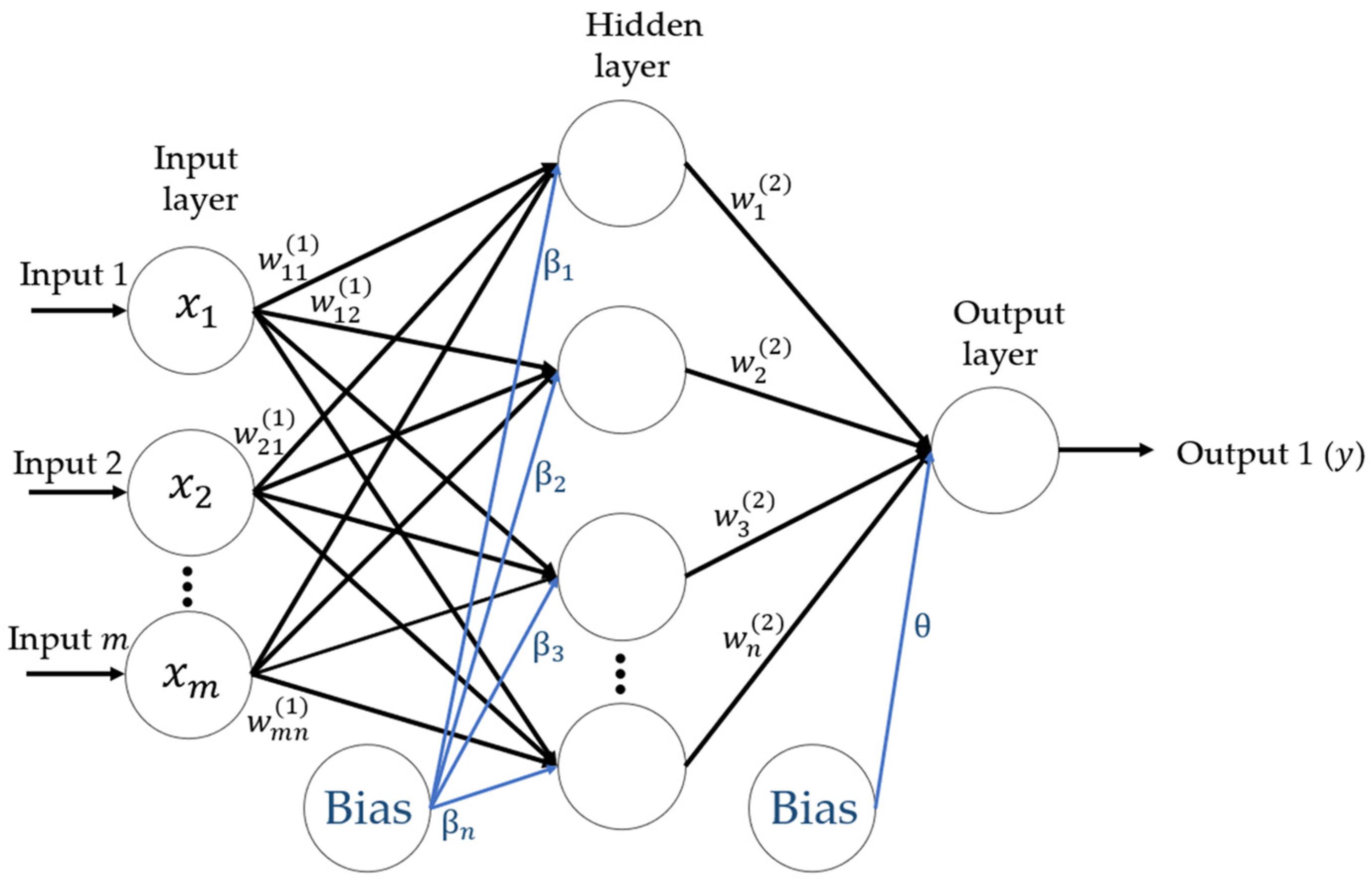
2.2. Artificial Neural Network (ANN)

ANN is a supervised machine learning that has the architecture and function mimicking behavior of neural network in human brain. The structure of ANN imitates the human neural network by connecting artificial neurons together to form a network. This idea was proposed by McCulloch and Pitts in 1943 [30]. ANN is a popular technique for classification and regression problems [31]. One of the most well-known ANN structures is the feed-forward multilayer perceptron model (Figure 1) with the backpropagation algorithm [32]. Typically, a feed-forward multilayer perceptron model has three types of layers such as input layer, hidden layer, and output layer. The artificial neurons in the different layers are joined with synaptic weights. These synaptic weights store the information of the relationship between inputs and outputs.

The input layer contains input nodes. Each input node represents the value from an input feature. The information from the input layer is passed through the first hidden layer. The hidden layers are the layers between the input and output layers. From Figure 1, there is only one hidden layer, but in fact, there can be multiple hidden layers. In general, the greater the number of hidden layers, the more complex relationship that can be stored in the network. The hidden layer consists of hidden nodes receiving information from the previous layer. Then, it aggregates information, transforms the aggregated information with a transfer function, and sends its output, to the next layer. In the output layer, it contains the output nodes that combine and transform the outputs from the last hidden layer into the final outputs. The relationship between inputs ($x_i$) and output ($y$) of the single hidden layer feed-forward ANN is shown as in the below equation:

$$y=\theta +{\displaystyle \sum }_{j=1}^n{w}_j^{\left(2\right)}g\left({\beta }_j+{\displaystyle \sum }_{i=1}^m{w}_{ij}^{\left(1\right)}{x}_i \right)+\epsilon$$

(2)

where $w_j^{\left(2\right)}$ ($j=1,2,\dots ,n$) and $w_{\mathrm{ij}}^{\left(1\right)}$ ($i=1,2,\dots ,m;j=1,2,\dots ,n$) are the weights, ${\theta ,\beta }_j$ are the terms of bias, $\epsilon$ is the white noise, the number of input nodes is $m$, the number of hidden nodes is $n$, and the hidden layer transfer function $g$ is the logistic function [33].

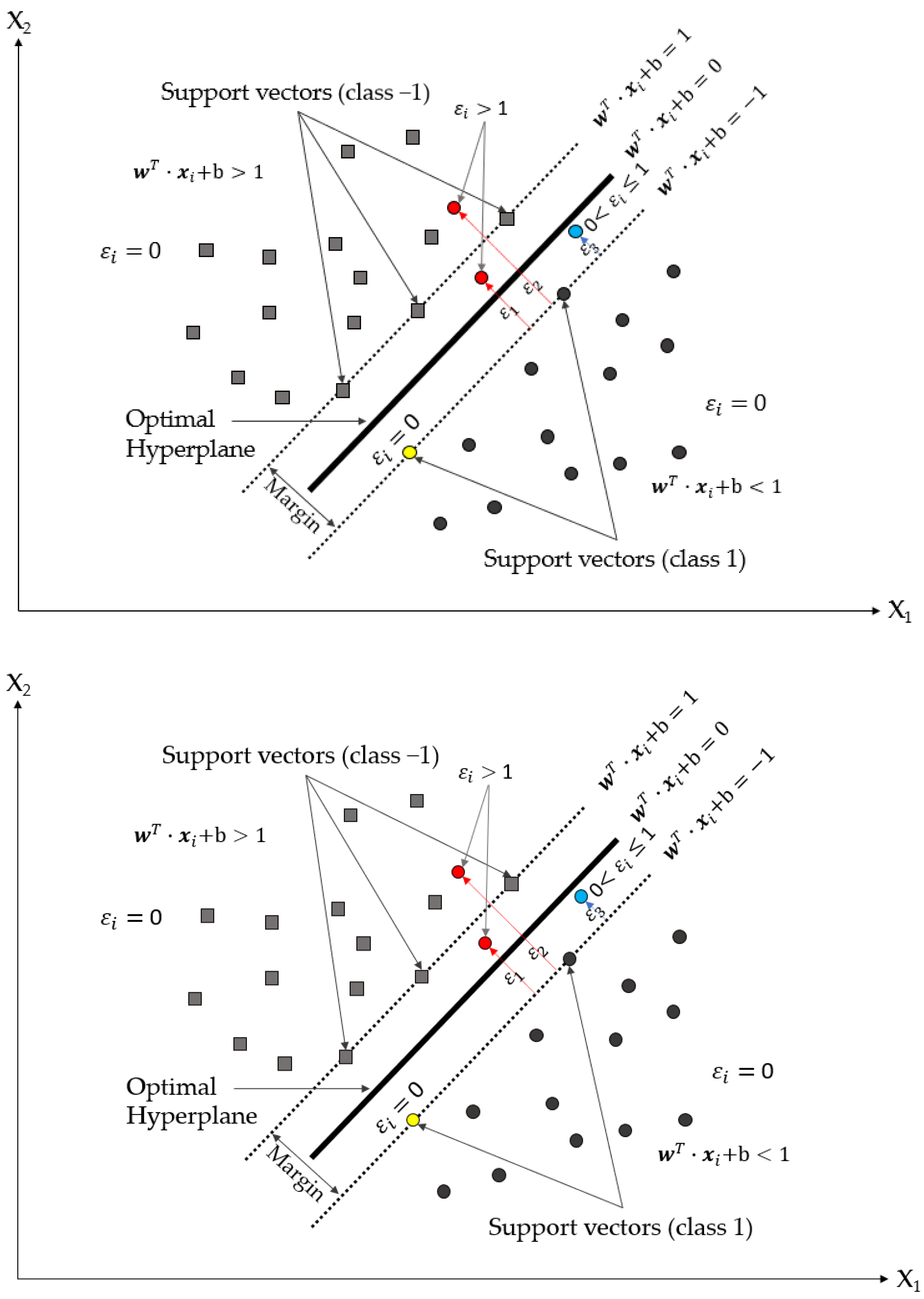
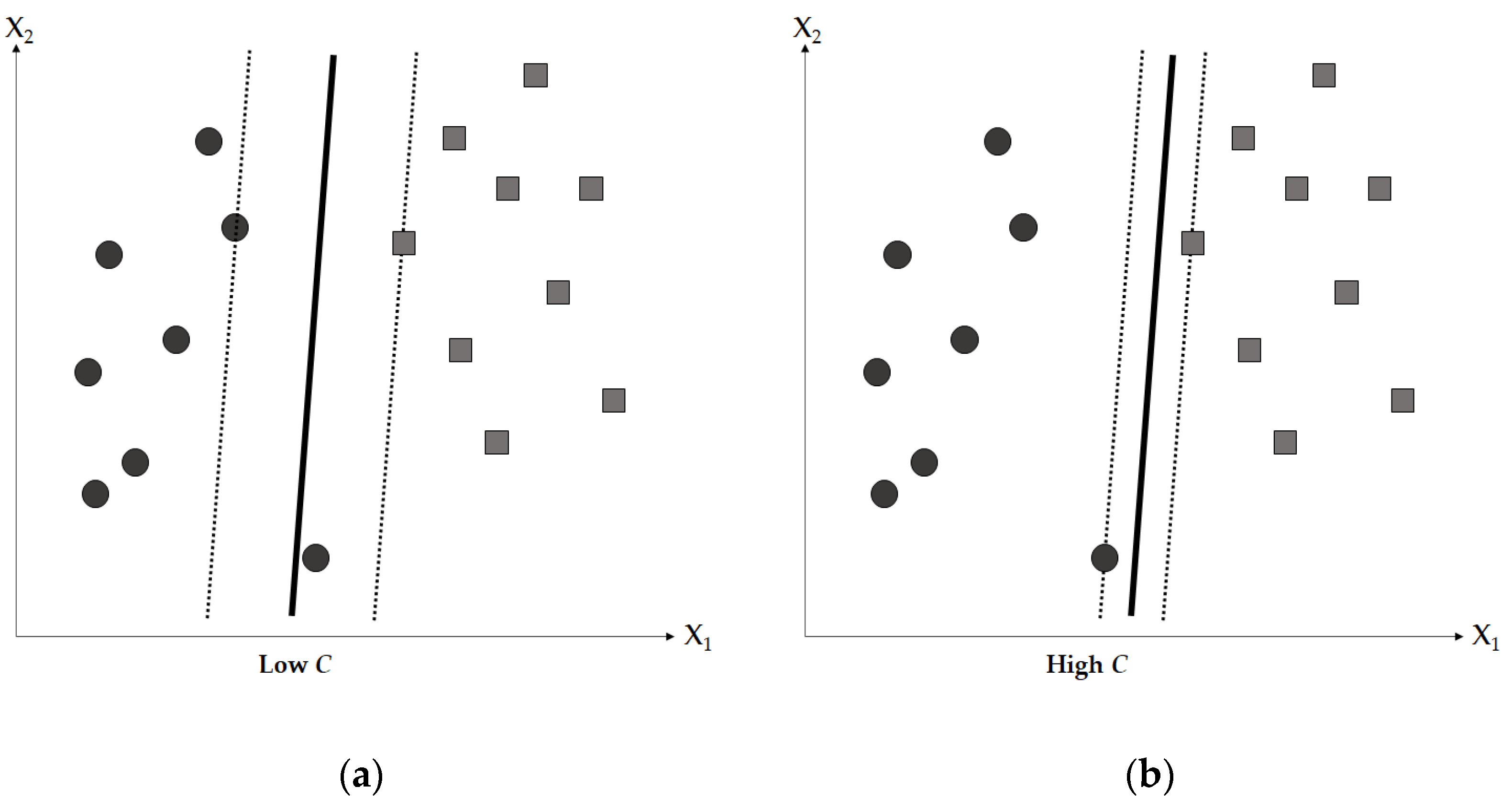
2.3. Support Vector Machine (SVM)

SVM is also a supervised machine learning that can deal with classification and regression problems [34]. Vapnik originally developed SVM [35]. The advantages of SVM are avoiding the overfitting problem as it is good to fit and generalize; performing well for a long-term time series; and using a kernel function to effectively deal with non-linear problems [13]. Theoretically, the objective of SVM is to find an optimal hyperplane which linearly separates the observations into two classes by maximizing the margin. As shown in Figure 2, the solid line is assumed to be the optimal hyperplane. The observations that are nearest to the optimal hyperplane are called support vectors. The boundary is a hyperplane that, is parallel with the optimal hyperplane, and passes the support vectors of a class. The distance between the boundaries is the margin.

In the training process of SVM, the training data can be expressed as $\left(x_1{,y}_1\right){\dots (x}_n{,y}_n)$, where $i$ denotes the number of observations in training data ($n$), $y_i$ denotes class of observation $i$ (i.e., −1 or 1 class), $x_i$ denotes a set of values (real numbers) in D-dimension of observation $i$. In Figure 2, the D-dimension is two. The observations are linearly separable by hyperplanes. To maximize the margin, SVM will solve the optimal value of $w$ and $b$ from the primal optimization problem in Equation (3):

$$\begin{gathered} {\mathrm{Min}}_{{w,b,\epsilon }_i}\left\{\frac{{\Vert w\Vert }^2}{2}+C{\displaystyle \sum }_{i=1}^n{\epsilon }_i\right\}, \\ \mathrm{Subject}\mathrm{to}{y}_i\left(w^T·x_i+b\right)\ge 1-{\epsilon }_i,\forall i\in \left[n\right],\forall y_i\in \{1,-1\}, \\ \mathrm{and}{\epsilon }_i\ge 0,\forall i\in \left[n\right] \end{gathered}$$

(3)

where $w$ denotes a weight vector perpendicular to the optimal hyperplane, $b$ denotes the bias, ${\epsilon }_i$ denotes the positive slack variable of observation $i$, and C is the constant, set by the user.

For ${0<\epsilon }_i\le 1$, the observation $i$ falling within the margin on the correct side of hyperplane is called the margin violation, e.g., the blue circle point in Figure 2. For ${\epsilon }_i>1$, the observation $i$ falling on the wrong side of the separating hyperplane is misclassified, e.g., red circle points in Figure 2. For ${\epsilon }_i=0,$ the observation $i$ is on the correct classification, e.g., yellow circle point in Figure 2. The slack variable can be estimated from Equation (4):

$${\epsilon }_i=\max (0,1-y_i{(w}^T·x_i+b\left)\right)$$

(4)

The constant C defines the trade-off between margin maximization (regularization term) and minimization the misclassified training examples (loss function term). The larger value of C, the narrower margin that has the less misclassification. On the other hand, the smaller value of C, the wider margin that causes the higher misclassification. The different value of C affects the width of margin as shown in Figure 3. Furthermore, to deal with problems where the observations are not linearly separable by the hyperplanes, a kernel method is applied [37].

2.4. Hybrid Models

Referring to the “no free lunch” (NFL theorem), there is no universal algorithm that can perform the best in all circumstances [38]. Applying a hybrid model, a combination of several models, to analyze the problem can reduce the risk of obtaining large prediction errors compared to using only an individual model. The hybrid models can capture the hidden pattern of complex data (e.g., electricity consumption) because they contain unique strengths from multiple individual models.

A widely used hybrid model is linear and non-linear hybrid model [39]. In this paper, Multiple Linear Regression (MLR) is used to capture the linear data behavior. ANN and SVM have the ability to capture non-linear data characteristics. The mathematical relationship between the response variable ($Y_t$) and its components can be computed below:

$$Y_t{=L}_t{+N}_t$$

(5)

where $L_t$ and $N_t$ denote linear and non-linear parts, respectively. In the first step of our proposed hybrid model, the MLR model is used to predict the linear part, i.e., the expected daily consumption. The residuals from the MLR model (${\epsilon }_t$) is expressed below:

$${\epsilon }_t=A_t-{\widehat{L}}_t$$

(6)

where ${\widehat{L}}_t$ and $A_t$ denote the predicted and actual consumption value from MLR model in time period t. Then, the residual (${\epsilon }_t$) from Equation (6) is the non-linear part remaining after extracting the linear part. In the second step, ANN or SVM captures the non-linear part in the residual (${\epsilon }_t$). The predicted non-linear part (${\widehat{N}}_t$) from ANN or SVM model is described below:

$${\widehat{N}}_t=f\left({\epsilon }_{t-1}{,\epsilon }_{t-2}{,\dots ,\epsilon }_{t-n}\right)$$

(7)

where $f$ denotes the function obtained by ANN or SVM. Next, the final prediction value of our proposed hybrid model (${\widehat{Y}}_t$) can be computed as follows:

$${\widehat{Y}}_t{=\widehat{L}}_t{+\widehat{N}}_t$$

(8)

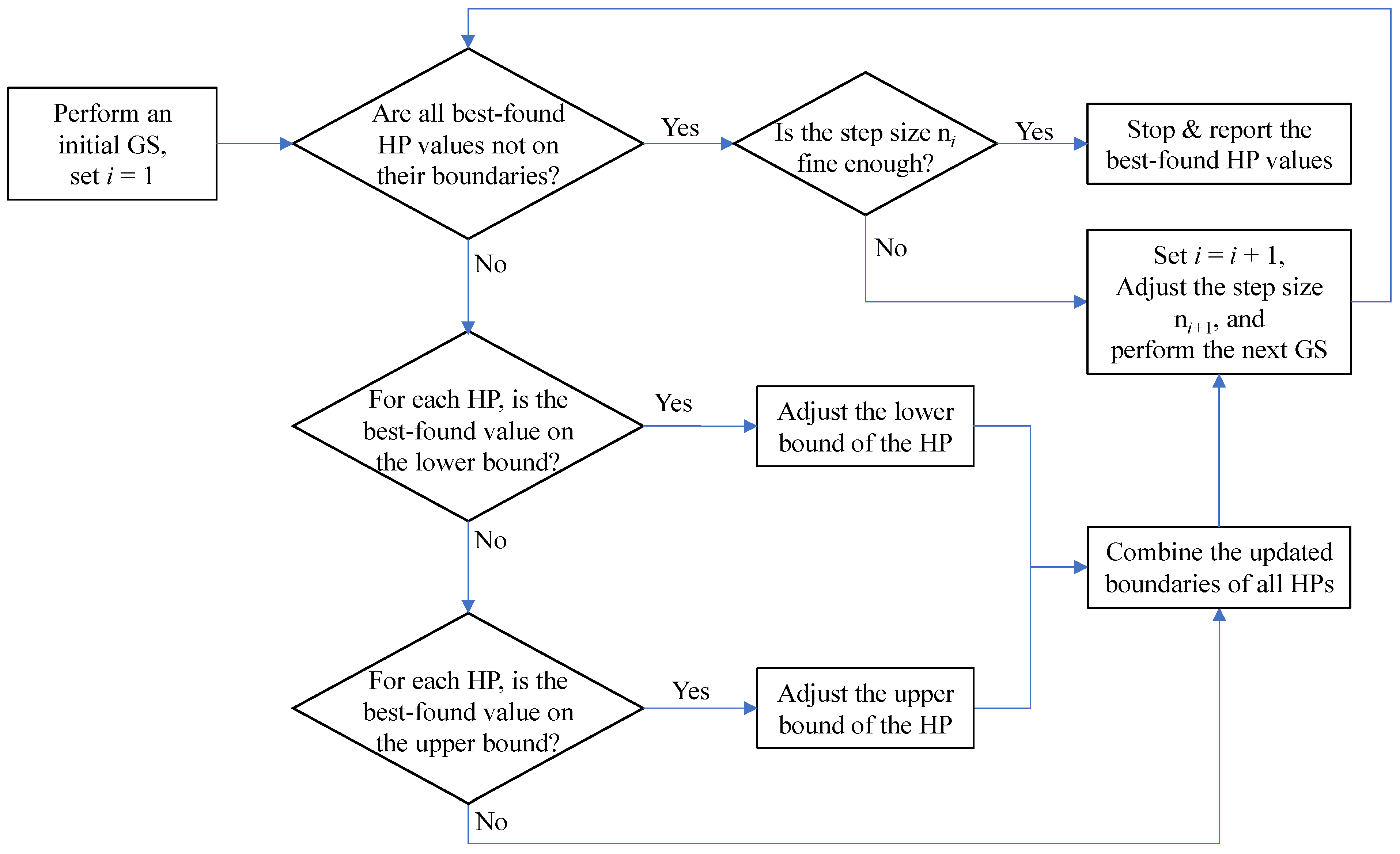
2.5. Sequential Grid Search

Hyperparameter tuning is vital for ML model’s prediction performance. A change of each hyperparameter can make a significant change in model’s accuracy [40]. Grid search is the traditional and simple method for ML hyperparameter tuning [41]. GS completely tests all combinations of hyperparameter values in specified subsets of the hyperparameters. A subset of the hyperparameters can be specified by a lower bound (minimal value), an upper bound (maximal value), and the number of steps [42]. All combinations of hyperparameters are tested to tune ML model in the training process. One drawback is that GS usually requires a large number of runs to properly tune the hyperparameters. In addition, if GS provides a set of best-found hyperparameter values that are on the initial hyperparameter search boundary, then there is a possibility that better hyperparameters are outside of the initial boundary.

To overcome this issue, this article proposes a sequential grid search where search boundaries are adjusted according to whether any of the best-found hyperparameters from a grid search is on the search boundaries. If so, then the boundaries are sequentially adjusted until the best-found values of all hyperparameters are inside the search boundaries. The step of the sequential GS is as shown in Figure 4.

First, initialize the grid search iteration $i$ = 1, specify an initial search boundary, and perform an initial grid search. The initial boundary may be set as a relatively small grid by using a large step size ($n_i$). Then, if all best-found hyperparameter values are not on their search boundaries, then the step size is reduced to make the grid finer, and the subsequent grid search is repeated. However, if at least one of the best-found hyperparameter values is on its boundary, then for each hyperparameter, the sequential grid search checks if the best-found value is on the lower bound, upper bound, or inside the search boundary, so that an adjustment to the boundary is made accordingly. After combining the adjusted search boundaries, the grid search iteration number and the step size are updated to form a new grid, and the next grid search is performed. The sequential grid search repeats until all best-found hyperparameter values are inside the current search boundaries and the step size is small enough. Note that the sequential GS is implemented for the ML model that has multiple hyperparameters, i.e., ANN in this article.

2.6. Forecasting Performance Measurement

Common performance measurements of forecast models are the mean absolute percentage error (MAPE), mean absolute error (MAE), and root mean square error (RMSE). These performance measurements are widely used in electricity consumption forecasting [43]. Their equations are expressed as:

$$\mathrm{MAPE}=\frac{1}{n}{\displaystyle \sum }_{i=1}^n\frac{\left|y_i-{\widehat{y}}_i\right|}{y_i}$$

(9)

$$\mathrm{MAE}=\frac{1}{n}{\displaystyle \sum }_{i=1}^n\left|y_i-{\widehat{y}}_i\right|$$

(10)

$$\mathrm{RMSE}=\sqrt{\frac{1}{n}{\displaystyle \sum }_{i=1}^n\left|y_i-{\widehat{y}}_i\right|}$$

(11)

where $y_i$ is the actual daily electricity consumption in period $i$, ${\widehat{y}}_i$ is the forecast value of daily electricity consumption in period $i$, and $n$ is the total number of periods. In this article, the MAPE is chosen as the main measure of performance since it is used by the industrial user, who provides the data for this study.

Other evaluation metrics used in electricity consumption forecasting are relative prediction error (RPE) [44] and concordance correlation coefficient (CCC) [45]. An RPE higher than 20% indicates that model has poor prediction performance, while a 10–20% of RPE is considered acceptable prediction, and an RPE lower than 10% suggests that the model has satisfactory prediction [46]. A CCC higher than 0.90 indicates that the actual and predicted values have a strong agreement, while 0.80–0.90, 0.65–0.80, and lower than 0.65 of CCC, are considered substantial, moderate, and poor strength of agreement, respectively [47]. RPE and CCC can be computed as follows:

$$\mathrm{RPE}=\frac{\mathrm{RMSE}}{\overline{y}}$$

(12)

$$\mathrm{CCC}=1-\frac{{{(\mu }_1-{\mu }_2)}^2{+(\sigma }_1-{\sigma }_2{)}^2+2(1-{p)\sigma }_1{\sigma }_2}{{\sigma }_1^2{+\sigma }_2^2{+(\mu }_1-{\mu }_2{)}^2}$$

(13)

where $\overline{y}$ is the mean of the actual electricity consumption, $p$ is the Pearson correlation coefficient, ${\mu }_1$ is the mean actual electricity consumption, ${\mu }_2$ is the mean of the predicted daily electricity consumption, ${\sigma }_1$ is the standard deviation of the actual electricity consumption, ${\sigma }_2$ is the standard deviation of the predicted electricity consumption, ${\sigma }_1^2$ is the variance of the actual electricity consumption, and ${\sigma }_2^2$ is the variance of the predicted electricity consumption.

3. Computational Experiment

3.1. Data Partitioning

The historical data of daily electricity consumption from 2009 to 2018, a total of 3652 observations, are divided into three datasets: training, validation, and test. The data partitioning is performed using chronological order of the data due to its time-series nature. The training set contains observations from 2009 to 2016, while the 2017 data are for validation purpose, and the 2018 data are the test set.

3.2. Input Attributes

The electricity consumption data are illustrated in Figure 5. The graph shows not only an increasing trend, but also a seasonal (yearly) pattern. Hence, moving average (MA) and seasonal index (SI) variables were created as input attributes. Moreover, electricity consumption tends to increase from 2009 to 2015, and then become relatively more stable from 2016 to 2018.

Five moving average MA(L) variables, including MA(7), MA(30), MA(90), MA(120), and MA(365), are created. MA(7) is a weekly moving average with a span of seven days. Similarly, MA(30), MA(90), MA(120), and MA(365) are monthly, quarterly, seasonally (Thailand has three seasons, each of which spans approximately four months), and yearly moving averages, respectively. Seasonal index (SI) variables are estimated for each month in each year. MA and SI are computed using Equations (14) and (15):

$$\mathrm{MA}\left(L\right)=\frac{y_{t-1}{+y}_{t-2}{+\dots +y}_{t-L}}{L}$$

(14)

$${\mathrm{SI}}_{ij}=\frac{{{\displaystyle \sum }}_{t\in \{i,j\}}{y}_t}{{{\displaystyle \sum }}_{t\in \left\{j\right\}}{y}_t}$$

(15)

where $y_t$ denotes the daily electricity consumption in day $t$ ∈ {1, 2, …, 3652}, $L$ is the length of MA, $i$ represents the month index from January to December, and $j$ is the year index from 2009 to 2018. For example, ${\mathrm{SI}}_{Jan,2009}$ is computed from the total electricity consumption in January 2009, divided by the total electricity consumption in 2009.

To improve the forecast performance of the ML models, additional input attributes are created. First, the lagged daily consumption variables are created with the lags of 1, 2, …, 7, 30, 60, 90, and 365 days, e.g., a one-day lagged variable is y_t−1. In other words, lagged variables of one to seven days, a month, two months, a quarter, and one year are created. Another created variable is a seven-day-ago peak of electricity consumption. This variable is the maximum consumption within a day that occurred seven days ago.

In addition, some fundamental variables are used in the ML prediction models. These variables include the previous day’s highest temperature reported by the Meteorological Department of Thailand, and indicator variables representing national holiday, bridging holiday, weekend, month of the year, and day of the week (Monday to Sunday). It should be noted that the MLR model only includes the highest temperature variable, but without other meteorological variables, e.g., rainfall, humidity, solar radiation, for two reasons. First, it is due to the availability of the data that the industrial user has access to. Second, because the forecast is made for the whole country, some meteorological variables that are more local in terms of geography, such as rainfall, humidity, etc., are not included, since there are hundreds of weather stations throughout Thailand. On the other hand, the variable, i.e., temperature, that may well represent the weather condition of the whole country is included. Based on the initial analysis of temperature data, the user only chooses to include the average peak temperature since it may significantly affect the amount of air conditioning usage. As a substitute to other meteorological variables, the model contains indicator variables for different months, which, in a sense, represent different meteorological data at different time of a year.

Regarding national holidays, there are two types of national holidays in Thailand. One type is a national holiday that is specific to a date on the calendar, e.g., New Year’s Day or Father’s Day, and the other type is a non-specific date that changes every year, e.g., Buddhist Lent Day or Chinese New Year. Moreover, a bridging holiday is an additional holiday announced by the government, which usually is the day that bridges a weekend with a national holiday.

3.3. MLR Model Result

First, the MLR model is fitted with all input variables as an initial model. The total number of variables is 41, which are: the seven-day-ago peak of electricity consumption, highest temperature of the previous day, 11 different lagged variables of past daily consumption, five moving average variables, a seasonal index, 3 indicator variables for being a national holiday, bridging holiday, or weekend, 12 indicator variables for months of the year, and 7 indicator variables for days of the week. Then, we use a model fitting technique, called stepwise regression, to obtain the final MLR model. The stepwise regression alternately adds important variables to the model and eliminates unimportant variables from the model using two criteria: significance level for a variable to be included in the model ($\alpha$-to-enter) and a significance level for a variable to be eliminated from the model ($\alpha$-to-remove). The final MLR model that best fits with the training data is obtained from the stepwise regression with α-to-enter and α-to-remove equal to 0.1. The final regression model containing only 24 important variables is given in Equation (16) below:

$$\begin{gathered} \widehat{y}=8069+1{.008x}_1{+2048x}_2+0{.8455x}_3-0{.2350x}_4+0{.0538x}_5 \\ -0{.0239x}_6-0{.0378x}_7+0{.1589x}_8+0{.1505x}_9-{51069x}_{10}-{34471x}_{11} \\ -{23059x}_{12}-{8781x}_{13}-{4137x}_{14}{+2064x}_{15}{+6142x}_{16}-{2090x}_{17} \\ {+2617x}_{18}-{2677x}_{19}-{9205x}_{20}{+41297x}_{21}{+6502x}_{22}-{4711x}_{23}-{38531x}_{24}+ϵ \end{gathered}$$

(16)

where $\widehat{y}$ is the forecast of daily electricity consumption, $x_1$ is 7-day-ago peak of daily electricity consumption, $x_2$ is the previous day’s highest temperature, $x_3$ to $x_8$ are 1-day, 2-day, 3-day, 4-day, 5-day, and 365-day lagged consumption variables, $x_9$ is MA(30), $x_{10}$ is seasonal index of the same month in the previous year, $x_{11}$ to $x_{24}$ are indicator variables for national holiday, bridging holiday, weekend, February, March, May, June, August, November, December, Monday, Tuesday, Friday, and Sunday, respectively. It can be seen from the final model that that the important variables that can be used to effectively forecast the daily consumption are (1) the 30-min peak of consumption from 7 days ago and the highest temperature of the previous day, (2) the lagged daily consumption variables from 1, 2, 3, 4, and 5 days ago, as well as 365 days ago (same date of the previous year), (3) the moving average of the previous 30-day, (4) seasonal index, (5) being a national holiday, bridging holiday, or weekend, (6) 7 out of 12 months have significant different daily consumptions than the other 5 months, and (6) being Tuesday (highest daily consumption on average), Friday (lowest daily consumption among weekdays), and Sunday (lowest daily consumption of the week).

The final MLR model is then used to forecast daily electricity consumption of the validation set and test set. The analysis of variance of the MLR model and the MAPE for each dataset are shown in

Table 1. Analysis of variance of MLR.

Source	DF	Adj SS	Adj MS	F-Value	p-Value
Regression	24	6.73 × 1012	2.80 × 1011	1774.48	0.000
Error	2532	4.00 × 1011	1.57 × 108
Total	2556	7.13 × 1012

Note: DF denotes the degree of freedom of each source of variability, Adj SS is the adjusted sums of squares, and Adj MS is adjusted mean squares.

and

Table 2. MAPE of MLR.

Dataset	Train	Validation	Test
MAPE (%)	1.9234	2.1977	2.0225

, respectively.

3.4. Hyperparameter Tuning of ML Models Using Sequential Grid Search

3.4.1. Sequential Grid Search for Hyperparameter Tuning of ANN

An ANN model is initially constructed using the training dataset. The hyperparameter (HP) values of ANN, including training cycles (TC), learning rate (LR), and momentum rate (MR), are chosen based on the prediction performance of the validation dataset. After tuning the HPs, the ANN model is then evaluated with the unseen data of the test set. In addition, the architecture of the ANN is also varied from 1 to 15 hidden nodes in one hidden layer.

The sequential grid search is initialized with the number of neurons (or nodes) in the hidden layer, denoted as HN, set to one. The first grid search is performed according to the three HP ranges, the number of steps, and values as shown in

Table 3. First grid search for ANN hyperparameters.

Hyperparameter	Min	Max	Step	Values
TC	100	1000	5	100, 280, 460, …, 1000
LR	0.001	0.05	5	0.001, 0.0108, 0.0206, …, 0.05
MR	0.5	0.9	5	0.5, 0.58, 0.66, …, 0.9

. The activation function for ANN is the sigmoid function, which is widely used in a number of research studies [48,49,50,51]. The convergence epsilon is set at 0.0001. All combinations of the three HPs are generated, where each HP is varied according to the number of steps (i.e., five times) from the lower bound to the upper bound. This results in a total of 216 combinations for the initial grid search.

The results of the initial grid search are analyzed using the procedure in Figure 4. The analysis result leads to the hyperparameter setting of the subsequent grid search, where the minimum, maximum, and number of steps depend on the results of the previous grid search.

Table 4. Values of ANN hyperparameters in the sequential grid search.

Hyperparameter	Min	Max	Step	Values
TC	100	1000	10	100, 190, 280, …, 1000
	100	1000	20	100, 145, 190, …, 1000
	550	1450	10	550, 640, 730, …, 1450
	550	1450	20	550, 595, 640, …, 1450
	10	910	10	10, 100, 190, …, 910
	10	910	20	10, 55, 100, …, 910
	1000	1900	20	1000, 1045, 1090, …, 1900
LR	0.001	0.05	10	0.001, 0.0059, 0.0108, …, 0.05
	0.001	0.05	20	0.001, 0.00345, 0.0059, …, 0.05
	0.0001	0.0491	10	0.0001, 0.005, 0.0099, …, 0.0491
	0.0001	0.0491	20	0.0001, 0.00255, 0.005, …, 0.0491
	0.0255	0.0745	10	0.0245, 0.0295, 0.0345, …, 0.0745
	0.0255	0.0745	20	0.0245, 0.027, 0.0295, …, 0.0745
MR	0.5	0.9	10	0.5, 0.54, 0.58, …, 0.9
	0.5	0.9	20	0.5, 0.52, 0.54, …, 0.9
	0.6	1	10	0.6, 0.64, 0.68, …, 1
	0.6	1	20	0.6, 0.62, 0.64, …, 1
	0.3	0.7	10	0.3, 0.34, 0.38, …, 0.7
	0.3	0.7	20	0.3, 0.32, 0.34, …, 0.7

shows the ranges and values of each hyperparameter used in the sequential grid search of ANN.

After completing the subsequent grid search for the ANN with HN equal to 1, HN is increased by 1, and the sequential grid search procedure is repeated until HN reaches 15 nodes. The results from performing the sequential grid search for each HN are reported in

Table 5. Sequential grid search result of ANN (Hyperparameter values in bold indicate the values are on the search boundaries).

HN	GS Step	TC			LR			MR			Best Found HP			MAPE
		Min	Max	Step	Min	Max	Step	Min	Max	Step	TC	LR	MR	Train	Validate	Test
1	1	100	1000	5	0.001	0.05	5	0.5	0.9	5	280	0.001	0.90	1.98	2.20	2.03
	2	100	1000	10	0.0001	0.0491	10	0.6	1	10	640	0.00990	0.60	2.02	2.18	2.07
	3	100	1000	20	0.0001	0.0491	20	0.3	0.7	20	190	0.0148	0.50	2.02	2.16	2.07
2	1	100	1000	5	0.001	0.05	5	0.5	0.9	5	280	0.01080	0.58	1.83	1.99	1.91
	2	100	1000	20	0.001	0.05	20	0.5	0.9	20	730	0.00835	0.88	1.81	1.96	1.84
3	1	100	1000	5	0.001	0.05	5	0.5	0.9	5	640	0.03040	0.66	1.80	1.93	1.90
	2	100	1000	20	0.001	0.05	20	0.5	0.9	20	955	0.04755	0.62	1.71	1.89	1.82
4	1	100	1000	5	0.001	0.05	5	0.5	0.9	5	820	0.02060	0.58	1.73	1.92	1.89
	2	100	1000	20	0.001	0.05	20	0.5	0.9	20	775	0.00835	0.68	1.70	1.89	1.76
5	1	100	1000	5	0.001	0.05	5	0.5	0.9	5	1000	0.01080	0.82	1.57	1.90	1.80
	2	550	1450	10	0.001	0.05	10	0.5	0.9	10	1360	0.03040	0.62	1.52	1.85	2.03
	3	550	1450	20	0.001	0.05	20	0.5	0.9	20	730	0.02305	0.70	1.57	1.86	1.96
6	1	100	1000	5	0.001	0.05	5	0.5	0.9	5	1000	0.02060	0.74	1.49	1.94	1.84
	2	550	1450	10	0.001	0.05	10	0.5	0.9	10	1270	0.01570	0.82	1.49	1.89	1.79
	3	550	1450	20	0.001	0.05	20	0.5	0.9	20	1225	0.02795	0.68	1.52	1.86	1.84
7	1	100	1000	5	0.001	0.05	5	0.5	0.9	5	820	0.04020	0.66	1.52	1.90	1.74
	2	100	1000	20	0.001	0.05	20	0.5	0.9	20	595	0.03530	0.90	1.49	1.86	1.82
	3	100	1000	20	0.001	0.05	20	0.6	1	20	1000	0.02060	0.80	1.57	1.88	1.68
	4	550	1450	20	0.001	0.05	20	0.6	1	20	1450	0.02060	0.80	1.54	1.86	1.68
	5	1000	1900	20	0.001	0.05	20	0.6	1	20	1855	0.00345	0.94	1.49	1.85	1.69
8	1	100	1000	5	0.001	0.05	5	0.5	0.9	5	640	0.02060	0.66	1.58	1.96	1.94
	2	100	1000	20	0.001	0.05	20	0.5	0.9	20	865	0.02795	0.68	1.51	1.89	2.07
9	1	100	1000	5	0.001	0.05	5	0.5	0.9	5	1000	0.01080	0.90	1.44	1.95	2.40
	2	550	1450	10	0.001	0.05	10	0.6	1	10	1450	0.0206	0.68	1.46	1.91	2.11
	3	550	1450	20	0.001	0.05	20	0.6	1	20	1360	0.04755	0.66	1.4	1.87	2.02
10	1	100	1000	5	0.001	0.05	5	0.5	0.9	5	460	0.05	0.66	1.53	1.97	2.09
	2	100	1000	10	0.0255	0.0745	10	0.5	0.9	10	910	0.04950	0.78	1.49	1.93	2.23
	3	100	1000	20	0.0255	0.0745	20	0.5	0.9	20	865	0.02700	0.68	1.45	1.93	2.07
11	1	100	1000	5	0.001	0.05	5	0.5	0.9	5	100	0.03040	0.66	1.72	2.00	1.97
	2	10	910	10	0.001	0.05	10	0.5	0.9	10	640	0.03530	0.66	1.52	1.96	1.92
	3	10	910	20	0.001	0.05	20	0.5	0.9	20	775	0.04755	0.66	1.50	1.92	1.99
12	1	100	1000	5	0.001	0.05	5	0.5	0.9	5	1000	0.02060	0.58	1.49	1.93	1.88
	2	550	1450	10	0.001	0.05	10	0.5	0.9	10	1360	0.02060	0.50	1.45	1.93	1.89
	3	550	1450	10	0.001	0.05	10	0.3	0.7	10	1270	0.03040	0.50	1.47	1.94	1.88
	4	550	1450	20	0.001	0.05	20	0.3	0.7	20	1405	0.02795	0.32	1.46	1.88	1.89
13	1	100	1000	5	0.001	0.05	5	0.5	0.9	5	820	0.03040	0.66	1.42	1.98	2.15
	2	100	1000	20	0.001	0.05	20	0.5	0.9	20	685	0.02305	0.58	1.52	1.91	2.12
14	1	100	1000	5	0.001	0.05	5	0.5	0.9	5	820	0.02060	0.66	1.48	1.98	2.07
	2	100	1000	20	0.001	0.05	20	0.5	0.9	20	1000	0.04020	0.58	1.43	1.93	2.38
	3	550	1450	20	0.001	0.05	20	0.5	0.9	20	685	0.03775	0.54	1.47	1.93	2.10
15	1	100	1000	5	0.001	0.05	5	0.5	0.9	5	640	0.03040	0.66	1.53	1.97	1.99
	2	100	1000	20	0.001	0.05	20	0.5	0.9	20	910	0.02305	0.74	1.40	1.96	2.19

. Each row contains the setting of one grid search, which includes the boundary and number of steps of TC, LR, and MR, as well as the best-found values of HPs from the grid search, along with the prediction performance (MAPE) on the train, validation, and test sets. For example, the first row indicates that after testing 6 × 6 × 6 = 216 sets of HPs for ANN with one node in the hidden layer, the best-found HPs among 216 ANNs are TC = 280, LR = 0.001, and MR = 0.9, which results in MAPE of 1.98%, 2.20%, and 2.03% for the train, validate, and test sets, respectively.

According to the procedure in Figure 5, the best value of TC from the first grid search does not fall on its boundary, so the search boundary of LR remains unchanged for the next grid search (in the second row). However, the best LR falls at the minimum value of its search boundary, and the best MR falls at the maximum value of its search boundary. Therefore, the minimum value of LR becomes the middle of the search boundary for the next grid search. Similarly, the maximum value of MR becomes the middle of the search boundary of the next grid search. Additionally, the number of steps is set to 10 for the second grid search (2nd row). Based on the boundary and number of steps, the 2nd grid search contains 11 × 11 × 11 = 1331 sets of HPs (i.e., 1331 ANN tested). From the 2nd grid search, the best-found HPs are TC = 640, LR = 0.0099, and MR = 0.60, and MAPE for the train, validate, and test of 2.02%, 2.18%, and 2.07%, respectively.

The sequential grid search is repeated until either the best-found HPs do not fall on the search boundaries of all HP or the number of steps reaches 20. After performing all sequential grid search for HN from 1 to 15, the total number of ANNs tested in Table 5 is 189,847 models.

One factor that defines the architecture of ANN is the number of nodes in the hidden layer, called “model size” in this paper. From the sequential grid search results, the best five settings of ANN among all model sizes and the best five settings of ANN for each model size are listed in

Table 6. Best five settings of ANN of all model sizes and of each model size from sequential grid search.

All Model Sizes				MAPE (%)			Each Model Size				MAPE (%)
HN	TC	LR	MR	Train	Val.	Test	HN	TC	LR	MR	Train	Val.	Test
5	1360	0.03040	0.62	1.5161	1.8500	2.0299	5	1360	0.03040	0.62	1.5161	1.8500	2.0299
6	1225	0.02795	0.68	1.5221	1.8576	1.8358	6	1225	0.02795	0.68	1.5221	1.8576	1.8358
7	595	0.03530	0.90	1.4862	1.8563	1.8163	7	1855	0.00345	0.94	1.4853	1.8545	1.6889
5	730	0.02305	0.70	1.5687	1.8648	1.9583	9	1360	0.04755	0.66	1.3977	1.8704	2.0244
7	1855	0.00345	0.94	1.4853	1.8545	1.6889	12	1405	0.02795	0.32	1.4642	1.8754	1.8925

. Note that the model size is characterized by HN (or the number of neurons in the hidden layer) and that these settings are selected based on the validation set MAPE.

3.4.2. Grid Search for Hyperparameter Tuning of SVM

The training and the validation datasets are used to train and tune the hyperparameter of SVM, respectively. The SVN is constructed with a convergence epsilon of 0.001. Three kernel functions, including dot, radial, and polynomial are tested. SVM hyperparameters that are considered are C, gamma, and polynomial degree. The hyperparameters for each kernel function are shown in

Table 7. Hyperparameters for each kernel function.

Kernel Fuctions	Hyperparameter Adjusting	The Number of Runs
dot	C	40
radial	C, GAMMA	626
polynomial	C, polynomial degree	200

.

In the grid search, C, gamma, and polynomial degree are varied according to the ranges in

Table 8. Values of SVM hyperparameters in the grid search.

Hyperparameter	Min	Max	Step	Scale	Values
C and Gamma	0.0001	1000	7	Exponential	0.0001, 0.001, 0.01, …, 1000
	$2^{-10}$	$2^{10}$	20	Exponential	$2^{-10}{,2}^{-9}{,2}^{-8}{,\dots ,2}^{10}$
	0.0001	1000	10	Logarithmic	0.0001, 0.9956, 2.9820, …, 1000
Polynomial Degree	1	5	4	Linear	1, 2, 3, …, 5

, from the minimum to the maximum values with the specified number of steps. Note that C and gamma are tested in three separate ranges (rows 1–3 of Table 8), while polynomial degree is tested in one range (row 4). For example, in the first row of Table 8, C is changed from 0.0001 to 1000 in seven steps on an exponential scale, resulting in eight values. For dot kernel function, only C is tested, therefore, the grid search contains (8 + 21 + 11) runs from the three parameter ranges combined. For radial kernel function, both C and gamma are varied together within each of the three ranges in the grid search. That is a total of (8² + 21² + 11²) = 626 runs. For polynomial degree, the grid search contains (8 + 21 + 11) × 5 = 200 runs. In total, the grid search contains 866 runs. After performing all grid searches, the five settings that have the lowest MAPE of the validation set are from the polynomial kernel function with the hyperparameter values as shown in

Table 9. Best five settings of SVM from grid search.

			Polynomial	MAPE (%)
Setting	Kernel Function	C	Degree	Train	Validate	Test
1	polynomial	64	2	1.4617	2.2039	2.0792
2	polynomial	62.1337	2	1.4656	2.2049	2.0841
3	polynomial	512	1	1.9082	2.2087	2.0613
4	polynomial	500.6383	1	1.9108	2.2091	2.0650
5	polynomial	1000	1	1.9160	2.2118	2.0414

.

3.4.3. Sequential Grid Search for Hyperparameter Tuning of Hybrid of MLR and ANN and Hybrid of MLR and SVM

In the hybrid models, the residuals from the final MLR model in Equation (16) are used as the response variables for prediction by another ANN model and SVM model. The same sequential grid search for hyperparameter tuning of ANN are performed in the same manner as the ones in Section 3.4.1 and 3.4.2, respectively. The best five settings of ANN of all model sizes (denoted hybrid model 1, or HM 1), the best five settings of ANN of each model size (HM 2), and the best five SVMs (HM 3) from Table 6 and Table 8 are used to predict the values of the residuals. Forecast values of HM 1 are from adding the average predicted residuals (from the five settings of ANN) to the predicted electricity consumption from the final MLR model. An example of using HM 1 to create the forecast values of the test set is given in

Table 10. Hybrid model of MLR and five best ANN of all model sizes.

Date $t$	${\widehat{L}}_t$ from MLR	${\widehat{N}}_t$ from Five Best ANN of Each Model Size					Avg. ${\widehat{N}}_t$	${\widehat{Y}}_t$	Absolute % Error
		5-Node	6-Node	7-Node	5-Node	7-Node
1 January 2018	350,672.94	−40,798.68	−24,283.33	−32,441.42	−37,417.81	−25,044.95	−31,997.24	318,675.70	6.87%
2 January 2018	305,652.51	−13,009.44	−10,922.76	−2008.96	−10,722.67	43,120.87	1291.41	306,943.92	4.25%
⋮	⋮	⋮	⋮	⋮	⋮	⋮	⋮	⋮	⋮
30 December 2018	349,037.20	−3196.13	−825.11	−1239.31	5450.93	−3816.26	−725.18	348,312.02	0.03%
31 December 2018	366,322.07	−82,552.53	−108,228.36	−14,142.70	−59,456.21	−54,299.94	−63,735.95	302,586.12	3.20%
								MAPE	1.78%

Note: ${\widehat{L}}_t$ = predicted consumption, ${\widehat{N}}_t$ = predicted residual, ${\widehat{Y}}_t$ = final forecast, ${\widehat{L}}_t+{\widehat{N}}_t$.

. The MAPE of the test set from HM 1 is 1.78%. Similarly, examples of forecast values of HM 2 and HM 3 are given in

Table 11. Hybrid model of MLR and five best ANN of each model size.

Date $t$	${\widehat{L}}_t$ from MLR	${\widehat{N}}_t$ from Five Best ANN of Each Model Size					Avg. ${\widehat{N}}_t$	${\widehat{Y}}_t$	Absolute % Error
		5-Node	6-Node	7-Node	5-Node	7-Node
1 January 2018	350,672.94	−40,798.68	−24,283.33	−25,044.95	−25,007.89	−19,471.74	−26,921.32	323,751.62	8.57%
2 January 2018	305,652.51	−13,009.44	−10,922.76	43,120.87	34,046.03	19,380.34	14,523.01	320,175.52	0.12%
⋮	⋮	⋮	⋮	⋮	⋮	⋮	⋮	⋮	⋮
30 December 2018	349,037.20	−3196.13	−825.11	−3816.26	−16,416.08	1442.55	−4562.21	344,474.99	1.13%
31 December 2018	366,322.07	−82,552.53	−108,228.36	−54,299.94	−69,009.25	−78,190.98	−78,456.21	287,865.86	7.91%
								MAPE	1.76%

and

Table 12. Hybrid model of MLR and five best SVM.

Date $t$	${\widehat{L}}_t$ from MLR	${\widehat{N}}_t$ from Five Best ANN of Each Model Size					Avg. ${\widehat{N}}_t$	${\widehat{Y}}_t$	Absolute % Error
		SVM 1	SVM 2	SVM 3	SVM 4	SVM 5
1 January 2018	350,672.94	−18,048.38	−19,562.62	7877.70	5124.41	4303.32	−4061.11	346,611.83	16.24
2 January 2018	305,652.51	−15,599.19	−16,813.18	−2992.27	−6944.18	−8333.85	−10,136.53	295,515.98	7.81
⋮	⋮	⋮	⋮	⋮	⋮	⋮	⋮	⋮	⋮
30 December 2018	349,037.20	−7380.02	−7096.51	−6027.58	−7548.98	−8079.29	−7226.48	341,810.72	1.90
31 December 2018	366,322.07	−31,846.23	−30,554.54	8238.38	6865.69	6330.87	−8193.17	358,128.90	14.57
								MAPE	1.83%

. MAPE of the two hybrid models are 1.76% and 1.83%, respectively. It can be seen that the performance of HM 1 and HM 2 are superior to that of HM 3. In other words, the hybrid models of MLR and ANN perform better than the hybrid model of MLR and SVM.

3.5. Ensemble Prediction Models

Ensemble model is a type of model that combines forecast values from multiple models to create the final forecast values. In this paper, the combined forecast values are simply the average forecast values of the multiple models. To build an ensemble model, a number of forecasting models are selected by using the minimal MAPE on the validation set. The performance of the ensemble models is evaluated on unseen data of the test set. In this paper, MAPE is used as the main criteria to compare ensemble models.

Two ensemble ANN models, EM 1 and EM2, are built from the best five ANN of all model sizes and of each model size in Table 5. Similarly, EM 3 is an ensemble SVM model containing the best five SVM models from the grid searches in Table 6. MAPE of the test set from the three ensembled models are 1.6827%, 1.7373%, and 1.9345%, respectively. Based on the result, the ensemble model containing the best five ANN of all model sizes performs better than other ensemble models.

3.6. Adding Indicator Variables for Each Specific National Holiday to Improve Performance

To illustrate the model performance, Figure 6 illustrates the actual electricity consumption and its forecast value from the best ensemble model EM 1 of the test set, along with the absolute value of forecast error (see the error scale on the right vertical axis).

Data points with large errors in which EM 1′s forecast values significantly over-estimate or under-estimate the actual data can be noticed from Figure 6 These are data points that are related to holidays or bridging holidays in a year. Some are holidays with fixed dates on the standard calendar, while others are the holidays whose dates change every year since they are related to the lunar calendar. The fixed date holidays with large forecast errors include New Year’s Day, Labor Day (1 May in Thailand), Chakri Memorial Day (6 April), Songkran festival (13–15 April) Vajiralongkorn Day (29 July), Mother’s Day (12 August), Chulalongkorn Day (23 October), Father’s Day (5 December), and Constitutional Day (10 December). Moving date holidays are related to Buddhism, including Fourfold Assembly Day, Buddha Day, and Asalha Puja Day.

Plotting similar graphs for the training and validation sets reveals that large errors can be observed on these dates in each year. Therefore, an adjustment to further improve the model performance is to add some indicator (binary) variables for these dates in a year as part of the input data. It is important to emphasize that each of the additional indicator variables proposed here are tied to a specific national holiday, either fixed date or moving date. This is different from using one binary variable to indicate whether a date is a national holiday. This is because the effects of different national holidays are not the same. The MAPE of the test set from various models are used to evaluate the impact of adding indicator variables. These models include the final MLR model, the best ANN and SVM obtained from sequential grid search, the three hybrid models (HM 1–HM 3), and the three ensemble models (EM 1–EM 3). The results are presented in

Table 13. Impact of adding indicator variables on various forecast performance.

Model	MAPE (%) of Test Set			MAE (Mwh) of Test Set			RMSE (MWh) of Test Set			RPE (%) of Test Set			CCC of Test Set
	Indicator Var.		Imp. (%)	Indicator Var.		Imp. (%)	Indicator Var.		Imp. (%)	Indicator Var.		Imp. (%)	Indicator Var.		Imp. (%)
	w/o	with		w/o	with		w/o	with		w/o	with		w/o	with
MLR	2.0225	1.951	0.07	10,095.08	9803.35	2.89	13,903.14	13,282.35	4.47	2.67%	2.55%	0.0012	0.9479	0.9526	0.5
ANN	2.0299	1.7022	0.33	10,361.65	8602.6	16.98	13,365.53	11,787.23	11.81	2.57%	2.26%	0.0031	0.9566	0.9644	0.82
SVM	2.0792	2.0883	−0.01	10,552.66	10,644.35	−0.87	13,511.58	14,654.99	−8.46	2.59%	2.81%	−0.0022	0.9526	0.9471	−0.58
HM 1	1.7814	1.5664	0.22	9079.72	7962.4	12.31	12,448.35	10,819.90	13.08	2.39%	2.08%	0.0031	0.9609	0.971	1.05
HM 2	1.7556	1.5801	0.18	8931.22	8030.73	10.08	12,378.63	11,096.21	10.36	2.38%	2.13%	0.0025	0.961	0.969	0.83
HM 3	1.8263	1.6982	0.13	9131.19	8491.27	7.01	12,756.5	12,148.24	4.77	2.45%	2.33%	0.0012	0.9573	0.9618	0.47
EM 1	1.6827	1.572	0.11	8591.81	7927.51	7.73	11,654.92	11,405.80	2.14	2.24%	2.19%	0.0005	0.9657	0.9679	0.23
EM 2	1.7373	1.7149	0.02	8875.55	8659.77	2.43	11,870.89	12,072.37	−1.70	2.28%	2.32%	−0.0004	0.9656	0.9643	−0.13
EM 3	1.9345	1.8395	0.1	9679.2	9311.78	3.8	13,114.17	12,522.50	4.51	2.52%	2.40%	0.0012	0.9541	0.9592	0.53

.

Based on MAPE, eight out of nine models, except SVM, have achieved some improvement. The best model after adding indicator variables is HM 1, which provides the test set MAPE of 1.5664%. In terms of RMSE, RPE, and CCC, the best model also is HM 1 with indicator variables, which provides the test set RMSE, RPE, CCC of 10,819.90 MWh, 2.08%, and 0.9710, respectively. The HM 1 model with indicator variables having the lowest RMSE indicates that HM 1 produces the lowest maximum error in our forecasting. In addition, its RPE of 2.08% is considered to be a satisfactory prediction, and the CCC of 0.9710 suggests that the actual and forecast values have an excellent strength of agreement. Based on MAE, the EM 1 and HM 1 models with indicator variables provide the lowest and 2nd-lowest MAE of 7927.51 and 7962.40 MWh, respectively, which indicates that the models produce two of the lowest average errors.

3.7. Discussion

The benefit of using the proposed sequential grid search on three hyperparameters of ANN can be seen in

Table 14. Comparison of the number of ANNs tested between traditional grid search and sequential grid search.

Traditional GS	HN	TC	LR	MR	Sequential GS	No. of Runs	No. of GS
Min	1	10	0.0001	0.3	Initial GS	216	15
Max	15	1900	0.0745	1	Intermediate GS	1331	8
Step size	1	45	0.00245	0.02	Intermediate GS	9261	4
No. of steps	15	43	31	36	Final GS	9261	15

. For comparison purposes, suppose a traditional grid search is performed on the same hyperparameter space as the sequential grid search. The minimum and maximum values of each hyperparameter (from the sequential grid search) and step size (estimated from the smallest step size in the sequential grid search) are used to estimate the number of steps for each hyperparameter. This setting would result in a total of 15 × 43 × 31 × 36 = 719,820 runs to arrive at the same ANN as found by the sequential grid search.

For the sequential grid search, the results in Table 5 can be summarized in terms of the number of runs for each grid search, along with the number of times these grid searches are performed. That is, there are 15 initial grid searches of size 216 runs (1 initial GS for each HN), 8 intermediate steps of grid searches of size 1331 runs, 4 intermediate steps of grid searches of size 9261 runs, and 15 final grid searches of size 9261 runs. This results in a total of 189,847 runs for the sequential grid search. That is approximately 74% savings in the number of runs.

Regarding the forecast performance from Table 13, the best hybrid model (HM 1) clearly outperforms the traditional models, including MLR, ANN, and SVM in all five widely used forecast measures of performance. Moreover, adding indicator variables specifically for two types of national holidays (fixed date and moving date) can further improve the forecast performance. In summary, the results from our computational testing indicate the effectiveness of the sequential grid search, the best hybrid model, and the addition of indicator variables that are specific to both fixed date holidays and moving date holidays.

4. Conclusions

The paper presents methods of forecasting the daily electricity consumption in Thailand using several models. Major contributions of the paper include: (1) Development of a sequential grid search that initially performs a small grid search and makes adjustments to the search boundaries in subsequent grid searches until the best hyperparameters found are not on the boundaries, (2) Implementation of the effective hybrid models of MLR, which forecast the expected electricity consumptions, and five ANNs, that forecast the prediction errors, and (3) Addition of indicator variables for important national holidays in Thailand that helps to improve the forecasting performance. From extensive computational experiments on a real dataset, the hybrid model that combines all three features proposed in this paper, i.e., a hybrid of MLR, five ANNs that are tuned by the sequential grid search, and the national holiday indicator variables, provides the best overall forecasting performance in terms of MAPE, RMSE, RPE, and CCC, and the 2nd-best performance of MAE.

Future research directions are to implement the proposed method (sequential grid search, hybrid model with MLR, and adding auxiliary indicator variables) on other machine learning algorithms with a larger number of hyperparameters, to other datasets to further evaluate the method’s effectiveness.

References

1. Kyriakides, E.; Polycarpou, M. Short term electric load forecasting: A tutorial. Trends Neural Comput. 2007, 35, 391–418. [Google Scholar]
2. Vu, D.H.; Muttaqi, K.M.; Agalgaonkar, A.P. A variance inflation factor and backward elimination based robust regression model for forecasting monthly electricity demand using climatic variables. Appl. Energy 2015, 140, 385–394. [Google Scholar] [CrossRef] [Green Version]
3. Amber, K.P.; Aslam, M.W.; Mahmood, A.; Kousar, A.; Younis, M.Y.; Akbar, B.; Chaudhary, G.Q.; Hussain, S.K. Energy consumption forecasting for university sector buildings. Energies 2017, 10, 1579. [Google Scholar] [CrossRef] [Green Version]
4. Dudic, B.; Smolen, J.; Kovac, P.; Savkovic, B.; Dudic, Z. Electricity Usage Efficiency and Electricity Demand Modeling in the Case of Germany and the UK. Appl. Sci. 2020, 10, 2291. [Google Scholar] [CrossRef] [Green Version]
5. Mosavi, A.; Bahmani, A. Energy Consumption Prediction Using Machine Learning; A Review. 2019. Available online: https://eprints.qut.edu.au/128957/ (accessed on 30 September 2021).
6. Saravanan, S.; Kannan, S.; Thangaraj, C. Prediction of India’s electricity demand using ANFIS. ICTACT J. Soft Comput. 2015, 5, 985–990. [Google Scholar]
7. Yuan, J.; Farnham, C.; Azuma, C.; Emura, K. Predictive artificial neural network models to forecast the seasonal hourly electricity consumption for a University Campus. Sustain. Cities Soc. 2018, 42, 82–92. [Google Scholar] [CrossRef]
8. Liu, P.; Zheng, P.; Chen, Z. Deep learning with stacked denoising auto-encoder for short-term electric load forecasting. Energies 2019, 12, 2445. [Google Scholar] [CrossRef] [Green Version]
9. Setiawan, A.; Koprinska, I.; Agelidis, V.G. Very short-term electricity load demand forecasting using support vector regression. In Proceedings of the 2009 International Joint Conference on Neural Networks, Atlanta, GA, USA, 14–19 June 2009; pp. 2888–2894. [Google Scholar]
10. Chen, Y.; Xu, P.; Chu, Y.; Li, W.; Wu, Y.; Ni, L.; Bao, Y.; Wang, K. Short-term electrical load forecasting using the Support Vector Regression (SVR) model to calculate the demand response baseline for office buildings. Appl. Energy 2017, 195, 659–670. [Google Scholar] [CrossRef]
11. González-Romera, E.; Jaramillo-Morán, M.; Carmona-Fernández, D. Monthly electric energy demand forecasting with neural networks and Fourier series. Energy Convers. Manag. 2008, 49, 3135–3142. [Google Scholar] [CrossRef]
12. Fan, G.-F.; Qing, S.; Wang, H.; Hong, W.-C.; Li, H.-J. Support vector regression model based on empirical mode decomposition and auto regression for electric load forecasting. Energies 2013, 6, 1887–1901. [Google Scholar] [CrossRef]
13. Deb, C.; Zhang, F.; Yang, J.; Lee, S.; Kwok Wei, S. A review on time series forecasting techniques for building energy consumption. Renew. Sustain. Energy Rev. 2017, 74, 902–924. [Google Scholar] [CrossRef]
14. Ma, Y.-J.; Zhai, M.-Y. Day-Ahead Prediction of Microgrid Electricity Demand Using a Hybrid Artificial Intelligence Model. Processes 2019, 7, 320. [Google Scholar] [CrossRef] [Green Version]
15. Javed, U.; Ijaz, K.; Jawad, M.; Ansari, E.A.; Shabbir, N.; Kütt, L.; Husev, O. Exploratory Data Analysis Based Short-Term Electrical Load Forecasting: A Comprehensive Analysis. Energies 2021, 14, 5510. [Google Scholar] [CrossRef]
16. Bento, P.M.; Pombo, J.A.; Calado, M.R.; Mariano, S.J. Stacking Ensemble Methodology Using Deep Learning and ARIMA Models for Short-Term Load Forecasting. Energies 2021, 14, 7378. [Google Scholar] [CrossRef]
17. Phyo, P.P.; Jeenanunta, C. Daily Load Forecasting Based on a Combination of Classification and Regression Tree and Deep Belief Network. IEEE Access 2021, 9, 152226–152242. [Google Scholar] [CrossRef]
18. Ghalehkhondabi, I.; Ardjmand, E.; Weckman, G.R.; Young, W.A. An overview of energy demand forecasting methods published in 2005–2015. Energy Syst. 2017, 8, 411–447. [Google Scholar] [CrossRef]
19. Schminke, B.; Beblek, A. Overview of the current state of research on load forecasts in the building sector. Preprint 2020. Available online: https://www.researchgate.net/publication/342765149_Overview_of_the_current_state_of_research_on_load_forecasts_in_the_building_sector (accessed on 14 August 2021).
20. Probst, P.; Boulesteix, A.-L.; Bischl, B. Tunability: Importance of hyperparameters of machine learning algorithms. J. Mach. Learn. Res. 2019, 20, 1934–1965. [Google Scholar]
21. Zhang, H.; Chen, L.; Qu, Y.; Zhao, G.; Guo, Z. Support vector regression based on grid-search method for short-term wind power forecasting. J. Appl. Math. 2014, 2014, 1–11. [Google Scholar] [CrossRef]
22. Menapace, A.; Zanfei, A.; Righetti, M. Tuning ANN Hyperparameters for Forecasting Drinking Water Demand. Appl. Sci. 2021, 11, 4290. [Google Scholar] [CrossRef]
23. Ribeiro, A.M.N.; do Carmo, P.R.X.; Endo, P.T.; Rosati, P.; Lynn, T. Short-and Very Short-Term Firm-Level Load Forecasting for Warehouses: A Comparison of Machine Learning and Deep Learning Models. Energies 2022, 15, 750. [Google Scholar] [CrossRef]
24. Mantovani, R.G.; Rossi, A.L.; Vanschoren, J.; Bischl, B.; De Carvalho, A.C. Effectiveness of random search in SVM hyper-parameter tuning. In Proceedings of the 2015 International Joint Conference on Neural Networks (IJCNN), Killarney, Ireland, 12–16 July 2015; pp. 1–8. [Google Scholar]
25. Nguyen, V.-H.; Le, T.-T.; Truong, H.-S.; Le, M.V.; Ngo, V.-L.; Nguyen, A.T.; Nguyen, H.Q. Applying Bayesian Optimization for Machine Learning Models in Predicting the Surface Roughness in Single-Point Diamond Turning Polycarbonate. Math. Probl. Eng. 2021, 2021, 1–16. [Google Scholar] [CrossRef]
26. Panchal, F.S.; Panchal, M. Review on methods of selecting number of hidden nodes in artificial neural network. Int. J. Comput. Sci. Mob. Comput. 2014, 3, 455–464. [Google Scholar]
27. Sheela, K.G.; Deepa, S.N. Review on methods to fix number of hidden neurons in neural networks. Math. Probl. Eng. 2013, 2013, 425740. [Google Scholar] [CrossRef] [Green Version]
28. IRENA. Renewable Energy Outlook: Thailand. 2017. Available online: https://www.irena.org/-/media/Files/IRENA/Agency/Publication/2017%20/Nov/IRENA_Outlook_Thailand_2017.pdf (accessed on 9 February 2022).
29. Rawlings, J.O.; Pantula, S.G.; Dickey, D.A. Applied Regression Analysis: A Research Tool; Springer: New York, NY, USA, 1998. [Google Scholar]
30. McCulloch, W.S.; Pitts, W. A logical calculus of the ideas immanent in nervous activity. Bull. Math. Biophys. 1943, 5, 115–133. [Google Scholar] [CrossRef]
31. Abiodun, O.I.; Jantan, A.; Omolara, A.E.; Dada, K.V.; Mohamed, N.A.; Arshad, H. State-of-the-art in artificial neural network applications: A survey. Heliyon 2018, 4, e00938. [Google Scholar] [CrossRef] [Green Version]
32. Rumelhart, D.E.; Hinton, G.E.; Williams, R.J. Learning representations by back-propagating errors. Nature 1986, 323, 533–536. [Google Scholar] [CrossRef]
33. Khandelwal, I.; Adhikari, R.; Verma, G. Time series forecasting using hybrid ARIMA and ANN models based on DWT decomposition. Procedia Comput. Sci. 2015, 48, 173–179. [Google Scholar] [CrossRef] [Green Version]
34. Boser, B.E.; Guyon, I.M.; Vapnik, V.N. A training algorithm for optimal margin classifiers. In Proceedings of the Fifth Annual Workshop on Computational Learning Theory, Pittsburgh, PA, USA, 27–29 July 1992; pp. 144–152. [Google Scholar]
35. Vapnik, V. The Nature of Statistical Learning Theory; Springer Science & Business Media: New York, NY, USA, 2013. [Google Scholar]
36. Murphy, K.P. Machine Learning: A Probabilistic Perspective; MIT Press: Cambridge, MA, USA, 2012. [Google Scholar]
37. Zaki, M.J.; Meira, W., Jr.; Meira, W. Data Mining and Analysis: Fundamental Concepts and Algorithms; Cambridge University Press: New York, NY, USA, 2014. [Google Scholar]
38. Wolpert, D.H.; Macready, W.G. No free lunch theorems for optimization. IEEE Trans. Evol. Comput. 1997, 1, 67–82. [Google Scholar] [CrossRef] [Green Version]
39. Zhang, G.P. Time series forecasting using a hybrid ARIMA and neural network model. Neurocomputing 2003, 50, 159–175. [Google Scholar] [CrossRef]
40. Jatana, V. Hyperparameter Tuning. 2019. Available online: https://www.researchgate.net/publication/335491240_Hyperparameter_Tuning (accessed on 3 December 2021).
41. Liashchynskyi, P.; Liashchynskyi, P. Grid Search, Random Search, Genetic Algorithm: A Big Comparison for NAS. arXiv 2019, arXiv:abs/1912.06059. [Google Scholar]
42. Syarif, I.; Prugel-Bennett, A.; Wills, G. SVM Parameter Optimization using Grid Search and Genetic Algorithm to Improve Classification Performance. TELKOMNIKA Telecommun. Comput. Electron. Control 2016, 14, 1502. [Google Scholar] [CrossRef]
43. Nti, I.K.; Teimeh, M.; Nyarko-Boateng, O.; Adekoya, A.F. Electricity load forecasting: A systematic review. J. Electr. Syst. Inf. Technol. 2020, 7, 1–19. [Google Scholar] [CrossRef]
44. Rook, A.J.; Gill, M. Prediction of the voluntary intake of grass silages by beef cattle. 1. Linear regression analyses. Anim. Sci. 1990, 50, 425–438. [Google Scholar] [CrossRef]
45. Lawrence, I.K.L. A Concordance Correlation Coefficient to Evaluate Reproducibility. Biometrics 1989, 45, 255–268. [Google Scholar]
46. Fuentes-Pila, J.; DeLorenzo, M.; Beede, D.; Staples, C.; Holter, J. Evaluation of equations based on animal factors to predict intake of lactating Holstein cows. J. Dairy Sci. 1996, 79, 1562–1571. [Google Scholar] [CrossRef]
47. McBride, G. A proposal for strength-of-agreement criteria for Lin’s concordance correlation coefficient. NIWA Client Rep. HAM2005-062 2005, 45, 307–310. [Google Scholar]
48. Vandeginste, B.G.M.; Massart, D.L.; Buydens, L.M.C.; De Jong, S.; Lewi, P.J.; Smeyers-Verbeke, J. Chapter 44—Artificial Neural Networks. In Data Handling in Science and Technology; Vandeginste, B.G.M., Massart, D.L., Buydens, L.M.C., De Jong, S., Lewi, P.J., Smeyers-Verbeke, J., Eds.; Elsevier: Amsterdam, The Netherlands, 1998; Volume 20, pp. 649–699. [Google Scholar]
49. Bakr, M.H.; Negm, M.H. Chapter Three—Modeling and Design of High-Frequency Structures Using Artificial Neural Networks and Space Mapping. In Advances in Imaging and Electron Physics; Deen, M.J., Ed.; Elsevier: Amsterdam, The Netherlands, 2012; Volume 174, pp. 223–260. [Google Scholar]
50. Witten, I.H.; Frank, E.; Hall, M.A.; Pal, C.J. Chapter 10—Deep learning. In Data Mining, 4th ed.; Witten, I.H., Frank, E., Hall, M.A., Pal, C.J., Eds.; Morgan Kaufmann: Cambridge, MA, USA, 2017; pp. 417–466. [Google Scholar]
51. Çelik, U.; Başarır, Ç. The prediction of precious metal prices via artificial neural network by using RapidMiner. Alphanumeric J. 2017, 5, 45–54. [Google Scholar] [CrossRef]
Figure 1. Single Hidden Layer Feed-forward ANN structure [32].
Energies 15 03105 g001
Figure 2. Support Vector Machine (Murphy in 2012) [36].
Energies 15 03105 g002
Figure 3. Effect of C on SVM: (a) Low C; (b) High C.
Energies 15 03105 g003
Figure 4. Sequential Grid Search for Hyperparameter Tuning of ML model.
Energies 15 03105 g004
Figure 5. Daily electricity consumption in Thailand 2009–2018.
Energies 15 03105 g005
Figure 6. Actual and forecast values of daily electricity consumption of the test set.
Energies 15 03105 g006