
Impact of Oil Financialization on Oil Price Fluctuation: A Perspective of Heterogeneity

1
School of Economics, Management and Law, University of South China, Hengyang 421001, China
2
School of Economics and Statistics, Guangzhou University, Guangzhou 510006, China
3
Guangzhou International Institute of Finance, Guangzhou University, Guangzhou 510006, China
4
School of Business, Hunan First Normal University, Changsha 410205, China
*
Author to whom correspondence should be addressed.
Energies 2022, 15(12), 4294; https://0-doi-org.brum.beds.ac.uk/10.3390/en15124294
Submission received: 17 May 2022
/
Revised: 9 June 2022
/
Accepted: 9 June 2022
/
Published: 11 June 2022
(This article belongs to the Special Issue Global Market for Crude Oil II)
Abstract
:A large number of studies have confirmed that oil speculation has played a vital role in oil price fluctuation in recent years. However, the heterogeneous impact of oil financialization on oil price fluctuation has not received enough attention. Based on time series data from January 1990 to October 2021, this paper adopts the Time-Varying Parameter Vector Auto-Regression (TVP-VAR) model and the Ensemble Empirical Mode Decomposition (EEMD) method to study the heterogeneous impact of oil financialization on oil price fluctuation from three perspectives: different periods, different frequencies, and different time points of major events. The research results are as follows. First, the impact of oil financialization on oil price fluctuation in different periods is heterogeneous in terms of fluctuation amplitude and intensity. During major events such as the financial crisis or the COVID pandemic, the impact of oil financialization on oil price fluctuation is volatile and intense. Second, the impact of oil financialization on the oil price fluctuation of different frequencies is mainly reflected in the direction and duration. Oil financialization mainly promotes high-frequency oil price fluctuation in the short term, and it mainly suppresses low-frequency oil price fluctuation in the long term. Third, the impact of oil financialization on oil price fluctuation is heterogeneous in terms of duration, intensity, and transmission speed at different time points of major events.
1. Introduction
Since oil is the “blood of industry” and “black gold”, the analysis of international oil price fluctuation has always been a focus of attention from all walks of life. Crude oil market volatility can be explained by changes in the price elasticity of demand and supply [1,2,3], geopolitical stability [4,5], and market speculation [6], or oil financialization [7,8,9]. The most intuitive manifestation of oil financialization is the increase in the relative importance of financial investors and the increase in financial trading activities in the commodity market. Generally speaking, oil financialization is mainly reflected in the commodity futures market. Ever since the establishment of the oil futures market, the international oil derivatives market has developed rapidly, with the trading volume jumping significantly, and the trend of international oil financialization intensifying. The financialization of the oil market means that the oil price is no longer completely determined by fundamentals [10]. In general, oil financialization can affect the fluctuation of crude oil prices in the following two respects. On the one hand, when some speculators expect crude oil prices to increase in the future, they invest heavily in crude oil futures. Then, in the crude oil futures market, the buyer’s power will be greatly enhanced, which will directly lead to a rise in crude oil futures prices. Meanwhile, when speculators invest heavily in the crude oil futures market, they will form expectations for increasing crude oil prices in the future. In addition, this will then affect the spot market through market linkage, further stimulating crude oil price fluctuations. On the other hand, if some speculators predict that crude oil prices will fall, the market will be prone to panic, and the herd effect will be aggravated, leading to oil price fluctuations [11,12].
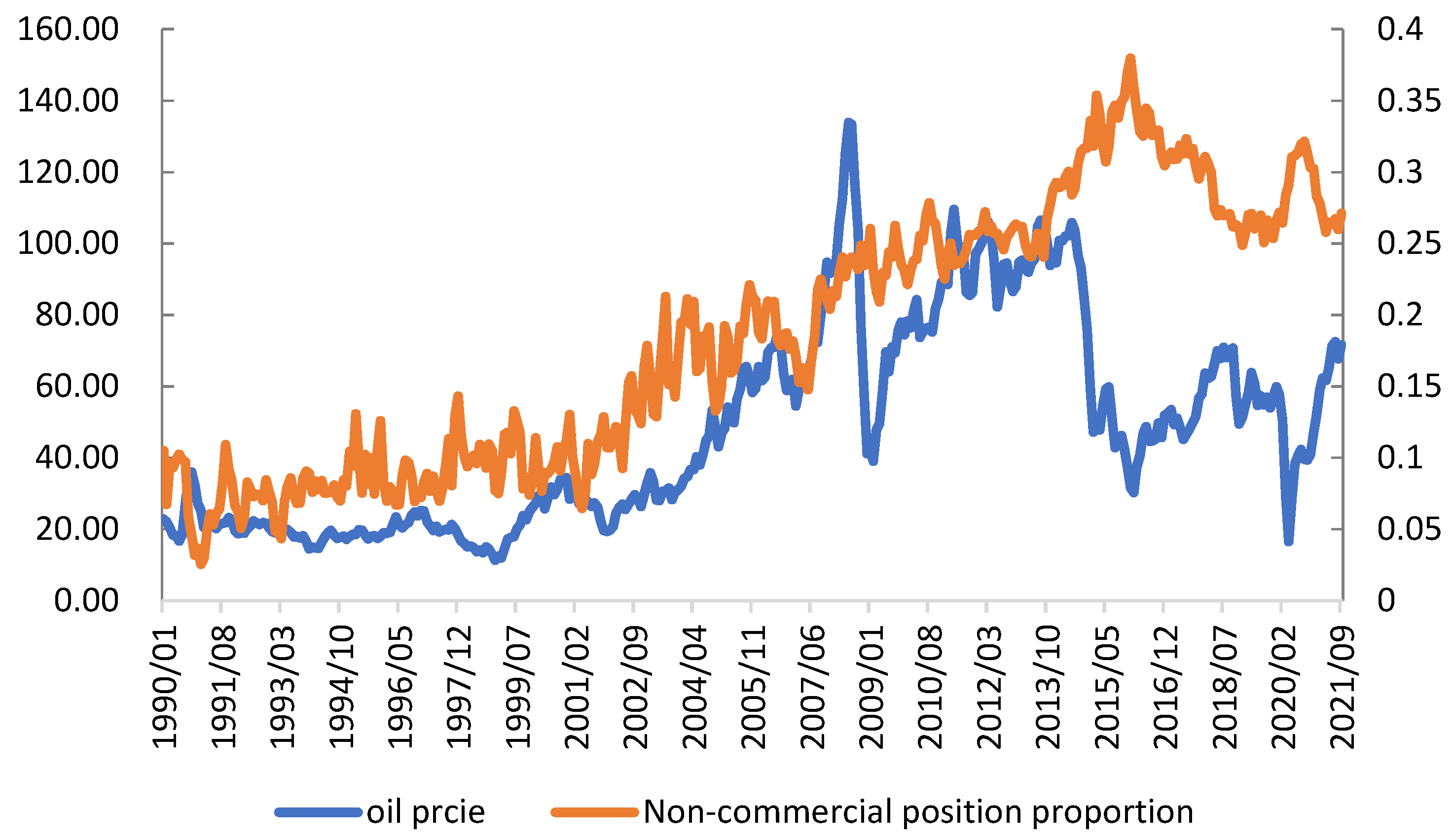
In fact, crude oil has multiple attributes, including as a commodity, and in finance and politics. It is affected by multidimensional factors and has different pricing mechanisms at different times. Therefore, the impact of oil financialization on crude oil price fluctuation may vary at different time points or in different periods. On the one hand, Wen et al. [13] found that the impact of various financial factors on crude oil price fluctuations changed over time, and the US dollar was the leading factor affecting oil prices before the crisis, but speculation became the most powerful factor after the crisis. On the other hand, the statistics show that there are significant differences in the correlation between the non-commercial position proportion in the international oil futures market and the international oil price in terms of time periods. As shown in Figure 1, after the 1990s, the international crude oil price fluctuated frequently and intensified with an upward trend. Generally speaking, the international oil price has gone through four historical stages. The first stage was 1990–2003, when the oil price experienced a period of adjustment and hovered below USD 30. The second stage was 2003–2008, when the oil price in the context of globalization surged again, presenting a straight-line upward trend. The third stage was 2009–2019, which was the adjustment period after the financial crisis. The fourth stage was 2020–2021, which was the adjustment period to the impact of the COVID epidemic. In contrast, in the international oil futures market, the non-commercial position proportion (NCPP, unit: %) remained basically stable from 1990 to 2003, rose rapidly after 2003, and showed a downward trend in 2016. It can be seen that from 1990 to 2014, the trend of oil financialization was basically consistent with the oil price, but from 2015 to 2021, it was opposite to the oil price trend. Based on this, the first goal of this paper is to empirically study the heterogeneous impact of oil financialization on oil price fluctuation in different periods. This research can not only explain the crude oil market volatility caused by oil financialization, but also provide a scientific reference for policy making and investment decision making.
In particular, the different response of oil price fluctuation to oil financialization shocks is unclear under the instantaneous impact of different major events. Due to the inherent differences in the nature and causes of different events, the combination of major events and oil financialization will lead to different effects in terms of oil financialization affecting oil price fluctuation. In addition, different major events have various impacts on the supply and demand in the crude oil market and the investment sentiment. Furthermore, the interaction mechanisms between market supply, demand, investment sentiment, and oil financialization are also different. Therefore, the instantaneous impact of oil financialization on oil price fluctuation varies with event types. For example, the global financial crisis affects the impact of oil financialization on oil price fluctuation through the financial derivatives market; geopolitical tension leads to changes in the relationship between oil supply and demand in the spot market, which in turn trigger the impact of oil financialization on oil price fluctuation; the global epidemic has an impact on the global economy and then affects the relationship between oil supply and demand and speculation, thus affecting the relationship between oil financialization and oil price fluctuation. However, this situation has not received enough attention. Therefore, the second goal of this paper is to explore the heterogeneity of the impact of oil financialization on crude oil price fluctuation when different major events occur.
In addition, we also raise the question: what is the difference between the impacts of oil financialization on high-frequency and low-frequency oil price fluctuations? In the long run, the oil pricing power is transferred to the oil derivatives market in the context of oil financialization, and international financial monopoly capital can influence oil price by its financial strength in the derivatives market. The abundant liquidity in the oil market sometimes masks the expression of the correlation between supply and demand, causing the oil price to show a trend away from supply and demand. In the short term, the sharp increase in the capital volume in the oil futures market under the trend of financialization magnifies the impact of basic supply and demand factors on medium- and long-term oil prices, causing the oil price fluctuation to increase. However, the specific differences in the impact of oil financialization on crude oil price fluctuations of different frequencies or cycles are not clear. Therefore, the third goal of this paper is to compare the responses of high-frequency and low-frequency crude oil price fluctuations to the shock of oil financialization.
The main contributions of this paper are as follows. Firstly, the biggest one is to explore the impact of oil financialization on crude oil price fluctuation from the perspective of heterogeneity. On the one hand, existing studies mainly focus on the impact of oil financialization on oil price fluctuation from a static perspective, not giving enough attention to the heterogeneity in the time dimension. On the other hand, the existing studies do not reach consensus on the view that oil financialization drives crude oil price fluctuation, which may be related to the heterogeneous correlation between oil financialization and crude oil price fluctuation. Therefore, this paper focuses on the heterogeneous impact of oil financialization on oil price fluctuations in the time dimension. Secondly, this paper studies the heterogeneous impact of oil financialization on oil price fluctuation with different frequencies. The existing studies do not discuss the impact on oil price fluctuation from the perspective of different frequencies. To this end, this paper adopts the Ensemble Empirical Mode Decomposition (EEMD) to decompose the oil price fluctuation and studies the impact heterogeneity of oil financialization on short-term and long-term oil price fluctuations. In addition, based on time-varying characteristics, this paper combines major events to analyze the instantaneous heterogeneous impact of oil financialization on crude oil price fluctuation. Major events have a considerable instantaneous impact on crude oil price fluctuation. At the same time, major events themselves have different natures, resulting in different financial speculation, which leads to oil financialization having different impacts on oil price fluctuations. This paper divides major events into three types—economic events, political events, and social events—and selects representative events to compare the heterogeneity of instantaneous shocks.
The rest of this paper is arranged as follows. Section 2 is a brief literature review. Section 3 sets out the Time-Varying Parameter Vector Auto-Regression (TVP-VAR) model, calculates the core variables, and analyzes the selection of other variables. Section 4 analyzes the results of the heterogeneous impact of oil financialization on oil price fluctuations in different time periods. Section 5 discusses the heterogeneity from the perspective of different frequencies and different events. Section 6 draws the conclusion.
2. Literature Review
Since the sharp expansion of commodity markets in 2003, the relationship between commodity speculation and its physical prices has attracted particular attention. In a special report submitted to the US Congress, Masters believed that excessive speculation is an important reason for price fluctuations [14]. Irwin and Sanders called this conclusion the “Masters Hypothesis” [15]. Then, many people are not satisfied with the explanation given by the views of commodity fundamentals. Under the waves of commodity financialization, the impact of oil speculation or oil financialization on oil price fluctuation has been warmly discussed in academic circles, as oil is an energy of great strategic significance.
Firstly, the existing research mainly comprises the following two views. On the one hand, oil speculation is related to oil price fluctuation. Cifarelli and Paladino believe that speculation plays an essential role in the oil market, which is not completely driven by fundamental factors, and monitoring market speculation is an effective measure to stabilize oil price fluctuation [16]. By exploring the impact of fundamental and speculative factors on the ups and downs of the oil prices from 2007 to 2008, Kaufmann affirmed that these two kinds of factors act jointly on oil price fluctuations [17]. Lombardi and Robays and Manera et al. measured the effect of financial speculation on crude oil prices, and found that only short-term speculation had an impact on oil price fluctuations [18,19]. Eickmeier and Lombardi concluded that financial speculation could directly affect oil prices [20]. Adams et al. held that the financialization of the crude oil market fundamentally changes the trend of oil prices and becomes the main driving factor in explaining the changes in crude oil returns and volatility [21]. In addition, some scholars have also studied the impact of oil speculation on oil price fluctuation during the financial crisis. For example, Hache and Lantz studied the relationship between crude oil futures prices and speculation and found that non-commercial participants played a significant role in the financial crisis [22]. Ding et al. found a correlation between net position and crude oil futures price [23]. Juvenal and Petrella, Li et al., and Wen et al. supported the argument that speculation led to a sharp rise in crude oil futures prices in 2008 [13,24,25]. On the other hand, oil speculation has no or a weak impact on oil price fluctuations. Kilian and Daniel believe that the surge in oil prices in the middle of 2003–2008 is mainly driven by the impact of oil demand, and all speculative transactions in the crude oil spot market have little impact on the actual price of crude oil [6]. Similarly, Knittel and Pindyck found that speculative factors has only a weak impact on commodity price fluctuations based on an equilibrium model [26]. To some extent, the two different conclusions may imply the existence of heterogeneity. Therefore, it is necessary to study the impact of oil financialization on oil price fluctuation from the perspective of heterogeneity.
Secondly, there are great differences in the selection of research methods in the existing literature. Relevant research can be roughly divided into the following categories according to the methods. The first is the research based on the GARCH family models. Manera et al. studied the impact of speculation on oil price fluctuations by constructing a GARCH model [19]. Cifarelli and Paladino analyzed the dynamic impact of speculation on oil prices using CCC GARCH-M model with complex nonlinear conditional mean equations [16]. Manera et al. employed the GARCH model to conduct a weekly analysis of four energy commodities (light low-sulfur crude oil, fuel oil, gasoline, and natural gas) from 2000 to 2014 [27]. The second kind of research uses the risk-averse arbitrage model. For example, Hamilton and Wu found that the sharp fluctuation of crude oil futures price is related to the large number holding of oil commodity index-fund [28]. The third is to study the impact of oil speculation on oil price fluctuation based on the Granger causality test [23]. Besides that, Ma et al. used the generalized dynamic factor model to predict the oil price volatility, and found that the financial factors have the most predictive power [29]. However, few studies have adopted the TVP-VAR model to study heterogeneity in the time dimension.
In addition, there are various measures of speculation in the oil futures market. It mainly includes the Working’s T index, that is, the ratio of non-commercial position to total commercial position [30]; the proportion of net long position held by speculators and the current futures trading price [19]; the commodity index fund of long crude oil futures contracts [28]; and the non-commercial net long position [13,23]. Alquist and Gervais questioned the effectiveness of using the increase in oil futures market position to explain the sharp rise in oil prices [31]. The reason for this is that the position of crude oil futures is that of the stock data, and the position of the futures market is much larger than the daily oil consumption of the United States. Therefore, it is misleading to compare the two statistics. However, according to Bruno [32], Working’s T index measures the relative size of non-commercial positions in excess of commercial hedging requirements, which are largely contributed by financial investors. Hence, the Working’s T index can better measure oil financialization.
3. Model and Data
3.1. Model Setting
The TVP-VAR model is an extension of the traditional VAR model [33]. It can serve as a helpful tool for studying the dynamic links between time-varying variables under structural shocks in a flexible and robust manner [34]. Therefore, referring to the study of Feng et al. [35], we chose the TVP-VAR model to capture the heterogeneous impact of oil financialization on oil price fluctuation in the time dimension.
Not only oil supply and demand and geopolitical factors, but also the level of oil financialization can induce the fluctuation of international oil price. This paper selects five influencing factors of oil price fluctuation: the US dollar, geopolitics, oil demand, oil financialization, and oil inventory. Furthermore, we establish a six-variable frame model. There are two main reasons for determining the order of variables: on the one hand, according to theoretical analysis, the dollar is a relatively exogenous variable, while the oil price fluctuation is a relatively endogenous variable. Therefore, in the TVP-VAR model, the US dollar should be placed in the front position, and the oil price fluctuation should be placed in the back position. On the other hand, following the common practice [36], based on the results of the Granger causality test (see Appendix A), we finally determine the order of variables as the US dollar (dol), geopolitics (geo), oil demand (dem), oil financialization (FIN), oil inventory (inv), and oil price fluctuation (OPF).
The P-order TVP-VAR model set in this paper is as follows:
where ; ; and are order vectors; the coefficients , and the parameters , and are diagonal matrices; is the diagonal elements of . Following the research of Primiceri [33], it needs to assume that the parameters in the TVP-VAR model obey random-walk processes to capture the time-varying nature of the underlying structure in economies. Let , which represents a stacked vector of the lower-triangular elements in ; with , for .
Thus,
For , where , and .
Furthermore, we assume that shocks are not related to the time-varying parameters, and the covariance matrices , , are supposed to be diagonal.
In the Bayesian frame, the model’s estimation can be constructed by using the Markov Chain Monte Carlo (MCMC) method. There are several reasons for its appropriateness. First, the model includes the nonlinear state equations of stochastic volatility, which solves the problem of the intractability of the likelihood function. Second, the method makes full use of the uncertainty of the unknown parameters to infer the state variables and estimate the function of the parameters. Lastly, these estimates are more efficient if focusing on the time-varying nature of the unobservable states, which are the issues we address in this paper.
3.2. Measurement of Core Variables
Considering the availability and consistency of data, the data frequency in this paper is unified as monthly, and the period is from January 1990 to October 2021. The main reasons are as follows. First, the crude oil inventory data we collect starts from January 1990. Second, the global economic activity index currently collected ends in October 2021.
3.2.1. Measurement of Oil Financialization
Among the studies on oil financialization or speculation in the oil futures market, most adopt the data provided by the US Commodity Futures Trading Commission (CFTC) to construct speculation indicators, such as Working’s T index. Other scholars use the price difference between oil futures and spot to measure speculation, or use the model residuals to represent the factors of financial speculation. Referring to the practices of most studies [31,32,37], this paper adopts Working’s T index, that is, the ratio of non-commercial position to total commercial position, as the proxy variable of oil financialization, and its calculation formula is as follows:
where , , , respectively represent the non-commercial short position, the non-commercial long position, the commercial long position and the commercial short position of oil futures at time t. When the proportion of non-commercial positions is at a low level, it means that the participation of financial speculative funds is low and the degree of oil financialization is weak; on the contrary, when the proportion of non-commercial positions increases, it means that the degree of oil financialization is deepened and the financial attribute of crude oil is enhanced. It should be noted that the calculation of the Working’s T index depends critically on the classification of market operators between hedgers and speculators. The CFTC publicly reports the position data of two types of dealers: commercial dealers and non-commercial dealers. Commercial dealers are considered hedgers, while non-commercial dealers are considered speculators.
3.2.2. Measurement of Crude Oil Price Fluctuation
This paper selects the monthly FOB of WTI crude oil released by the US Energy Information Administration (EIA). The sample period is from January 1990 to October 2021. To reduce the error, firstly, the oil price is obtained by logarithmic processing [38]. Considering that the price in the financial market generally follows the random walk model, the following mean equation is established for the international oil price ():
By estimating and testing Model (4), it is found that its fitting effect is good. In addition, all Q-statistics are not 0 significantly (see Appendix B), indicating that there is a high-order ARCH effect in the residual term.
The ARCH model family is the most common method for extracting or predicting future volatility based on historical information. Among the members of this family, the GARCH model is suitable for describing the high-order ARCH process conveniently when the calculation amount is not large, so it has greater applicability. Therefore, referring to the practices of Özdurak [39], and Wu and Ma [40], this paper uses a univariate GARCH model to extract crude oil price fluctuation. The general form of the generalized conditional heteroskedasticity model GARCH(p,q) is as follows:
Equation (5) is the distribution assumption, and Equation (6) is called the conditional variance equation; is the conditional variance, that is, the conditional volatility; is the independent and identically distributed random variable; and are independent of each other, and is of the standard normal distribution.
On the basis of the AIC and SC information criteria, we select GARCH(1,1), and its conditional variance sequence is used to represent the international oil price fluctuation.
3.2.3. Selection of Other Variables
In addition, other variables involved in this research are as follows. (1) The US dollar index. The US dollar is the currency often used in the international crude oil trade. Therefore, the crude oil price fluctuation is related to the exchange rate [1]. Scholars like Aloui et al., Thalassinos et al., and Jawadi et al. have pointed out that there is a correlation between the crude oil futures price and the US dollar [41,42,43]. Therefore, this paper selects the real effective US dollar exchange rate index published by the Bank for International Settlements (BIS). (2) The crude oil demand. According to the theory of commodity market price determination, the change of crude oil supply and demand can explain its price fluctuation to a great extent. Kilian [3] distinguished the impact of crude oil demand and crude oil supply in the change of oil price, and he claimed that the rise of oil price is mainly driven by the oil demand. Following the practices of Wei et al. [44] and Feng et al. [45], we select the global economic activity index compiled by Kilian and Park as the proxy variable of the oil demand [46]. (3) The crude oil inventory. The two oil crises in the last century dealt a painful blow to the economic development of western developed countries. Therefore, large countries that rely heavily on oil imports set up oil stocks. Oil inventory plays a buffer role between oil supply and oil demand; that is, it mainly acts as a regulator of the oil supply and demand. (4) The geopolitical factor. Geopolitical risks will lead to the differences in expectations of future oil supply and demand between crude oil exporting and importing countries, affecting the current oil inventory decision and price [2,4,5,47,48]. Referring to the research of Liu et al. [5], Caldara and Lacoviello [49], Li et al. [50] and Miao et al. [51], this paper selects the global geopolitical risk index (GPR) to measure the geopolitical factor. The variables above all and data sources are shown in Table 1.
To reduce error, logarithmic treatment of the crude oil inventory is carried out, and the geopolitical risk index, the oil demand (Kilian_index), and the US dollar index are divided by 100. The descriptive statistics of each variable are shown in Table 2.
4. Results
4.1. Data Preprocessing
Stationary time series are necessary for the stability of the TVP-VAR model, so a unit root test for all variables is required. The results show (Table 3) that in the original data, the unit root test of the inventory (inv) and the US dollar (dol) accept the null hypothesis, and there is a unit root. Therefore, in order to avoid the problem of information loss easily caused by differential data, it is necessary to carry out a cointegration test to determine whether there is a long-term cointegration relationship among variables. If the cointegration relationship exists, the TVP-VAR model can be estimated with the original data. The results of the Johansen cointegration test in Table 4 show that there is at least one cointegration relationship among the variables. Therefore, the original series are used to estimate the TVP-VAR model.
4.2. Heterogeneous Impacts of Oil Financialization on Oil Price Fluctuation in Different Time Periods
The impact of oil financialization on crude oil price fluctuation is time-varying. We select the Bayesian method to estimate the model. Combined with the AIC and SC criteria, this paper constructs a TVP-VAR model with 2-order lag. To calculate the posterior estimate, we set M = 10,000 times, discarding the first 1000 MCMC samples. At the 5% significance level, the diagnostics value of Geweke CD is less than the critical value, which means that the sample convergence is good. The invalid factors of the parameters are very small, indicating that the effectiveness of the state variables and parameter sampling is good, and the model estimation results meet the requirements.
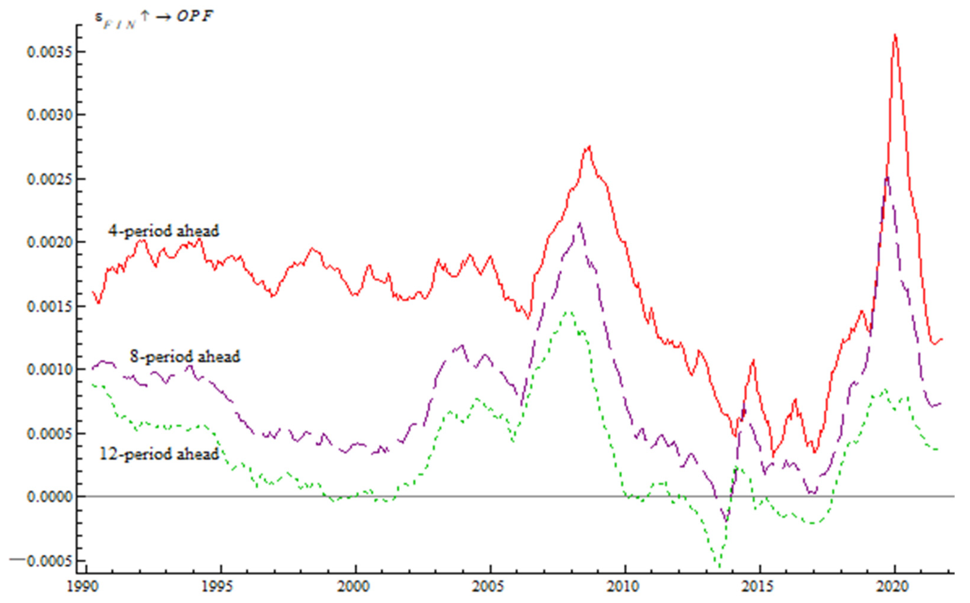
Considering the term characteristics of each variable, this paper selects the period horizons of 4 months, 8 months and 12 months to represent the short-term, medium-term and long-term effect, respectively. As can be seen from Figure 2, the impact of oil financialization on crude oil price fluctuation gradually decreases with the period horizon at all time points. In addition, on the whole, the impact of oil financialization on crude oil price fluctuation is heterogeneous in the time dimension, mainly manifested in the following two aspects.
First, the impact of oil financialization on oil price fluctuation has different fluctuation amplitudes in different periods. This heterogeneity can be divided into intervals by two events: the global financial crisis in 2008 and the global outbreak of the COVID epidemic in 2020. Firstly, before the global financial crisis, the impact of oil financialization on oil price fluctuation was relatively stable in the short, medium, and long terms. Secondly, during the financial crisis, the impact fluctuated greatly, presenting an inverted V shape; that is, it rose sharply at first and then decreased sharply. Then, after the financial crisis, the impact gradually recovered. Finally, during the global outbreak of the COVID epidemic in 2020, the impact once again showed a deep inverted V-shape. This indicates that the impact of oil financialization on oil price fluctuation will produce violent fluctuations during major events such as the financial crisis and the public-health crisis, in the specific form of first sudden increase and then sudden decrease. The reasons are as follows. First, in the first half of 2008, speculative funds entered the oil futures market, with non-commercial net positions up to 113,000 lots, which promoted the sharp rise in oil prices. As oil prices rose, speculative capital gradually reduced positions. After the oil price reached a historic high in mid-July 2008, speculative capital was reduced to net short positions in the futures market. Then, since May 2009, with the emergence of signs of global economic recovery, investment funds built positions again and returned to the market, stopping the downward trend of international oil prices. This is consistent with the research conclusions of Wen et al. [13]. Second, according to the data analysis of the US EIA, due to the impact of the COVID epidemic, the global economy is sluggish, and the oil market is oversupplied, resulting in the open positions and daily trading volume of crude oil futures contracts close to a record high in March 2020. In particular, on 20 April 2020, when the storage space in the US crude oil market was running out, the storage cost exceeded the oil price, and speculators could not find a storage place for the physical oil, speculators had to sell desperately to avoid physical delivery even if they had to pay to liquidate their positions, leading to the negative oil price. It can be seen that the level of oil financialization changes rapidly during major emergencies such as the financial crisis or the COVID epidemic, leading to sharp fluctuations in oil prices.
Second, the impact intensity of oil financialization on oil price fluctuation varies in different time periods. On the one hand, in terms of the short and medium term (for 4-period and 8-period horizons), the impact intensity of oil financialization on oil price fluctuation was the greatest during the COVID pandemic in 2020, followed by that in the financial crisis period (i.e., 2007–2009), before the financial crisis (i.e., 1990–2006), and after the financial crisis period (i.e., 2010–2019). On the other hand, from a long-term perspective (for 12-period horizon), the impact of oil financialization on oil price fluctuation was the greatest during the financial crisis period (i.e., 2007–2009), followed by the period of the COVID pandemic, the Gulf War (i.e., 1990–1991), and the eve of the financial crisis (2003–2006), then the period 1992–1994, the post-financial crisis period (i.e., 2010–2019), and finally the period 1995–2002. This shows that oil financialization has a more substantial impact on oil prices during periods of abnormal oil price fluctuation due to unexpected events, such as financial crises or epidemics. Moreover, during the financial crisis, oil financialization had a greater long-term impact on oil price fluctuation, while during the COVID pandemic, oil financialization had a greater short- and medium-term impact on oil price fluctuation [52].
4.3. Robustness Test
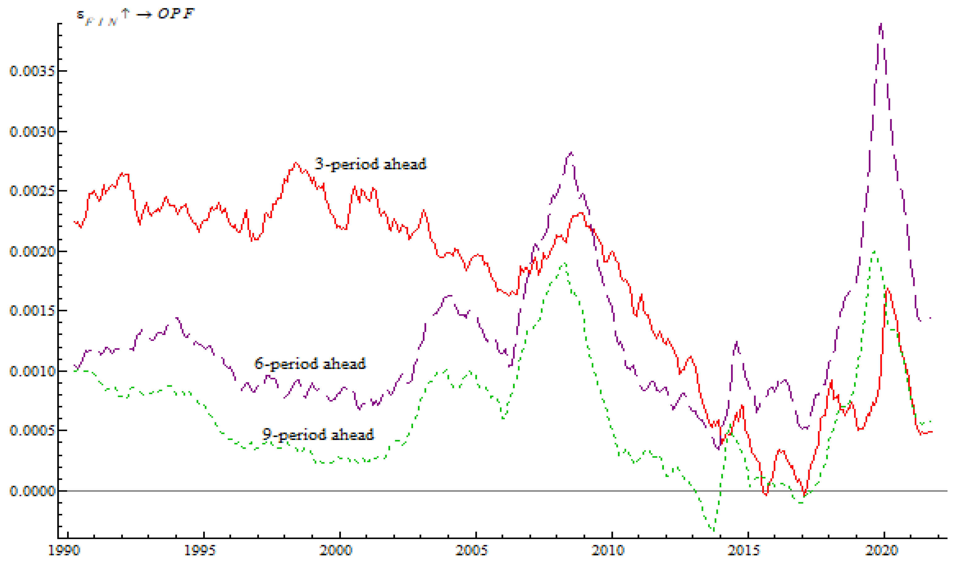
To confirm the reliability of the above conclusions, we further conduct some robustness testes. Firstly, we try to analyze the robustness of TVP-VAR models by repeating the exercise with different period horizons. In this part, we select the 3-period, 6-period, 9-period horizons to represent the short-term, medium-term and long-term effect, respectively. It can be seen from Figure 3 that the impulse responses of oil price fluctuations to oil financialization shocks for different period horizons generally show same trend. Meanwhile, the trend of impulse responses in Figure 3 are very similar to those in Figure 2. Therefore, the results support the findings presented in Section 4.2.
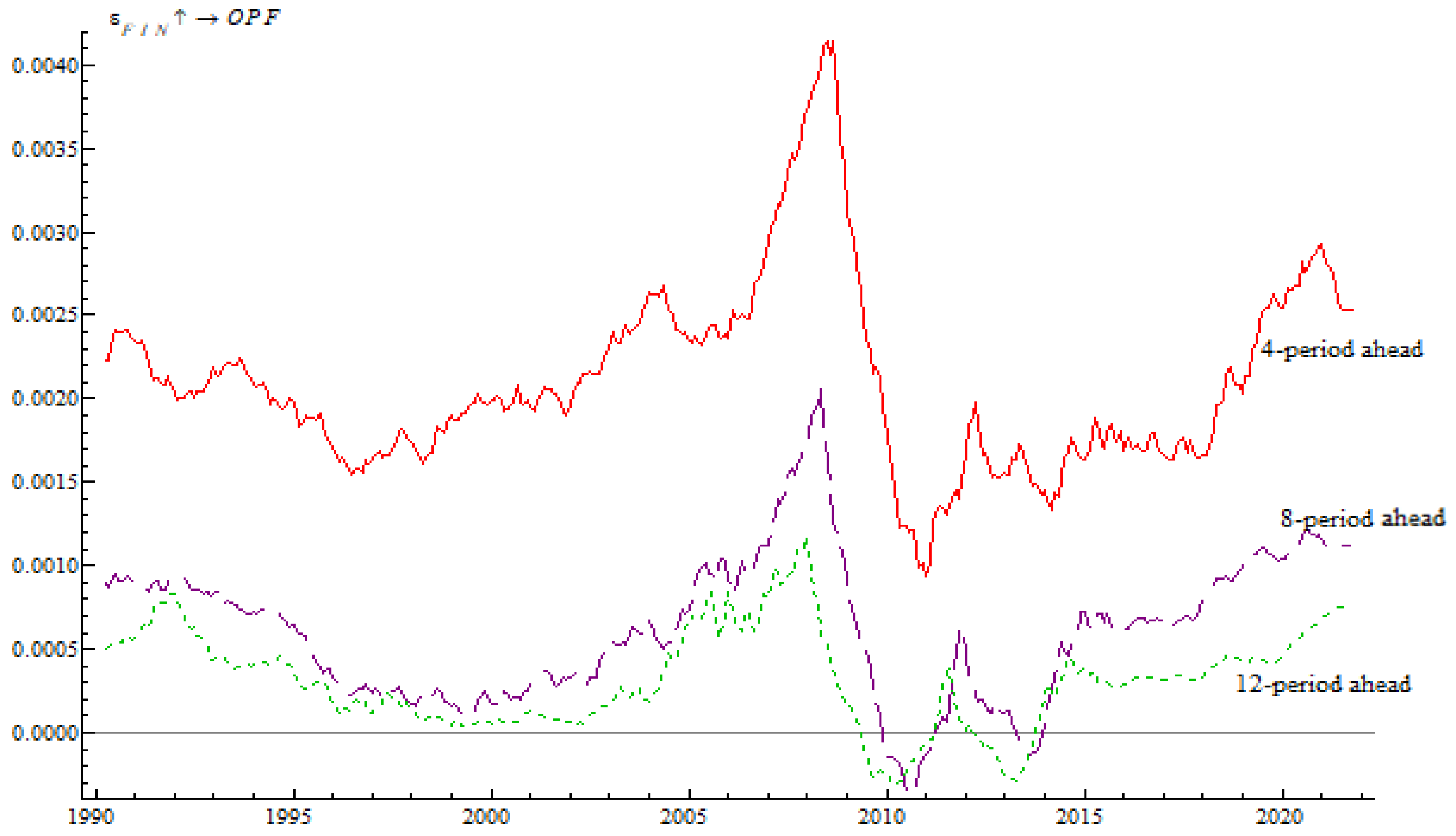
Then, we conduct a sensitivity analysis of the main results by repeating the exercise with a new set of variables. Since this paper mainly explores the impact of oil financialization on oil price fluctuation, we remove another financial factor-related variable from the model, the US dollar index. Then, the new set of variables includes geopolitics, oil financialization, oil demand, oil inventory, and oil price fluctuation. Figure 4 displays the response of oil price fluctuations to oil financialization shocks under the new set of variables. It can be found that the dynamic response of oil price fluctuation to the oil financialization shocks is not sensitive to the elimination of similar financial variables.
5. Discussion
5.1. Heterogeneous Impact of Oil Financialization on Oil Price Fluctuation at Different Frequencies
In this section, the time series of crude oil prices are decomposed into time series with different fluctuation frequencies by using the EEMD method. Then, the time series with different fluctuation frequencies are reconstructed into high-frequency and low-frequency series. After that, the TVP-VAR model is adopted to analyze the impact of oil financialization on oil price fluctuations from two scales of high frequency and low frequency.
5.1.1. Decomposition of Crude Oil Price Fluctuation Based on the EEMD
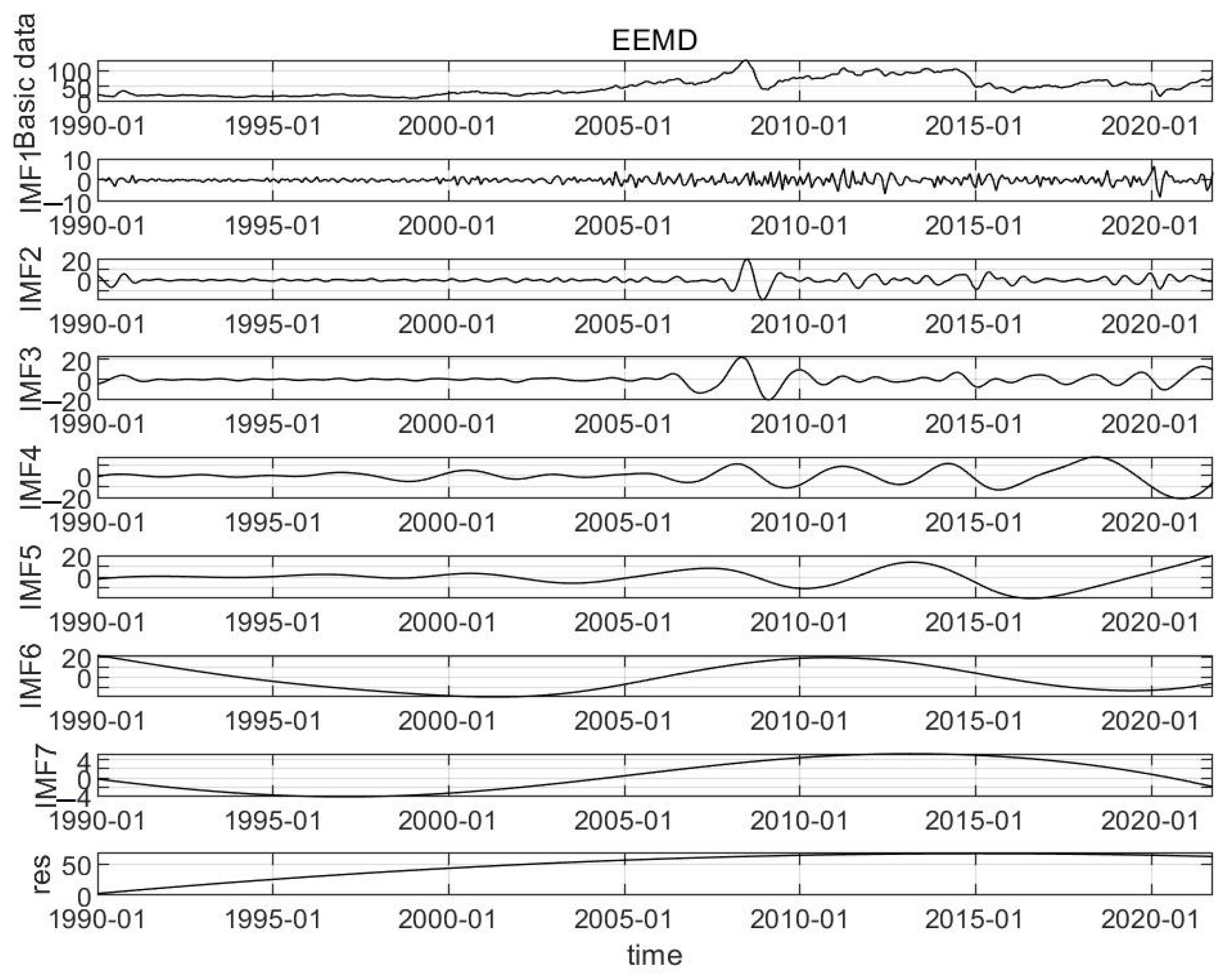
First, we decompose crude oil price fluctuation using the EEMD method. The EEMD method solves the problem of modal aliasing in the EMD method, thereby obtaining waveforms formed by different intrinsic mode function (IMF). The standard deviation of white noise is preset as , and the integration number of times is 100. Finally, the crude oil price is decomposed into eight parts; the first seven are the IMFs with different periods, and the last is the residual term generated by the decomposition. In Figure 5, each IMF is a locally symmetric fluctuation sequence with a zero mean, and the fluctuation frequency gradually decreases, while the residual term is a gently changing curve, showing no fluctuation characteristics.
Furthermore, referring to Zhang et al. [53], we adopt the zero-mean T-test analysis method to reconstruct the IMF sequences with different fluctuation frequencies. The zero-mean T-test analysis method can reconstruct multiple IMF sequences with different fluctuation frequencies into high-frequency and low-frequency sequences. In this paper, IMF1 is recorded as indicator 1, IMF1 + IMF2 is indicator 2, and so on. The sum of the first i IMFs is added as indicator i, and the mean values of indicators 1 to 7 are calculated. Then, whether the mean values are significantly different from 0 is tested by the T-test. The T-test statistic is:
where is the mean value of indicator i, is the standard deviation of indicator i, and n is the sample size of indicator i.
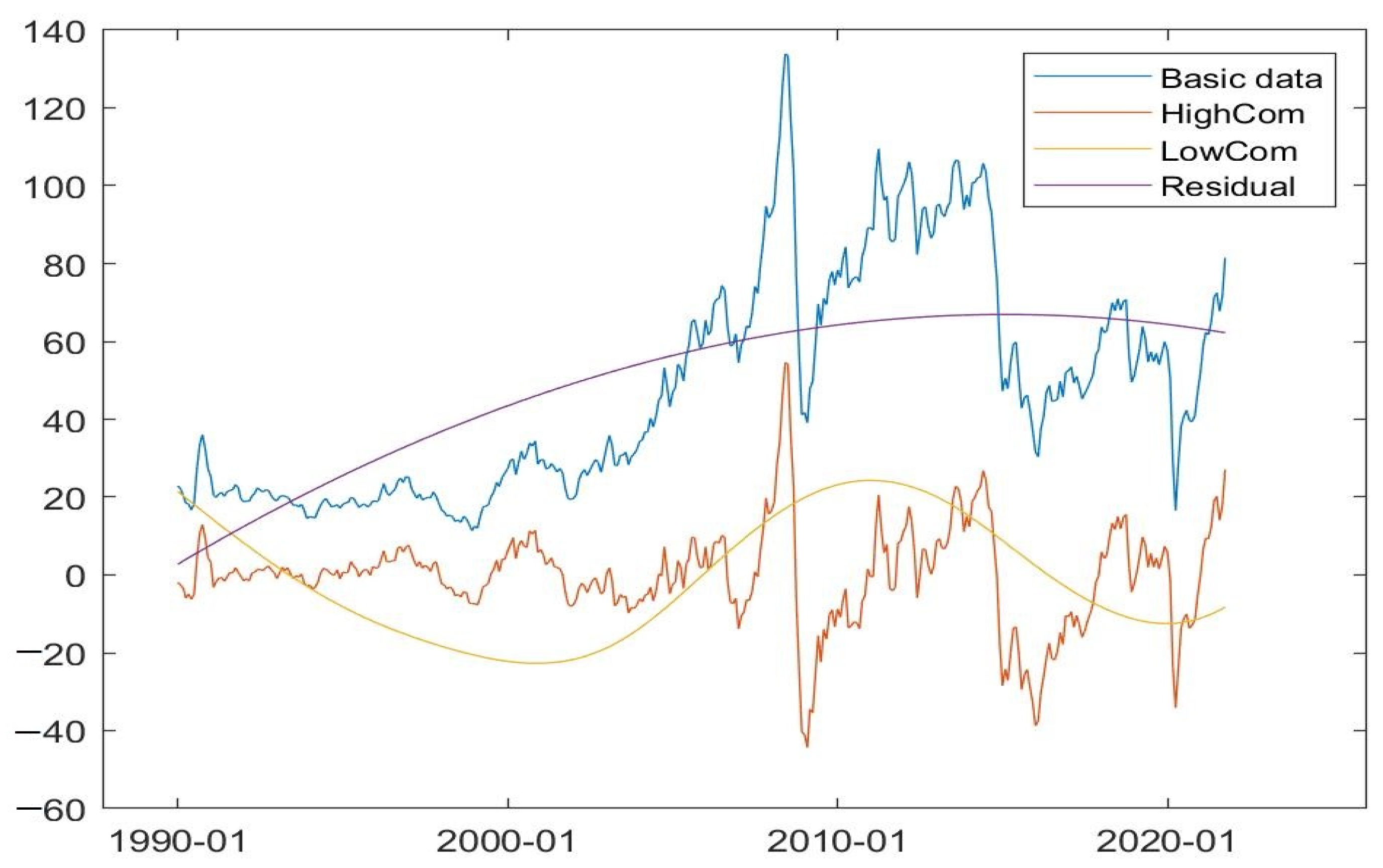
The IMF component should meet the local symmetry of the upper and lower envelope relative to the time axis. For high-frequency IMF components, the envelopes are basically obtained by connecting many signal peak points, so the symmetry of the envelope means that the IMF component data are basically symmetrical, and the data mean is close to 0. For the low-frequency IMF components, the signal period is large, and the trend of the envelope deviates greatly from the trend of the original signal. Therefore, when the envelope is symmetrical, the signal components are often asymmetrical. At this time, it is difficult to ensure that the mean value of the IMF components is 0. Generally speaking, the mean value of high-frequency components tends to be close to 0, while it is difficult for that of low-frequency components to be close to 0. Accordingly, IMF1, IMF2, IMF3, IMF4, and IMF5 are reconstructed as the high-frequency crude oil price fluctuation, and IMF6 and IMF7 are reconstructed as low-frequency fluctuations. Furthermore, the reconstructed high-frequency and low-frequency sequences are named as HighCom and LowCom, respectively. The reconstructed results are shown in Figure 6.
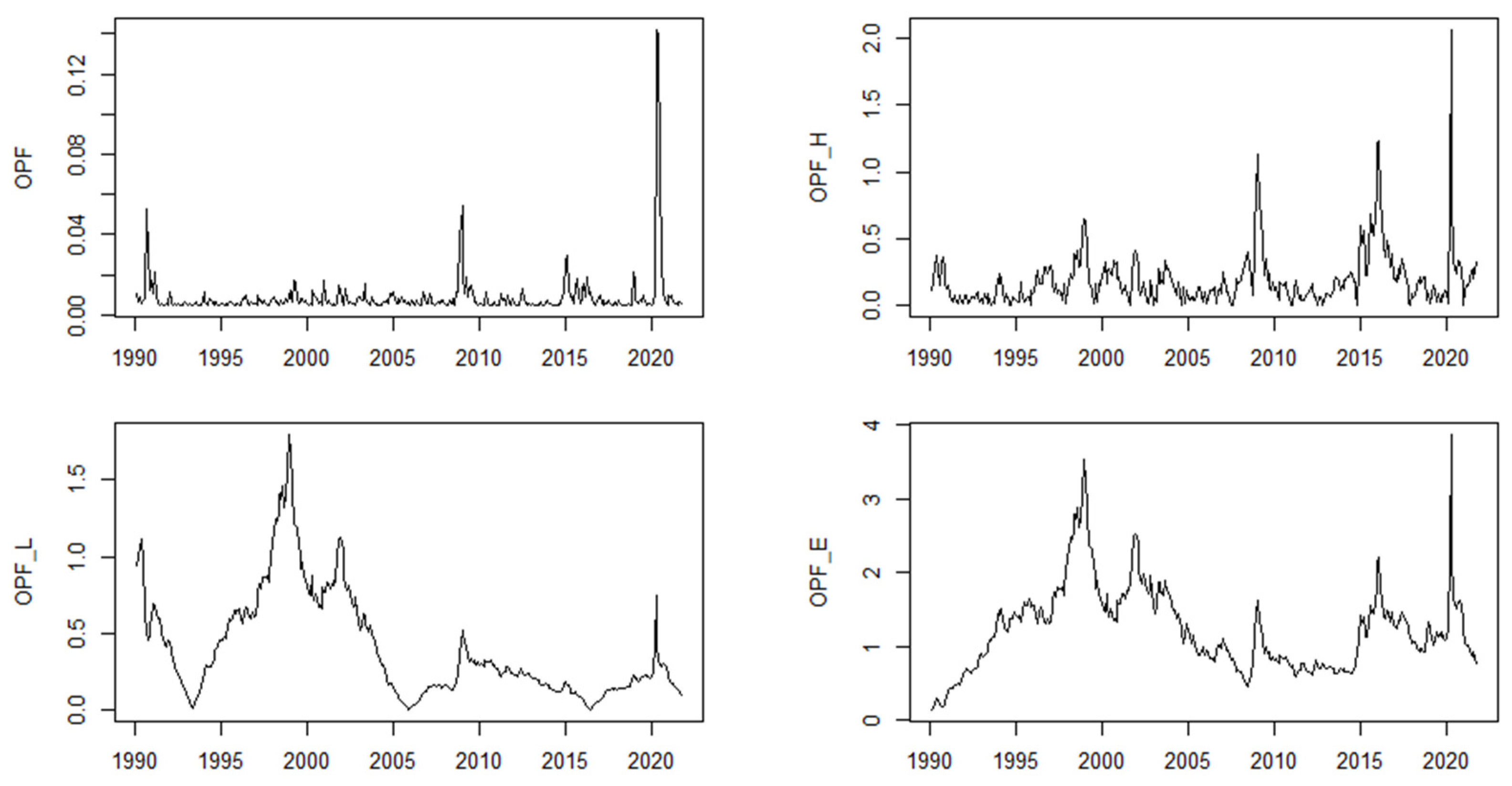
Considering the large differences in oil price on different time scales and the different contributions of each IMF fluctuation in different periods to oil price, we need a value that can measure the volatility ratio of each IMF relative to the oil price before the EEMD. Therefore, the expression of volatility is introduced. In this paper, different frequency volatility is defined as the ratio of the absolute value of IMF to the original signal at any time, namely
where is the absolute value of IMF, and is the initial signal. The volatilities of high frequency, low frequency, and the residual term are shown in Figure 7. The upper left in Figure 7 shows the volatility measured by the GARCH model. The upper right depicts the high-frequency volatility. The lower left presents the low-frequency volatility. The lower right shows the proportion of the trend item.
5.1.2. Heterogeneous Effects with Different Frequencies
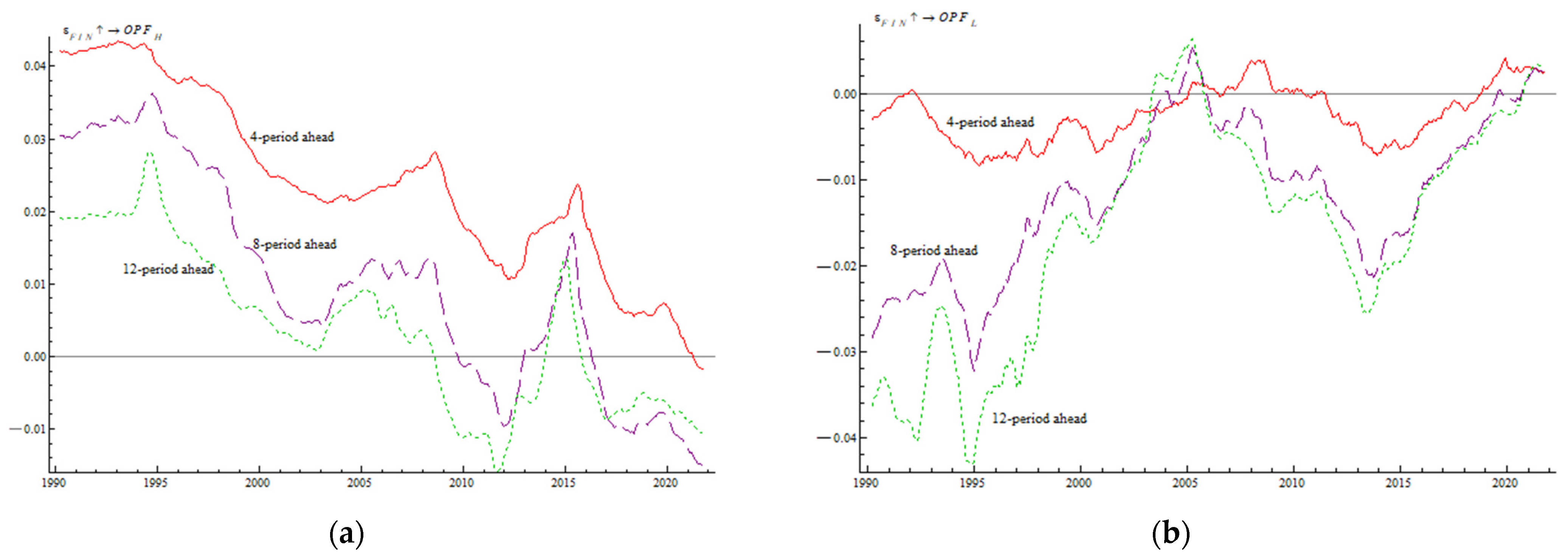
The time-varying impact of oil financialization on high-frequency and low-frequency oil price fluctuations is shown in Figure 8. It can be seen that there is heterogeneity in the impact of oil financialization on the high-frequency and low-frequency oil price fluctuations at continuous time points, mainly reflected in the following two aspects.
Firstly, oil financialization mainly promotes high-frequency oil price fluctuation and inhibits low-frequency oil price fluctuation. This is because on the one hand, in the financial market, the expectations and judgments of participants have a significant impact on the short-term changes in oil prices, and wars, conflicts, and natural disasters no longer affect the turbulence of the oil market through oil supply and transportation channels only but amplify it through the financial market. The frequent entry and exit of speculators in the oil market will cause further rise or fall in oil price in the short term, which in turn causes the high-frequency fluctuation of oil price. On the other hand, in a regulated market, speculation is subject to strict supervision and management. Speculators obtain normal economic benefits under the condition of strictly following the trading rules. Supervision and management make speculation a tool for regulating the futures market. With the participation of speculators, the trading volume of the futures market increases, and the relationship between market supply and demand can be better adjusted. According to relevant research, the commodity attribute is the first attribute of oil. In the long run, the relationship between supply and demand is the fundamental factor affecting its price [25,26]. Therefore, oil financialization can restrain low-frequency oil price fluctuations by adjusting the supply–demand relationship in the long run.
Secondly, the impact of oil financialization on high-frequency oil price fluctuations is mainly short term, while the impact on low-frequency oil price fluctuations is mainly long term. As shown in Figure 8, by comparison of different period horizons, the impact of oil financialization on high-frequency oil price fluctuations is the largest in the four-period horizon, while the impact on low-frequency oil price fluctuations is the largest in the 12-period horizon.
5.2. Heterogeneous Impact of Oil Financialization on Oil Price Fluctuation during Different Major Events
5.2.1. Heterogeneous Impact at the Time Point of Different Major Events of the Same Type
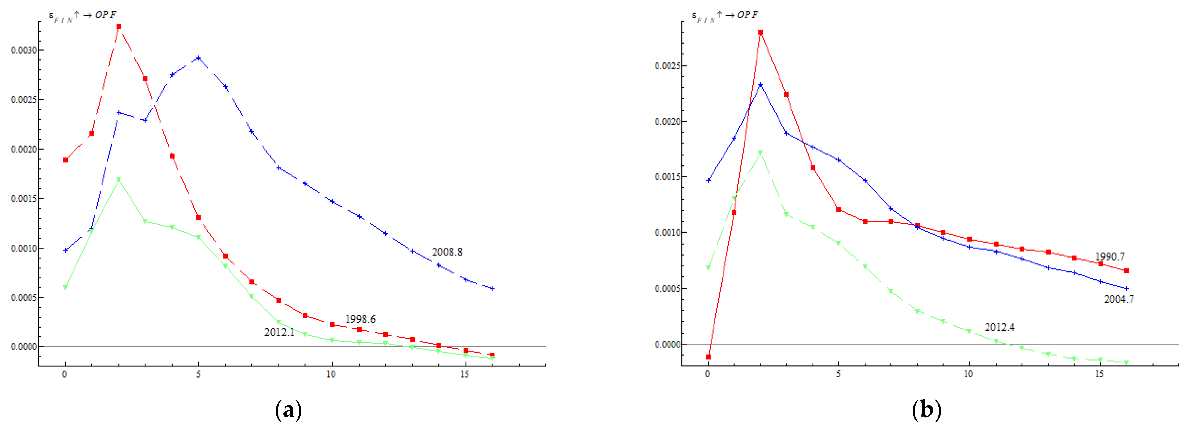
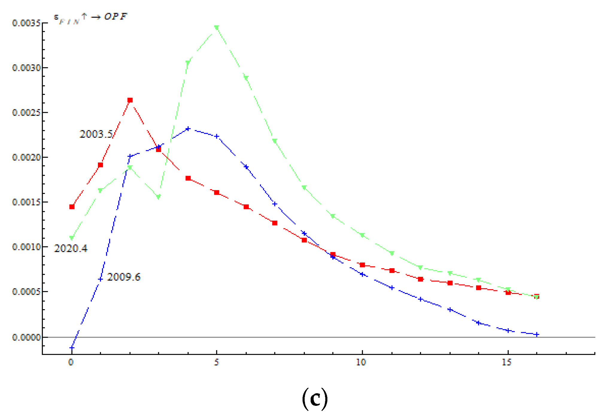
To compare the heterogeneity of the instantaneous impact of oil financialization on oil price fluctuation caused by different major events, this paper divides events into three types: economic events, political events, and social events. Firstly, this paper selects the outbreak of the Asian financial crisis in June 1998, the global financial crisis that broke out in August 2008, and the European debt crisis that broke out in January 2012 as three typical major economic events. Secondly, this paper selects three typical major political events: the Gulf War in July 1990, the Iraq War in July 2004, and the unrest in Syria in April 2012. In addition, the global epidemic of SARS in May 2003, the June 2009 global H1N1 outbreak, and the April 2020 global COVID outbreak are selected as typical social events. This paper first compares the impact of oil financialization on oil price fluctuations at different time points of the same type of different major events occurred. The impulse response at different time points is shown in Figure 9.
It can be seen from (a) in Figure 9 that the impact of oil financialization on crude oil price fluctuation is heterogeneous in terms of duration, intensity, and transmission speed with the occurrence of different economic events. In general, the larger the scale and scope of the economic event, the longer oil financialization affects crude oil price fluctuations, the greater the medium- and long-term impact intensity, and the slower the transmission speed at that time point. Specifically, first, at the time points of the Asian financial crisis and the European debt crisis, the impact of oil financialization on oil price fluctuation was almost zero, with a lag of about 15 periods, and the peak occurred at a lag of two periods, but not at the time of the global financial crisis. In addition, at the time point of the global financial crisis, the impact of oil financialization on oil price fluctuations was greater than that of the other two events, starting from five lag periods.
From Figure 9b, it can be seen that the impact of oil financialization on crude oil price fluctuation is heterogeneous in duration and intensity with the occurrence of different political events. In general, the larger the scale and scope of the political event, the longer and stronger the impact of oil financialization on crude oil price fluctuation at that time point. Specifically, first, when the turmoil in Syria occurred, the impact of oil financialization on oil price fluctuations was almost zero at a lag of 11 periods, but this was not the case for the Gulf War or the Iraq War. Second, at the time points of the Gulf War and the Iraq War, oil financialization had a greater impact on oil price fluctuation.
In addition, it can be seen from Figure 9c that the impact of oil financialization on crude oil price fluctuation is heterogeneous in terms of duration, intensity, and transmission speed with the occurrence of different social events. At the time points of the most widespread global outbreak, that of COVID, the effect of oil financialization on crude oil price fluctuations lasted longest, the medium- and long-term impact intensity was largest, and the transmission speed was slowest. This is similar to the point at which different economic events occur.
5.2.2. Heterogeneous Effects at the Time Points of Different Types of Major Event
Based on the analysis in Section 5.2.1, this paper further compares the impact of oil financialization on oil price fluctuation at the time points of different types of major event. According to the analysis results in Section 5.2.1, we select the outbreak of the financial crisis in August 2008, the outbreak of the Iraq war in July 2004 and the outbreak of the COVID epidemic in April 2020 as being representative of economic events, political events, and social events, respectively. Then, we compare the instantaneous impacts of the three types of events on oil financialization affecting oil price fluctuation.
From the comparison of the three graphs in Figure 9a–c, it can be seen that with the occurrence of three different types of event, the impact of oil financialization on crude oil price fluctuation varies with respect to transmission speed, duration, and intensity. First, with the occurrence of economic, political, and social events, the impact of oil financialization on oil price fluctuations reached its maximum in the sixth, second, and fifth lag phases, respectively. This shows that under the shock of rare political events, the impact of oil financialization on oil price fluctuation is transmitted faster, followed by the impact of social events, and finally the impact of economic events. Second, at the time point of social events, the impact of oil financialization on oil price fluctuation tends to zero in the 16th lag phase. However, when economic and political events occur, the impact lasts longer. It can be seen that the length of stable tailing of the response of oil price volatility to oil financialization shocks in the later period is directly related to the duration of the major events. Third, based on the comparison of the peaks, it can be seen that the impact at the time point of social events has the largest peak, followed by the time point of economic events, and then that of political events.
6. Conclusions
On the basis of the TVP-VAR model, this paper focuses on the heterogeneity of the impact of oil financialization on oil price fluctuation in time dimension, which is different from existing research. Based on the empirical analysis, the main conclusions obtained are as follows.
First, the impact of oil financialization on oil price fluctuation in different time periods is heterogeneous in terms of fluctuation amplitude and intensity. On the one hand, from the perspective of the fluctuation amplitude, during the global financial crisis and the global outbreak of the COVID epidemic, the impact of oil financialization on oil prices fluctuated greatly, presenting an inverted V shape, while the impact was relatively stable in the early and late stages of the global financial crisis. On the other hand, from the perspective of the impact intensity, the short- and medium-term impacts of oil financialization were the greatest during the COVID pandemic in 2020. The long-term effect was greatest during the global financial crisis.
Second, the impact of oil financialization on oil price fluctuation varies in direction and duration at different frequencies. First of all, oil financialization mainly promotes high-frequency oil price fluctuation while suppressing low-frequency oil price fluctuation. This is because on the one hand, not only does oil financialization itself have a significant impact on short-term oil price changes, but also wars, conflicts, and natural disasters can also affect short-term oil price fluctuations through the amplification of the financial market. On the other hand, the participation of oil speculators and the increased trading volume in the futures market can better regulate the relationship between oil market supply and demand. In addition, because oil is a commodity, supply and demand is the fundamental factor affecting its price in the long run. Therefore, in the long run, oil financialization can restrain low-frequency oil price fluctuation by adjusting supply and demand. Secondly, the impact of oil financialization on high-frequency oil price fluctuation is mainly short term, while the impact on low-frequency oil price fluctuation is mainly long term.
Third, the impact of oil financialization on oil price fluctuations with the occurrence of different major events is heterogeneous in terms of duration, intensity, and transmission speed. First of all, from the perspective of different major events of the same type, the larger the scale and scope of the economic event and the social event, at this time point, the longer the impact of oil financialization on the oil price fluctuation, the stronger the medium- and long-term impact, and the slower the transmission speed. The larger the scale and scope of the political event, at this time point, the longer and stronger the influence of oil financialization on the fluctuation of crude oil price will be. Secondly, from the perspective of different types of events, first, due to the shock of major political events, the impact of oil financialization is transmitted faster; second, at the time points at which economic and political events occur, the influence of oil financialization lasts longer; third, the peak of the impact of oil financialization is the largest at the time point at which the social event occurred.
From a theoretical point of view, these findings with respect to heterogeneity not only provide some new understanding of and perspectives on the relationship between oil financialization and oil price fluctuation, they also enrich the theory of the determination of oil price volatility. Meanwhile, the main policy implications of this paper are as follows. First, enterprises, governments, consumers, and speculators should pay attention to the differences in the impact of oil financialization on oil price fluctuation from multiple perspectives. Second, appropriate measures should be taken according to the situation when making decisions or formulating policies, especially when major events occur.
In addition, due to the limitations of the TVP-VAR model, this paper does not include other oil price volatility sources as mcuh as possible, and the impact mechanism is not discussed. In future research, studies employing factor-augmented dynamic models may be conducted. Furthermore, the impact mechanism of oil financialization on oil price volatility may be examined using theoretical models and time-varying parameter models.
Author Contributions
Conceptualization, S.C. and Y.F.; Data curation, Y.F., Y.L. and X.W.; Formal analysis, X.W., Y.L. and Y.F.; Investigation, S.C., X.W. and Y.F.; Methodology, X.W. and Y.F.; Resources, S.C.; Software, X.W., Y.L. and Y.F.; Supervision, Y.F., S.C. and X.W.; Validation, Y.F., S.C. and X.W.; Writing—original draft, Y.F., S.C. and X.W.; Writing—review and editing, Y.F., S.C., X.W. and Y.L. All authors have read and agreed to the published version of the manuscript.
Funding
This research was funded by National Science Foundation of Hunan Province of China (2021JJ30175).
Data Availability Statement
Not applicable.
Acknowledgments
The authors would like to thank University of South China for sponsoring this research.
Conflicts of Interest
The authors declare no conflict of interest.
Appendix A
The appendix displays the optimal lag order selection for Granger Causality Tests in Table A1, and the Granger Causality Tests results in Table A2.

Table A1.
Optimal Lag Order Selection for Granger Causality Tests.
| Lag | LogL | LR | FPE | AIC | SC | HQ |
|---|---|---|---|---|---|---|
| 0 | 2038.935 | NA | 8.59 × 10⁻¹³ | −10.75627 | −10.69381 | −10.73148 |
| 1 | 4525.409 | 4880.858 | 2.01 × 10⁻¹⁸ | −23.72174 | −23.28453 | −23.54822 |
| 2 | 4660.375 | 260.6486 | 1.19 × 10⁻¹⁸ * | −24.24537 * | −23.43341 * | −23.92312 * |
| 3 | 4694.282 | 64.40480 * | 1.20 × 10⁻¹⁸ | −24.23430 | −23.04758 | −23.76331 |
* stands for the significance level of 10%.
Table A2.
Granger causality test results.
| Null Hypothesis: | Obs | F-Statistic | Prob. |
|---|---|---|---|
| GPR does not Granger Cause USA_INDEX | 379 | 0.06177 | 0.9401 |
| USA_INDEX does not Granger Cause GPR | 4.86420 | 0.0082 | |
| KILIAN_INDEX does not Granger Cause USA_INDEX | 379 | 1.14894 | 0.3181 |
| USA_INDEX does not Granger Cause KILIAN_INDEX | 4.96000 | 0.0075 | |
| FIN does not Granger Cause USA_INDEX | 379 | 2.30424 | 0.1013 |
| USA_INDEX does not Granger Cause FIN | 0.98154 | 0.3757 | |
| INVENTORY does not Granger Cause USA_INDEX | 379 | 1.21416 | 0.2981 |
| USA_INDEX does not Granger Cause INVENTORY | 0.09047 | 0.9135 | |
| OPF does not Granger Cause USA_INDEX | 379 | 1.04866 | 0.3514 |
| USA_INDEX does not Granger Cause OPF | 0.22770 | 0.7965 | |
| KILIAN_INDEX does not Granger Cause GPR | 379 | 0.45830 | 0.6327 |
| GPR does not Granger Cause KILIAN_INDEX | 0.59741 | 0.5508 | |
| FIN does not Granger Cause GPR | 379 | 1.73582 | 0.1777 |
| GPR does not Granger Cause FIN | 0.63925 | 0.5283 | |
| INVENTORY does not Granger Cause GPR | 379 | 1.10560 | 0.3321 |
| GPR does not Granger Cause INVENTORY | 0.72451 | 0.4852 | |
| OPF does not Granger Cause GPR | 379 | 0.13689 | 0.8721 |
| GPR does not Granger Cause OPF | 1.74846 | 0.1755 | |
| FIN does not Granger Cause KILIAN_INDEX | 379 | 0.28790 | 0.7500 |
| KILIAN_INDEX does not Granger Cause FIN | 0.74715 | 0.4744 | |
| INVENTORY does not Granger Cause KILIAN_INDEX | 379 | 0.19757 | 0.8208 |
| KILIAN_INDEX does not Granger Cause INVENTORY | 0.97534 | 0.3780 | |
| OPF does not Granger Cause KILIAN_INDEX | 379 | 2.99116 | 0.0514 |
| KILIAN_INDEX does not Granger Cause OPF | 2.53637 | 0.0805 | |
| INVENTORY does not Granger Cause FIN | 379 | 3.58740 | 0.0286 |
| FIN does not Granger Cause INVENTORY | 3.61112 | 0.0280 | |
| OPF does not Granger Cause FIN | 379 | 0.35499 | 0.7014 |
| FIN does not Granger Cause OPF | 0.45393 | 0.6355 | |
| OPF does not Granger Cause INVENTORY | 379 | 1.04806 | 0.3516 |
| INVENTORY does not Granger Cause OPF | 1.19028 | 0.3053 | |
Lags: 2.
Appendix B
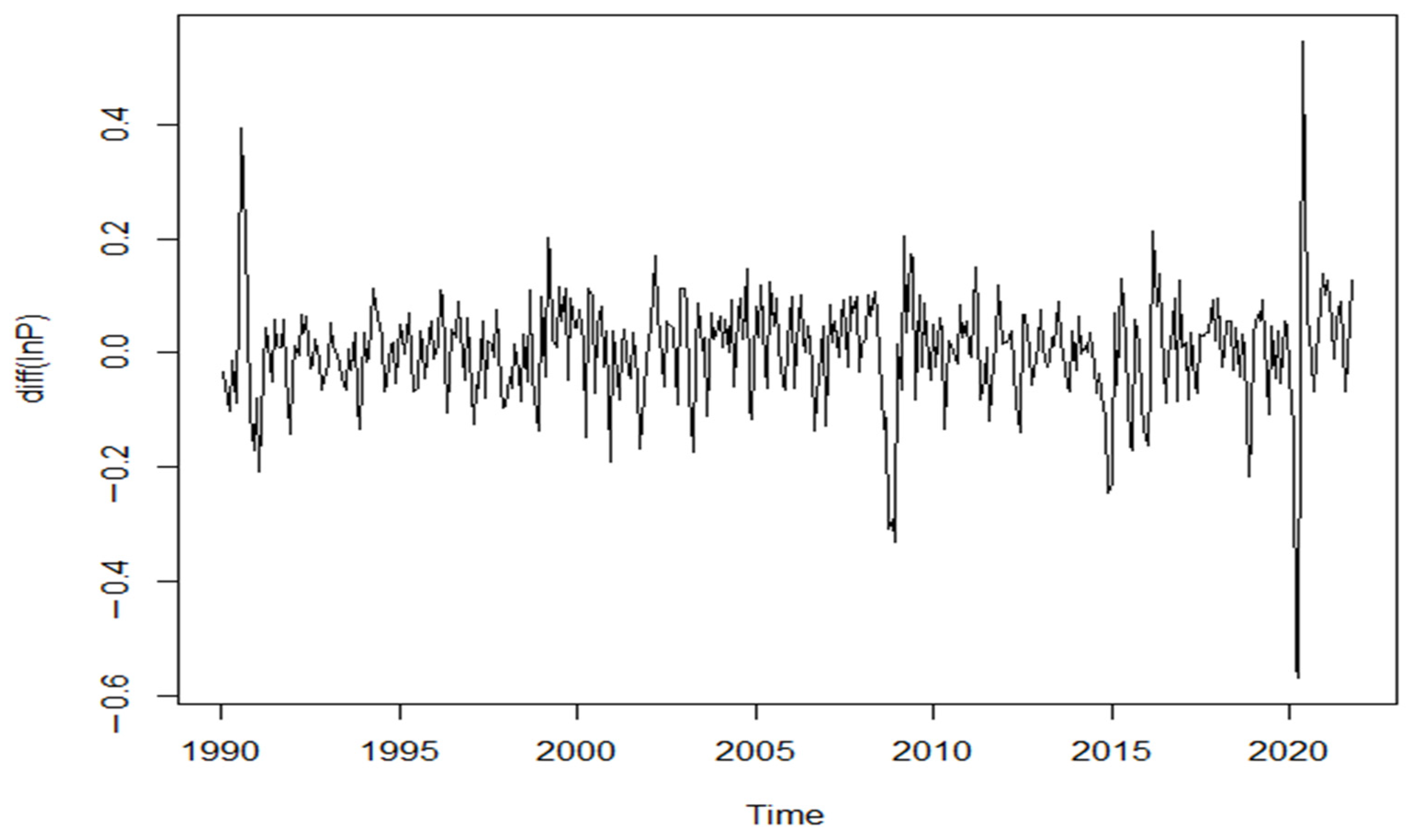
Figure A1.
Q-test of residual square correlation. Note: diff(lnP) in the figure represents the first order difference of the logarithm of oil price.
Figure A1.
Q-test of residual square correlation. Note: diff(lnP) in the figure represents the first order difference of the logarithm of oil price.

References
- Beckmann, J.; Czudaj, R.L.; Arora, V. The relationship between oil prices and exchange rates: Revisiting theory and evidence. Energy Econ. 2020, 88, 104772. [Google Scholar] [CrossRef]
- Datta, D.D.; Londono, J.M.; Ross, L.J. Generating options-implied probability densities to understand oil market events. Energy Econ. 2017, 64, 440–457. [Google Scholar] [CrossRef]
- Kilian, L. Not All Oil Price Shocks Are Alike: Disentangling Demand and Supply Shocks in the Crude Oil Market. Am. Econ. Rev. 2009, 99, 1053–1069. [Google Scholar] [CrossRef]
- Noguera-Santaella, J. Geopolitics and the oil price. Econ. Model. 2016, 52, 301–309. [Google Scholar] [CrossRef]
- Liu, J.; Ma, F.; Tang, Y.K.; Zhang, Y.J. Geopolitical risk and oil volatility: A new insight. Energy Econ. 2019, 84, 104548. [Google Scholar] [CrossRef]
- Kilian, L.; Murphy, D.P. The Role of Inventories and Speculative Trading in the Global Market for Crude Oil. J. Appl. Econ. 2014, 29, 454–478. [Google Scholar] [CrossRef]
- Nguyen, H.; Nguyen, H.; Pham, A. Oil Price Declines Could Hurt US Financial Markets: The Role of Oil Price Level. Energy J. 2020, 41, 1–22. [Google Scholar] [CrossRef]
- Bianchi, R.J.; Fan, J.H.; Todorova, N. Financialization and de-financialization of commodity futures: A quantile regression approach. Int. Rev. Financ. Anal. 2020, 68, 101451. [Google Scholar] [CrossRef]
- Tudor, C.; Anghel, A. The Financialization of Crude Oil Markets and Its Impact on Market Efficiency: Evidence from the Predictive Ability and Performance of Technical Trading Strategies. Energies 2021, 14, 4485. [Google Scholar] [CrossRef]
- Tang, K.; Xiong, W. Index Investment and the Financialization of Commodities. Financ. Anal. J. 2012, 68, 54–74. [Google Scholar] [CrossRef]
- Gong, X.; Lin, B.Q. Time-varying effects of oil supply and demand shocks on China’s macro-economy. Energy 2018, 149, 424–437. [Google Scholar] [CrossRef]
- Li, Z.; Huang, Z.; Failler, P. Dynamic Correlation between Crude Oil Price and Investor Sentiment in China: Heterogeneous and Asymmetric Effect. Energies 2022, 15, 687. [Google Scholar] [CrossRef]
- Wen, F.H.; Zhang, M.Z.; Deng, M.; Zhao, Y.P.; Ouyang, J. Exploring the dynamic effects of financial factors on oil prices based on a TVP-VAR model. Phys. A Stat. Mech. Appl. 2019, 532, 121881. [Google Scholar] [CrossRef]
- Masters, M.W. Testimony before the Committee on Homeland Security and Governmental Affairs; US Senate: Washington, DC, USA, 2008. [Google Scholar]
- Irwin, S.H.; Sanders, D.R. Testing the Masters Hypothesis in commodity futures markets. Energy Econ. 2012, 34, 256–269. [Google Scholar] [CrossRef]
- Cifarelli, G.; Paladino, G. Oil price dynamics and speculation: A multivariate financial approach. Energy Econ. 2010, 32, 363–372. [Google Scholar] [CrossRef]
- Kaufmann, R.K. The role of market fundamentals and speculation in recent price changes for crude oil. Energy Policy 2011, 39, 105–115. [Google Scholar] [CrossRef]
- Lombardi, M.; Van Robays, I. Do Financial Investors Destabilize the Oil Price? Ghent University, Faculty of Economics and Business Administration: Ghent, Belgium, 2011. [Google Scholar]
- Manera, M.; Nicolini, M.; Vignati, I. Financial Speculation in Energy and Agriculture Futures Markets: A Multivariate Garch Approach. Energy J. 2013, 34, 55–81. [Google Scholar] [CrossRef]
- Eickmeier, S.; Lombardi, M. Monetary Policy and the Oil Futures Market; Deutsche Bundesbank: Frankfurt am Main, France, 2012. [Google Scholar]
- Adams, Z.; Collot, S.; Kartsakli, M. Have commodities become a financial asset? Evidence from ten years of Financialization. Energy Econ. 2020, 89, 104769. [Google Scholar] [CrossRef]
- Hache, E.; Lantz, F. Speculative trading and oil price dynamic: A study of the WTI market. Energy Econ. 2013, 36, 334–340. [Google Scholar] [CrossRef]
- Ding, H.; Kim, H.-G.; Park, S.Y. Do net positions in the futures market cause spot prices of crude oil? Econ. Model. 2014, 41, 177–190. [Google Scholar] [CrossRef]
- Li, H.; Kim, H.-G.; Park, S.Y. The role of financial speculation in the energy future markets: A new time-varying coefficient approach. Econ. Model. 2015, 51, 112–122. [Google Scholar] [CrossRef]
- Juvenal, L.; Petrella, I. Speculation in the Oil Market. Econ. Synop. 2012, 8, 621–649. [Google Scholar] [CrossRef]
- Knittel, C.; Pindyck, R. The Simple Economics of Commodity Price Speculation. Am. Econ. J. Macroecon. 2013, 8, 85–110. [Google Scholar] [CrossRef]
- Manera, M.; Nicolini, M.; Vignati, I. Modelling futures price volatility in energy markets: Is there a role for financial speculation? Energy Econ. 2016, 53, 220–229. [Google Scholar] [CrossRef]
- Hamilton, J.D.; Wu, J.C. Risk Premia in Crude Oil Futures Prices. NBER Work. Pap. 2014, 42, 9–37. [Google Scholar] [CrossRef]
- Ma, Y.R.; Ji, Q.; Pan, J. Oil financialization and volatility forecast: Evidence from multidimensional predictors. J. Forecast. 2019, 38, 564–581. [Google Scholar]
- Working, H. Speculation on Hedging Markets. Food Res. Inst. Stud. 1960, 1, 185–220. [Google Scholar]
- Alquist, R.; Gervais, O. The Role of Financial Speculation in Driving the Price of Crude Oil. Energy J. 2013, 34, 35–54. [Google Scholar] [CrossRef]
- Bruno, V.; Buyuksahin, B.; Robe, M. The Financialization of Food? Am. J. Agric. Econ. 2017, 99, 243–264. [Google Scholar] [CrossRef]
- Primiceri, G. Time Varying Structural Vector Autoregressions and Monetary Policy. Rev. Econ. Stud. 2005, 3, 821–852. [Google Scholar] [CrossRef]
- Nakajima, J.; Kasuya, M.; Watanabe, T. Bayesian Analysis of Time-Varying Parameter Vector Autoregressive Model for the Japanese Economy and Monetary Policy. J. Jpn. Int. Econ. 2009, 25, 225–245. [Google Scholar] [CrossRef]
- Feng, Y.; Chen, S.; Xuan, W.; Yong, T. Time-varying impact of U.S. financial conditions on China’s inflation: A perspective of different types of events. Quant. Financ. Econ. 2021, 5, 604–622. [Google Scholar] [CrossRef]
- Liow, K.H.; Song, J.; Zhou, X. Volatility connectedness and market dependence across major financial markets in China economy. Quant. Financ. Econ. 2021, 5, 397–420. [Google Scholar] [CrossRef]
- Büyükşahin, B.; Robe, M.A. Speculators, commodities and cross-market linkages. J. Int. Money Financ. 2014, 42, 38–70. [Google Scholar] [CrossRef]
- Özgür, C.; Sarıkovanlık, V. An application of Regular Vine copula in portfolio risk forecasting: Evidence from Istanbul stock exchange. Quant. Financ. Econ. 2021, 5, 452–470. [Google Scholar] [CrossRef]
- Özdurak, C. Nexus between crude oil prices, clean energy investments, technology companies and energy democracy. Green Financ. 2021, 3, 337–350. [Google Scholar] [CrossRef]
- Wu, Y.; Ma, S. Impact of COVID-19 on energy prices and main macroeconomic indicators—evidence from China’s energy market. Green Financ. 2021, 3, 383–402. [Google Scholar] [CrossRef]
- Aloui, R.; Hammoudeh, S.; Nguyen, D.K. A time-varying copula approach to oil and stock market dependence: The case of transition economies. Energy Econ. 2013, 39, 208–221. [Google Scholar] [CrossRef]
- Thalassinos, E.; Politis, E. The Evaluation of the USD Currency and the Oil Prices: A Var Analysis. Eur. Res. Stud. J. 2012, 15, 137–146. [Google Scholar]
- Jawadi, F.; Louhichi, W.; Ameur, H.B.; Cheffou, A.I. On oil-US exchange rate volatility relationships: An intraday analysis. Econ. Model. 2016, 59, 329–334. [Google Scholar] [CrossRef]
- Wei, Y.; Liu, J.; Lai, X.D.; Hu, Y. Which determinant is the most informative in forecasting crude oil market volatility: Fundamental, speculation, or uncertainty? Energy Econ. 2017, 68, 141–150. [Google Scholar] [CrossRef]
- Feng, Y.; Xu, D.; Failler, P.; Li, T. Research on the Time-Varying Impact of Economic Policy Uncertainty on Crude Oil Price Fluctuation. Sustainability 2020, 12, 6523. [Google Scholar] [CrossRef]
- Kilian, L.; Park, C. The Impact of Oil Price Shocks on the US Stock Market. Int. Econ. Rev. 2009, 50, 1267–1287. [Google Scholar] [CrossRef]
- Antonakakis, N.; Gupta, R.; Kollias, C.; Papadamou, S. Geopolitical risks and the oil-stock nexus over 1899–2016. Financ. Res. Lett. 2017, 23, 165–173. [Google Scholar] [CrossRef]
- Ramiah, V.; Wallace, D.; Veron, J.F.; Reddy, K.; Elliott, R. The effects of recent terrorist attacks on risk and return in commodity markets. Energy Econ. 2019, 77, 13–22. [Google Scholar] [CrossRef]
- Caldara, D.; Iacoviello, M. Measuring Geopolitical Risk. Am. Econ. Rev. 2022, 112, 1194–1225. [Google Scholar] [CrossRef]
- Li, F.; Yang, C.; Li, Z.; Failler, P. Does Geopolitics Have an Impact on Energy Trade? Empirical Research on Emerging Countries. Sustainability 2021, 13, 5199. [Google Scholar] [CrossRef]
- Miao, H.; Ramchander, S.; Wang, T.Y.; Yang, D.X. Influential factors in crude oil price forecasting. Energy Econ. 2017, 68, 77–88. [Google Scholar] [CrossRef]
- Awan, T.M.; Khan, M.S.; Haq, I.U.; Kazmi, S. Oil and stock markets volatility during pandemic times: A review of G7 countries. Green Financ. 2021, 3, 15–27. [Google Scholar] [CrossRef]
- Zhang, X.; Lai, K.K.; Wang, S.-Y. A new approach for crude oil price analysis based on Empirical Mode Decomposition. Energy Econ. 2008, 30, 905–918. [Google Scholar] [CrossRef]
Figure 1.
Trends of Brent oil spot price and non-commercial position proportion.

Figure 2.
Time-varying impulse response of oil financialization to oil price fluctuation.

Figure 3.
Impulse response to oil financialization shock for different periods.

Figure 4.
Impulse response to oil financialization shocks under the new set of variables.

Figure 5.
EEMD results of crude oil price.

Figure 6.
Hybrid graph of the decomposition structure reconstruction.

Figure 7.
Different volatility trends.

Figure 8.
Impulse response of oil financialization to high-frequency and low-frequency oil price fluctuations. (a) High-frequency oil price fluctuation. (b) Low-frequency oil price fluctuation.
Figure 8.
Impulse response of oil financialization to high-frequency and low-frequency oil price fluctuations. (a) High-frequency oil price fluctuation. (b) Low-frequency oil price fluctuation.

Figure 9.
Impulse response at the time points of different major events. (a) Impulse response at the time points of economic events. (b) Impulse response at the time points of political events. (c) Impulse response at the time points of social events.
Figure 9.
Impulse response at the time points of different major events. (a) Impulse response at the time points of economic events. (b) Impulse response at the time points of political events. (c) Impulse response at the time points of social events.


Table 1.
Variables and data sources.
| Indicator | Abbreviation | Data Frequency | Data Sources |
|---|---|---|---|
| Non-commercial long position | NCL | Monthly | Wind Database |
| Non-commercial short position | NCS | Monthly | Wind Database |
| Commercial long position | CL | Monthly | Wind Database |
| Commercial short position | CS | Monthly | Wind Database |
| crude oil price | OP | Monthly | EIA |
| geopolitical risk index | geo | Monthly | https://www.matteoiacoviello.com/gpr.htm (accessed on 1 March 2022) |
| crude oil demand | dem | Monthly | EIA |
| crude oil inventory | inv | Monthly | Wind Database |
| US dollar index | dol | Monthly | BIS |
Table 2.
Descriptive statistics of variables.
| Variable | Obs | Mean | Std. Dev. | Min | Max |
|---|---|---|---|---|---|
| dem | 381 | 0.0265 | 0.6158 | −1.6239 | 1.8864 |
| inv | 381 | 14.3546 | 0.0893 | 14.1954 | 14.5634 |
| geo | 381 | 0.9887 | 0.4996 | 0.3905 | 5.1253 |
| FIN | 381 | 1.0757 | 0.0450 | 1.0053 | 1.2411 |
| OPF | 381 | 0.0089 | 0.0126 | 0.0044 | 0.1419 |
| dol | 381 | 0.9123 | 0.0994 | 0.7217 | 1.2059 |
Table 3.
Unit root tests of variables.
| Intercept | Trend and Intercept | |||
|---|---|---|---|---|
| t-Statistic | Prob. | t-Statistic | Prob. | |
| dol | −2.067384 | 0.2582 | −2.053257 | 0.5697 |
| geo | −6.450934 | 0.0000 *** | −6.491756 | 0.0000 *** |
| dem | −3.610397 | 0.0060 *** | −3.576527 | 0.0332 ** |
| FIN | −3.110196 | 0.0266 ** | −4.121136 | 0.0064 ** |
| inv | −1.326932 | 0.6180 | −3.734876 | 0.0212 ** |
| OPF | −9.715282 | 0.0000 *** | −9.852270 | 0.0000 *** |
Notes: Null hypothesis: the time series has a unit root; lag length: 4 (automatic—based on SIC, maxlag = 16); **, *** stands for the significance level of 5%, 1% respectively.
Table 4.
Johansen cointegration test.
| Hypothesized | Trace | 0.05 | ||
|---|---|---|---|---|
| No. of CE(s) | Eigenvalue | Statistic | Critical Value | Prob. |
| None | 0.151123 | 134.0157 | 95.75366 | 0.0000 *** |
| At most 1 | 0.085458 | 72.41125 | 69.81889 | 0.0306 ** |
| At most 2 | 0.046121 | 38.82228 | 47.85613 | 0.2674 |
| At most 3 | 0.031727 | 21.06813 | 29.79707 | 0.3534 |
| At most 4 | 0.016588 | 8.945534 | 15.49471 | 0.3704 |
| At most 5 | 0.007039 | 2.656194 | 3.841466 | 0.1031 |
Note: **, *** stands for the significance level of 5%, 1% respectively.
Publisher’s Note: MDPI stays neutral with regard to jurisdictional claims in published maps and institutional affiliations. |
© 2022 by the authors. Licensee MDPI, Basel, Switzerland. This article is an open access article distributed under the terms and conditions of the Creative Commons Attribution (CC BY) license (https://creativecommons.org/licenses/by/4.0/).
Share and Cite
MDPI and ACS Style
Feng, Y.; Wang, X.; Chen, S.; Liu, Y. Impact of Oil Financialization on Oil Price Fluctuation: A Perspective of Heterogeneity. Energies 2022, 15, 4294. https://0-doi-org.brum.beds.ac.uk/10.3390/en15124294
AMA Style
Feng Y, Wang X, Chen S, Liu Y. Impact of Oil Financialization on Oil Price Fluctuation: A Perspective of Heterogeneity. Energies. 2022; 15(12):4294. https://0-doi-org.brum.beds.ac.uk/10.3390/en15124294
Chicago/Turabian StyleFeng, Yanhong, Xiaolei Wang, Shuanglian Chen, and Yanqiong Liu. 2022. "Impact of Oil Financialization on Oil Price Fluctuation: A Perspective of Heterogeneity" Energies 15, no. 12: 4294. https://0-doi-org.brum.beds.ac.uk/10.3390/en15124294
Note that from the first issue of 2016, this journal uses article numbers instead of page numbers. See further details here.