
Estimating Sustainable Long-Term Fluid Disposal Rates in the Alberta Basin
1
Department of Civil and Environmental Engineering, University of Alberta, Edmonton, AB T6G 2R3, Canada
2
Department of Earth and Environmental Sciences, University of Waterloo, Waterloo, ON N2L 3G1, Canada
*
Author to whom correspondence should be addressed.
Energies 2023, 16(6), 2532; https://0-doi-org.brum.beds.ac.uk/10.3390/en16062532
Submission received: 6 February 2023
/
Revised: 28 February 2023
/
Accepted: 6 March 2023
/
Published: 7 March 2023
(This article belongs to the Special Issue State of the Art Geo-Energy Technology in North America)
Abstract
:Reliable regional-scale permeability data and minimum sustained injectivity rate estimates are key parameters required to mitigate economic risk in the site selection, design, and development of commercial-scale carbon sequestration projects, but are seldom available. We used extensive publicly available disposal well data from over 4000 disposal wells to assess and history-match regional permeability estimates and provide the frequency distribution for disposal well injection rates in each of 66 disposal formations in the Alberta Basin. We then used core data and laboratory analyses from over 3000 cores to construct 3D geological, geomechanical and petrophysical models for 22 of these disposal formations. We subsequently used these models and the history-matched regional permeability estimates to conduct coupled geomechanical and reservoir simulation modeling (using the ResFrac™, Palo Alto, CA, USA, numerical simulator) to assess: (i) well performance in each formation when injecting carbon dioxide for a 20-year period; (ii) carbon dioxide saturation and reservoir response at the end of the 20-year injection period; (iii) reliability of our simulated rates compared to an actual commercial sequestration project. We found that: (i) the injection rate from our simulations closely matched actual performance of the commercial case; (ii) only 7 of the 22 disposal formations analyzed appeared capable of supporting carbon dioxide injectors operating at greater than 200,000 tons per year/well; (iii) three of these formations could support injectors operating at rates comparable to the successful commercial-scale case; (iv) carbon dioxide presence and a formation pressure increase of at least 25% above pre-injection pressure can be expected at the boundaries of the (12 km × 12 km) model domain at the end of 20 years of injection.
1. Introduction
Evolution of energy supply policies globally has the potential to fundamentally change subsurface formation pore space utilization in hydrocarbon producing basins across the globe. In the Alberta Basin, large-scale hydrocarbon fluid extraction over the last 60 years has resulted in extensive pressure depletion in most of the higher permeability (i.e., “conventional”) oil and gas formations [1]. However, emerging energy policies, such as net-zero emissions goals, can progressively increase subsurface fluid pressures in such formations, by gradually decreasing (future) fluid extraction rates while increasing (future) fluid injection rates. Additionally, reconciliation of (i) the anticipated volume of fluids to be injected into the subsurface with sustainable subsurface formation capacity, and (ii) injection rates required to support industrial needs with sustainable injection rates supported by the targeted formations are required to support optimal utilization of the existing basin subsurface pore space capacity and minimize risks to project proponents and clients as well as surface (e.g., induced seismicity) and subsurface users [1]. Extensive work has been conducted on developing methods to assess theoretical subsurface capacity for injected fluids such as carbon dioxide (CO2) at various scales, based mainly on sparse data, probabilistic matrix porosity and generic permeability estimates (e.g., [2,3,4,5,6]). Recent methods have emerged that enable refinement of capacity estimates to account for additional subsurface risk factors, such as subsurface pressure sensitivities (e.g., [1,7]).
Assessment of the sustainability of predicted long-term injection rates and the anticipated effect on the receiving formations are also key requirements for the development of long-range plans for future net-zero projects. Reasonable certainty is required that predicted injection rates are realistic, can be sustained for decades, and the effects on the receiving formations are negligible or at least predictable. Estimation of such rates is fundamental for engineering and economic purposes, such as determination of the number of injectors, pipelines, and compression infrastructure requirements, and consequently the commercial service rates for future common-use CO2 sequestration hubs. However, so far there has been limited focus on developing methods to estimate sustainable formation-scale long-term injection rates [8], despite the importance of this parameter to the successful long-term operation of high-volume fluid injection projects. Additionally, greater rigor may be required in evaluating sustainable injection rates, because long-term formation (e.g., thermal) impacts may be more important than short-term (e.g., pressure) impacts in such projects. For instance, initial results using fully-coupled models have suggested that thermal effects can be more important than fluid pressure effects over the long term in CO2 injection, and significant errors could be expected when isothermal models are used [8]. Injection of increasingly larger volumes of non-traditional fluids such as CO2 is anticipated to occur in the Alberta Basin and other sedimentary basins globally as net-zero emission energy policies are implemented over the next decade.
Our study aimed to estimate the most likely long-term fluid injection rates for key disposal formations in the Alberta Basin under current regulatory constraints (maximum injection pressure up to 90% of the minimum horizontal stress—σhmin), using actual laboratory (formation core-sample porosity, fluid saturation, uniaxial and triaxial test data), actual field data (formation thickness, pore pressure, minimum and vertical in situ stress, formation temperature) and a fully-coupled compositional three-dimensional integrated hydraulic fracturing and reservoir simulator. We used a compositional physics based simulator (ResFrac™, Palo Alto, CA, USA) which allowed for fully-coupled field-scale simulation of the geomechanical effects of sustained fluid injection on a target formation over the entire lifecycle of an injection well [9,10]. While the objective of this work was primarily to help benchmark realistic (sustainable) long-term Alberta Basin formation injection rates, the approach presented can also contribute to the development of a consistent approach (i.e., a standard protocol or workflow) for such assessments. Such a workflow has been identified as an important tool that can help to mitigate both economic and subsurface risks in the underground storage industry [11,12]. Our analysis suggests that, in a geoscience data-rich environment such as the Alberta Basin, the use of such a model and approach can provide reliable indicators of the long-term injection performance of injector wells and formation geomechanical response.
2. Materials and Methods
Alberta has one of the most extensive collections of publicly available geoscience and operational data, originating from its long history of hydrocarbon exploitation and open data policies. This includes operational data such as fluid production and injection volumes, formation pressures and well logs, as well as petrophysical, geological, geomechanical, chemical and other types of laboratory analyses conducted on formation cores collected from subsurface projects developed over the last 60 years across the province. Operational data (including monthly fluid injection volumes and pump run times for each injection well) were available in the geoSCOUTTM database (available from geoLOGIC Systems https://www.geologic.com/geoscout/ [accessed on 9 January 2023]). Data from laboratory tests conducted on almost all core samples collected in the Alberta Basin were available on request from the Alberta Energy Regulator (https://static.aer.ca/prd/documents/sts/GOS-REPS.xlsb [accessed on 9 January 2023]).
2.1. Identification of Key Injection Formations in the Alberta Basin
Samaroo et al. (2022) used operational data to identify the geologic formations that had received the largest proportions of injected fluid in the Alberta Basin over the period January 1962–December 2021 [13]. This information shows that approximately 87% of the water injected into the Alberta Basin over this period was injected into only 12 geologic formations, comprising the Paleogene sands, the Lower Cretaceous sandstones, the Jurassic sandstones, the Devonian carbonates, and the Devonian sandstones (Table 1). Water volumes injected into these formations included reinjection of produced water into active production reservoirs (e.g., as part of pressure maintenance and enhanced oil operations) as well as water injected into formations without associated hydrocarbon recovery (i.e., water disposal).
While the 12 key injection formations identified above have historically been the recipients of the highest total injection volumes, significant changes in fluid injection types and patterns are anticipated to occur over the next decade [1]. These changes are likely to result in a substantial increase in future fluid injection volumes, distributed over formations that were not previously considered major injection targets and without concurrent associated fluid (hydrocarbon) recovery (i.e., an increase in fluid disposal). Therefore, all formations listed in Table 1 above could be considered future injection targets and consequently formations of interest to this study.
2.2. Historical Water Disposal Injection Rates in Formations of Interest
The geoSCOUTTM database also contains the monthly fluid injection, fluid license type and run-time records for all licensed wells in the Alberta Basin for the period 1960 to present. Well license regulatory requirements in Alberta [14] stipulate (among other conditions) that the purpose of the well (e.g., disposal, production, observation, etc.), current status and fluid type (e.g., water, CO2, methane, etc.) must be specified, and the corresponding monthly volumes reported when operational. All injection wells with a (historical or current) status corresponding to water disposal, the monthly volumes injected (in m3), injection run-time (in hours), unique injection well identifier (UWID) and the injection formation were extracted from this database. Injection wells classified in the water disposal category are standalone injectors, and are not associated with hydrocarbon extraction operations, such as waterflooding, pressure maintenance or other enhanced oil recovery activities. Disposal wells are exempt from the pool-associated regulatory obligations for replacement of formation fluids and pressure maintenance in hydrocarbon reservoirs (i.e., voidage replacement ratios [15]) and consequently are considered representative of the type of operations associated with CO2 sequestration injection.
Injection records with zero monthly volume or zero monthly hours were then removed, and the wells grouped by injection formation to create formation-specific databases consisting of approximately 4000 injection wells and 1,000,000 data records. The monthly water disposal injection rate for each well in m3/h was then calculated by dividing the injection volume in m3 by the corresponding monthly run time in hours. Characteristic injection rate statistical parameters required for determining the most likely injection rate (mean, mode, median, variance, standard deviation and max) and the injection rate frequency distribution were then calculated for each formation of interest. These injection rate statistical parameter results are presented in Section 3, and the injection-rate frequency distribution for each formation is provided in Appendix A.
2.3. Geological, Geomechanical and Petrophysical Data for Formations of Interest
Samaroo et al. (2022) compiled and published a database of geological, geomechanical and petrophysical properties for selected cores from the major confining and injection formations in the Alberta Basin [13]. This dataset contains geological, geomechanical and petrophysical laboratory tests conducted on approximately 3000 cores collected from 260 wells, as well as in situ minimum horizontal and vertical stress, reservoir pore pressure, and temperature data for the major injection and confining formations in the Alberta Basin. Sufficient information was contained in this dataset to construct 3D geological, geomechanical and petrophysical models for 26 of the injection formations shown in Table 1. The key parameters used to construct the respective geological, geomechanical and petrophysical ResFrac™ models for each of the 26 injection formations (14 Mesozoic and 12 Paleozoic) are listed in Table 2 and Table 3 below.
The data shown in Table 2 and Table 3 represent a summary of the minimum and maximum ranges of each of the parameters required to construct a representative geomechanical model for each formation. Each formation depth interval contains multiple core samples, with higher resolution data corresponding to the stratigraphic variations within each respective core depth interval. These detailed stratigraphic data (i.e., the core testing results from the 3000 laboratory core tests summarized in [13]) were imported into the ResFrac™ software and used to construct the corresponding 3D stratigraphic, geomechanical and petrophysical models for each formation of interest.
While extensive geomechanical data were available for the specified depth intervals listed in Table 2 and Table 3 above, in some cases there were insufficient core laboratory test data over the core (run) interval for petrophysical parameters such as permeability, porosity, and water saturation. In such cases, a random function generator was used to interpolate between the minimum and maximum values from adjacent (upper and lower) depth intervals and thereby complete the petrophysical model for the corresponding stratigraphic zone. The relative locations of disposal and sample core wells across Alberta are shown in Figure 1 below.
2.4. Common Injection Parameters Used in All Simulations
The injection well configuration used in all ResFrac™ models was based on the actual design of the Radway CO2 injectors used at the commercial-scale Quest Carbon Capture and Storage (CCS) Project in Alberta, and the corresponding injector well completion report is available in [16]. The CO2 injector was assumed to be vertical for all formation models, with a perforated zone length of approximately one-third of the formation thickness (to a maximum perforated zone length of 35 m). Other common injection parameters used in all simulations, along with the corresponding source/references, are provided in Table 4 below.
While limited injection fluid temperature records were available, the average injection fluid temperature of 15 °C was selected to represent the lower temperature limit observed [22,25] in other CO2 injection operations in Alberta. The maximum bottomhole injection pressure constraint selected (i.e., 90% of the formation σhmin) represents the regulatory criteria [19] applicable to disposal wells operating in Alberta. While the constraint of maximum injection pressure equals to 90% of σhmin used ensures regulatory compliance, it does not account for the potential for triggering slip on critically stressed faults that may exist in the proximity of the injection well. In cases where such critically stressed faults are present, an injection pressure threshold lower than 90% of σhmin may be required to mitigate the likelihood of triggering fault slip within the reservoir and/or adjacent formations [26]. Future enhancements to this workflow could include investigation of this geomechanical risk factor and the potential impacts to estimated injection rates. Closed (i.e., no flow) boundary conditions were used in all simulations to replicate conditions in which there may be multiple independent CO2 injection projects operating adjacent to each other, with (regulatory) pressure buildup constraints at common boundaries, as well as to evaluate most-likely worst-case pressure-buildup conditions.
These common injection parameters and relationships were used to complete the dataset required to construct the corresponding ResFrac™ 3D models for each of the 26 formations of interest, and to conduct the reservoir simulations described in the sections below.
2.5. Reservoir Simulations
The ResFrac™ simulator is a three-dimensional physics-based, integrated hydraulic fracturing and reservoir simulation numerical model consisting of a geologic model containing the properties of the formation, a compositional fluid flow model containing the phase behavior and fluid flow characteristics of the formation, a wellbore geometry model containing the wellbore architecture used for injection, and a fluid injection operations model containing the fluid injection operations over the lifecycle of the well [9]. The ResFrac™ simulator was designed as a practical engineering tool that can be used to create a reasonable representation of the physical processes occurring during field-scale fluid injection (and hydraulic fracturing), in order to quantitatively and qualitatively understand, predict and optimize fluid injection operations [27].
The ResFrac™ simulator fully couples (implicitly) subsurface injection and (multi-phase) fluid flow processes with injection-induced thermal and mechanical stresses in the matrix in three dimensions (x, y and z) to evaluate well injection and production rates (while considering the effects of fluid-phase composition on fluid flow), as well as the dimensions and location of any subsurface fractures created during injection [10]. The compositional model optimizes computational efficiency by assuming that (i) fluid flow (wellbore to elements and between elements) is governed by a combination of Darcy and non-Darcy (Forchheimer) flow, (ii) the stress state of each element can be approximated by the boundary element method, which assumes small-strain conditions within each element, that each element is elastically homogenous and isotropic and deformation of each element is linear-elastic, (iii) fractures generated are planar at field-scale, and can initiate and propagate arbitrarily, and (iv) porothermoelastic stress changes in the model domain do not affect the total volumetric strain [9,10,27]. Additionally, all model domains were constructed under the (simplified) assumption that stratigraphic layers corresponding to core samples exhibited vertical transverse isotropy across the entire model domain. Model outputs include quantification of daily injection rates for fluids, fluid saturation and formation pressure across the model domain, as well as the dimensions of any large-scale planar fractures (i.e., larger than the dimension of the smallest mesh element) generated over the simulation period. A detailed technical description/evaluation of the initial/boundary conditions and the governing/constitutive equations used in the ResfracTM model to simulate matrix (hydraulic and thermal) fracture initiation and propagation, multiphase fluid flow, thermal transport, stress shadowing, and porothermoelastic responses from temperature/pressure change in the matrix are outside of the scope of this work, but can be found in the ResfracTM Technical Writeup document [27].
Models were constructed with variable mesh spacing, with denser 45 m × 45 m × 1 m (x-y-z) elements close to the injection well and gradually increasing to kilometer-scale (x-y) spacing towards the edges of the model domain. Mesh elements in the z-direction were maintained at a maximum of 1 m thickness, to account for vertical stratigraphic data resolution and variations. A mesh refinement strategy of increasing resolution in the near-wellbore region is considered an effective method for generating reliable results in large-domain simulation models, while maintaining geomechanical model computational efficiency [28]. Figure 2 below shows a diagram of the mesh strategy used to optimize model run times while maintaining near-wellbore simulation reliability.
Two identical 3D models were constructed for each of the 26 formations listed in Table 2 and Table 3, with one model containing brine as an injection fluid and the other CO2. Formations located at a depth of less than 1 km were removed from this analysis, as Alberta’s regulations stipulate that such formations cannot be used for the purposes of CO2 sequestration [29]. The brine model for each formation was then run for an injection period of 20 years at a maximum bottomhole pressure constraint of 90% of σhmin. The output from each brine model run was evaluated and the model (i.e., the global permeability adjustment parameter) was adjusted iteratively to match the historically observed injectivity. The settings of the CO2 injection fluid model were then adjusted to mirror those of the history-matched model. The resulting CO2 injection model was then run for a 20-year period, and the injection rate, dimensions of any subsurface fractures created, CO2 saturation, and pressure increase at the domain boundary noted. Model run durations varied between one hour and up to 96 hours, depending on the number of elements (i.e., formation thickness) and formation permeability, with a total of approximately 11,000 hours of simulator time used.
2.6. History-Matching of Modeled and Historical Injectivity Rates and Model Calibration
Laboratory permeability measurements obtained from core (and/or core-plug) samples generally do not account for the impact of sampling bias and geological heterogeneities such as fractures, planes of weakness and other preferential flow paths and consequently require correction (i.e., upscaling) before they can be used at the formation or regional-scale [30,31,32,33]. Core-plug derived permeability measurements have been noted to underestimate regional-scale permeability measurements by up to six orders of magnitude in regions of Alberta [32]. Previous work has noted that in one specific case in Alberta (the Viking Formation), the upper range (i.e., the maximum) of the core-plug permeability data was likely representative of actual field-scale fluid flow conditions [33]. However, limited regional-scale permeability data are currently available, and assessment of this parameter can be challenging, especially in dual-porosity systems and fractured rock formations. History-matching of modeled and actual flow rates in regional well networks is considered a reliable method of assessing the kilometer-scale impact of geological heterogeneities, such as fracture networks [34]. The ResFrac™ simulator contains a global permeability multiplier variable, which allows for an efficient adjustment of all permeability values across the entire geologic model domain by a specified scalar constant. The use of this variable facilitates rapid adjustment of core-scale permeabilities across the entire domain and iterative (trial and error) model re-runs to obtain a match to field-scale permeability, when required.
Each formation model was initially run with water as the injection fluid and a global permeability multiplier of 1 for an injection period of 20 years, and the stabilized water injection rates obtained compared with the median historical water (injection) disposal rate for the corresponding formation. The global permeability multiplier variable was then adjusted (using trial and error) to increase or decrease the model’s stabilized water injection rate to approximate the corresponding median historical injection rate for that formation. This process was repeated iteratively until the model’s 20-year stabilized water injection rate closely matched (+/− 10%) the historical median rate for the corresponding formation, with an average of five model runs required to obtain a history-match. The global permeability multiplier and the history-matched regional-scale permeability values for each formation are shown in Table 5 below. It is assumed that these disposal wells were not creating/propagating subsurface fractures during operation, because regulatory criteria in Alberta stipulate that fluid disposal wells must operate at all times below the fracture gradient [19].
The global permeability multiplier values above were then entered into the corresponding ResFrac™ CO2 injection model for each formation, thereby adjusting (i.e., calibrating) permeabilities in all stratigraphic layers across the entire model domain. This calibrated permeability accounts for sample bias and the impact of formation-scale heterogeneities and discontinuities often under-represented in laboratory core and core plug samples [35], and is considered a reliable method of accounting for the kilometer-scale impact of geological heterogeneities, such as fracture networks [34].
2.7. Estimation of Carbon Dioxide Injection Rates and Formation Geomechanical Impacts
Each CO2 injection model, containing the calibrated (regional-scale) permeability values, was then run with the bottomhole injection pressure constraint of 90% of σhmin for an injection period of 20 years. The ResFrac™ model outputs allow the user to continuously track the mass fraction rate of CO2 injected over time, as well as the surface area of new fractures generated over the lifetime of the injection sequence. An example of the output of the model is shown in Figure 3 below.
In order to verify that the simulator was capable of detecting the occurrence of fracturing during injection simulations, the injection pressure was increased to 10% above the fracture gradient for a subsample of formations. These simulations were then run for 20 years and the fracture surface area, gas injection rate and fracture aperture outputs of the simulator examined to ensure that the occurrence of fracturing was reflected in the fracture surface area output parameter of the model. The results of one of these simulations is shown in Figure 4 below.
These simulations showed that fracturing within the simulation period can be detected by both instability in the model’s (CO2) gas injection rate parameter output and the generation of non-zero values in the fracture surface area parameter output (Figure 4). Therefore, both model output parameters were examined carefully for evidence of the occurrence of fracturing for all simulations conducted. The stabilized (i.e., minimum) CO2 injection rates over the 20-year injection simulation period and the fracture surface area for each formation were then tabulated and the results are presented in Section 3 below.
3. Results
The sections below present the results of our analyses of the benchmark water injection rates and the CO2 injection rates obtained from the calibrated models for each of the formations of interest in the Alberta Basin.
3.1. Historical Water Injection Rates in Formations of Interest
Table 6 presents the analysis of the historical water injection rates of all licensed disposal wells that have operated in each of 66 disposal formations in the Alberta Basin over the last 60 years (January 1962–December 2022). The injection rate frequency distribution for wells in each formation is included in Appendix A.
While the data presented in Table 6 above constitutes a useful reference of the water injection rate activity in each of the listed formations, visualization of key trends in the data is simpler when this information is plotted as a stacked bar chart, as presented in Figure 5.
Table 6 shows that several cases of extreme (outlier) maximum injection rate values exist in the database, which can affect the representativeness of the calculated mean. Examination of the injection rate frequency distributions for all formations of interest (Appendix A) show that these are predominantly positively skewed, with the presence of (extreme in some cases) outlier values. In such cases of skewness, the median is the preferred measure of central tendency as it is a resistant parameter and less likely to be affected by outliers in the dataset. Therefore, the median value was selected as the most likely injection rate and hence a more appropriate benchmark for comparing injection rates across formations in this study, as well as for subsequent calibration of the geological model and to history-match the water injection reservoir simulation for each formation of interest.
Figure 5 shows that only 20% (13) of the (66) listed disposal formations recorded median water disposal injection rates exceeding 10 m3/h (approximately 1500 barrels per day [bpd]). Wells located in the Lower Cretaceous (Glauconitic, Cummings, Dina, Detrital, Ellerslie) and Jurassic (Sawtooth) sandstones and three Devonian carbonate (Blueridge, Leduc and Cooking Lake) formations showed higher than average median injection rates (around 20 m3/h; 3000 bpd) and the highest concentrations of water disposal injectors. The highest median water disposal injection rates (around 40 m3/h; 6000 bpd) in the Alberta Basin were recorded by wells located in the Basal Cambrian (Sandstone) Unit formation. However, geological heterogeneities that can significantly enhance secondary porosity and local-scale permeability are common in many of the formations listed above [30,32,36] and are likely contributors to the presence of injection rate outliers noted in Table 6.
3.2. Estimated Regional-Scale Permeability, per-Well CO2 Injection Rates and Formation Geomechanical Impacts
Table 7 presents the regional-scale permeability required to history-match the median per-well water disposal rates in each of the 22 formations for which sufficient data were available to both establish the median individual-well water disposal rate and to construct 3D geomechanical and petrophysical models. This table shows that the history-matched (upscaled) regional-scale permeability values derived in this study were in general consistent with those—derived from drill stem tests—contained in the previous studies listed in Table 7. However, while the permeability values presented below are considered regional scale, they may be subject to sample bias and are likely only representative of the areas within Alberta for which both core and water disposal data were collected (shown in Figure 1). Within such areas, the permeability estimates provided below can be used as a reasonable approximation of the regional-scale fluid flow and injectivity characteristics (at 90% of σhmin) of the 22 formations contained in Table 7. This information may be useful in the planning, site selection, and design stages of future large-scale fluid disposal projects in the Alberta Basin and can help to mitigate economic risks associated with formation-scale injectivity uncertainty.
The use of these history-matched regional-scale permeability data and the 3D geomechanical and petrophysical (ResFrac™) models enabled estimation of the injectivity performance of a single CO2 injector (operating at an injection pressure of 90% of σhmin) located in the center of a 12 km × 12 km block of each of the 22 formations listed below. The modeled estimates of the sustained (minimum) annual CO2 injection rates for a single injection well operating in each of the formations of interest for a period of 20 years are also shown in Table 7 below.
In all simulations conducted, zero fracture surface area was generated, which indicates that the sustained injection of CO2 (over a 20-year period at 90% of σhmin and a temperature of 15 °C) into the 22 formations listed in Table 7 is unlikely to result in the creation of large-scale thermally-induced planar fractures. However, given the relatively large mesh element size in the near wellbore region (45 m × 45 m × 1 m; x-y-z) it is possible that smaller (i.e., below mesh element resolution) thermally-induced fractures could have occurred during the simulation but not have been detected by the model because of the (relatively low) mesh element resolution. Zero fracture surface area was consistently recorded in all simulations conducted, which indicates that conditions for the propagation of such fractures beyond the mesh element size (45 m × 45 m × 1 m) are unlikely to have existed during the simulation.
Table 7 shows that there are several disposal formations that may be capable of supporting the operation of high-rate CO2 injectors for 20-year periods, at rates comparable to those experienced at the only commercial-scale CO2 sequestration project operating in Alberta currently (i.e., the Quest project). These include regionally extensive Mesozoic sandstones such as the Middle and Lower Mannville, Nikanassin, Pouce Coupe/Dunvegan, Falher, Doig and Belloy, which are relatively ductile [13] depleted formations likely to be hydraulically isolated from the Precambrian basement [1]. Formation ductility, pressure depletion and hydraulic isolation from the Precambrian basement are major factors that reduce the potential for generation of large-magnitude induced seismicity during sustained industrial-scale fluid disposal activities [1,13]. Additionally, Table 7 shows that the regionally extensive (depleted) Devonian carbonate formations also located distant from the Precambrian basement (such as the Wabamun, Leduc, Slave Point and Keg River) could sustain CO2 injection rates comparable to those demonstrated at the Quest project. The generation of large magnitude induced seismicity and the loss of (lateral and/or vertical) containment are considered critical failure modes that can permanently and materially impact the chances of success of a large scale CO2 injection project [48].
In all simulations presented in Table 7, a single CO2 injector operating for 20 years resulted in the presence of CO2 distributed throughout the 12 km × 12 km model domain at varying levels of saturation in each stratigraphic horizon. Figure 6 shows the example of the simulation output for the Middle Mannville formation.
Additionally, in all simulations it was observed that the reservoir pressure at the matrix boundary (located 12 km from the injection well) had increased by a minimum of 25% by the end of the 20-year simulation period. The gradual increase in reservoir pressure at the (no-flow) matrix boundary resulted in a corresponding decrease in modeled injectivity over the simulation history, as shown in Figure 6. Under the closed (no-flow) boundary conditions used in these simulations, a single CO2 injector operating for 20 years is likely to result in a simulated reservoir pressure increase of at least 25% at a radius of at least 12 km (i.e., size of matrix region) from the injector well location for all the formations modeled. However, this is likely representative of a worst-case scenario because actual boundary conditions are not likely to be closed and therefore actual reservoir pressure increase is likely to be less than the modeled reservoir pressure increase.
A reliable assessment of the credibility of a simulation requires assessment of the congruence between model predictions, actual observed external data not used in the development of the model, and prospective/predictive outcomes (i.e., model validation) [49]. In the geoscience field, a history-match of a reservoir model to past reservoir performance data is considered a good indicator of model reliability/credibility [50]. History-matching requires the use of observed reservoir behavior to estimate reservoir properties that resulted in the behavior [50]. In this study, we employed history-matching to estimate regional-scale permeability for the formations of interest by using the historical water disposal rates in each formation, and then used this information to calibrate our CO2 injection models.
Validation of the CO2 injection rates predicted by our simulations requires a comparison of predicted rates to actual CO2 injection rates in the formations assessed. The monthly CO2 injection rates for the Quest CCS project are available from the date of commissioning of the project in 2015, and are published in the project’s Knowledge Sharing Program Records submitted to the Alberta Department of Energy [51]. Figure 7 shows a comparison of the actual monthly CO2 injection rates for all (three) injectors at this project for the period August 2015 (i.e., Year 0)–December 2021 (i.e., Year 7) to the ResFrac™ model’s predicted CO2 injection rate over a 20-year period for the Basal Sandstone Unit formation (also referred to as the Basal Cambrian Sandstone or BCS).
Figure 7 shows that the per-well CO2 injection rates predicted by the ResFrac™ model closely matched the actual injection rates of the three CO2 injectors operating at the Quest project for years 1–4. The decline in Quest injectivity which occurred at Year 4 is associated with the precipitation of halite in the near wellbore environment at these wells, and injectivity can be restored to original rates by conducting hot water workovers (flushes) [52]. The fluctuation in Quest well injectivity post-Year 4 shown in Figure 7 is therefore considered an operational issue, and not a fundamental geologic limitation. Figure 7 therefore validates that our workflow and simulation methodology appear capable of predicting, with a reasonable degree of accuracy, the actual individual CO2 well injectivity rates (at least) in the Basal Sandstone Unit formation.
4. Discussion
Extensive guidance criteria and methods have been developed for identification and assessment of geologic containment (such as caprock integrity) risks in CO2 injection projects (e.g., [53,54,55,56]) and for estimation of gross capacity [57,58], which are critical factors that determine the suitability of a site for geologic CO2 storage. Recently, some progress has been made on the estimation of sustainable capacity, which consists of the ability of the storage container to safely maintain the injected CO2 in the target reservoir for geologic time, while minimizing impacts to other current and future surface and subsurface users [1]. However, the regional economic feasibility of commercial-scale CO2 injection and storage is largely controlled by both the available (sustainable) formation storage capacity in the region and the ability to consistently inject (into the subsurface) the desired CO2 volumes required to meet project goals at rates that minimize the number of injector wells over the lifetime of the project [12]. The importance of these parameters is reflected in the current selection criteria for CO2 sequestration sites, which provide guidelines for both capacity (i.e., reservoir thickness and porosity) and injectivity (i.e., permeability, reservoir pore pressure and fracture pressure) [58]. However, in many cases there is high confidence in permeability estimates at the local-scale but limited confidence in regional-scale permeability estimates, which limits the ability to assess the probability of successful well performance over the multi-decade operating life of large volume fluid disposal (such as commercial-scale CO2 sequestration) projects [59]. In addition to injection well performance, other key sources of uncertainty specific to CO2 sequestration projects include the geomechanical response of target disposal formations and the expected (CO2 and pressure) plume behavior over several decades of injection [60]. Disposal well injectivity is therefore a key risk in commercial-scale CO2 sequestration projects, with high confidence required in assessments of both long-term storage capacity, the minimum per-well injection rates, and the maximum number of wells before such projects can obtain corporate financial approvals to proceed and secure commercial sequestration service contracts with industrial emitters (clients).
Extensive efforts have been focused on estimating regional and basin-scale CO2 sequestration capacity both globally and within Alberta (e.g., [61,62,63,64,65]), but there has been significantly less attention directed to the need to improve the reliability of injectivity rates [8], despite the critical importance of this parameter [66]. The inability of CO2 injector wells to achieve the minimum design injection rate compromises project economics and can ultimately result in project economic failure. Therefore, the ability to minimize long-term injection rate uncertainty (i.e., estimate realistic long-term injection rates) can contribute significantly to reducing economic risk for CO2 sequestration projects. Design injection rates vary depending on a number of site-specific factors including well construction and operation cost, with the minimum individual well design injection rate in the Quest project in Alberta established at 394,000 tons-per-annum/well (tpa/well) in 2012 [67], while injection rates below 25,000 tpa/well were considered uneconomic in the case of projects contemplated in Europe [68]. However, carbon penalties in Canada have since increased substantially from approximately $15/ton in 2012 [69] (year of the final investment decision of the Quest project) to $65/ton in 2023, which is likely to significantly reduce the minimum injectivity rate threshold per injector well required for positive return rates in CO2 sequestration projects.
Consequently, if an arbitrary injection rate threshold of 100,000 tpa/well is assumed for the Alberta Basin, then 15 of the 22 disposal formations analyzed appear to be capable of supporting CO2 sequestration wells operating at this rate for 20 years without incurring large-scale (thermally induced) fracturing. If this threshold is increased to 200,000 tpa/well then only 7 of the 22 formations appear to be capable of supporting sustained CO2 injection at this rate for 20-year periods. These 7 formations include previously overlooked geographically extensive Mesozoic sandstones and carbonates that appear to be capable of supporting injectors operating at rates equivalent to those at the only commercial-scale CO2 sequestration (Quest) project in Alberta. Additionally, these Mesozoic formations are depleted (a result of over 6 decades of hydrocarbon extraction), are more likely to be hydraulically isolated from the Precambrian basement [1], and are more ductile [13]. Geologic sealing capacity (i.e., containment) uncertainty is also lower in these formations, because these formations are predominantly legacy oil and gas reservoirs which have successfully contained fluid under pressure over geologic timescales, and extensive geologic and petrophysical characterization datasets are publicly available. The combination of these factors can reduce the likelihood of sustained industrial-scale fluid injection into these formations generating induced seismicity of concern as well as reduce geologic uncertainty, when compared to injection into (previously unexploited and underexplored) saline aquifers overlying the Precambrian basement. The generation of induced seismicity and loss of containment are considered two critical failure modes for large-scale CO2 sequestration projects [48].
Deep saline aquifers have been the main targets for large-scale CO2 sequestration interest, based on their lack of legacy wellbore penetrations, extensive geographic extent, depth, thickness and potential pore volume capacity [70]. However, in the Alberta Basin there is very limited geologic data available on the Basal Sandstone Unit formation (the deep saline aquifer of interest) despite its extensive geographic coverage, while its stratigraphic location on top of the Precambrian basement increases its likelihood of a hydraulic connection with high seismogenic hazard Precambrian fault systems. The lack of geologic data increases uncertainty while its proximity to the Precambrian basement and virgin reservoir pressure increase the potential of generating induced seismicity of concern, especially if scenarios of multiple CO2 sequestration projects operating simultaneously in the same formation over multi-decade periods are contemplated [1]. Therefore, the ability of the geographically extensive and ultrathick intermediate-depth Mesozoic sandstone and carbonate formations in Alberta to support long-term CO2 injection rates similar to those of the deep saline aquifers may be of interest to project developers and regulators in the province. The history-matched permeability and the simulated CO2 injection rate estimates presented in this study may also be useful to project developers to help manage injectivity and economic risk in CO2 sequestration projects proposed within the Alberta Basin.
However, it should be noted that the presence of legacy oil and gas wellbores in these Mesozoic formations can increase containment risk and project operating (monitoring, measurement, and verification) costs. Such risks could be managed by a combination of upgrading wellbore abandonment to meet modern standards and maintaining pressure in the sequestration horizon below the original (virgin) formation pressure throughout the project lifecycle and post-closure [71]. Additionally, while only vertical wells and injection pressure below the fracture gradient were considered in our simulation study, individual well injectivity rates can be increased (nominally) by using horizontal injector wells and (significantly) by hydraulic stimulation of the injection formations [12].
Our CO2 injection pressure strategy (i.e., injection pressure limit = 90% of σhmin) and consequently our injection estimates presented are based on the requirements for regulatory compliance in the Alberta Basin. However, lower injection pressures may be required in cases in which there are critically stressed faults present in or in proximity to the disposal formations, even when such formations are depleted, to avoid triggering fault slip [26]. Substantial injection pressure reduction is likely to result in substantial injection rate reduction, and such an investigation represents an opportunity for a future refinement to the results presented in this study.
While we have focused on estimation of long-term CO2 injection rates in the Alberta Basin in this study, the workflow we have used can be applied in many hydrocarbon producing basins in which there is an extensive amount of geoscience data. The use of such a method to estimate regional-scale CO2 injection rates can help to reduce project design injectivity uncertainty and economic risk, as the history-matching of modeled and actual flow rates in regional well networks is a reliable method of accounting for kilometer-scale impact of geological heterogeneities [34]. A summary of our workflow is provided in Figure 8.
The geomechanical, geological, petrophysical and water disposal data, and the reservoir simulator used in this study (and represented in the workflow in Figure 8), are commonly required for hydrocarbon operational activities and are therefore generally available in hydrocarbon producing basins. The method described above can therefore be of interest to CO2 injection project proponents, regulators, and policy makers considering the development of industrial-scale sequestration projects in such locations.
5. Conclusions
Our analysis shows that there is large variability in the range of factors required to upscale laboratory measured (core-scale) permeability to history-matched regional-scale permeability across the Alberta Basin, with formation-specific correction factors ranging over six orders of magnitude (from 0.1 to 1 × 10⁵). This observation is consistent with the formation-scale estimates of upscaling factors obtained from well-scale drill stem testing conducted in two select areas of the Alberta Basin (the Peace River [32] and the Pembina Cardium [30]).
Our analysis also indicates that, when populated with formation-specific geology/geomechanics/petrophysics and history-matched permeability parameters, physics-based compositional 3D geomechanical models (such as ResFrac™) appear to be capable of providing useful indicators of likely well and reservoir performance for commercial CO2 sequestration projects. Our simulations also show that, when injection pressures are constrained to 90% of σhmin, only 7 of the 22 disposal formations assessed in the Alberta Basin are capable of sustaining CO2 injection at commercial-scale rates (i.e., greater that around 200,000 tpa/well) over a 20-year period. Sustained injection of CO2 into these formations appears unlikely to result in large-scale thermally-induced fracturing over a 20-year injection period. Four of these formations (the Lower Mannville, Leduc, Nikanassin, and Upper Keg River) appear to also be capable of sustaining commercial-scale long-term CO2 injection rates comparable to those of the principal CO2 sequestration target formation in Alberta (the Basal Sandstone Unit formation). Commercial-scale CO2 sequestration into such formations may present a lower induced seismicity hazard, because of the greater likelihood of hydraulic isolation from the high seismogenic hazard Precambrian basement.
Our analysis also indicates that, under the conditions used in this study, (i) the presence of CO2 at varying levels of saturation can be expected throughout the 12 km × 12 km model domains for all formations analyzed, and (ii) a minimum pressure increase of at least 25% over initial formation pressure can be expected (under closed boundary conditions) at the boundaries of the model domain (radius of 12 km from the injector well) at the end of the 20-year injection period. The methods and workflow utilized in this study can be used for the estimation of long-term CO2 injectivity rates and geomechanical effects in any geoscience-data-rich sedimentary basin, and consequently may be of value to project developers, regulators, and policy makers globally.
Author Contributions
Conceptualization, M.S., R.C. and M.D.; methodology, M.S. and R.C.; software, M.S.; validation, M.S.; formal analysis, M.S.; investigation, M.S.; resources, R.C.; data curation, M.S.; writing—original draft preparation, M.S.; writing—review and editing, M.S., R.C. and M.D.; visualization, M.S.; supervision, R.C. and M.D.; project administration, M.S. All authors have read and agreed to the published version of the manuscript.
Funding
This research received no external funding.
Data Availability Statement
Core sample triaxial testing lab reports are available on request from the Alberta Energy Regulator’s data request catalog, located at https://static.aer.ca/prd/documents/sts/GOS-REPS.xlsb. Fluid-volume injection data are available from the geoSCOUTTM database located at www.geologic.com. All geoSCOUTTM data are © 2023. The ResFracTM simulator is available from www.resfrac.com. The Alberta Department of Energy’s CCS Knowledge Sharing reports are available from https://open.alberta.ca/dataset?tags=CCS+knowledge+sharing+program and are subject to its terms of use. All hyperlinks last accessed on 9 January 2023.
Acknowledgments
The authors would like to acknowledge the Alberta Department of Energy, the University of Alberta, the University of Waterloo, and ResFrac™ Corporation for support provided over the course of this study. We would also like to thank Garrett Fowler and Mark McClure for generous assistance provided with software use, troubleshooting and optimization, as well as the anonymous reviewers who helped to improve the quality of this paper.
Conflicts of Interest
The authors declare no conflict of interest.
Appendix A
The figures below provide the per-well water injection rate frequency distributions for the (approximately 4000) water disposal wells that operated over the period January 1962–December 2022 in each formation of interest in the Alberta Basin. These distributions were used to history-match our regional-scale permeability estimates for the formations of interest to this study. They can also be used to constrain long-term per-well ranges of water injection for proposed future water disposal activities in these formations, as well as to estimate the probability that a target water injection rate may be achievable for proposed commercial-scale projects. Such information can help to enhance and calibrate future fluid disposal project design data and models as required for the Alberta Basin.
Figure A1.
Historical per-well water injection rate (X-axis) frequency (Y-axis) distributions (January 1962–December 2022) in (a) the Belly River Formation; (b) the Cardium Formation.
Figure A1.
Historical per-well water injection rate (X-axis) frequency (Y-axis) distributions (January 1962–December 2022) in (a) the Belly River Formation; (b) the Cardium Formation.

Figure A2.
Historical per-well injection rate (X-axis) frequency (Y-axis) distributions (January 1962–December 2022) in (a) the Dunvegan Formation; (b) the Viking Formation.
Figure A2.
Historical per-well injection rate (X-axis) frequency (Y-axis) distributions (January 1962–December 2022) in (a) the Dunvegan Formation; (b) the Viking Formation.

Figure A3.
Historical per-well water injection rate (X-axis) frequency (Y-axis) distributions (January 1962–December 2022) in (a) the Paddy Formation; (b) the Cadotte Formation.
Figure A3.
Historical per-well water injection rate (X-axis) frequency (Y-axis) distributions (January 1962–December 2022) in (a) the Paddy Formation; (b) the Cadotte Formation.

Figure A4.
Historical per-well water injection rate (X-axis) frequency (Y-axis) distributions (January 1962–December 2022) in (a) the Peace River Formation; (b) the Colony Formation.
Figure A4.
Historical per-well water injection rate (X-axis) frequency (Y-axis) distributions (January 1962–December 2022) in (a) the Peace River Formation; (b) the Colony Formation.

Figure A5.
Historical per-well water injection rate (X-axis) frequency (Y-axis) distributions (January 1962–December 2022) in (a) the McLaren Formation; (b) the Notikewin Formation.
Figure A5.
Historical per-well water injection rate (X-axis) frequency (Y-axis) distributions (January 1962–December 2022) in (a) the McLaren Formation; (b) the Notikewin Formation.

Figure A6.
Historical per-well water injection rate (X-axis) frequency (Y-axis) distributions (January 1962–December 2022) in (a) the Grand Rapids Formation; (b) the Clearwater Sandstone Formation.
Figure A6.
Historical per-well water injection rate (X-axis) frequency (Y-axis) distributions (January 1962–December 2022) in (a) the Grand Rapids Formation; (b) the Clearwater Sandstone Formation.

Figure A7.
Historical per-well water injection rate (X-axis) frequency (Y-axis) distributions (January 1962–December 2022) in (a) the Sparky Formation; (b) the Falher Formation.
Figure A7.
Historical per-well water injection rate (X-axis) frequency (Y-axis) distributions (January 1962–December 2022) in (a) the Sparky Formation; (b) the Falher Formation.

Figure A8.
Historical per-well water injection rate (X-axis) frequency (Y-axis) distributions (January 1962–December 2022) in (a) the Rex Formation; (b) the Lloydminster Sandstone Formation.
Figure A8.
Historical per-well water injection rate (X-axis) frequency (Y-axis) distributions (January 1962–December 2022) in (a) the Rex Formation; (b) the Lloydminster Sandstone Formation.

Figure A9.
Historical per-well water injection rate (X-axis) frequency (Y-axis) distributions (January 1962–December 2022) in (a) the Glauconitic Formation; (b) the Ostracod Formation.
Figure A9.
Historical per-well water injection rate (X-axis) frequency (Y-axis) distributions (January 1962–December 2022) in (a) the Glauconitic Formation; (b) the Ostracod Formation.

Figure A10.
Historical per-well water injection rate (X-axis) frequency (Y-axis) distributions (January 1962–December 2022) in (a) the Cummings Formation; (b) the Dina Formation.
Figure A10.
Historical per-well water injection rate (X-axis) frequency (Y-axis) distributions (January 1962–December 2022) in (a) the Cummings Formation; (b) the Dina Formation.

Figure A11.
Historical per-well water injection rate (X-axis) frequency (Y-axis) distributions (January 1962–December 2022) in (a) the Detrital Formation; (b) the Spirit River Formation.
Figure A11.
Historical per-well water injection rate (X-axis) frequency (Y-axis) distributions (January 1962–December 2022) in (a) the Detrital Formation; (b) the Spirit River Formation.

Figure A12.
Historical per-well water injection rate (X-axis) frequency (Y-axis) distributions (January 1962–December 2022) in (a) the Bluesky Formation; (b) the Wabiskaw Sandstone Formation.
Figure A12.
Historical per-well water injection rate (X-axis) frequency (Y-axis) distributions (January 1962–December 2022) in (a) the Bluesky Formation; (b) the Wabiskaw Sandstone Formation.

Figure A13.
Historical per-well water injection rate (X-axis) frequency (Y-axis) distributions (January 1962–December 2023) in (a) the McMurray Formation; (b) the Cadomin Formation.
Figure A13.
Historical per-well water injection rate (X-axis) frequency (Y-axis) distributions (January 1962–December 2023) in (a) the McMurray Formation; (b) the Cadomin Formation.

Figure A14.
Historical per-well water injection rate (X-axis) frequency (Y-axis) distributions (January 1962–December 2022) in (a) the Gething Formation; (b) the Sunburst Formation.
Figure A14.
Historical per-well water injection rate (X-axis) frequency (Y-axis) distributions (January 1962–December 2022) in (a) the Gething Formation; (b) the Sunburst Formation.

Figure A15.
Historical per-well water injection rate (X-axis) frequency (Y-axis) distributions (January 1962–December 2022) in (a) the Ellerslie Formation; (b) the Taber Formation.
Figure A15.
Historical per-well water injection rate (X-axis) frequency (Y-axis) distributions (January 1962–December 2022) in (a) the Ellerslie Formation; (b) the Taber Formation.

Figure A16.
Historical per-well water injection rate (X-axis) frequency (Y-axis) distributions (January 1962–December 2022) in (a) the Nikanassin Formation; (b) the Sawtooth Formation.
Figure A16.
Historical per-well water injection rate (X-axis) frequency (Y-axis) distributions (January 1962–December 2022) in (a) the Nikanassin Formation; (b) the Sawtooth Formation.

Figure A17.
Historical per-well water injection rate (X-axis) frequency (Y-axis) distributions (January 1962–December 2022) in (a) the Nordegg Formation; (b) the Baldonnell Formation.
Figure A17.
Historical per-well water injection rate (X-axis) frequency (Y-axis) distributions (January 1962–December 2022) in (a) the Nordegg Formation; (b) the Baldonnell Formation.

Figure A18.
Historical per-well water injection rate (X-axis) frequency (Y-axis) distributions (January 1962–December 2022) in (a) the Boundary Lake Formation; (b) the Charlie Lake Formation.
Figure A18.
Historical per-well water injection rate (X-axis) frequency (Y-axis) distributions (January 1962–December 2022) in (a) the Boundary Lake Formation; (b) the Charlie Lake Formation.

Figure A19.
Historical per-well water injection rate (X-axis) frequency (Y-axis) distributions (January 1962–December 2022) in (a) the Halfway Formation; (b) the Doig Formation.
Figure A19.
Historical per-well water injection rate (X-axis) frequency (Y-axis) distributions (January 1962–December 2022) in (a) the Halfway Formation; (b) the Doig Formation.

Figure A20.
Historical per-well water injection rate (X-axis) frequency (Y-axis) distributions (January 1962–December 2022) in (a) the Montney Formation; (b) the Belloy Formation.
Figure A20.
Historical per-well water injection rate (X-axis) frequency (Y-axis) distributions (January 1962–December 2022) in (a) the Montney Formation; (b) the Belloy Formation.

Figure A21.
Historical per-well water injection rate (X-axis) frequency (Y-axis) distributions (January 1962–December 2022) in (a) the Debolt Formation; (b) the Livingstone Formation.
Figure A21.
Historical per-well water injection rate (X-axis) frequency (Y-axis) distributions (January 1962–December 2022) in (a) the Debolt Formation; (b) the Livingstone Formation.

Figure A22.
Historical per-well water injection rate (X-axis) frequency (Y-axis) distributions (January 1962–December 2022) in (a) the Elkton Formation; (b) the Turner Valley Formation.
Figure A22.
Historical per-well water injection rate (X-axis) frequency (Y-axis) distributions (January 1962–December 2022) in (a) the Elkton Formation; (b) the Turner Valley Formation.

Figure A23.
Historical per-well water injection rate (X-axis) frequency (Y-axis) distributions (January 1962–December 2022) in (a) the Shunda Formation; (b) the Pekisko Formation.
Figure A23.
Historical per-well water injection rate (X-axis) frequency (Y-axis) distributions (January 1962–December 2022) in (a) the Shunda Formation; (b) the Pekisko Formation.

Figure A24.
Historical per-well water injection rate (X-axis) frequency (Y-axis) distributions (January 1962–December 2022) in (a) the Banff Formation; (b) the Blueridge Formation.
Figure A24.
Historical per-well water injection rate (X-axis) frequency (Y-axis) distributions (January 1962–December 2022) in (a) the Banff Formation; (b) the Blueridge Formation.

Figure A25.
Historical per-well water injection rate (X-axis) frequency (Y-axis) distributions (January 1962–December 2022) in (a) the Wabamun Formation; (b) the Nisku Formation.
Figure A25.
Historical per-well water injection rate (X-axis) frequency (Y-axis) distributions (January 1962–December 2022) in (a) the Wabamun Formation; (b) the Nisku Formation.

Figure A26.
Historical per-well water injection rate (X-axis) frequency (Y-axis) distributions (January 1962–December 2022) in (a) the Arcs Formation; (b) the Grosmont Formation.
Figure A26.
Historical per-well water injection rate (X-axis) frequency (Y-axis) distributions (January 1962–December 2022) in (a) the Arcs Formation; (b) the Grosmont Formation.

Figure A27.
Historical per-well water injection rate (X-axis) frequency (Y-axis) distributions (January 1962–December 2022) in (a) the Peechee Formation; (b) the Camrose Formation.
Figure A27.
Historical per-well water injection rate (X-axis) frequency (Y-axis) distributions (January 1962–December 2022) in (a) the Peechee Formation; (b) the Camrose Formation.

Figure A28.
Historical per-well water injection rate (X-axis) frequency (Y-axis) distributions (January 1962–December 2022) in (a) the Leduc Formation; (b) the Duvernay Formation.
Figure A28.
Historical per-well water injection rate (X-axis) frequency (Y-axis) distributions (January 1962–December 2022) in (a) the Leduc Formation; (b) the Duvernay Formation.

Figure A29.
Historical per-well water injection rate (X-axis) frequency (Y-axis) distributions (January 1962–December 2022) in (a) the Cooking Lake Formation; (b) the Cairn Formation.
Figure A29.
Historical per-well water injection rate (X-axis) frequency (Y-axis) distributions (January 1962–December 2022) in (a) the Cooking Lake Formation; (b) the Cairn Formation.

Figure A30.
Historical per-well water injection rate (X-axis) frequency (Y-axis) distributions (January 1962–December 2022) in (a) the Slave Point Formation; (b) the Gilwood Formation.
Figure A30.
Historical per-well water injection rate (X-axis) frequency (Y-axis) distributions (January 1962–December 2022) in (a) the Slave Point Formation; (b) the Gilwood Formation.

Figure A31.
Historical per-well water injection rate (X-axis) frequency (Y-axis) distributions (January 1962–December 2022) in (a) the Keg River Formation; (b) the Muskeg Formation.
Figure A31.
Historical per-well water injection rate (X-axis) frequency (Y-axis) distributions (January 1962–December 2022) in (a) the Keg River Formation; (b) the Muskeg Formation.

Figure A32.
Historical per-well water injection rate (X-axis) frequency (Y-axis) distributions (January 1962–December 2022) in (a) the Contact Rapids Formation; (b) the Lotsberg Formation (note that these wells inject into purpose-built waste disposal salt caverns, and not into geologic pore space. The well injection rate variability shown in the figure consequently reflect waste disposal project operational factors (e.g., waste inventory, staff availability, etc.) and not geologic constraints.

Figure A33.
Historical per-well water injection rate (X-axis) frequency (Y-axis) distributions (January 1962–December 2022) in (a) the Granite Wash Formation; (b) the Basal Sandstone Unit.
Figure A33.
Historical per-well water injection rate (X-axis) frequency (Y-axis) distributions (January 1962–December 2022) in (a) the Granite Wash Formation; (b) the Basal Sandstone Unit.

References
- Samaroo, M.; Chalaturnyk, R.; Dusseault, M.; Jackson, R.; Buhlmann, A.; Custers, H. An Assessment of the Net Fluid Balance in the Alberta Basin. Energies 2022, 15, 1081. [Google Scholar] [CrossRef]
- Bachu, S.; Brulotte, M.; Grobe, M.; Stewart, S. Suitability of the Alberta Subsurface for Carbon-Dioxide Sequestration in Geological Media. 2000. Available online: https://ags.aer.ca/publication/esr-2000-11 (accessed on 9 January 2023).
- Bachu, S.; Melnik, A.; Bistran, R. Approach to evaluating the CO2 storage capacity in Devonian deep saline aquifers for emissions from oil sands operations in the Athabasca area, Canada. Energy Procedia 2014, 63, 5093–5102. [Google Scholar] [CrossRef] [Green Version]
- Van der Meer, L.; Yavuz, F. CO2 storage capacity calculations for the Dutch subsurface. Energy Procedia 2009, 1, 2615–2622. [Google Scholar] [CrossRef] [Green Version]
- Holubnyak, Y.; Williams, E.; Watney, L.; Bidgoli, T.; Rush, J.; FazelAlavi, M.; Gerlach, P. Calculation of CO2 Storage Capacity for Arbuckle Group in Southern Kansas: Implications for a Seismically Active Region. Energy Procedia 2017, 114, 4679–4689. [Google Scholar] [CrossRef]
- Kearns, J.; Teletzke, G.; Palmer, J.; Thomann, H.; Kheshgi, H.; Chen, Y.-H.H.; Paltsev, S.; Herzog, H. Developing a Consistent Database for Regional Geologic CO2 Storage Capacity Worldwide. Energy Procedia 2017, 114, 4697–4709. [Google Scholar] [CrossRef]
- Anderson, S.; Jahediesfanjani, H. Estimating the pressure-limited dynamic capacity and costs of basin-scale CO2 storage in a saline formation. Int. J. Greenh. Gas Control. 2019, 88, 156–167. [Google Scholar] [CrossRef]
- Hajiabadi, S.H.; Bedrikovetsky, P.; Borazjani, S.; Mahani, H. Well Injectivity during CO2 Geosequestration: A Review of Hydro-Physical, Chemical, and Geomechanical Effects. Energy Fuels 2021, 35, 9240–9267. [Google Scholar] [CrossRef]
- McClure, M.; Picone, M.; Fowler, G.; Ratcliff, D.; Kang, C.; Medam, S.; Frantz, J. Nuances and frequently asked questions in field-scale hydraulic fracture modeling. In Proceedings of the SPE Hydraulic Fracturing Technology Conference and Exhibition, The Woodlands, TX, USA, 4–6 February 2020. [Google Scholar] [CrossRef]
- McClure, M.W.; Babazadeh, M.; Shiozawa, S.; Huang, J. Fully Coupled Hydromechanical Simulation of Hydraulic Fracturing in 3D Discrete-Fracture Networks. SPE J. 2016, 21, 1302–1320. [Google Scholar] [CrossRef]
- Schultz, R.A.; Williams-Stroud, S.; Horváth, B.; Wickens, J.; Bernhardt, H.; Cao, W.; Capuano, P.; Dewers, T.A.; Goswick, R.A.; Lei, Q.; et al. Underground energy-related product storage and sequestration: Site characterization, risk analysis, and monitoring. Geol. Soc. Lond. Spéc. Publ. 2022, 528, SP528-2022-66. [Google Scholar] [CrossRef]
- Lucier, A.; Zoback, M. Assessing the economic feasibility of regional deep saline aquifer CO2 injection and storage: A geomechanics-based workflow applied to the Rose Run sandstone in Eastern Ohio, USA. Int. J. Greenh. Gas Control. 2008, 2, 230–247. [Google Scholar] [CrossRef]
- Samaroo, M.; Chalaturnyk, R.; Dusseault, M.; Chow, J.F.; Custers, H. Assessment of the Brittle–Ductile State of Major Injection and Confining Formations in the Alberta Basin. Energies 2022, 15, 6877. [Google Scholar] [CrossRef]
- Alberta Energy Regulator. Directive 056: Energy Development Applications and Schedules. Alberta Energy Regulator: Calgary, AB, Canada. 2021. Available online: https://static.aer.ca/prd/documents/directives/directive-056.pdf (accessed on 9 January 2023).
- Alberta Energy Regulator. Directive 065: Resources Applications for Oil and Gas Reservoirs. Alberta Energy Regulator: Calgary, AB, Canada. 2022. Available online: https://static.aer.ca/prd/documents/directives/Directive065.pdf (accessed on 9 January 2023).
- Shell Canada Ltd. Drilling Completion Tour Report Well ID 8-19-059-20W4M. Calgary, AB, Canada. 2010. Available online: https://www.aer.ca/providing-information/about-the-aer/contact-us/information-services-and-facilities/tour-report-request (accessed on 9 January 2023).
- Reiter, K.; Heidbach, O. 3-D geomechanical–numerical model of the contemporary crustal stress state in the Alberta Basin (Canada). Solid Earth 2014, 5, 1123–1149. [Google Scholar] [CrossRef] [Green Version]
- Di, J. Permeability Characterization and Prediction a in Tight Oil Reservoir, Edson Field, Alberta. Master’s Thesis, University of Calgary, Calgary, AB, USA, 2015. [Google Scholar] [CrossRef]
- Alberta Energy Regulator. Directive 051: Injection and Disposal Wells Well Classifications Completion, Logging and Testing Requirements: Edmonton, AB, Canada 1994. Available online: https://www.aer.ca/documents/directives/Directive051.pdf (accessed on 9 January 2023).
- Shell Canada. Quest CCS Project: Generation-4 Integrated Reservoir Modeling Report (Document No. 07-3-AA-5726-0001), Edmonton, AB, Canada. 2011. Available online: https://open.alberta.ca/dataset/46ddba1a-7b86-4d7c-b8b6-8fe33a60fada/resource/03c38d0b-5f96-47a5-8f0b-503e62e6240e/download/generation-4integratedreservoirmodelingreport.pdf (accessed on 9 January 2023).
- Bachu, S. Drainage and Imbibition CO2/Brine Relative Permeability Curves at in Situ Conditions for Sandstone Formations in Western Canada. Energy Procedia 2013, 37, 4428–4436. [Google Scholar] [CrossRef] [Green Version]
- Tawiah, P.; Duer, J.; Bryant, S.L.; Larter, S.; O’Brien, S.; Dong, M. CO2 injectivity behaviour under non-isothermal conditions—Field observations and assessments from the Quest CCS operation. Int. J. Greenh. Gas Control. 2019, 92, 102843. [Google Scholar] [CrossRef]
- Qiao, L.; Wong, R.; Aguilera, R.; Kantzas, A. Determination of Biot’s Effective Stress Parameter for Permeability of Nikanassin Sandstone. In Proceedings of the Canadian International Petroleum Conference, Calgary, AB, Canada, 16–18 June 2009. [Google Scholar] [CrossRef]
- Suarez-Rivera, R.; Fjær, E. Evaluating the Poroelastic Effect on Anisotropic, Organic-Rich, Mudstone Systems. Rock Mech. Rock Eng. 2013, 46, 569–580. [Google Scholar] [CrossRef]
- Pyo, K.; Damian-Diaz, N.; Powell, M.J.; Van Nieuwkerk, J. CO2 Flooding in Joffre Viking Pool. In Proceedings of the Canadian International Petroleum Conference, Calgary, AB, Canada, 10–12 June 2003. [Google Scholar] [CrossRef]
- Meng, L.; Fu, X.; Lv, Y.; Li, X.; Cheng, Y.; Li, T.; Jin, Y. Risking fault reactivation induced by gas injection into depleted reservoirs based on the heterogeneity of geomechanical properties of fault zones. Pet. Geosci. 2016, 23, 29–38. [Google Scholar] [CrossRef]
- McClure, M.; Kang, C.; Medam, S.; Hewson, C. ResFrac Technical Writeup. 2022. Available online: http://arxiv.org/abs/1804.02092 (accessed on 9 January 2023).
- Ghaderi, S.M.; Keith, D.W.; Leonenko, Y. Feasibility of Injecting Large Volumes of CO2 into Aquifers. Energy Procedia 2009, 1, 3113–3120. [Google Scholar] [CrossRef] [Green Version]
- Government of Alberta. Carbon Sequestration Tenure Regulation. Government of Alberta, Canada, 68/2011. 2016. Available online: https://kings-printer.alberta.ca/1266.cfm?page=2011_068.cfm&leg_type=Regs&isbncln=9780779790500 (accessed on 9 January 2023).
- Friesen, O.J.; Dashtgard, S.E.; Miller, J.; Schmitt, L.; Baldwin, C. Permeability heterogeneity in bioturbated sediments and implications for waterflooding of tight-oil reservoirs, Cardium Formation, Pembina Field, Alberta, Canada. Mar. Pet. Geol. 2017, 82, 371–387. [Google Scholar] [CrossRef]
- Fowler, G.; McClure, M.; Cipolla, C. A Utica case study: The impact of permeability estimates on history matching, fracture length, and well spacing. In Proceedings of the SPE Annual Technical Conference and Exhibition, Calgary, AB, Canada, 30 September–2 October. [CrossRef]
- Bachu, S.; Underschultz, J.R. Regional-Scale Porosity and Permeability Variations, Peace River Arch Area, Alberta, Canada (1). AAPG Bull. 1992, 76, 547–562. [Google Scholar] [CrossRef]
- Bekele, E.; Person, M.; Rostron, B.; Barnes, R. Modeling secondary oil migration with core-scale data: Viking Formation, Alberta Basin. Am. Assoc. Pet. Geol. Bull. 2002, 86, 55–74. [Google Scholar]
- Sanford, W.E. Estimating regional-scale permeability–depth relations in a fractured-rock terrain using groundwater-flow model calibration. Hydrogeol. J. 2016, 25, 405–419. [Google Scholar] [CrossRef]
- Zheng, P.W.M.C.S.-Y. Uncertainty in well test and core permeability analysis: A case study in fluvial channel reservoirs, northern North Sea, Norway. Am. Assoc. Pet. Geol. Bull. 2000, 84, 1929–1954. [Google Scholar] [CrossRef]
- Amthor, E.W.M.J.E. Regional-Scale Porosity and Permeability Variations in Upper Devonian Leduc Buildups: Implications for Reservoir Development and Prediction in Carbonates. AAPG Bull. 1994, 78, 1541–1558. [Google Scholar] [CrossRef]
- Pedersen, P.K.; Fic, J.D.; Fraser, A. Integrated Geological Reservoir Characterization of the Cardium Light Tight Oil Play, Pembina Field in Alberta. In Proceedings of the Unconventional Resources Technology Conference, Denver, CO, USA, 12–14 August 2013; pp. 807–813. [Google Scholar] [CrossRef]
- Pedersen, P.K. Anomalous Fluid Distribution Due to Late Stage Gas Migration in a Tight Oil and Gas Deltaic Sandstone Reservoir. In Proceedings of the 7th Unconventional Resources Technology Conference, Denver, CO, USA, 22–24 July 2019; pp. 927–932. [Google Scholar] [CrossRef]
- Jans, P.; Shepley, M.; Magarian, G.; Recsky, J.; Rugg, T. Reservoir Quality and Net Pay Determination in the Bioturbated (Shaly Sand) Viking Formation of Western Canada. CSPG/CSEG/CWLS GeoConvention 2012, 41340, 1–3. Available online: https://www.searchanddiscovery.com/pdfz/documents/2014/41340jans/ndx_jans.pdf.html (accessed on 9 January 2023).
- Bachu, S.; Underschultz., J.R.; Hitchon, B.; Cotterill, D. Bulletin No. 61: Regional-Scale Subsurface Hydrogeology in Northeast Alberta. Edmonton, Alberta, Canada. 1993. Available online: https://static.ags.aer.ca/files/document/BUL/BUL_061.pdf (accessed on 9 January 2023).
- Cant, D.J. Spirit River Formation--A Stratigraphic-Diagenetic Gas Trap in the Deep Basin of Alberta. AAPG Bull. 1983, 67, 577–587. [Google Scholar] [CrossRef]
- Hopkins, J.C.; Wood, J.M.; Krause, F.F. Waterflood Response of Reservoirs in an Estuarine Valley Fill: Upper Mannville G, U, and W Pools, Little Bow Field, Alberta, Canada. Am. Assoc. Pet. Geol. Bull. 1991, 75, 1064–1088. [Google Scholar]
- Afzal, J.; Cheema, A.; Wray, A. Stratigraphic Reorganization and Reservoir Properties of the Monteith ‘C’ Resource in Part of the Northwestern Alberta Basin. In Proceedings of the GeoConvention 2016: Optimizing Resources, Calgary, AB, Canada, 7–11 March 2016; Available online: https://geoconvention.com/wp-content/uploads/abstracts/2016/215_GC2016_Stratigraphic_Reorganization_and_Reservoir_Properties.pdf (accessed on 9 January 2023).
- Styan, W.; Shaw, J. An overview of Triassic Halfway pools in the Progress Area. Bull. Can. Pet. Geol. 1991, 39, 248–253. [Google Scholar] [CrossRef]
- Janicki, E. Petroleum Geology Open File 2013-2: Conventional Oil Pools of Northeastern British Columbia, Victoria, BC, Canada. 2013. Available online: https://www2.gov.bc.ca/assets/gov/farming-natural-resources-and-industry/natural-gas-oil/petroleum-geoscience/petroleum-open-files/pgof_2013-2_version2.pdf (accessed on 9 January 2023).
- Ghaderi, S.M.; Leonenko, Y. Reservoir modeling for Wabamun lake sequestration project. Energy Sci. Eng. 2015, 3, 98–114. [Google Scholar] [CrossRef]
- Langton, G.E.C.J.R. Rainbow Member Facies and Related Reservoir Properties, Rainbow Lake, Alberta. AAPG Bull. 1968, 52, 1925–1955. [Google Scholar] [CrossRef]
- Warner, T.; Vikara, D.; Guinan, A.; Dilmore, R.; Walter, R.; Stribley, T.; McMillen, M. Overview of Failure Modes and Effects Associated with CO2 Injection and Storage Operations in Saline Formations (DOE/NETL-2020/2634), Pittsburgh, PA, Canada. 2020. Available online: https://www.energy.gov/sites/default/files/2021/01/f82/DOE-LPO_Carbon_Storage_Report_Final_December_2020.pdf (accessed on 9 January 2023).
- Dahabreh, I.J.; Chan, J.A.; Earley, A.; Moorthy, D.; Avendano, E.E.; Trikalinos, T.A.; Balk, E.M.; Wong, J.B. Modeling and Simulation in the Context of Health Technology Assessment: Review of Existing Guidance, Future Research Needs, and Validity Assessment; Report No. 16(17); Agency for Healthcare Research and Quality: Rockville, MD, USA, 2017. Available online: https://pubmed.ncbi.nlm.nih.gov/28182366/ (accessed on 9 January 2023).
- Oliver, D.S.; Chen, Y. Recent progress on reservoir history matching: A review. Comput. Geosci. 2010, 15, 185–221. [Google Scholar] [CrossRef]
- Shell Canada Ltd. Quest Carbon Capture and Storage Project—2021 Annual Status Report, Edmonton, AB, Canada. 2021. Available online: https://open.alberta.ca/dataset/113f470b-7230-408b-a4f6-8e1917f4e608/resource/476a41bf-33a3-4f52-9436-1cff32f76eeb/download/quest-2021-annual-status-report-alberta-energy-regulator.pdf (accessed on 9 January 2023).
- Smith, N.; Boone, P.; Oguntimehin, A. GHGT-15 Quest CCS facility—Halite Injectivity Damage Remediation in CO2 Injection Wells. In Proceedings of the 15th Greenhouse Gas Control Technologies Conference, Abu Dhabi, United Arab Emirates, 15–18 March 2021. [Google Scholar] [CrossRef]
- Tucker, O.; Holley, M.; Metcalfe, R.; Hurst, S. Containment Risk Management for CO2 Storage in a Depleted Gas Field, UK North Sea. Energy Procedia 2013, 37, 4804–4817. [Google Scholar] [CrossRef] [Green Version]
- Pawar, R.J.; Bromhal, G.S.; Carey, J.W.; Foxall, W.; Korre, A.; Ringrose, P.S.; Tucker, O.; Watson, M.N.; White, J.A. Recent advances in risk assessment and risk management of geologic CO2 storage. Int. J. Greenh. Gas Control. 2015, 40, 292–311. [Google Scholar] [CrossRef] [Green Version]
- Walke, R.; Metcalfe, R.; Limer, L.; Maul, P.; Paulley, A.; Savage, D. Experience of the application of a database of generic Features, Events and Processes (FEPs) targeted at geological storage of CO2. Energy Procedia 2011, 4, 4059–4066. [Google Scholar] [CrossRef] [Green Version]
- Metcalfe, R.; Maul, P.; Benbow, S.; Watson, C.; Hodgkinson, D.; Paulley, A.; Limer, L.; Walke, R.; Savage, D. A unified approach to Performance Assessment (PA) of geological CO2 storage. Energy Procedia 2009, 1, 2503–2510. [Google Scholar] [CrossRef] [Green Version]
- Thibeau, S.; Bachu, S.; Birkholzer, J.; Holloway, S.; Neele, F.; Zhou, Q. Using Pressure and Volumetric Approaches to Estimate CO2 Storage Capacity in Deep Saline Aquifers. Energy Procedia 2014, 63, 5294–5304. [Google Scholar] [CrossRef] [Green Version]
- Bachu, S.; Hawkes, C.; Lawton, D.; Pooladi-Darvish, M.; Perkins, E. CCS Site Characterization Technical Study Report No. 2009/10. Edmonton, AB, Canada. 2009. Available online: https://www.globalccsinstitute.com/archive/hub/publications/95881/ccs-site-characterisation-criteria.pdf (accessed on 9 January 2023).
- Shell Canada Quest Subsurface Team. Quest CCS Project: Injectivity Risk and Uncertainty Review, Edmonton, AB, Canada. 2001. Available online: https://open.alberta.ca/dataset/46ddba1a-7b86-4d7c-b8b6-8fe33a60fada/resource/81708751-f63e-4c88-9789-cd48de01f9e2/download/injectivityriskanduncertaintyreview.pdf (accessed on 9 January 2023).
- Ringrose, P.; Greenberg, S.; Whittaker, S.; Nazarian, B.; Oye, V. Building Confidence in CO2 Storage Using Reference Datasets from Demonstration Projects. Energy Procedia 2017, 114, 3547–3557. [Google Scholar] [CrossRef]
- Peck, W.A.; Glazewski, K.A.; Klenner, R.C.; Gorecki, C.D.; Steadman, E.N.; Harju, J.A. A workflow to determine CO2 storage potential in deep saline formations. Energy Procedia 2014, 63, 5231–5238. [Google Scholar] [CrossRef] [Green Version]
- Bachu, S. Review of CO2 storage efficiency in deep saline aquifers. Int. J. Greenh. Gas Control. 2015, 40, 188–202. [Google Scholar] [CrossRef]
- Bachu, S. Screening and ranking of sedimentary basins for sequestration of CO2 in geological media in response to climate change. Environ. Geol. 2003, 44, 277–289. [Google Scholar] [CrossRef]
- Jafari, A.; Bachu, S. Evaluation of CO2 storage capacity in Devonian hydrocarbon reservoirs for emissions from oil sands operations in the Athabasca area, Canada. Energy Procedia 2014, 63, 5222–5230. [Google Scholar] [CrossRef] [Green Version]
- Riis, F.; Halland, E. CO2 storage atlas of the Norwegian Continental shelf: Methods used to evaluate capacity and maturity of the CO2 storage potential. Energy Procedia 2014, 63, 5258–5265. [Google Scholar] [CrossRef] [Green Version]
- McGuire, T. Tundra SGS—Critical Importance of Site-Specific Injectivity Testing for Carbon Dioxide Injection Well Simulation Calibration. In Proceedings of the 16th Greenhouse Gas Control Technologies Conference (GHGT-16), Lyon, France, 23–24 October 2022; pp. 1–12. [Google Scholar] [CrossRef]
- Rock, L.; O’Brien, S.; Tessarolo, S.; Duer, J.; Bacci, V.O.; Hirst, B.; Randell, D.; Helmy, M.; Blackmore, J.; Duong, C.; et al. The Quest CCS Project: 1st Year Review Post Start of Injection. Energy Procedia 2017, 114, 5320–5328. [Google Scholar] [CrossRef]
- Carneiro, J.; Martinez, R.; Suaréz, I.; Zarhloule, Y.; Rimi, A. Injection rates and cost estimates for CO2 storage in the west Mediterranean region. Environ. Earth Sci. 2015, 73, 2951–2962. [Google Scholar] [CrossRef]
- Government of Alberta. Specified Gas Emitters Regulation, Alta Reg 139/2007. Canada. 2007. Available online: https://www.canlii.org/en/ab/laws/regu/alta-reg-139-2007/latest/alta-reg-139-2007.html (accessed on 9 January 2023).
- Celia, M.A.; Bachu, S.; Nordbotten, J.M.; Bandilla, K.W. Status of CO2 storage in deep saline aquifers with emphasis on modeling approaches and practical simulations. J. Am. Water Resour. Assoc. 2015, 5, 2. [Google Scholar] [CrossRef]
- Enhance Energy Inc. Clive Leduc Field Monitoring Measurement and Verification Plan. Edmonton, AB, Canada. 2019. Available online: https://open.alberta.ca/dataset/90f61413-0ef1-45a4-9e1c-6bff7c23fd7e/resource/99fae078-1316-432b-8447-acd74bd1abb0/download/energy-actl-enhance-energy-clive-leduc-field-mmv-plan-2019-07.pdf (accessed on 9 January 2023).
Figure 1.
Relative locations of water disposal and core sample wells used in this study. Red dots indicate geographic locations of the approximately 4000 water disposal wells while black triangles indicate the geographic locations of the approximately 260 core sample wells.
Figure 1.
Relative locations of water disposal and core sample wells used in this study. Red dots indicate geographic locations of the approximately 4000 water disposal wells while black triangles indicate the geographic locations of the approximately 260 core sample wells.

Figure 2.
Cross-section of matrix mesh configuration used in the 12 km × 12 km ResFrac™ model domain for the Upper Mannville Formation, showing mesh refinement surrounding the injector wellbore. Wellbore and perforations are indicated by a grey vertical line and cylinder in the center of the model and stratigraphic sequence. Note: not to scale—vertical exaggeration applied for visualization purposes.

Figure 3.
Example of the ResFrac™ model output for a CO2 injector simulation in the Falher Formation. Upper right: pressure distribution in the model domain. Bottom right: CO2 mass fraction distribution in the model domain. Upper left: CO2 injection rate and bottomhole pressure. Lower left: fracture surface area created over injection lifecycle.

Figure 4.
Example of the ResFrac™ model output for a CO2 injector simulation in the Muskeg Formation conducted under an injection pressure = 1.1 × σhmin. Upper right: horizontal section across the center of the matrix region and perforations showing fracture element (blue rectangle) and fracture aperture generated. Bottom right: horizontal section across the center of the matrix region and perforations showing CO2 mass fraction distribution in the fracture element generated and the model domain. Upper left: CO2 injection rate and bottomhole pressure. Note instability (fluctuations) in CO2 injection rate. Lower left: fracture surface area created over injection lifecycle. Note fracture surface area generated is non-zero.

Figure 5.
Comparison of median water injection rates and number of disposal wells in formations of interest in the Alberta Basin (for period January 1962–December 2022).
Figure 5.
Comparison of median water injection rates and number of disposal wells in formations of interest in the Alberta Basin (for period January 1962–December 2022).

Figure 6.
ResFrac™ model output for the case of CO2 injection into the Middle Mannville Formation for a 20-year period (with a bottomhole pressure limit of 90% of σhmin). Upper left: bottomhole pressure and gas injection rate. Lower left: fracture surface area generated. Upper right: reservoir pressure at Year 20. Lower right: CO2 mass fraction in the model domain at Year 20.

Figure 7.
Comparison between the ResFrac™ model’s predicted per-well CO2 injection rate for the Basal Sandstone Unit over a 20-year period (red line) and the actual CO2 injection rates experienced at the three CO2 injectors operating at the Quest project in Alberta (grey, blue and green lines). Zero or near-zero injection rates corresponding to operational variables (such as well maintenance/workovers, plant maintenance/turnaround and operational upsets) were removed from the Quest injection records.

Figure 8.
Summary of the workflow used in this study to estimate long-term regional CO2 injection rates in the Alberta Basin.
Figure 8.
Summary of the workflow used in this study to estimate long-term regional CO2 injection rates in the Alberta Basin.


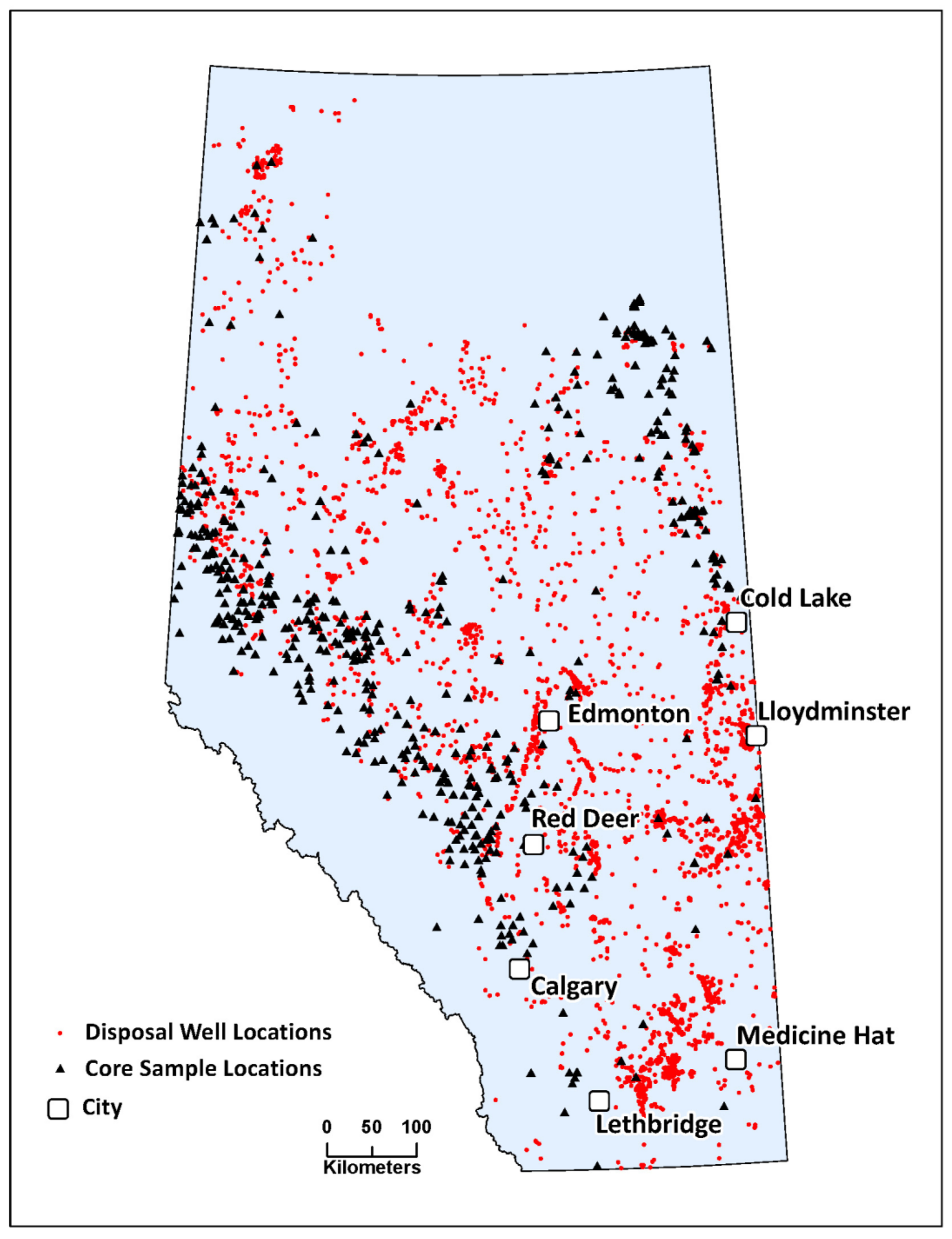
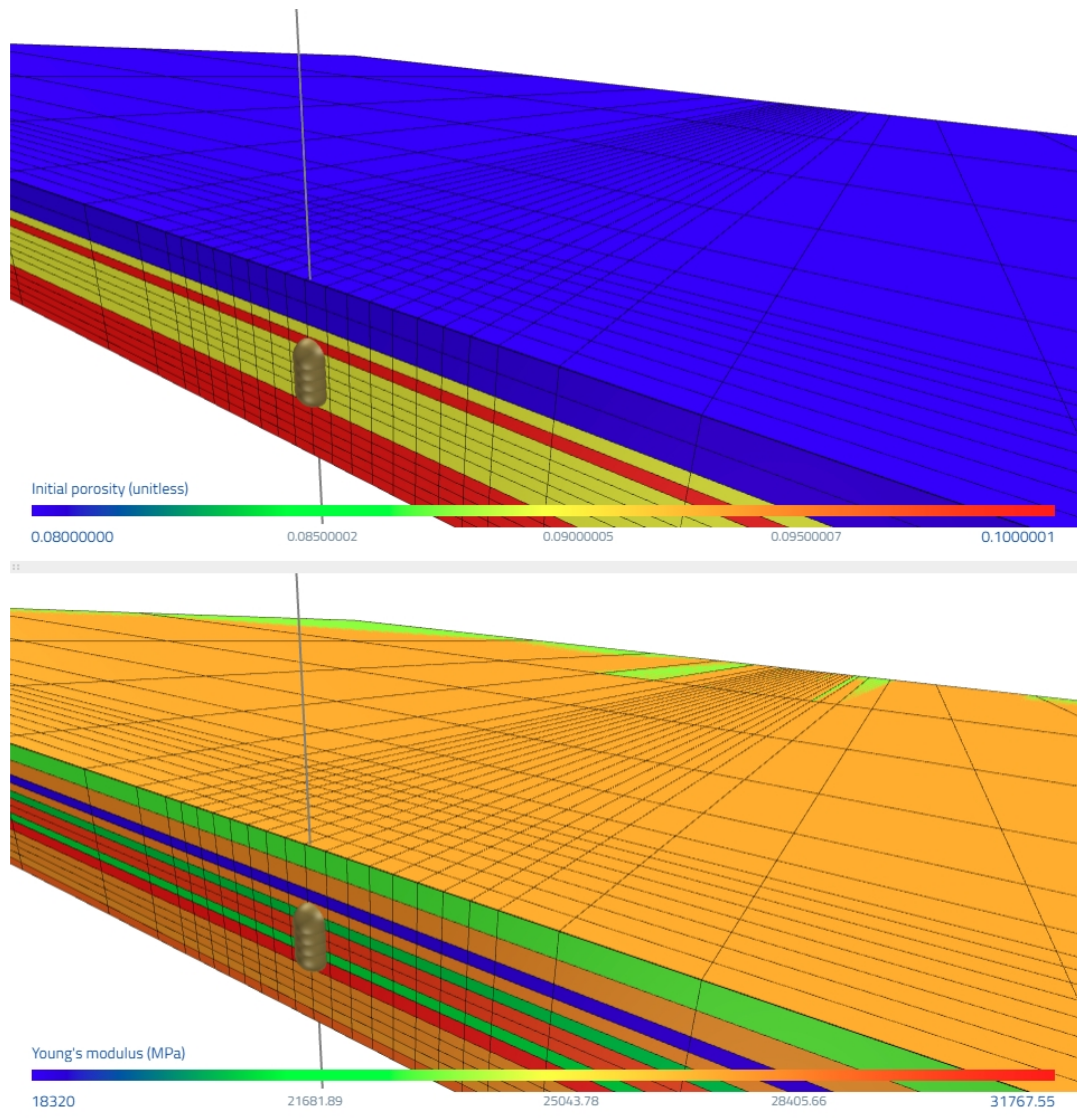
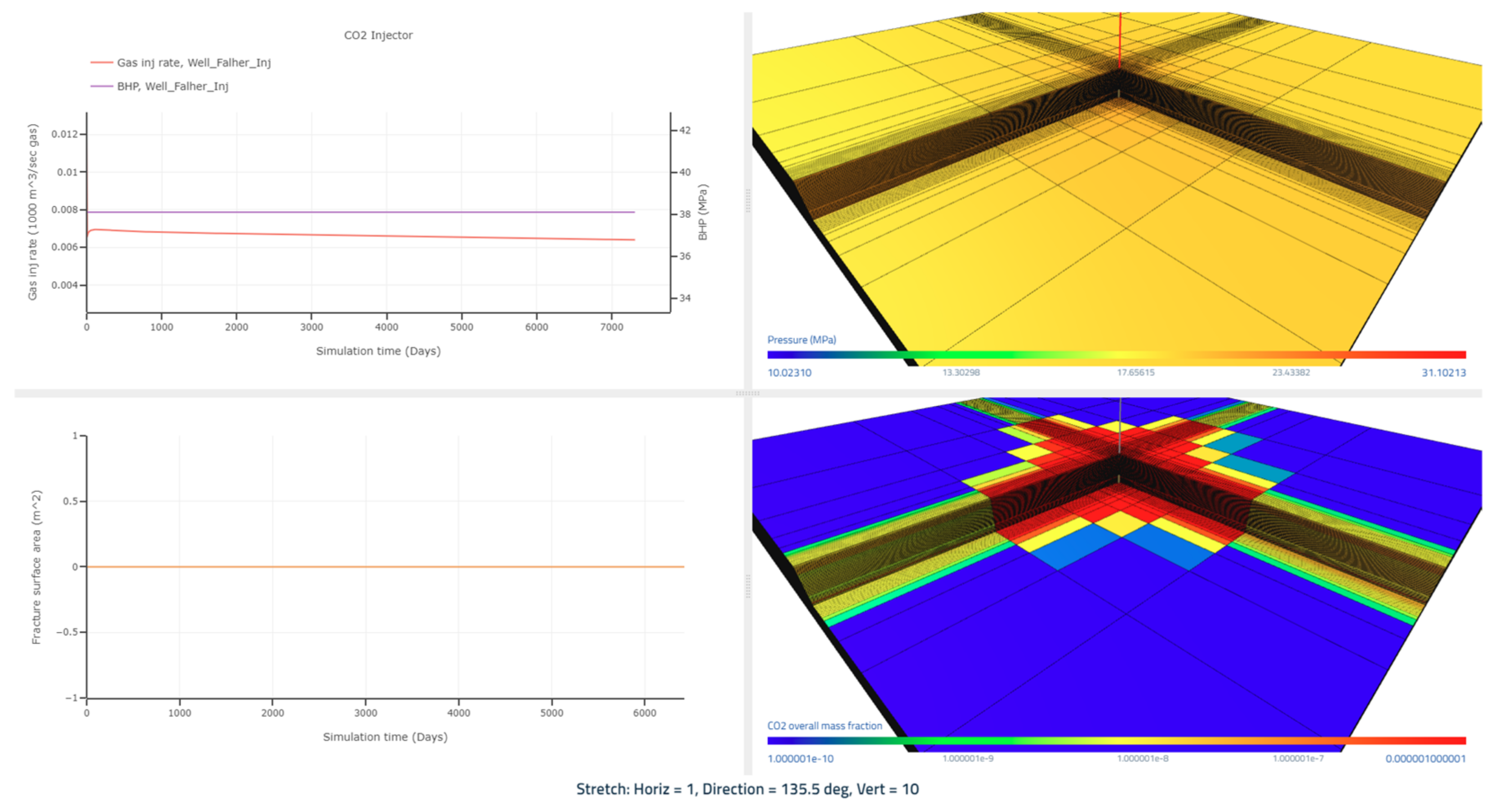
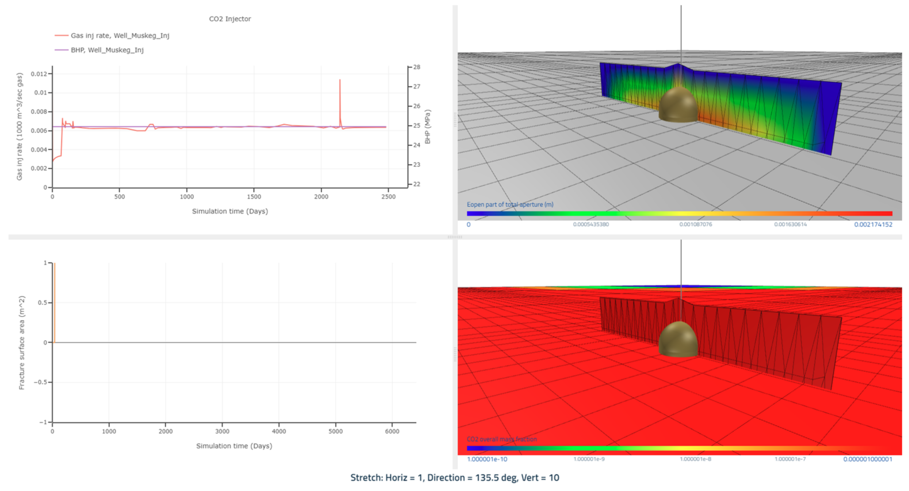
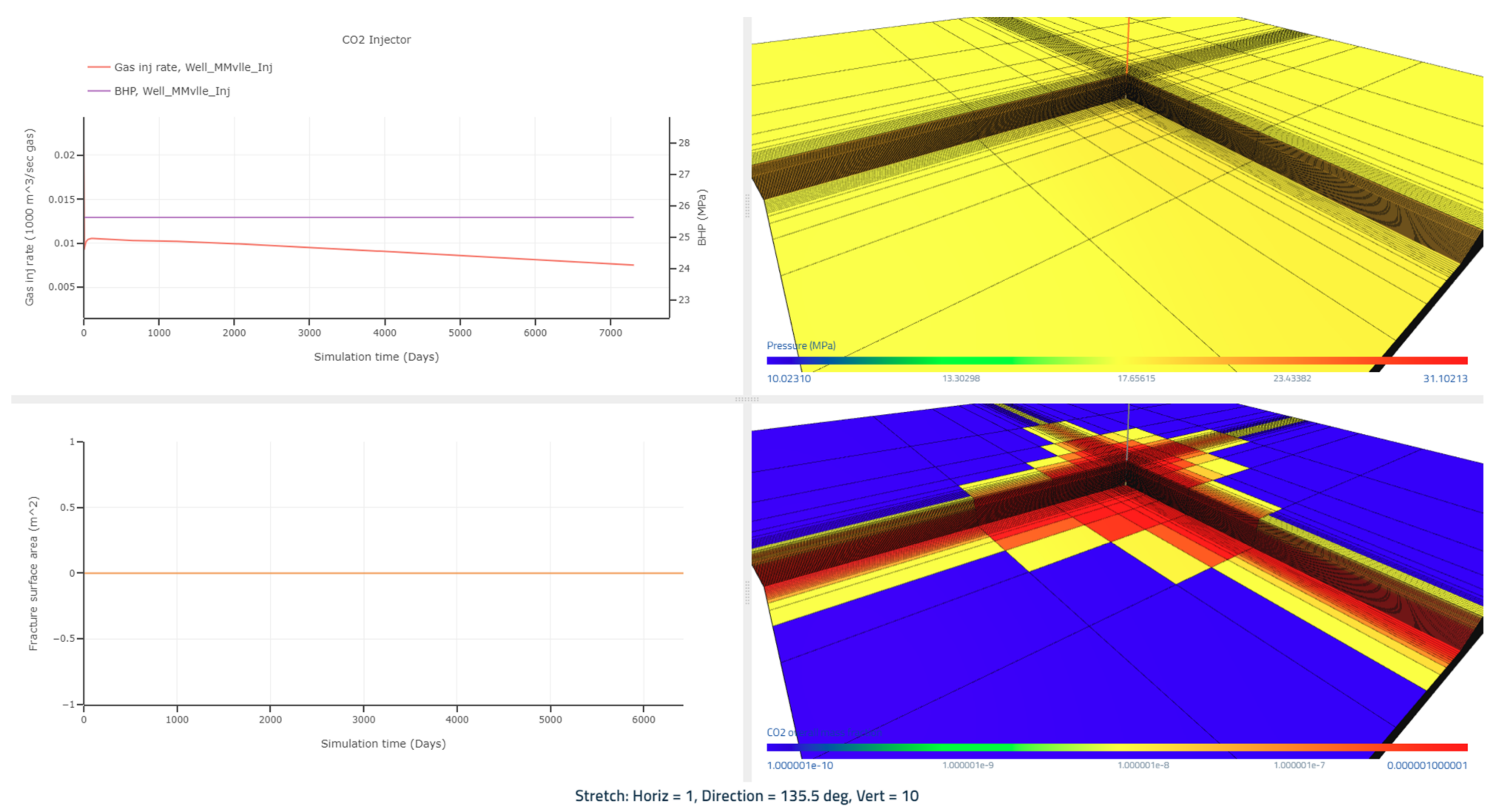
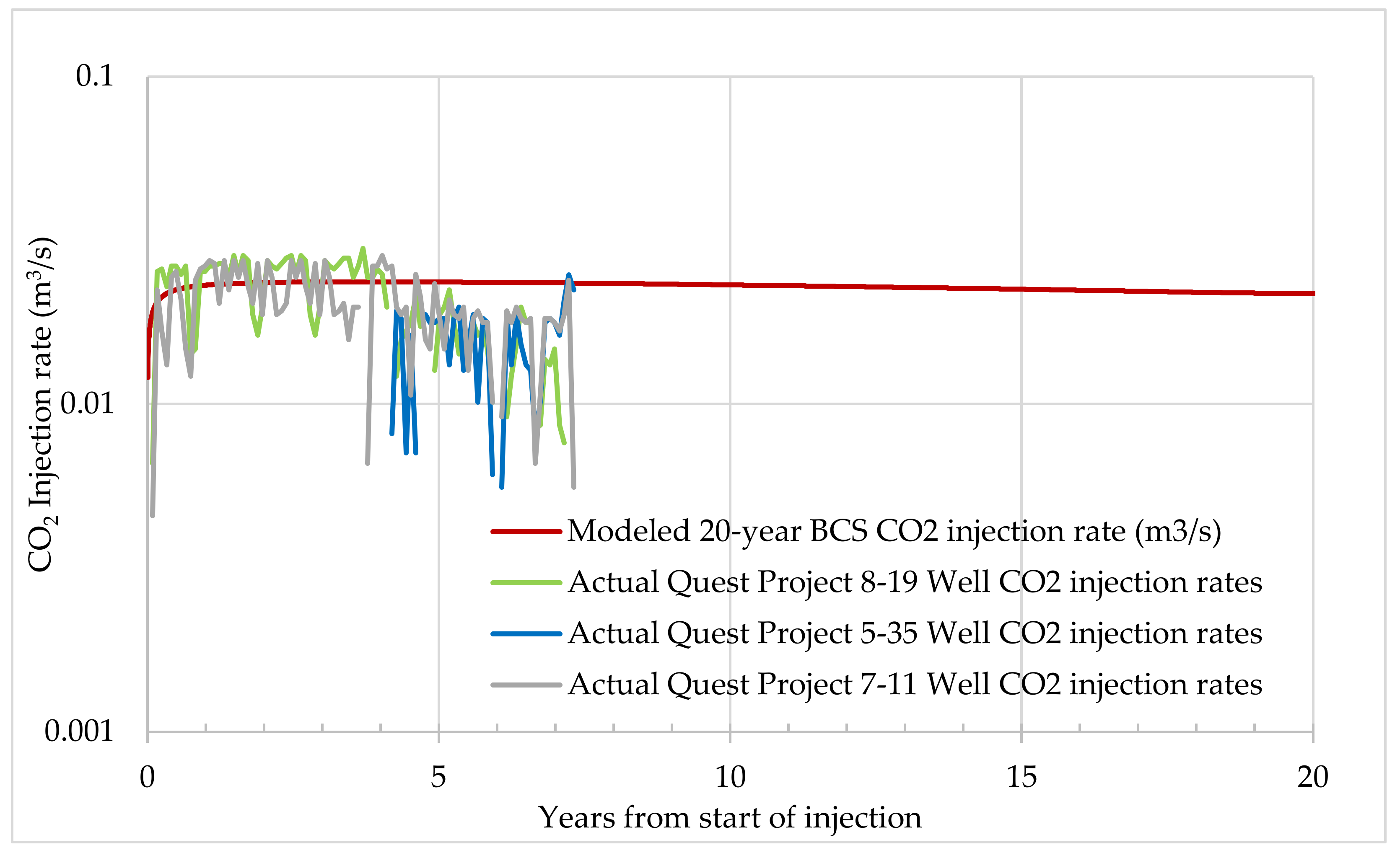
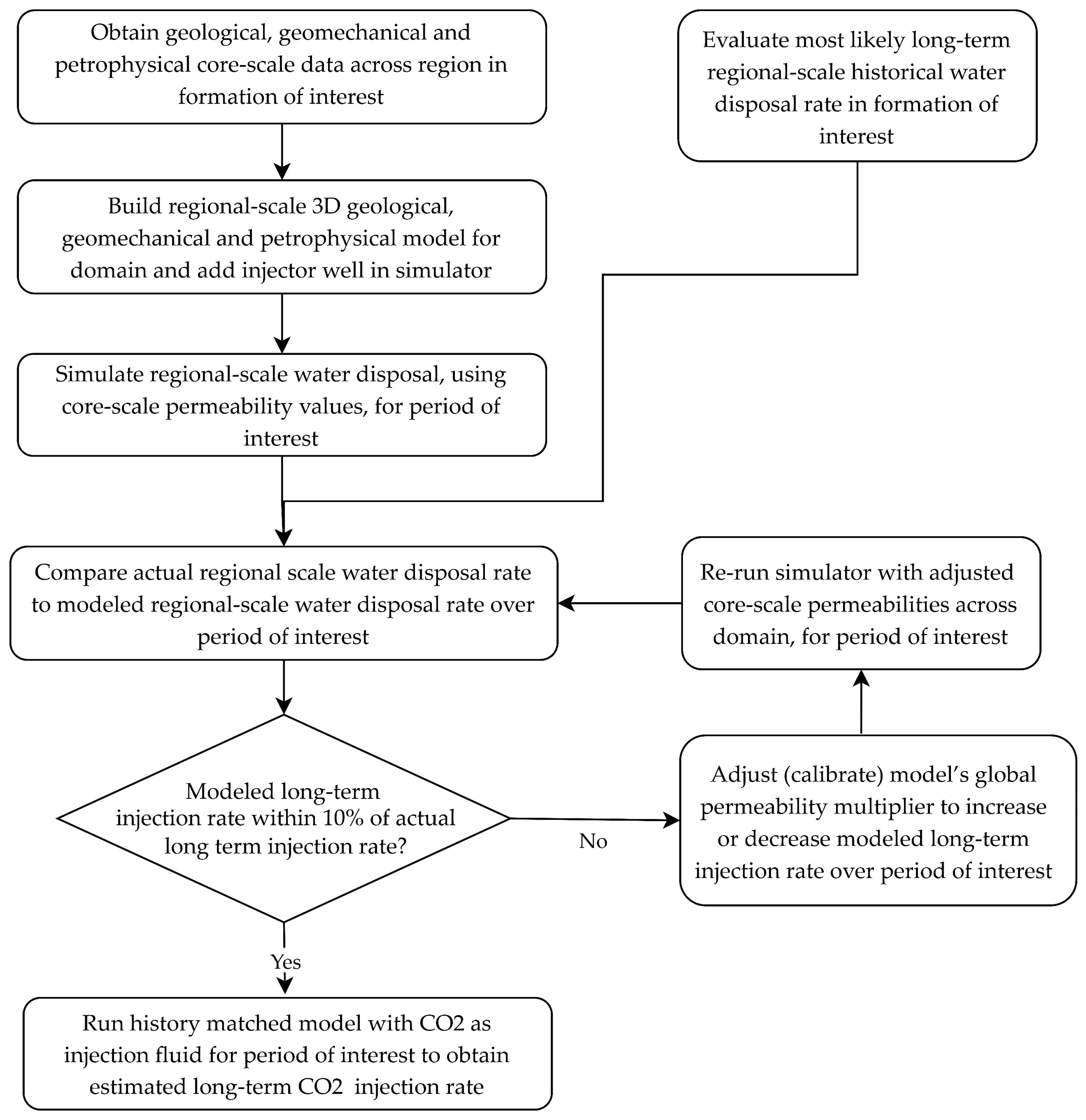
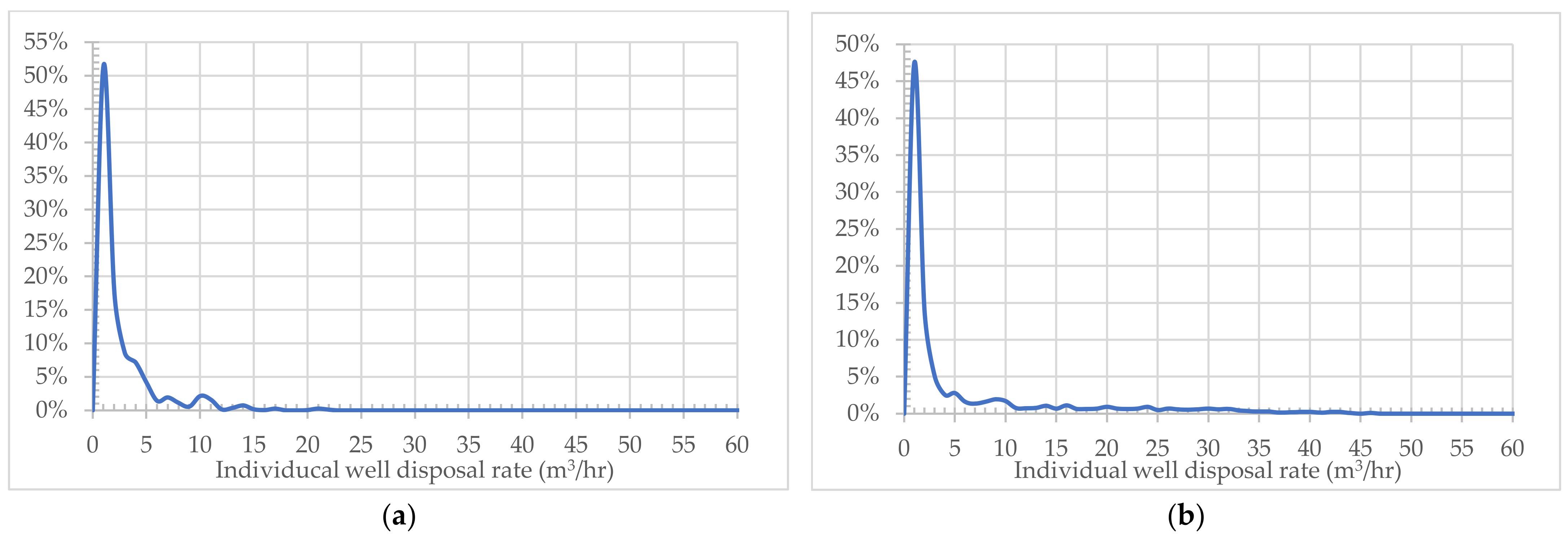
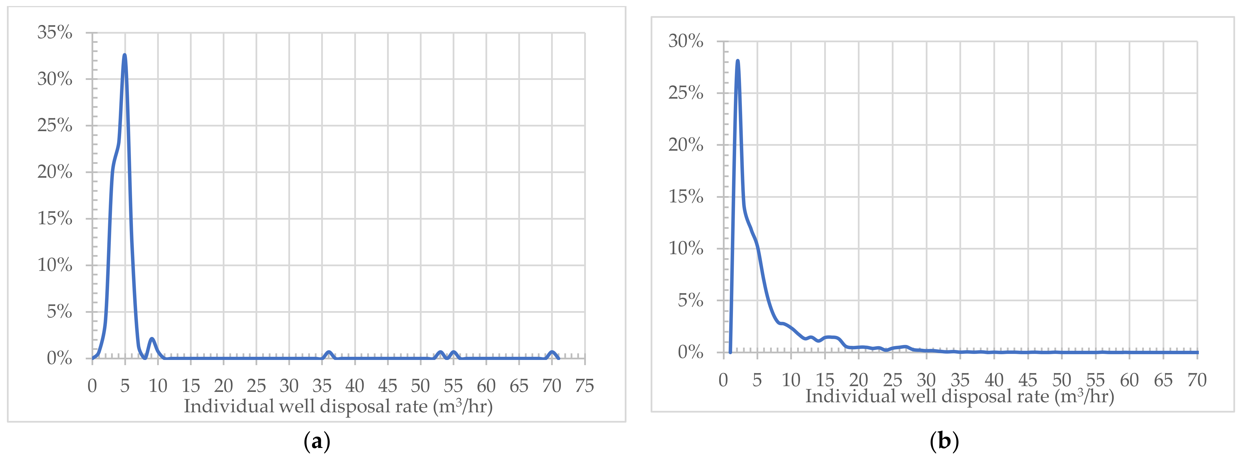
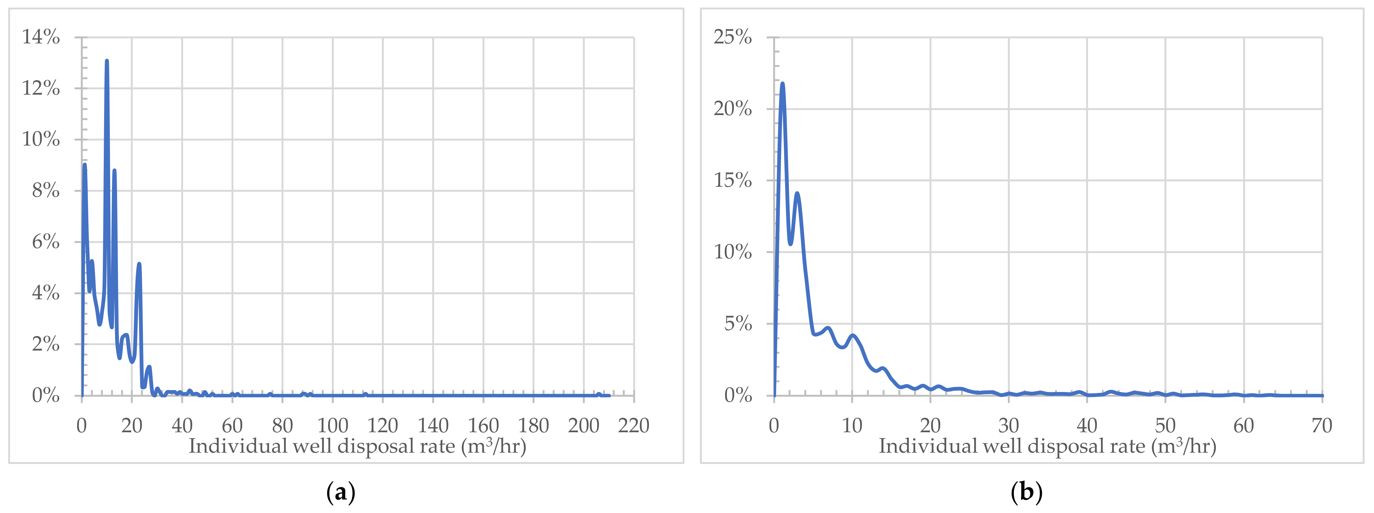
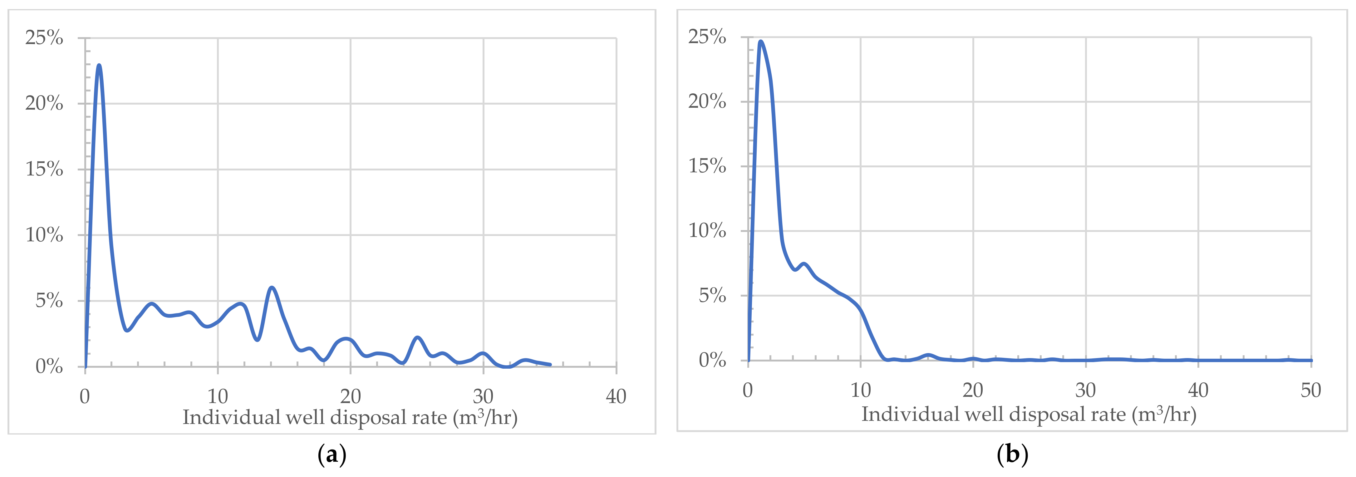
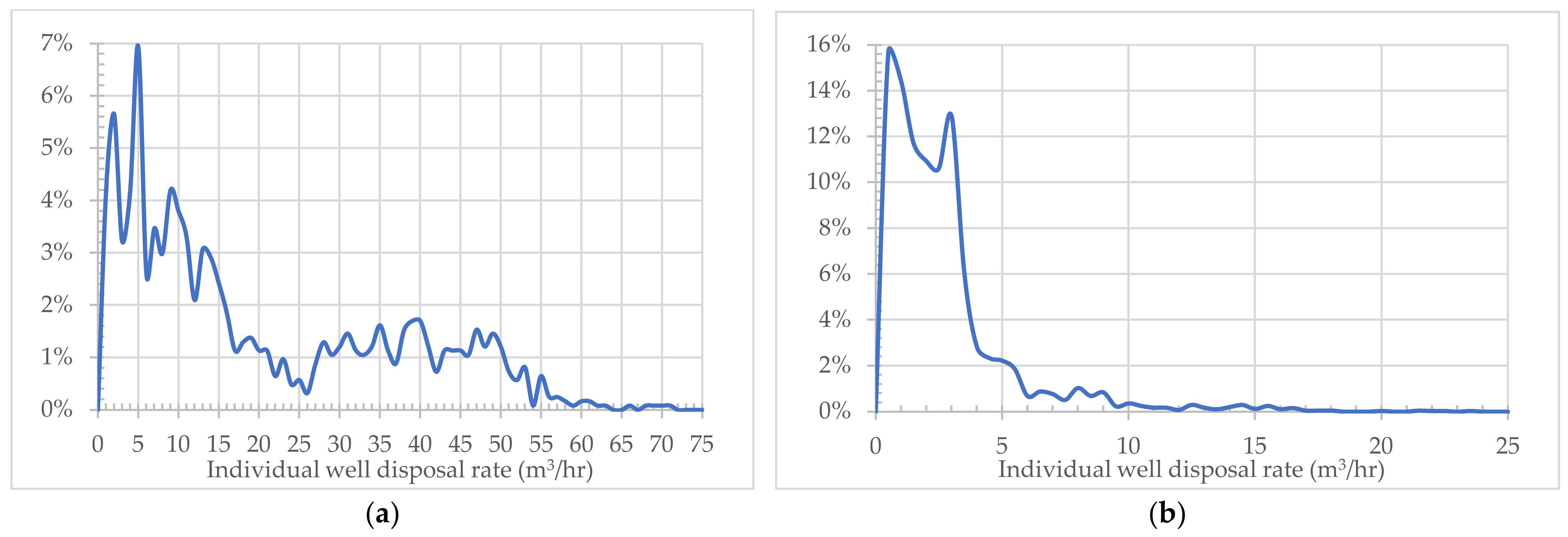
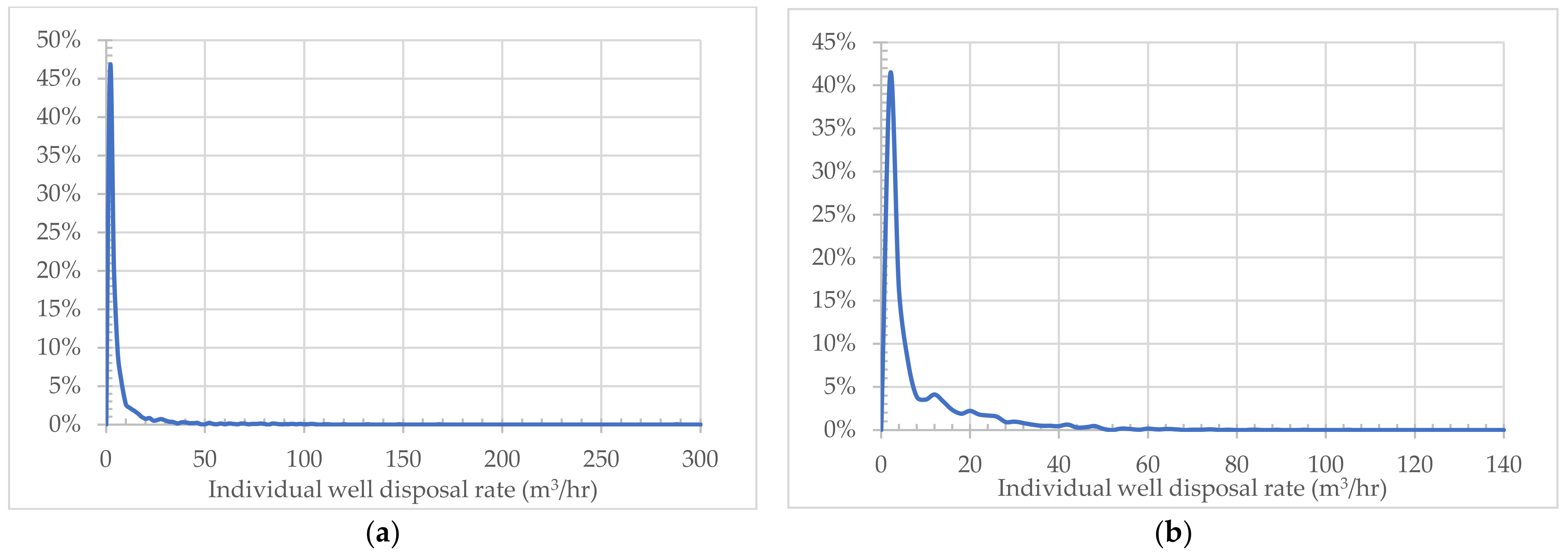
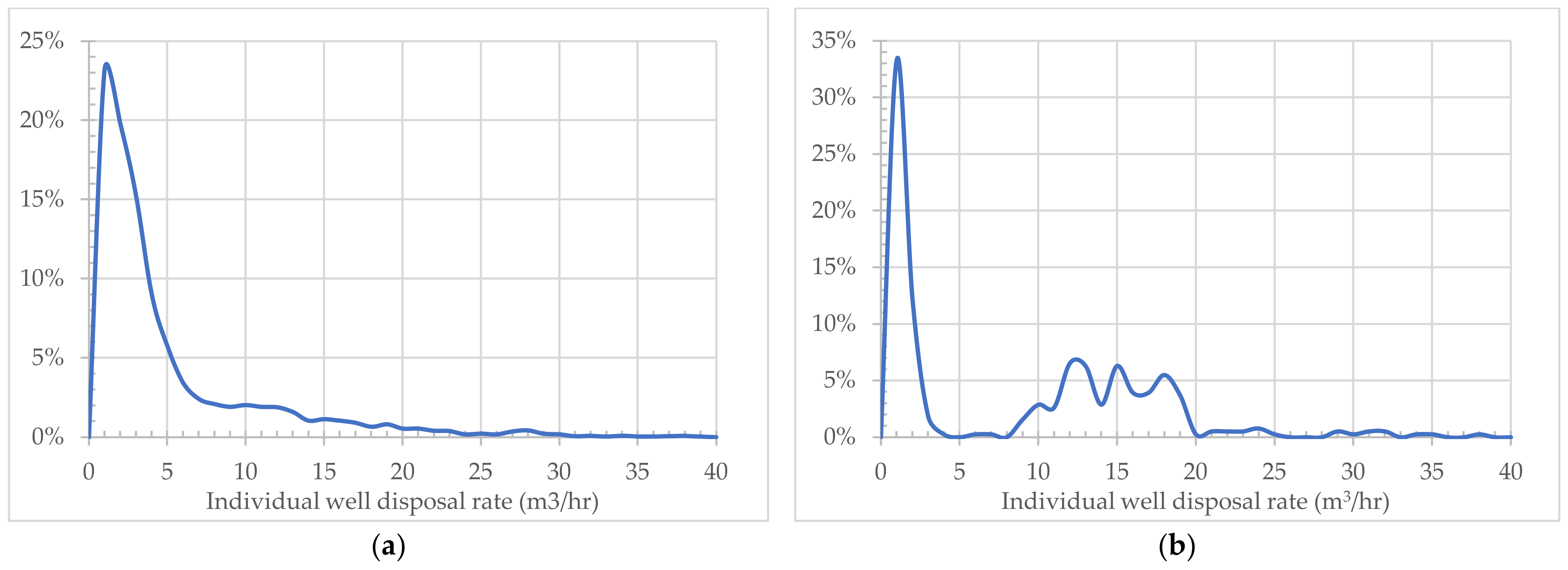
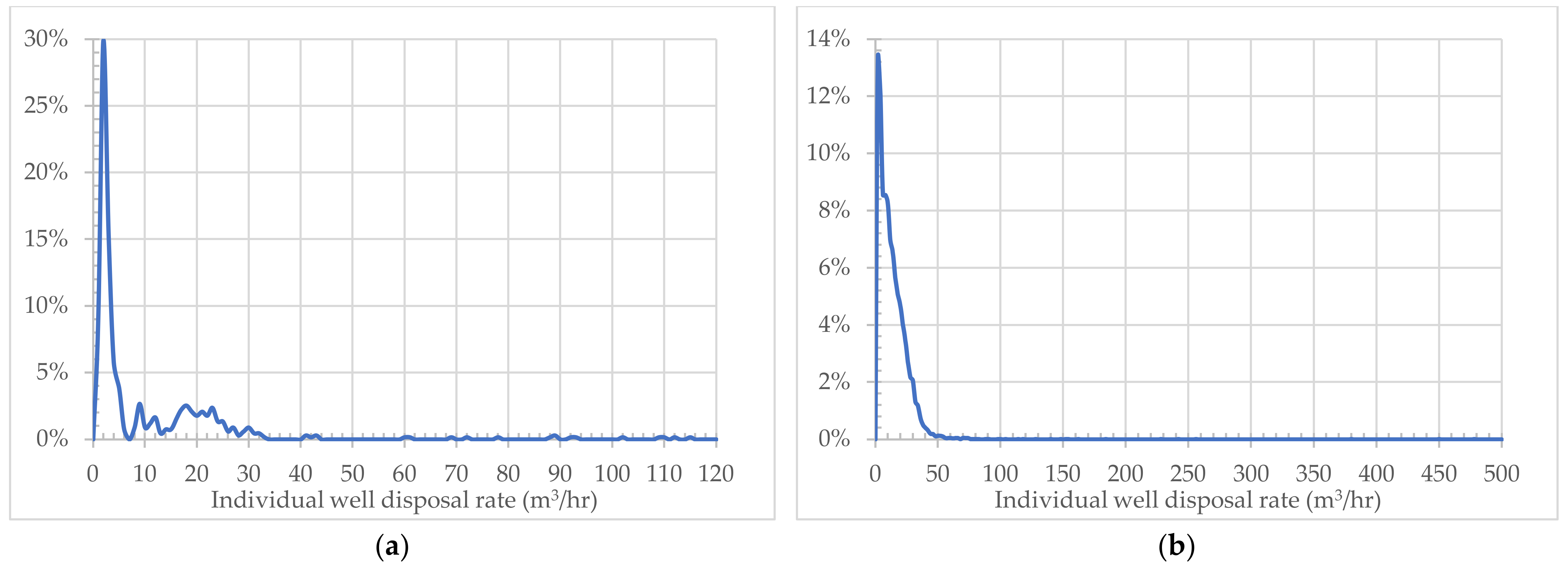
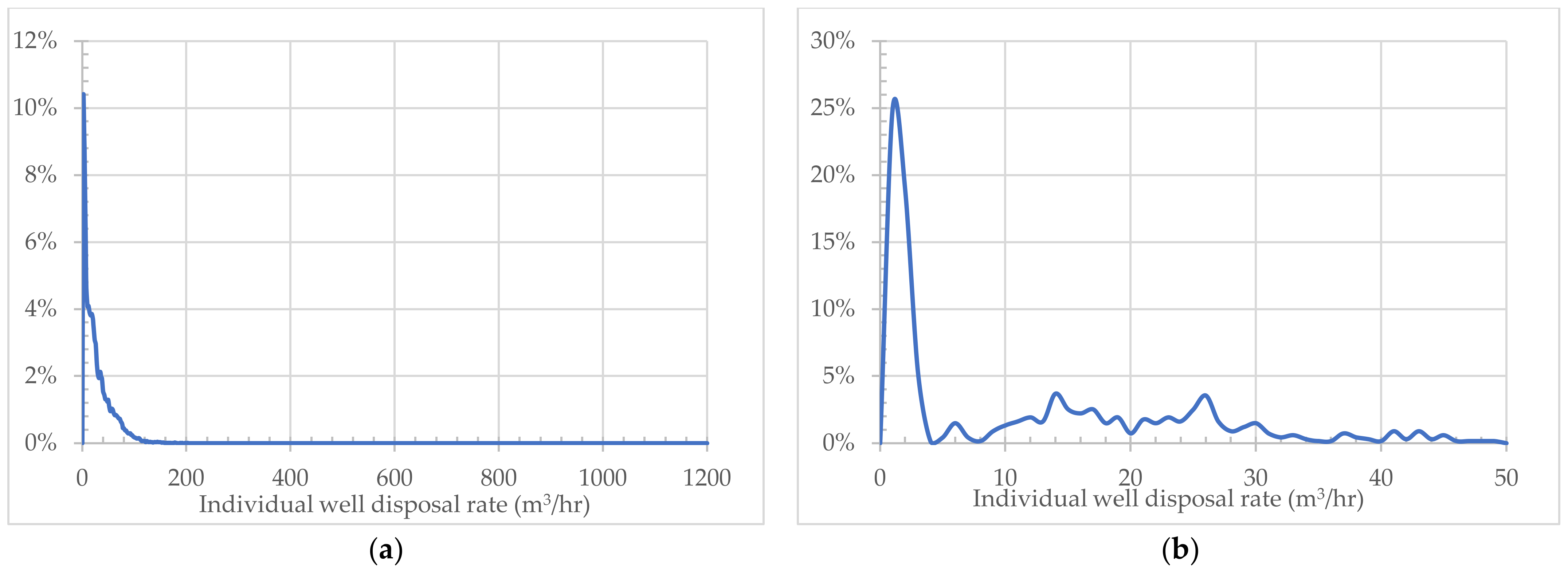
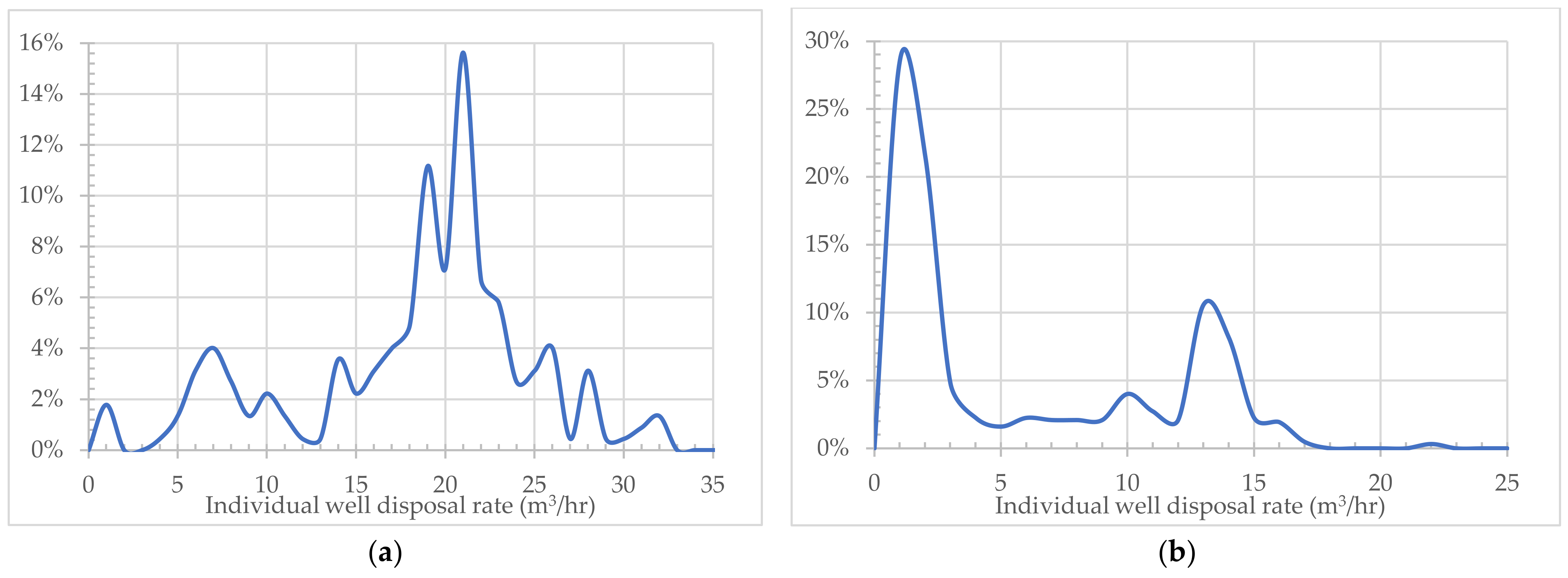
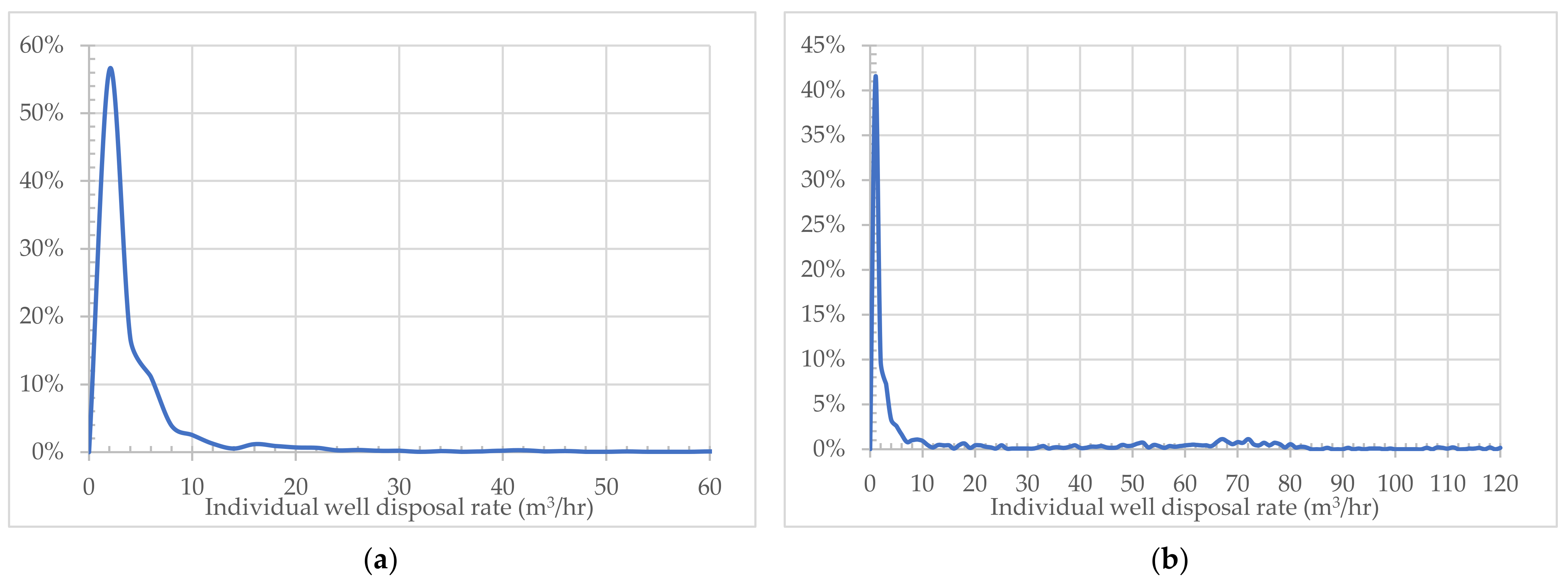
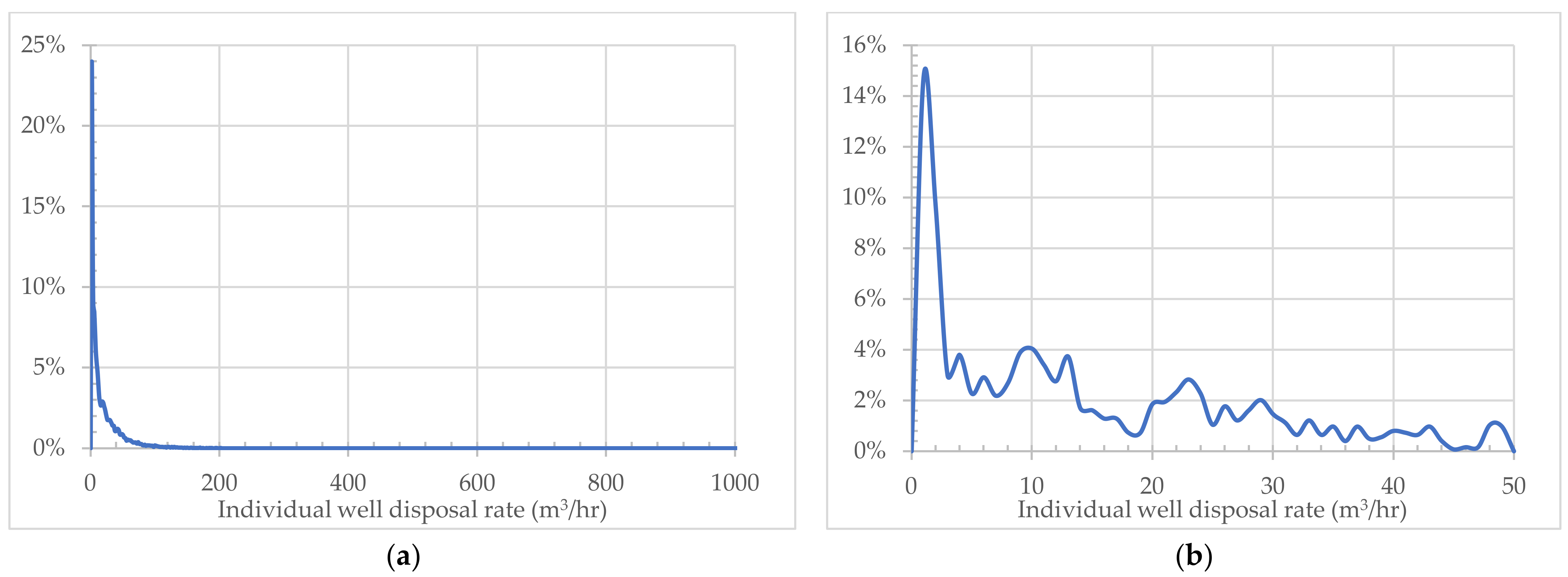
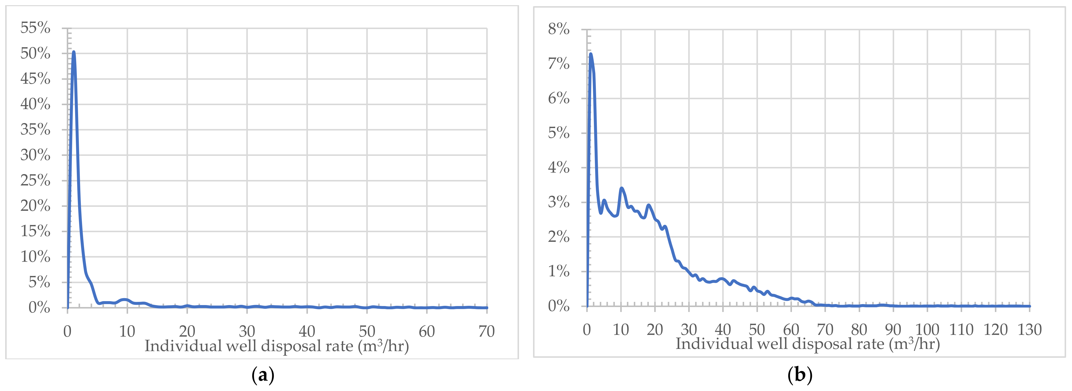
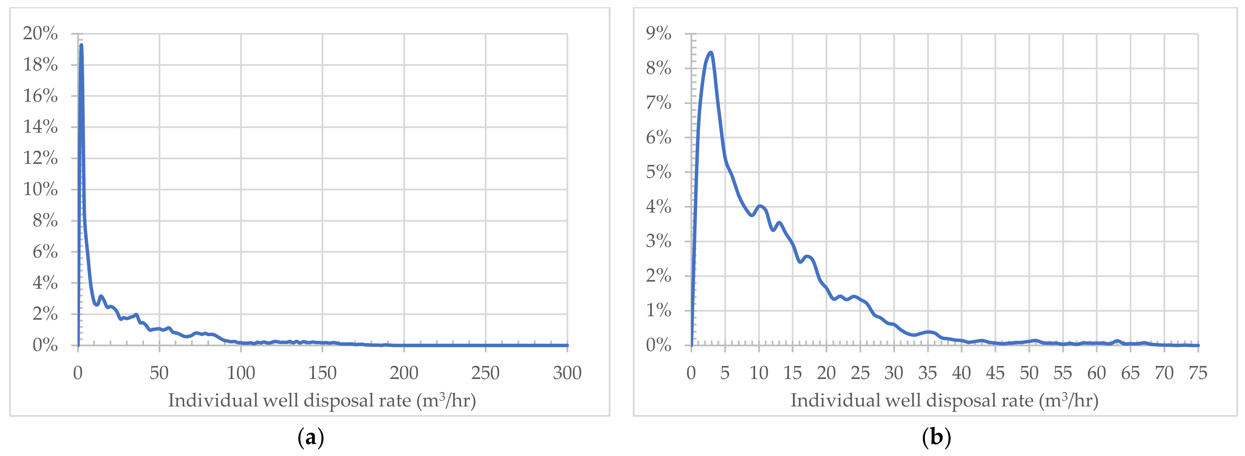
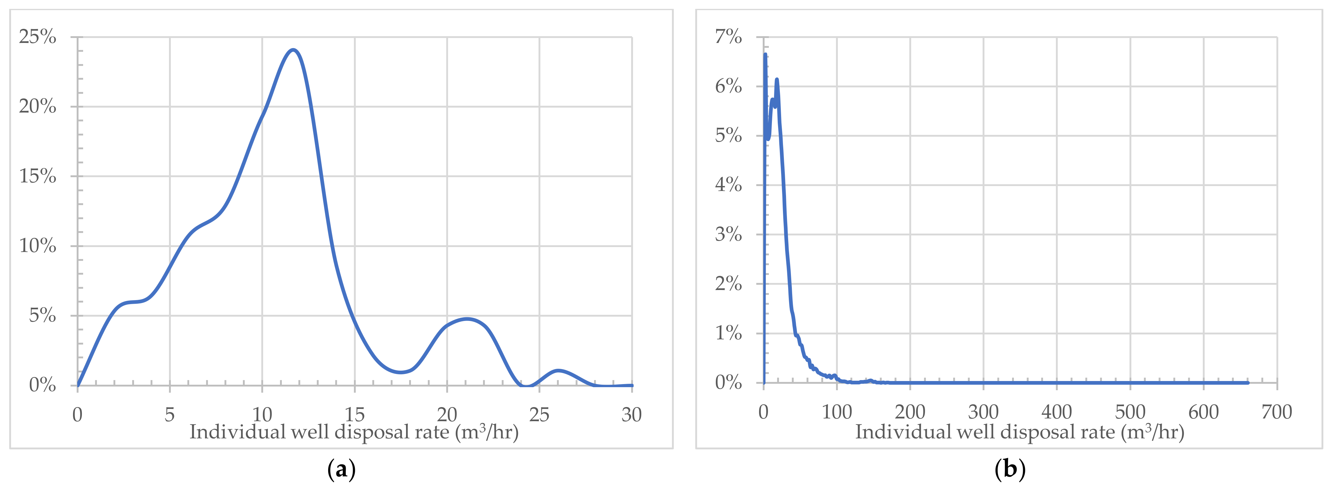
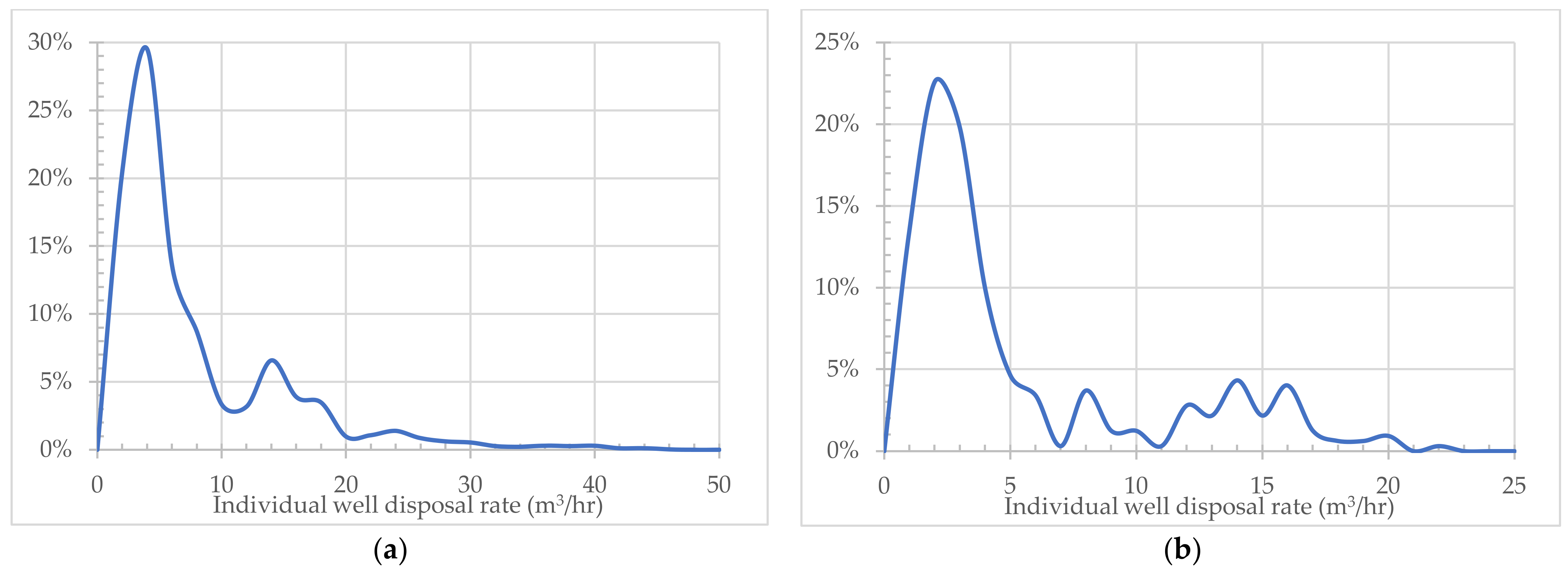
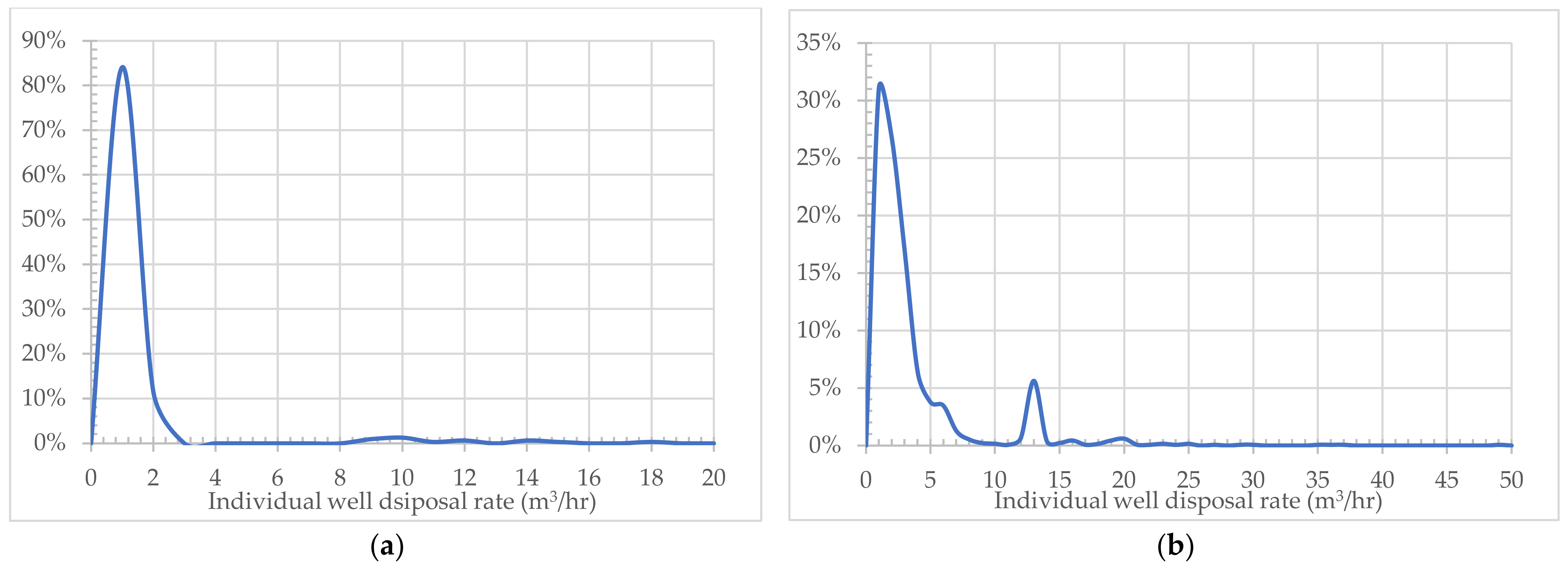
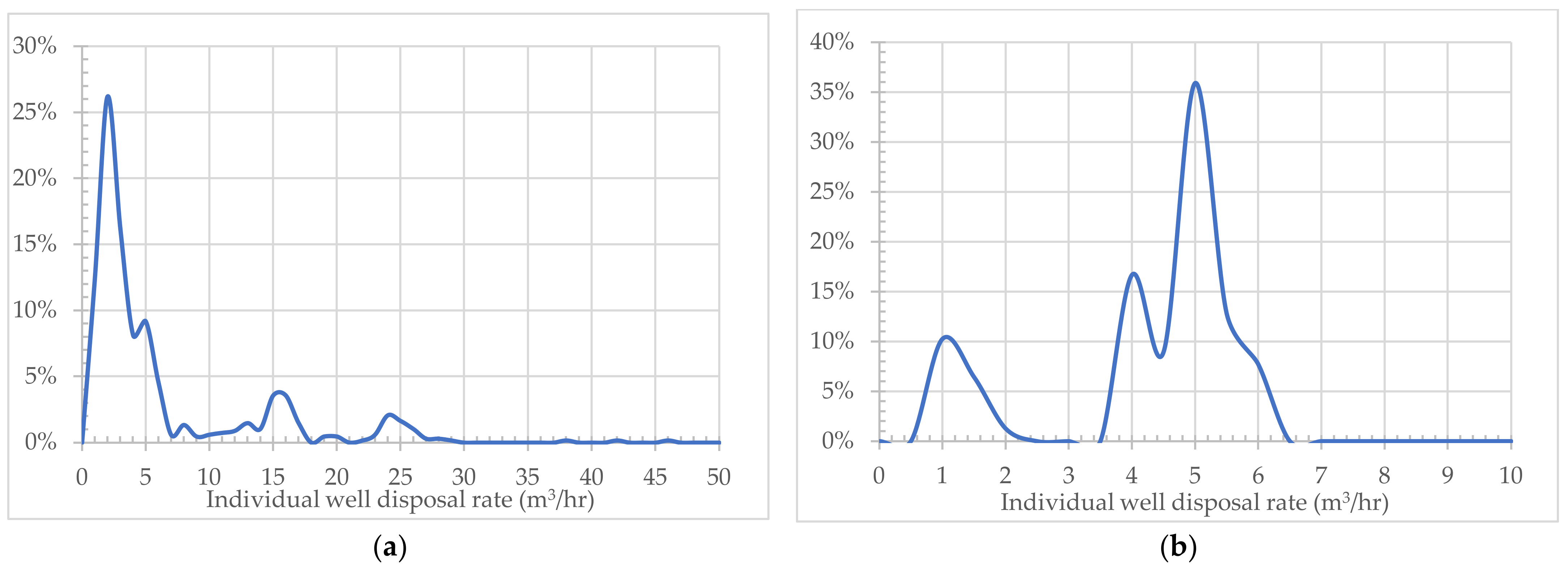
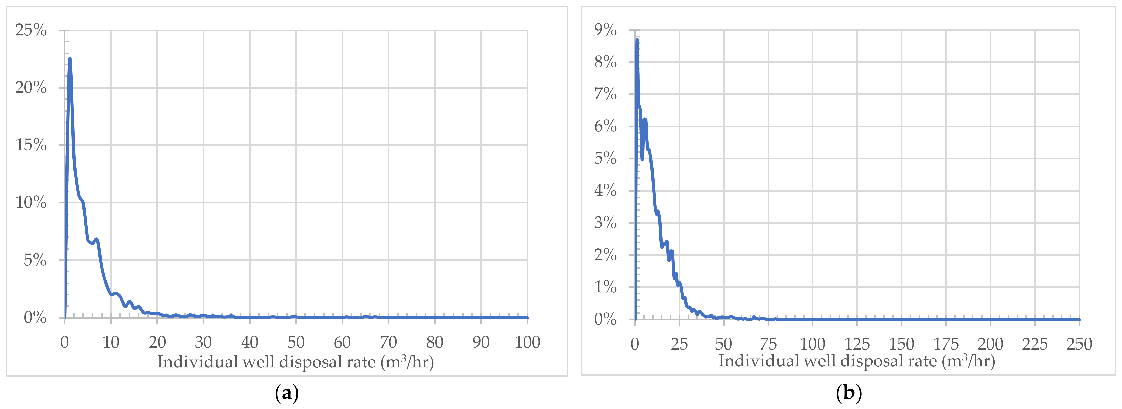
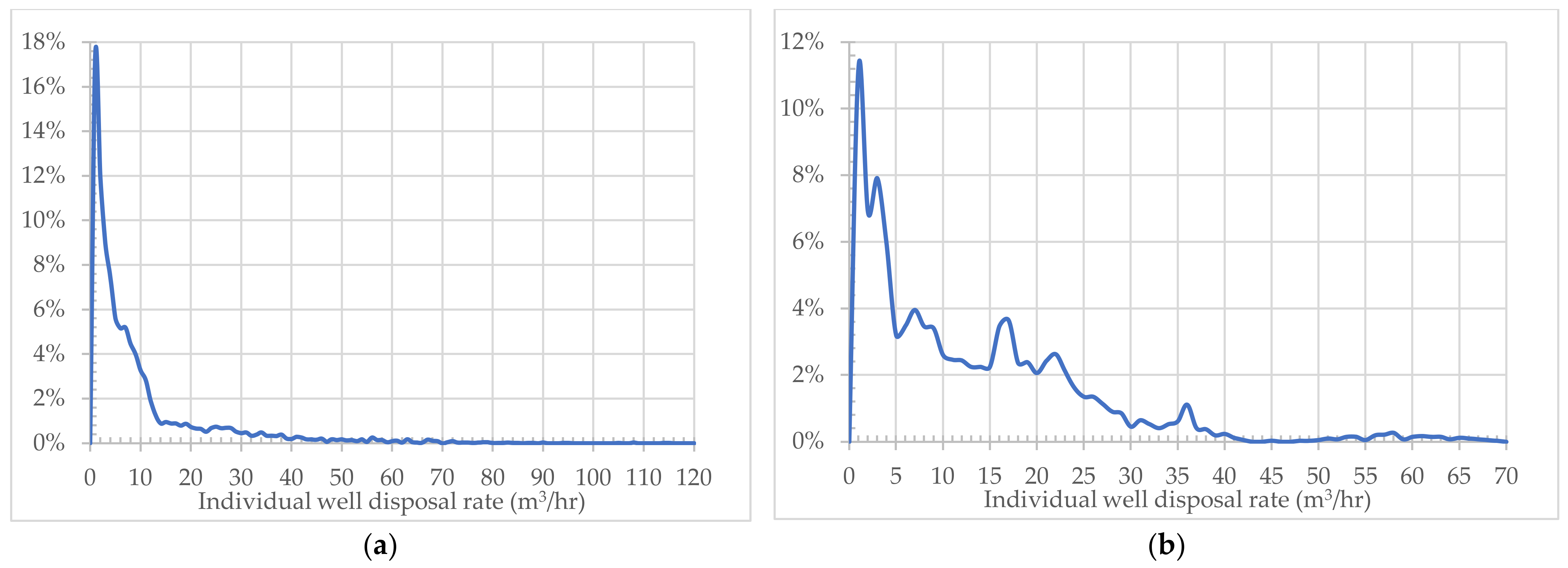
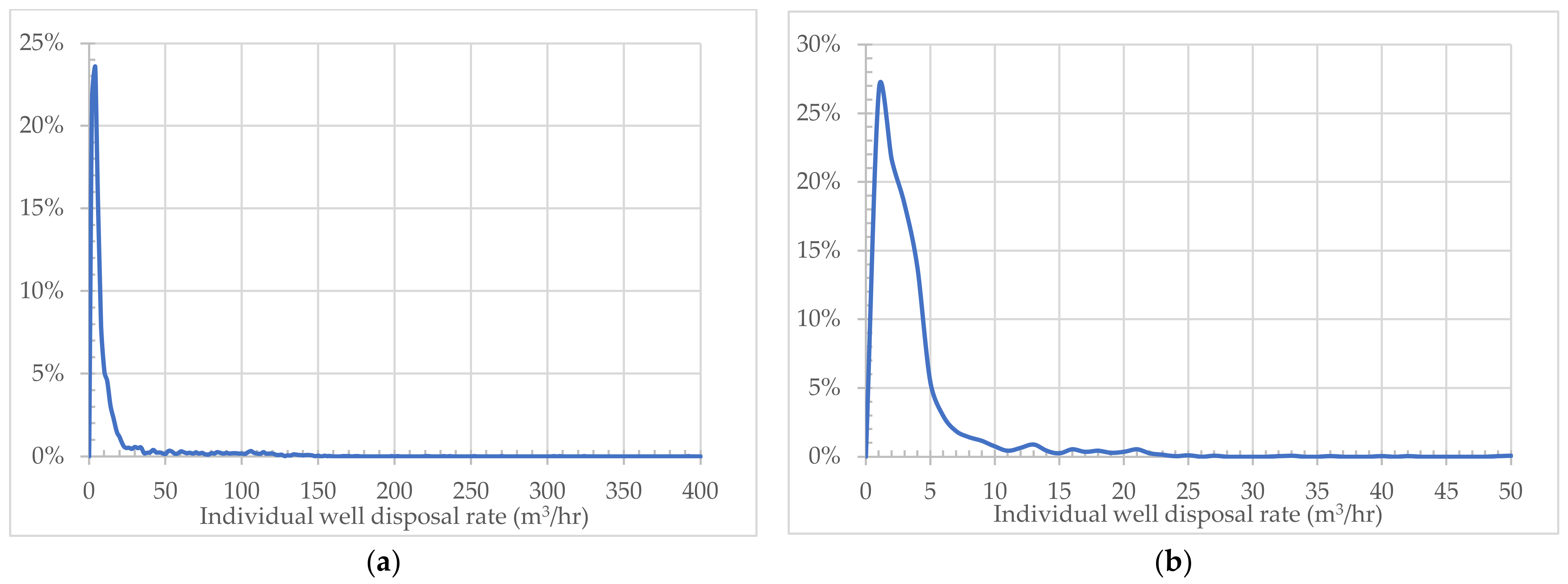
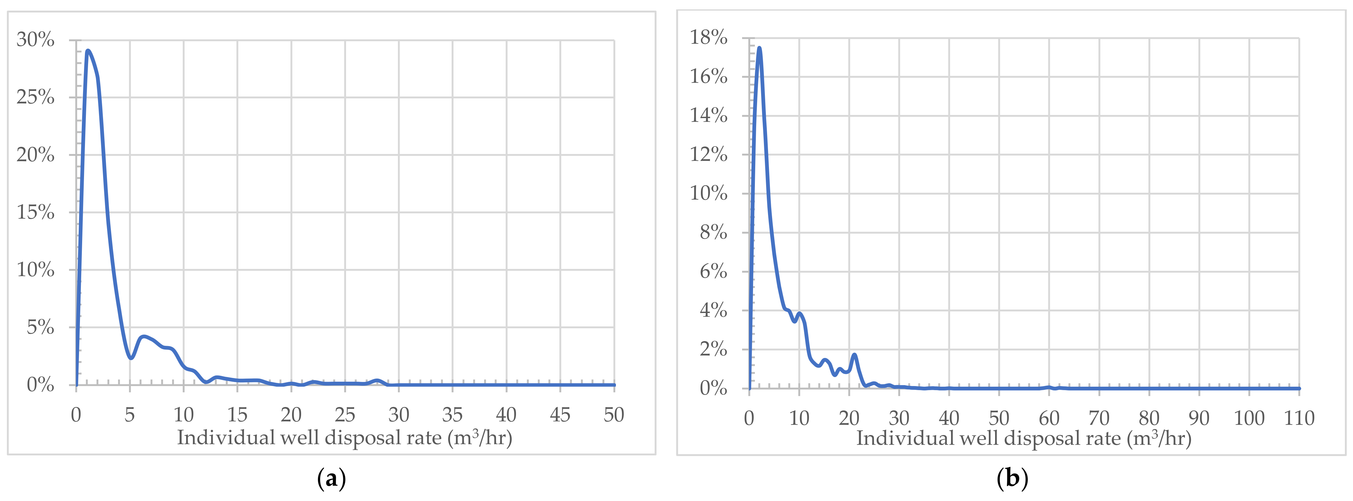
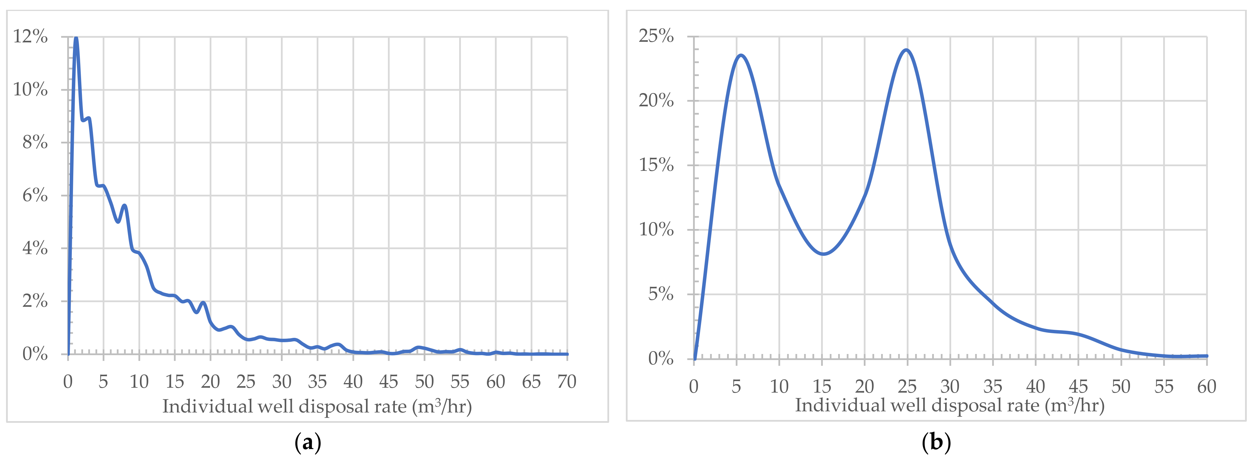
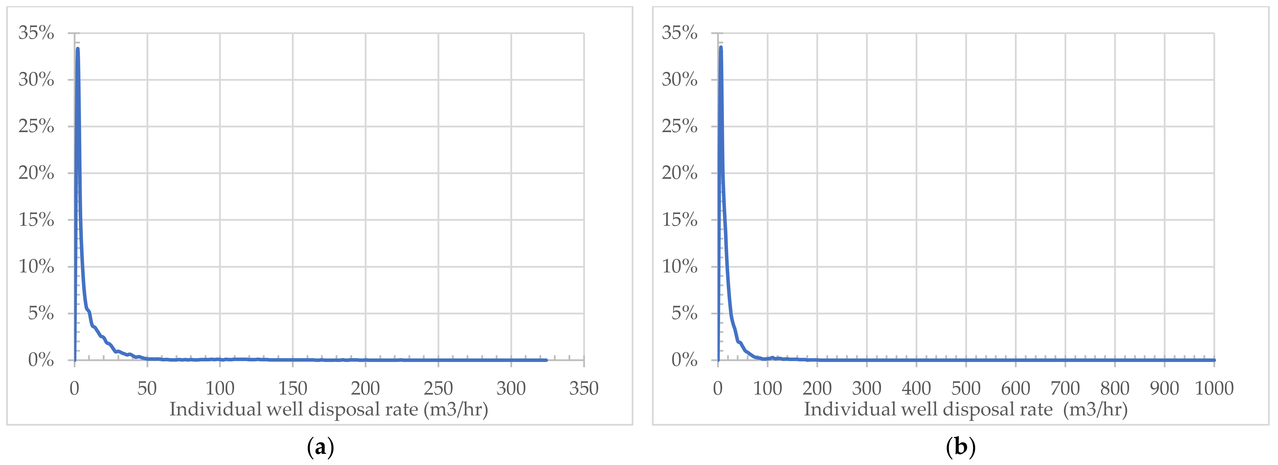
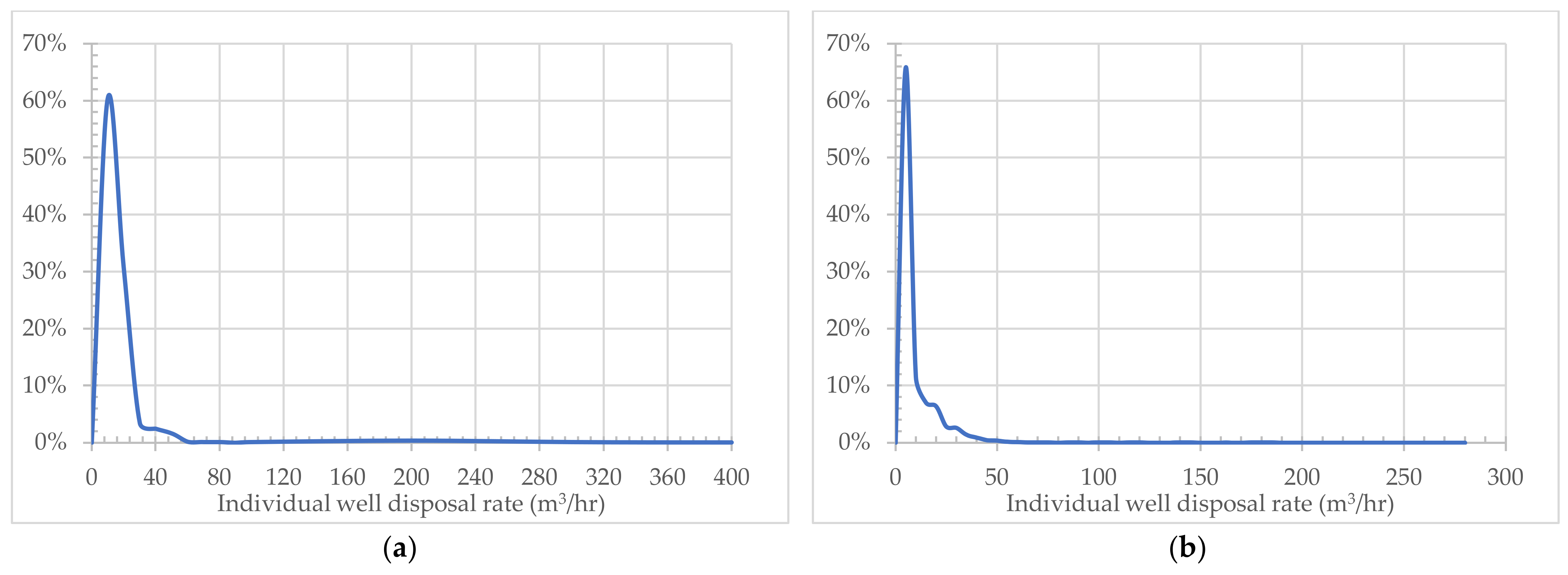
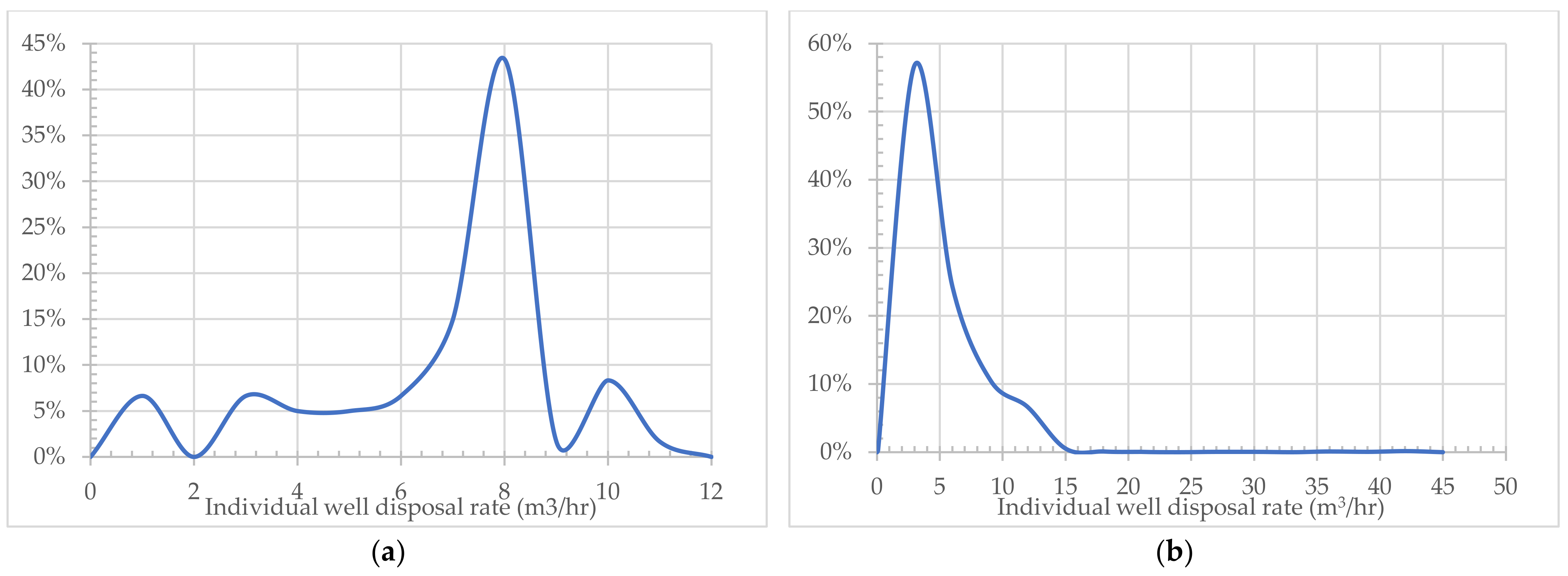
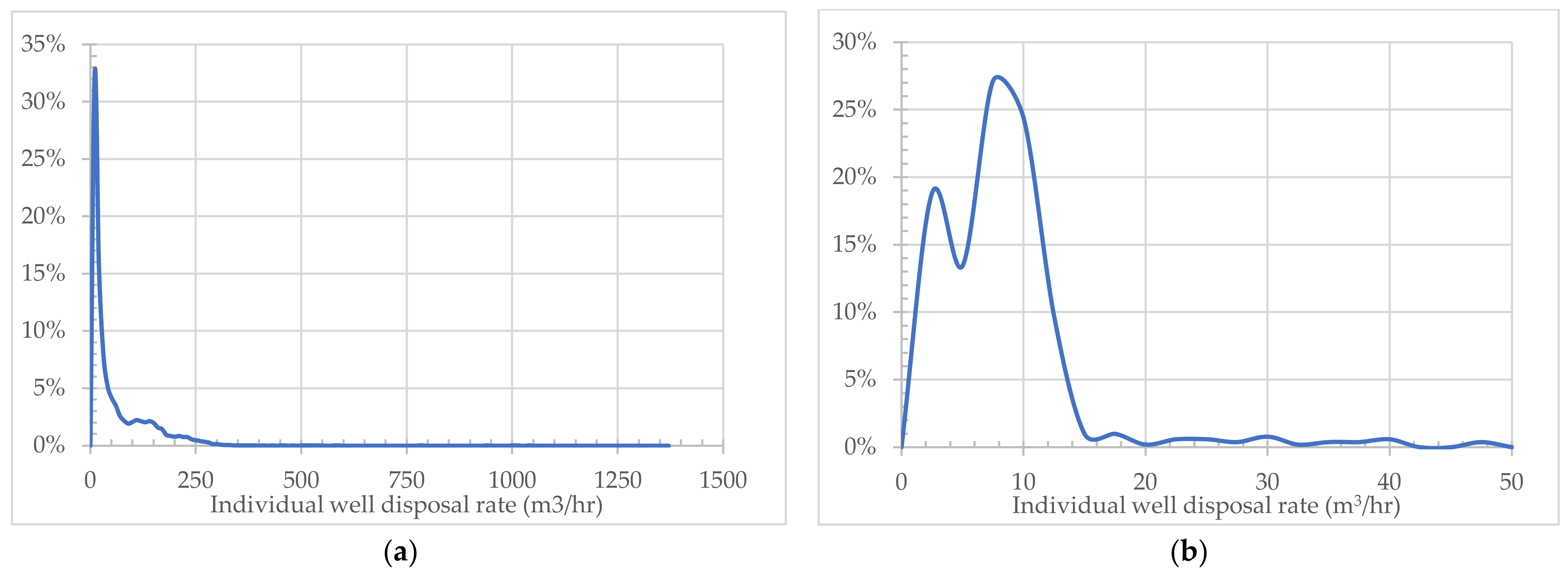
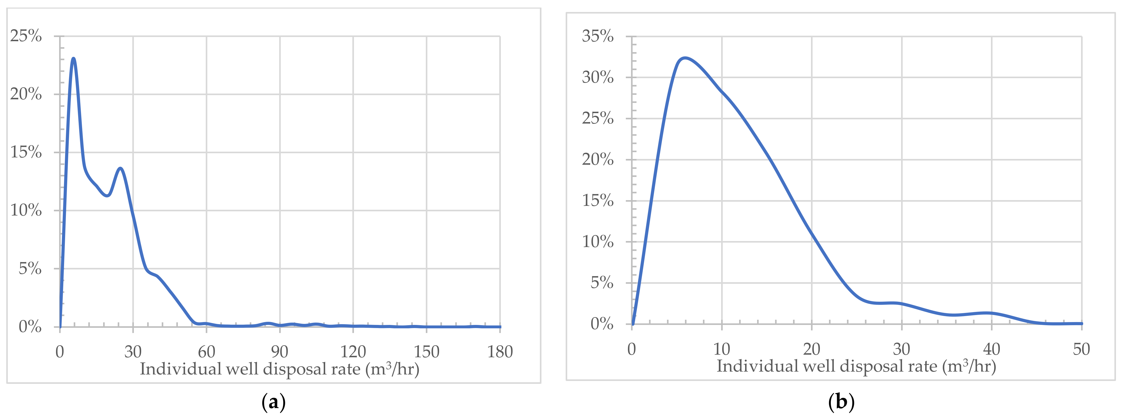
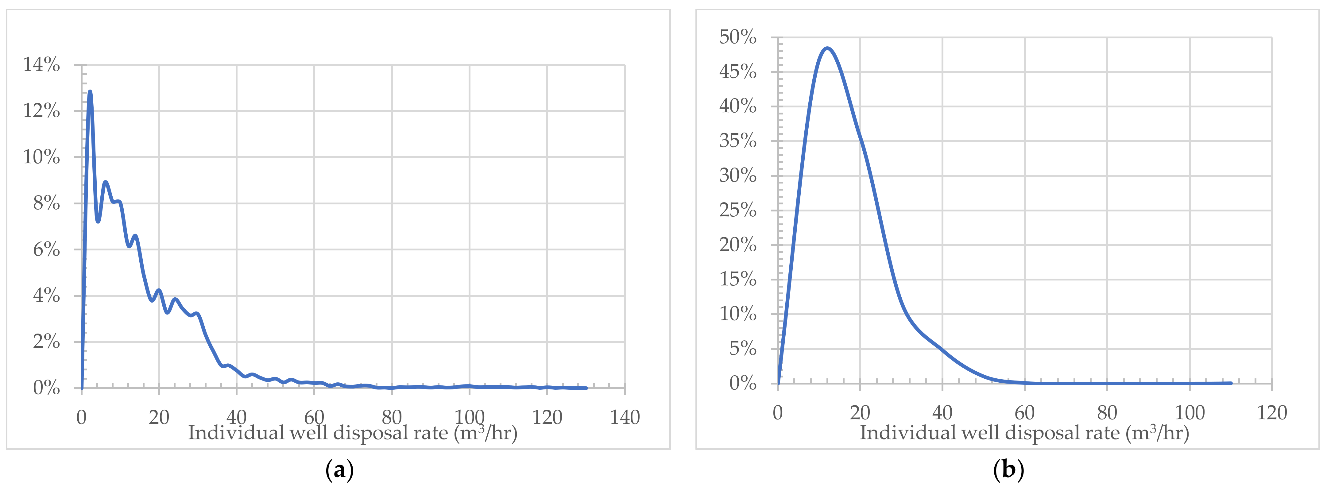
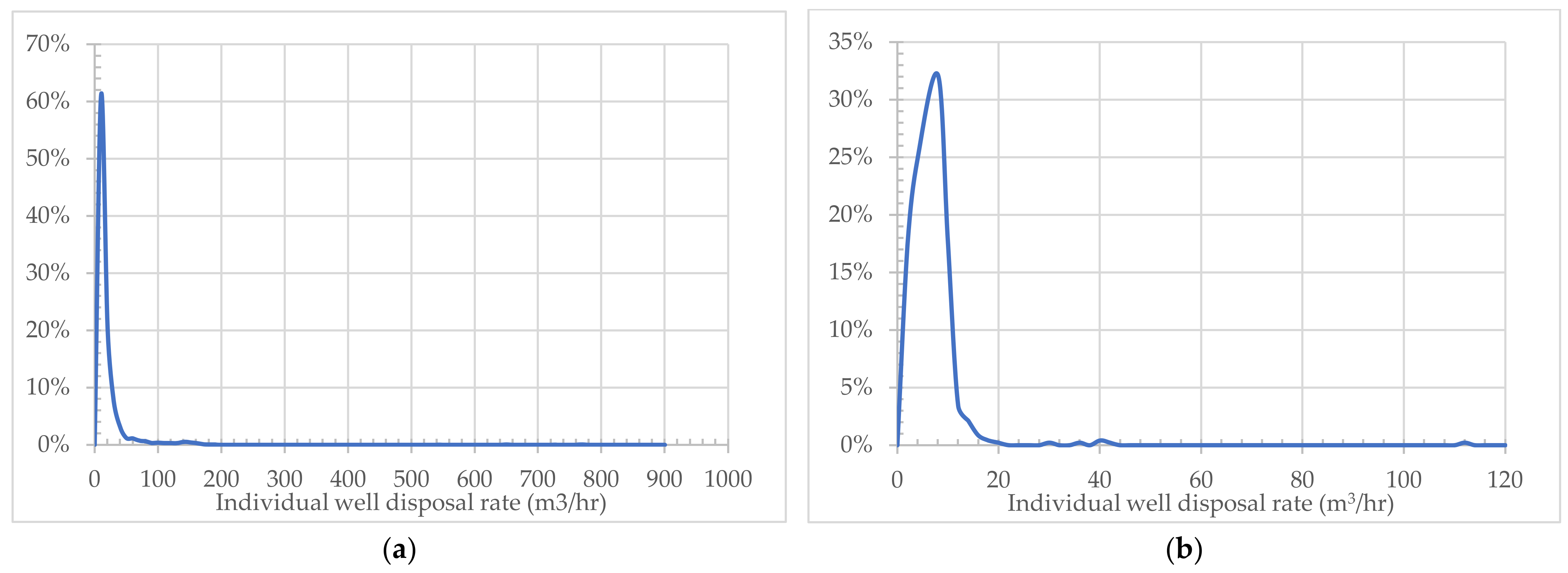
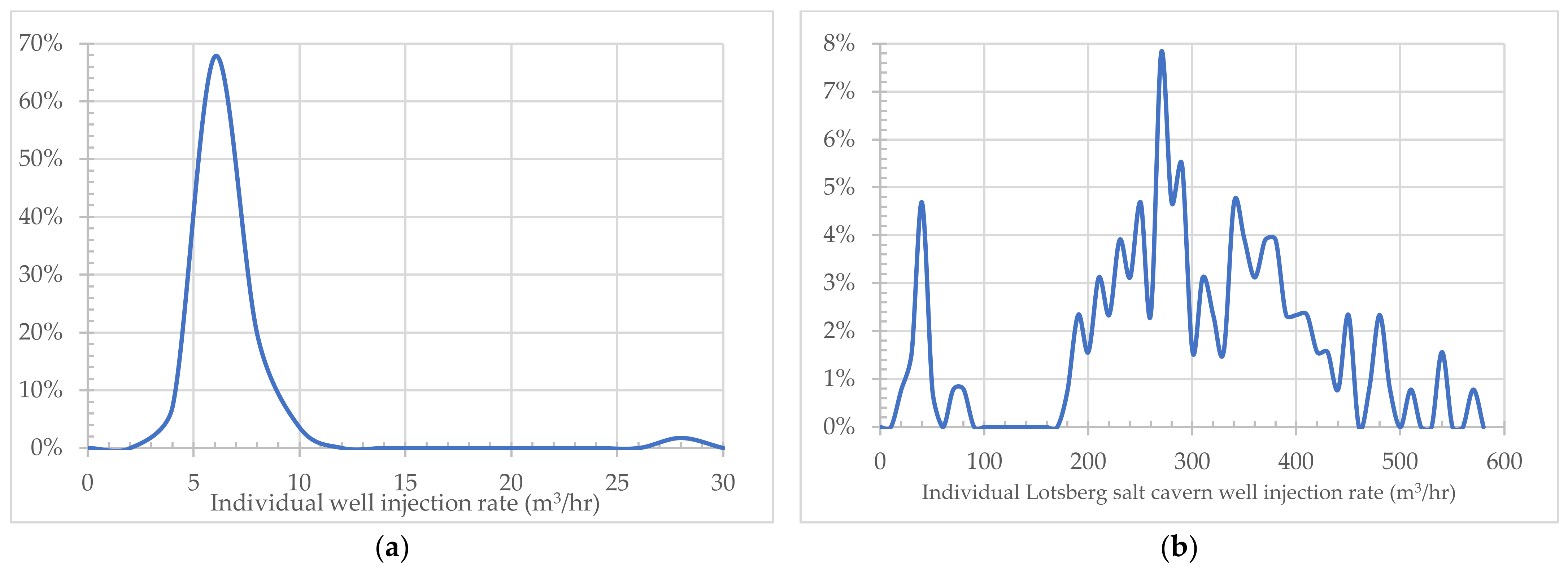
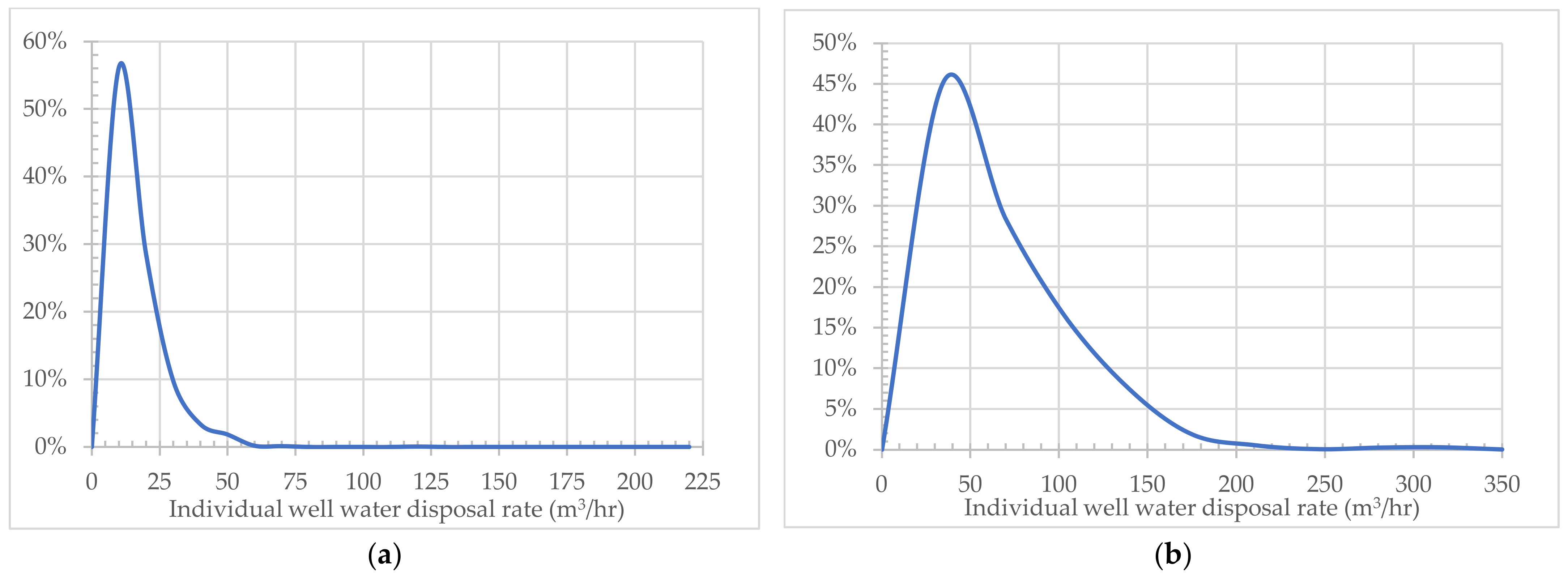
Table 1.
Key recipient formations for all types of fluid injection in the Alberta Basin over the period January 1962 to December 2021. After Samaroo et al. (2022) [13] and used with permission. Detailed production/injection and net fluid balance data for these formations are contained in Samaroo et al. (2022) [13].
| Lithotype and Geologic Formation | Water Injected 1 | Gas Injected 1 | Steam Injected 1 |
|---|---|---|---|
| Paleogene sands (Swan Hills) | 17.1% | 14.0% | 0% |
| Lower Cretaceous sandstones (McMurray, Clearwater, Cardium, Viking, Nikanassin) | 30.6% | 9.8% | 97.9% |
| Jurassic sandstones (Sawtooth) | 11.5% | 15.1% | 0% |
| Triassic carbonates (Charlie Lake, Halfway) | 0.4% | 1.0% | 0% |
| Triassic siltstones (Montney, Doig) | 0.3% | 0.6% | 0% |
| Permian sandstones (Belloy) | 0.2% | 0% | 0% |
| Carboniferous carbonates (Banff, Debolt, Elkton, Livingston, Turner Valley) | 0.7% | 1.8% | 0% |
| Devonian carbonates (Arcs, Grosmont, Keg River, Leduc, Muskeg, Nisku, Slave Point, Wabamun, Winterburn) | 29.2% | 43.3% | 1.4% |
| Devonian sandstones (Granite Wash, Gilwood) | 4.1% | 0.6% | 0% |
| Cambrian sandstones (Basal Sandstone Unit) | 0.3% | 0% | 0.8% |
| Total volumes injected in above-listed formations | 23.8 km3 | 596.7 km3 | 3.41 km3 |
| Total fluid volumes injected into all formations in the Alberta Basin | 25.2 km3 | 692.2 km3 | 3.41 km3 |
1 Totals may not add to 100% due to rounding. Fluid volumes are reported in cubic kilometers (i.e., km3 = cubic kilometer = 109 m3), measured at surface conditions. Steam volumes reported in cold-water equivalent volume.
Table 2.
Stratigraphic zones and minimum–maximum ranges of geological, geomechanical and petrophysical parameters used to construct geomechanical models for the Mesozoic Era formations of interest. Upper and lower numbers represent the minimum and maximum ranges of values for each parameter across the core sample depth interval.
| Formation | Core Depth Interval (m) | ϕ | Sw (%) | Po (MPa/km) | ν | σh (MPa) | E (MPa) | k (m2) | ρ (kg/m3) | σt (MPa) | t (°C) | σv (MPa/km) | σc (MPa) |
|---|---|---|---|---|---|---|---|---|---|---|---|---|---|
| Upper Cardium | 1794 | 0.04 | 0.35 | 7.10 | 0.12 | 22 | 13,872 | 2.60 × 10⁻¹⁶ | 2149 | 6 | 54 | 22.7 | 55 |
| 1810 | 0.11 | 0.35 | 7.10 | 0.31 | 23 | 54,174 | 2.77 × 10⁻¹⁵ | 2149 | 19 | 54 | 22.7 | 261 | |
| Lower Cardium | 2156 | 0.07 | 0.14 | 7.10 | 0.10 | 27 | 18,621 | 9.87 × 10⁻¹⁸ | 2149 | 65 | 22.7 | ||
| 2477 | 0.12 | 0.15 | 7.10 | 0.30 | 31 | 59,966 | 2.76 × 10⁻¹⁶ | 2149 | 74 | 22.7 | |||
| Pouce Coupe | 1751 | 0.03 | 0.07 | 11.14 | 0.19 | 22 | 27,540 | 3.95 × 10⁻¹⁹ | 2542 | 53 | 22.7 | 185 | |
| 1823 | 0.06 | 0.13 | 11.14 | 0.31 | 23 | 55,020 | 3.95 × 10⁻¹⁹ | 2639 | 55 | 22.7 | 250 | ||
| Viking | 2176 | 0.21 | 0.40 | 7.70 | 0.06 | 30 | 13,790 | 5.97 × 10⁻¹⁷ | 2290 | 65 | 22.2 | 144 | |
| 2182 | 0.23 | 0.40 | 7.70 | 0.19 | 30 | 57,290 | 4.59 × 10⁻¹⁶ | 2570 | 65 | 22.2 | 144 | ||
| Falher | 2928 | 0.06 | 0.40 | 7.10 | 0.07 | 42 | 3360 | 3.95 × 10⁻¹⁸ | 2550 | 6 | 108 | 23.7 | 21 |
| 3064 | 0.12 | 0.40 | 7.10 | 0.41 | 44 | 47,150 | 4.05 × 10⁻¹⁷ | 2550 | 15 | 113 | 23.7 | 248 | |
| Notikewin | 2876 | 0.08 | 0.35 | 7.84 | 0.21 | 34 | 17,950 | 3.95 × 10⁻¹⁷ | 2550 | 5 | 106 | 23.5 | 84 |
| 2892 | 0.10 | 0.35 | 7.84 | 0.31 | 34 | 32,760 | 5.92 × 10⁻¹⁶ | 2640 | 9 | 107 | 23.5 | 101 | |
| Middle Mannville | 2332 | 0.09 | 0.43 | 7.84 | 0.19 | 28 | 18,459 | 1.48 × 10⁻¹⁸ | 86 | 22.1 | 70 | ||
| 2455 | 0.09 | 0.43 | 7.84 | 0.57 | 29 | 44,974 | 1.16 × 10⁻¹⁶ | 91 | 22.1 | 147 | |||
| Lower Mannville | 2714 | 0.07 | 0.57 | 7.84 | 0.19 | 32 | 1170 | 2.76 × 10⁻¹⁷ | 2554 | 100 | 22.1 | 105 | |
| 2778 | 0.07 | 0.57 | 7.84 | 0.31 | 33 | 45,814 | 1.16 × 10⁻¹⁶ | 2699 | 103 | 22.1 | 194 | ||
| Nikanassin | 3362 | 0.06 | 0.27 | 9.50 | 0.02 | 46 | 22,389 | 4.93 × 10⁻¹⁷ | 2615 | 134 | 24.8 | ||
| 3385 | 0.08 | 0.78 | 9.50 | 0.11 | 46 | 63,612 | 9.87 × 10⁻¹⁶ | 2669 | 135 | 24.8 | |||
| Upper Charlie Lake | 1478 | 0.04 | 0.00 | 7.49 | 0.20 | 29 | 2687 | 2.08 × 10⁻¹⁸ | 72 | 25.2 | 32 | ||
| 1587 | 0.23 | 0.00 | 7.49 | 0.27 | 31 | 32,530 | 1.35 × 10⁻¹³ | 78 | 25.2 | 60 | |||
| Lower Charlie Lake | 1980 | 0.10 | 0.11 | 7.49 | 0.08 | 39 | 7053 | 4.67 × 10⁻¹⁶ | 2326 | 97 | 25.2 | 37 | |
| 2241 | 0.25 | 0.81 | 7.49 | 0.36 | 44 | 53,967 | 4.93 × 10⁻¹³ | 2617 | 110 | 25.2 | 218 | ||
| Upper Doig | 2406 | 0.09 | 0.47 | 7.90 | 0.11 | 38 | 36,966 | 4.93 × 10⁻¹⁴ | 2590 | 118 | 21.2 | 52 | |
| 2451 | 0.09 | 0.47 | 7.90 | 0.32 | 39 | 60,414 | 4.93 × 10⁻¹⁴ | 2650 | 120 | 21.2 | 111 | ||
| Lower Doig | 2956 | 0.07 | 0.45 | 7.90 | 0.11 | 47 | 10,246 | 3.95 × 10⁻¹⁶ | 2523 | 145 | 21.2 | 36 | |
| 2990 | 0.07 | 0.45 | 7.90 | 0.34 | 48 | 37,521 | 3.40 × 10⁻¹⁴ | 2595 | 147 | 21.2 | 37 | ||
| Belloy | 2476 | 0.06 | 0.79 | 10.05 | 0.26 | 48 | 22,770 | 2.55 × 10⁻¹⁸ | 2476 | 6 | 128 | 22.8 | 108 |
| 2672 | 0.13 | 0.84 | 10.05 | 0.33 | 48 | 74,976 | 1.18 × 10⁻¹⁴ | 3093 | 22 | 131 | 22.8 | 211 |
Table header key: ϕ: total porosity; Sw: water saturation; Po: pore pressure gradient; ν: Poisson’s ratio; σh: minimum horizontal stress: E: Young’s modulus; k: permeability; ρ: bulk density; σt: tensile strength; t: reservoir temperature; σv: vertical stress gradient; σc: unconfined compressive strength.
Table 3.
Stratigraphic zones and minimum–maximum ranges of geological, geomechanical and petrophysical parameters used to construct geomechanical models for the Paleozoic Era formations of interest. Upper and lower numbers represent the minimum and maximum ranges of values for each parameter across the depth interval.
| Formation | Depth (m) | ϕ | Sw (%) | Po (MPa/km) | ν | σh (MPa) | E (MPa) | k (m2) | ρ (kg/m3) | σt (MPa) | t (°C) | σv (MPa/km) | σc (MPa) |
|---|---|---|---|---|---|---|---|---|---|---|---|---|---|
| Wabamun | 2238 | 0.03 | 0.01 | 6.39 | 0.13 | 30.4 | 12,828 | 5.76 × 10⁻²⁰ | 2584 | 4 | 67 | 23.15 | 50 |
| 2380 | 0.07 | 0.73 | 6.39 | 0.45 | 32.4 | 115,172 | 3.33 × 10⁻¹⁴ | 2931 | 11 | 71 | 23.15 | 192 | |
| Leduc | 1618 | 0.02 | 0.15 | 7.87 | 0.08 | 22.4 | 17,655 | 9.87 × 10⁻¹⁸ | 2803 | 3 | 49 | 22.75 | 18 |
| 1855 | 0.10 | 0.58 | 7.87 | 0.74 | 25.6 | 119,241 | 4.42 × 10⁻¹³ | 2842 | 9 | 56 | 22.75 | 29 | |
| Upper Slave Point | 595 | 0.04 | 0.44 | 5.40 | 0.14 | 7.3 | 23,520 | 6.95 × 10⁻¹³ | 2490 | 3 | 18 | 23.71 | 96 |
| 795 | 0.15 | 0.58 | 5.40 | 0.28 | 9.7 | 75,430 | 2.06 × 10⁻¹² | 2620 | 10 | 24 | 23.71 | 169 | |
| Lower Slave Point | 1323 | 0.03 | 0.44 | 5.40 | 0.08 | 16.1 | 15,240 | 5.00 × 10⁻¹⁶ | 2610 | 5 | 50 | 23.71 | 86 |
| 1366 | 0.07 | 0.58 | 5.40 | 0.22 | 16.7 | 57,690 | 2.38 × 10⁻¹² | 2680 | 16 | 52 | 23.71 | 86 | |
| Upper Muskeg | 739 | 0.10 | 0.76 | 7.90 | 0.13 | 11.3 | 24,320 | 7.00 × 10⁻¹⁷ | 2580 | 5 | 22 | 21.05 | 63 |
| 744 | 0.25 | 0.86 | 7.90 | 0.24 | 11.3 | 47,520 | 2.17 × 10⁻¹³ | 2820 | 8 | 22 | 21.05 | 63 | |
| Lower Muskeg | 1510 | 0.09 | 0.75 | 7.90 | 0.18 | 23.0 | 47,200 | 7.00 × 10⁻¹⁷ | 2744 | 5 | 59 | 21.05 | 52 |
| 1523 | 0.21 | 0.88 | 7.90 | 0.49 | 23.2 | 83,200 | 2.17 × 10⁻¹³ | 2865 | 9 | 59 | 21.05 | 160 | |
| Upper Keg River | 1014 | 0.09 | 0.15 | 9.01 | 0.19 | 16.3 | 2120 | 4.18 × 10⁻¹³ | 2620 | 7 | 43 | 22.88 | 70 |
| 1046 | 0.38 | 0.24 | 9.01 | 0.27 | 16.8 | 53,830 | 2.22 × 10⁻¹² | 2670 | 10 | 44 | 22.88 | 140 | |
| Middle Keg River | 1510 | 0.15 | 0.18 | 9.01 | 0.18 | 24.3 | 47,200 | 1.86 × 10⁻¹³ | 2620 | 7 | 63 | 22.88 | 52 |
| 1522 | 0.36 | 0.25 | 9.01 | 0.49 | 24.5 | 83,200 | 1.96 × 10⁻¹² | 2667 | 11 | 64 | 22.88 | 52 | |
| Lower Keg River | 1739 | 0.09 | 0.15 | 9.01 | 0.06 | 28.0 | 38,370 | 1.59 × 10⁻¹³ | 2621 | 7 | 73 | 22.88 | 58 |
| 1778 | 0.38 | 0.25 | 9.01 | 0.36 | 28.6 | 92,500 | 2.21 × 10⁻¹² | 2667 | 11 | 75 | 22.88 | 177 | |
| Red Beds | 1494 | 0.02 | 1.00 | 9.79 | 0.10 | 23.5 | 14,280 | 3.56 × 10⁻²² | 2546 | 3 | 67 | 23.32 | 41 |
| 1625 | 0.05 | 1.00 | 9.79 | 0.31 | 25.5 | 64,800 | 1.59 × 10⁻²¹ | 2598 | 8 | 73 | 23.32 | 92 | |
| Basal Sandstone Unit | 2050 | 0.05 | 1.00 | 9.50 | 0.11 | 41.2 | 9900 | 6.91 × 10⁻¹⁶ | 2620 | 2 | 82 | 23.43 | 36 |
| 2265 | 0.19 | 1.00 | 9.50 | 0.36 | 45.5 | 29,500 | 1.48 × 10⁻¹⁴ | 2700 | 5 | 91 | 23.43 | 98 |
Table header key: ϕ: total porosity; Sw: water saturation; Po: pore pressure gradient; ν: Poisson’s ratio; σh: minimum horizontal stress: E: Young’s modulus; k: permeability; ρ: bulk density; σt: tensile strength; t: reservoir temperature; σv: vertical stress gradient; σc: unconfined compressive strength.
Table 4.
Common injection parameters used in all simulations.
| Parameter | Value |
|---|---|
| Well geometry | Vertical [16] |
| Maximum horizontal stress (σHMAX) azimuth | 45.5° [17] |
| Injection well casing internal diameter | 0.15037 m [16] |
| Perforated zone length | 1/3 of formation thickness, to a maximum of 35 m [16] |
| Perforation shot density | 17 shots per meter [16] |
| Perforation hole diameter | 0.0106 m [16] |
| Matrix (x and y) dimensions | 12 km × 12 km |
| No. of matrix elements in x direction | 100 |
| No. of matrix elements in y direction | 100 |
| Matrix region z dimension | Thickness of cored region of formation |
| Matrix element max height (z) | 1 m |
| Matrix boundary conditions | Closed |
| Vertical permeability | 0.1 × horizontal permeability [18] |
| Fluid model | Compositional |
| Bottomhole pressure (BHP) injection constraint | 90% of σhmin [19] |
| Injection simulation run time | 20 years [20] |
| CO2 density | 761 kg/m3 [20] |
| Brine density | 1193 kg/m3 [20] |
| Brine salinity | 320,000 ppm [20] |
| Relative permeability model | Brooks-Corey [21] |
| Injection fluid temperature | 15 °C [22] |
| Biot coefficient (Mesozoic Formations) | 0.7 [23] |
| Biot coefficient (Paleozoic Formations) | 0.6 [24] |
| Geothermal gradient | Formation specific in situ measurements |
Table 5.
History-matched regional-scale permeability values for formations of interest.
| Formation | Depth Interval (from–to; m) | Average Core-Scale Permeability (m2) | Global Permeability Multiplier Required for History-Match | History-Matched Regional-Scale Permeability (m2) |
|---|---|---|---|---|
| Upper Cardium 1 | 1794–1810 | 1.23 × 10⁻¹⁵ | 100 | 1.23 × 10⁻¹³ |
| Lower Cardium 1 | 2156–2477 | 2.50 × 10⁻¹⁶ | 10 | 2.50 × 10⁻¹⁵ |
| Pouce Coupe (Dunvegan) 1 | 1751–1823 | 3.95 × 10⁻¹⁹ | 100,000 | 3.95 × 10⁻¹⁴ |
| Viking 1 | 2176–2220 | 2.31 × 10⁻¹⁶ | 75 | 1,73 × 10⁻¹⁴ |
| Falher 1 | 2928–3064 | 1.69 × 10⁻¹⁷ | 1000 | 1.69 × 10⁻¹⁴ |
| Notikewin 1 | 2876–2892 | 1.44 × 10⁻¹⁶ | 300 | 4.31 × 10⁻¹⁴ |
| Middle Mannville 1 | 2332–2455 | 4.03 × 10⁻¹⁷ | 3000 | 1.21 × 10⁻¹³ |
| Lower Mannville 1 | 2714–2778 | 6.52 × 10⁻¹⁷ | 10,000 | 6.52 × 10⁻¹³ |
| Nikanassin 1 | 3362–3385 | 5.70 × 10⁻¹⁶ | 5000 | 2.85 × 10⁻¹² |
| Upper Charlie Lake 1 | 1478–1587 | 1.18 × 10⁻¹⁴ | 0.05 | 5.89 × 10⁻¹⁶ |
| Lower Charlie Lake 1 | 1980–2241 | 1.91 × 10⁻¹³ | 0.01 | 1.91 × 10⁻¹⁵ |
| Upper Doig 1 | 2406–2451 | 4.93 × 10⁻¹⁴ | 1 | 4.93 × 10⁻¹⁴ |
| Lower Doig 1 | 2957–2990 | 1.05 × 10⁻¹⁴ | 30 | 3.15 × 10⁻¹³ |
| Belloy 1 | 2476–2672 | 4.63 × 10⁻¹⁵ | 300 | 1.39 × 10⁻¹² |
| Wabamun 2 | 2238–2380 | 2.26 × 10⁻¹⁵ | 100,000 | 2.26 × 10⁻¹⁰ |
| Leduc 2 | 1618–1855 | 2.74 × 10⁻¹⁴ | 20 | 5.48 × 10⁻¹³ |
| Lower Slave Point 2 | 1323–1366 | 5.71 × 10⁻¹³ | 0.5 | 2.86 × 10⁻¹³ |
| Lower Muskeg 2 | 1510–1523 | 7.02 × 10⁻¹⁴ | 1 | 7.02 × 10⁻¹⁴ |
| Upper Keg River 2 | 1014–1046 | 1.26 × 10⁻¹² | 1 | 5.61 × 10⁻¹³ |
| Middle Keg River 2 | 1510–1522 | 1.34 × 10⁻¹² | 0.3 | 4.81 × 10⁻¹³ |
| Lower Keg River 2 | 1739–1778 | 1.13 × 10⁻¹² | 0.1 | 1.32 × 10⁻¹³ |
| Basal Sandstone Unit 2 | 2050–2265 | 3.55 × 10⁻¹⁵ | 30 | 1.11 × 10⁻¹³ |
1 Mesozoic formations. 2 Paleozoic formations.
Table 6.
Historical water injection rates and key statistical parameters for water disposal wells operating in each of the formations of interest in the Alberta Basin during the period January 1962–December 2022.
Table 6.
Historical water injection rates and key statistical parameters for water disposal wells operating in each of the formations of interest in the Alberta Basin during the period January 1962–December 2022.
| Geologic Era | Formation | Historical Water Injection Rates (m3/h) | No. of Injectors | |||||
|---|---|---|---|---|---|---|---|---|
| Mean | Mode | Median | Variance | Std. Dev. | Max | |||
| Upper Cretaceous 2 | Belly River | 2.2 | 0.6 | 1.0 | 10 | 3.1 | 60 | 49 |
| Upper Cretaceous 2 | Cardium | 5.9 | 0.8 | 1.1 | 92 | 9.6 | 64 | 28 |
| Upper Cretaceous 2 | Dunvegan 1 | 5.3 | 4.0 | 72 | 8.5 | 70 | 2 | |
| Lower Cretaceous 2 | Viking Sandstone | 4.9 | 3.0 | 2.6 | 43 | 6.6 | 65 | 89 |
| Lower Cretaceous 2 | Paddy | 11.2 | 3.0 | 9.5 | 117 | 10.8 | 206 | 20 |
| Lower Cretaceous 2 | Cadotte | 6.6 | 13.5 | 3.3 | 78 | 8.9 | 63 | 56 |
| Lower Cretaceous 2 | Peace River | 8.5 | 4.2 | 6.7 | 65 | 8.1 | 35 | 10 |
| Lower Cretaceous 2 | Colony | 3.8 | 5.3 | 2.3 | 16 | 4.0 | 48 | 11 |
| Lower Cretaceous 2 | McLaren Sandstone | 19.5 | 9.9 | 13.1 | 276 | 16.6 | 71 | 12 |
| Lower Cretaceous 2 | Notikewin | 2.8 | 0.6 | 1.9 | 15 | 3.9 | 28 | 33 |
| Lower Cretaceous 2 | Grand Rapids | 7.7 | 2.7 | 2.4 | 387 | 19.7 | 287 | 49 |
| Lower Cretaceous 2 | Clearwater Sandstone | 8.2 | 0.4 | 3.2 | 154 | 12.4 | 132 | 44 |
| Lower Cretaceous 2 | Sparky | 4.7 | 0.4 | 2.5 | 35 | 6.0 | 38 | 77 |
| Lower Cretaceous 2 | Falher | 8.3 | 14.5 | 9.0 | 65 | 8.0 | 37 | 2 |
| Lower Cretaceous 2 | Rex | 9.5 | 20.7 | 2.6 | 230 | 15.2 | 115 | 6 |
| Lower Cretaceous 2 | Lloydminster Sandstone | 12.4 | 0.1 | 9.9 | 166 | 12.9 | 477 | 123 |
| Lower Cretaceous 2 | Glauconitic Sandstone | 26.3 | 1.0 | 18.1 | 789 | 28.1 | 1178 | 270 |
| Lower Cretaceous 2 | Ostracod | 11.3 | 0.3 | 5.1 | 148 | 12.2 | 48 | 5 |
| Lower Cretaceous 2 | Cummings | 39.8 | 0.0 | 20.1 | 3354 | 57.9 | 1718 | 103 |
| Lower Cretaceous 2 | Dina | 36.6 | 0.0 | 23.6 | 2072 | 45.5 | 2290 | 358 |
| Lower Cretaceous 2 | Detrital 1 | 17.9 | 19.4 | 43 | 6.5 | 32 | 3 | |
| Lower Cretaceous 2 | Spirit River | 5.4 | 1.3 | 1.8 | 29 | 5.4 | 21 | 8 |
| Lower Cretaceous 2 | Bluesky | 4.4 | 1.0 | 1.6 | 82 | 9.1 | 84 | 39 |
| Lower Cretaceous 2 | Wabiskaw Sandstone | 17.8 | 0.1 | 1.8 | 809 | 28.5 | 120 | 15 |
| Lower Cretaceous 2 | McMurray Sandstone | 19.9 | 0.0 | 8.9 | 1006 | 31.7 | 1102 | 233 |
| Lower Cretaceous 2 | Cadomin | 14.0 | 11.6 | 10.2 | 165 | 12.9 | 49 | 18 |
| Lower Cretaceous 2 | Gething | 4.3 | 0.3 | 1.0 | 94 | 9.7 | 68 | 16 |
| Lower Cretaceous 2 | Sunburst | 17.7 | 0.0 | 14.3 | 241 | 15.5 | 126 | 122 |
| Lower Cretaceous 2 | Ellerslie | 31.4 | 0.1 | 17.0 | 1460 | 38.2 | 282 | 205 |
| Lower Cretaceous 2 | Taber | 11.2 | 0.8 | 8.5 | 111 | 10.6 | 73 | 97 |
| Lower Cretaceous 2 | Nikanassin | 9.5 | 10.8 | 9.7 | 24 | 4.9 | 25 | 3 |
| Jurassic 2 | Sawtooth | 22.2 | 0.1 | 17.8 | 453 | 21.3 | 655 | 200 |
| Jurassic 2 | Nordegg | 7.0 | 13.7 | 4.0 | 51 | 7.1 | 45 | 19 |
| Triassic 2 | Baldonnell | 5.0 | 15.5 | 2.6 | 26 | 5.1 | 21 | 5 |
| Triassic 2 | Boundary Lake | 0.9 | 0.0 | 0.5 | 5 | 2.3 | 18 | 4 |
| Triassic 2 | Charlie Lake | 3.1 | 1.6 | 1.7 | 20 | 4.5 | 49 | 14 |
| Triassic 2 | Halfway | 5.7 | 0.3 | 2.5 | 49 | 7.0 | 45 | 7 |
| Triassic 2 | Doig | 4.1 | 5.1 | 4.8 | 2 | 1.5 | 6 | 2 |
| Triassic 2 | Montney | 5.6 | 0.0 | 3.2 | 69 | 8.3 | 90 | 27 |
| Permian 2 | Belloy | 10.8 | 1.0 | 8.1 | 125 | 11.2 | 245 | 100 |
| Mid-Carboniferous 2 | Debolt | 9.6 | 0.4 | 4.8 | 181 | 13.5 | 115 | 48 |
| Mid-Carboniferous 2 | Livingstone | 12.5 | 6.2 | 9.2 | 143 | 12.0 | 69 | 24 |
| Mid-Carboniferous 2 | Elkton | 14.5 | 1.3 | 4.6 | 811 | 28.5 | 391 | 29 |
| Mid-Carboniferous 2 | Turner Valley | 3.2 | 4.0 | 2.1 | 19 | 4.4 | 50 | 15 |
| Lower Carboniferous 2 | Shunda | 3.3 | 2.0 | 1.8 | 20 | 4.5 | 54 | 7 |
| Lower Carboniferous 2 | Pekisko | 5.9 | 2.0 | 3.6 | 43 | 6.5 | 102 | 57 |
| Lower Carboniferous 2 | Banff | 9.5 | 0.8 | 6.4 | 101 | 10.1 | 67 | 56 |
| Upper Devonian 3 | Blueridge | 16.5 | 17.6 | 17.7 | 121 | 11.0 | 56 | 4 |
| Upper Devonian 3 | Wabamun | 13.9 | 0.7 | 4.3 | 866 | 29.4 | 321 | 229 |
| Upper Devonian 3 | Nisku | 19.1 | 0.0 | 9.4 | 1870 | 43.2 | 933 | 265 |
| Upper Devonian 3 | Arcs | 10.6 | 12.2 | 7.5 | 253 | 15.9 | 367 | 26 |
| Upper Devonian 3 | Grosmont | 6.8 | 0.5 | 2.1 | 151 | 12.3 | 280 | 51 |
| Upper Devonian 3 | Peechee 1 | 6.3 | 7.1 | 6 | 2.4 | 10 | 2 | |
| Upper Devonian 3 | Camrose | 3.6 | 7.0 | 2.7 | 13 | 3.6 | 42 | 5 |
| Upper Devonian 3 | Leduc | 53.9 | 0.1 | 21.3 | 5232 | 72.3 | 1353 | 338 |
| Upper Devonian 3 | Duvernay 1 | 7.3 | 6.8 | 39 | 6.2 | 47 | 2 | |
| Upper Devonian 3 | Cooking Lake | 18.1 | 0.1 | 15.5 | 281 | 16.7 | 169 | 19 |
| Upper Devonian 3 | Cairn | 10.0 | 16.5 | 8.0 | 56 | 7.5 | 47 | 10 |
| Middle Devonian 3 | Slave Point | 16.5 | 0.0 | 11.7 | 513 | 22.7 | 636 | 74 |
| Middle Devonian 3 | Gilwood | 12.2 | 13.3 | 10.8 | 96 | 9.8 | 109 | 13 |
| Middle Devonian 3 | Keg River | 19.6 | 0.6 | 7.0 | 3854 | 62.1 | 873 | 135 |
| Middle Devonian 3 | Muskeg | 5.9 | 3.4 | 4.7 | 47 | 6.8 | 111 | 7 |
| Middle Devonian 3 | Contact Rapids 1 | 5.9 | 5.3 | 9 | 3.0 | 26 | 1 | |
| Lower Devonian 3 | Lotsberg * | 294.7 * | 287.7 * | 14,129 * | 118.9 * | 614 * | 3 * | |
| Lower Devonian 3 | Granite Wash | 10.9 | 0.0 | 8.8 | 116 | 10.8 | 213 | 22 |
| Cambrian 3 | Basal Sandstone Unit | 49.5 | 5.4 | 39.7 | 1798 | 42.4 | 348 | 45 |
* Injection wells in this formation are associated with salt cavern disposal operations and injection rates are representative of operational requirements and not geological constraints. 1 Insufficient number of wells to calculate mode. 2 Mesozoic Era. 3 Paleozoic Era.
Table 7.
Modeled annual CO2 injection rates for a single injector well operating for 20 years at 90% of σhmin in each of the formations of interest in the Alberta Basin.
Table 7.
Modeled annual CO2 injection rates for a single injector well operating for 20 years at 90% of σhmin in each of the formations of interest in the Alberta Basin.
| Formation | Depth Interval (from–to; m) | History-Matched Regional-Scale Permeability Estimates (m2) | Average Well-Scale Permeability Reported in Previous Studies (m2) | Modeled Sustained 20-Year CO2 Injection Rates per Injector Well (tpa *) | Fracture Surface Area Generated (m2) |
|---|---|---|---|---|---|
| Upper Cardium | 1794–1810 | 1.23 × 10⁻¹³ | 8.33 × 10⁻¹⁴ [30] | 90,212 | 0 |
| Lower Cardium | 2156–2477 | 2.50 × 10⁻¹⁵ | 2.16 × 10⁻¹⁶ [37] | 22,439 | 0 |
| Pouce Coupe/Dunvegan | 1751–1823 | 3.95 × 10⁻¹⁴ | 9.87 × 10⁻¹⁴ [38] | 134,202 | 0 |
| Viking | 2176–2220 | 1.73 × 10⁻¹⁴ | 1.83 × 10⁻¹⁴ [39,40] | 48,826 | 0 |
| Falher | 2928–3064 | 1.69 × 10⁻¹⁴ | 2.96 × 10⁻¹⁴ [41] | 166,552 | 0 |
| Notikewin | 2876–2892 | 4.31 × 10⁻¹⁴ | 2.96 × 10⁻¹⁴ [41] | 33,838 | 0 |
| Middle Mannville | 2332–2455 | 1.21 × 10⁻¹³ | 4.93 × 10⁻¹³ [42] | 184,184 | 0 |
| Lower Mannville | 2714–2778 | 6.52 × 10⁻¹³ | 4.93 × 10⁻¹³ [42] | 484,058 | 0 |
| Nikanassin | 3362–3385 | 2.85 × 10⁻¹² | 1.97 × 10⁻¹⁶ [43] | 323,565 | 0 |
| Upper Charlie Lake | 1478–1587 | 5.89 × 10⁻¹⁶ | 5.09 × 10⁻¹⁵ [44] | 37,102 | 0 |
| Lower Charlie Lake | 1980–2241 | 1.91 × 10⁻¹⁵ | 1.48 × 10⁻¹⁵ [44] | 32,782 | 0 |
| Upper Doig | 2406–2451 | 4.93 × 10⁻¹⁴ | 1.38 × 10⁻¹⁴ [44] | 156,845 | 0 |
| Lower Doig | 2957–2990 | 3.15 × 10⁻¹³ | 1.38 × 10⁻¹⁴ [44] | 118,147 | 0 |
| Belloy | 2476–2672 | 1.39 × 10⁻¹² | 5.33 × 10⁻¹⁴ [45] | 192,471 | 0 |
| Wabamun | 2238–2380 | 2.25 × 10⁻¹² | 2.40 × 10⁻¹⁴ [40,46] | 130,794 | 0 |
| Leduc | 1618–1855 | 5.48 × 10⁻¹³ | 5.0 × 10⁻¹³ [36] | 327,794 | 0 |
| Lower Slave Point | 1323–1366 | 2.86 × 10⁻¹³ | 2.93 × 10⁻¹³ [36] | 202,459 | 0 |
| Lower Muskeg | 1510–1523 | 7.02 × 10⁻¹⁴ | 9.87 × 10⁻¹⁶ [47] | 50,462 | 0 |
| Upper Keg River | 1014–1046 | 1.31 × 10⁻¹² | 8.98 × 10⁻¹⁴ [40] | 297,922 | 0 |
| Middle Keg River | 1510–1522 | 4.81 × 10⁻¹³ | 8.98 × 10⁻¹⁴ [40] | 236,957 | 0 |
| Lower Keg River | 1739–1778 | 1.32 × 10⁻¹³ | 8.98 × 10⁻¹⁴ [40] | 187,215 | 0 |
| Basal Sandstone Unit | 2050–2265 | 1.23 × 10⁻¹³ | 9.87 × 10⁻¹³ [20] | 423,821 | 0 |
* tpa: tons per annum.
Disclaimer/Publisher’s Note: The statements, opinions and data contained in all publications are solely those of the individual author(s) and contributor(s) and not of MDPI and/or the editor(s). MDPI and/or the editor(s) disclaim responsibility for any injury to people or property resulting from any ideas, methods, instructions or products referred to in the content. |
© 2023 by the authors. Licensee MDPI, Basel, Switzerland. This article is an open access article distributed under the terms and conditions of the Creative Commons Attribution (CC BY) license (https://creativecommons.org/licenses/by/4.0/).
Share and Cite
MDPI and ACS Style
Samaroo, M.; Chalaturnyk, R.; Dusseault, M. Estimating Sustainable Long-Term Fluid Disposal Rates in the Alberta Basin. Energies 2023, 16, 2532. https://0-doi-org.brum.beds.ac.uk/10.3390/en16062532
AMA Style
Samaroo M, Chalaturnyk R, Dusseault M. Estimating Sustainable Long-Term Fluid Disposal Rates in the Alberta Basin. Energies. 2023; 16(6):2532. https://0-doi-org.brum.beds.ac.uk/10.3390/en16062532
Chicago/Turabian StyleSamaroo, Mahendra, Rick Chalaturnyk, and Maurice Dusseault. 2023. "Estimating Sustainable Long-Term Fluid Disposal Rates in the Alberta Basin" Energies 16, no. 6: 2532. https://0-doi-org.brum.beds.ac.uk/10.3390/en16062532
Note that from the first issue of 2016, this journal uses article numbers instead of page numbers. See further details here.