Estimating High-Resolution Groundwater Storage from GRACE: A Random Forest Approach


1
Department of Civil and Environmental Engineering, Southern Illinois University, 1230 Lincoln Drive, Carbondale, IL 62901, USA
2
Department of Geography and Environmental Resources, Southern Illinois University, 1000 Faner Drive, Carbondale, IL 62901, USA
3
Transportation Engineer, Louis Berger, 444 E. Warm Springs Road, Suite 118, Las Vegas, NV 89119, USA
*
Author to whom correspondence should be addressed.
Environments 2019, 6(6), 63; https://0-doi-org.brum.beds.ac.uk/10.3390/environments6060063
Submission received: 10 May 2019
/
Revised: 30 May 2019
/
Accepted: 1 June 2019
/
Published: 4 June 2019
Abstract
:Gravity Recovery and Climate Experiment (GRACE) data have become a widely used global dataset for evaluating the variability in groundwater storage for the different major aquifers. Moreover, the application of GRACE has been constrained to the local scale due to lower spatial resolution. The current study proposes Random Forest (RF), a recently developed unsupervised machine learning method, to downscale a GRACE-derived groundwater storage anomaly (GWSA) from 1° × 1° to 0.25° × 0.25° in the Northern High Plains aquifer. The RF algorithm integrated GRACE to other satellite-based geospatial and hydro-climatological variables, obtained from the Noah land surface model, to generate a high-resolution GWSA map for the period 2009 to 2016. This RF approach replicates local groundwater variability (the combined effect of climatic and human impacts) with acceptable Pearson correlation (0.58 ~ 0.84), percentage bias (−14.67 ~ 2.85), root mean square error (15.53 ~ 46.69 mm), and Nash-Sutcliffe efficiency (0.58 ~ 0.84). This developed RF model has significant potential to generate finer scale GWSA maps for managing groundwater at both local and regional scales, especially for areas with sparse groundwater monitoring wells.
1. Introduction
Groundwater availability assessment highly depends on groundwater monitoring [1]. Local wells are a dependable source of groundwater measurement around the world [2]. However, inadequate monitoring well networks make groundwater observation less reliable [3]. Comprehending the magnitude of groundwater pumping and seasonal variability is very complex due to limited monitoring well networks at regional or local scales. Many advanced statistical solutions have been developed to model groundwater variability, such as geo-statistical analysis of groundwater data [4,5] groundwater modeling [6,7], and groundwater monitoring network design [8]. Imbalanced spatial distribution and irregular measurement of groundwater wells are among the main challenges for modeling groundwater.
Satellite remote sensing has unfolded new techniques for monitoring and modeling groundwater anomalies by overcoming the limitations of in situ groundwater monitoring wells. National Aeronautics and Space Administration (NASA)’s recently accomplished program, twin Gravity Recovery and Climate Experiment (GRACE), has become a reliable source of groundwater measurement for major aquifers, such as the North China Plain aquifer, California’s Central Valley aquifer, and the High Plains aquifer [9,10,11]. GRACE-derived hydrologic products are able to track groundwater storage fluctuation with centimeter-scale precision. Despite its high measurement precision, the spatially coarse resolution of GRACE hinders its applications at large (local) scales. Although the minimum area that GRACE can successfully represent is still debated [12], finer-resolution GRACE products are helpful to study small- to medium-sized catchments.
Downscaling GRACE data to a finer spatial resolution helps gain a better understanding of groundwater dynamics at sub-regional and local scales, which can be categorized into two different methods, i.e., dynamic and statistical [13,14]. Dynamic downscaling processes of GRACE data are commonly based on data assimilation approaches. GRACE-derived terrestrial water storage has been assimilated with a physically based land surface model to derive high-resolution data [15]. Atmospheric forcing data, taking into consideration the physical process of the land surface models, have been adopted to redistribute coarser GRACE data to a higher resolution. Houborg et al. [16] have assimilated GRACE with the catchment land surface model (CLSM) to enhance the spatial resolution of GRACE-derived total terrestrial water storage data. Schumacher et al. [17] have demonstrated a simultaneous calibration approach that combines GRACE data with a conceptual model of ~500 km resolution and produces a more accurate groundwater measurement. Although data assimilation maintains consistency in physical processes, it demands substantial computational complexity [18]. Dynamic downscaling also requires gauge-based detailed information of groundwater or surface water, which may not be a feasible approach to implement in developing countries and regions with less gauged groundwater monitoring stations.
By contrast, statistical downscaling depends on regression between coarse resolution and fine resolution variables [19]. Statistical downscaling captures the physical dynamics of the system throughout the study period, and even maintains a similar tradeoff. Statistical methods are relatively flexible with regard to estimating parameter uncertainty and applicability across various ranges of temporal and spatial scales with lower computational requirements [20,21]. Schoof [22] has found relatively similar results for both dynamical and statistical approaches. A variety of statistical techniques, i.e., the conditional expectation model [23], artificial neural networks [2,24], support vector machines [25], genetic algorithm techniques [26], the Bayesian-based model [27] and Random Forest (RF) regression [28] have been applied as downscaling practices when the targeted satellite data maintain a nonlinear relationship with other remote sensing indices.
A widely used and effective method in machine learning involves creating learning models known as ensembles. An ensemble takes multiple individual learning models and combines them to produce an aggregate model that is more powerful than any of its individual learning models alone. It reduces the chance of overfitting. Random Forest is an example of the ensemble idea applied to decision trees. RF, developed by Breiman [29], is capable of performing both classification and regression analysis. This method has been widely used for statistical downscaling of spatial data, e.g., for precipitation [30,31], evapotranspiration [32], soil moisture [33], and other spatial data, such as land surface temperature [34], land cover classification [35], presence of alien species [36], global livestock [37], global gridded crop models [38], risk assessment [39], and carbon mapping [40]. Although RF is well known for its performance, little is known about its application in the downscaling of GRACE. It needs to be justified. Along with this, handling of the massive amount of datasets with conditional correlation and random permuting of variables to make subsets during the training period are two significant reasons to choose RF for downscaling GRACE data [41].
Water managers experience difficulties in monitoring groundwater due to incomplete records of the groundwater table as well as station sparseness. The management need for groundwater storage information at local scales has motivated this study. To overcome the problems associated with fewer numbers of monitoring wells, this study chose to perform statistical RF to downscale groundwater anomalies. This model was tested in the Northern High Plains aquifer (NHPA), a highly agriculturally productive zone due to the availability of groundwater pumping. This work was designed to answer the following research questions:
- Is RF capable of downscaling a GRACE-derived groundwater storage anomaly (GWSA) to a finer scale while capturing the seasonal variability in the region with low in situ groundwater data?
- Can satellite-derived geospatial and hydro-climatological variables be used in an RF-based GWSA downscaling approach?
With a goal to answering the aforementioned research questions, this study developed an RF model to downscale GRACE-derived GWSA from 1° × 1° to 0.25° × 0.25°. The RF model was applied for the time range 2009 to 2016 to generate time series and the spatial distribution of the GWSA in finer scale. The downscaled GWSA anomaly was compared with in situ values to assess the model performance. The study also investigated which hydro-climatological variables, namely, aspect, base flow groundwater runoff (BFGR), digital elevation model (DEM), plant canopy surface water (PCSW), evapotranspiration (ET), heat flux (HF), precipitation, root zone soil moisture (RZSM), slope, soil moisture (SM), storm surface runoff (SSR), snow water equivalent (SWE), snow precipitation (SP), temperature, and wind speed (WS), were more influential while downscaling the GWSA from the GRACE-derived product in the selected study area. The result of this study is expected to provide insights into the High Plains aquifer management plan for upcoming years, especially for the Northern part.
2. Study Area
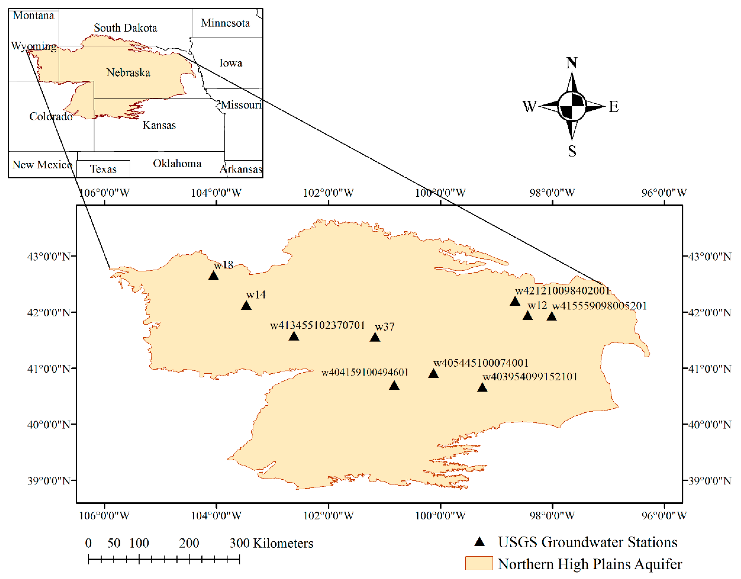
The NHPA underlies around 250,000 km2 from five distinct states: South Dakota, Wyoming, Nebraska, Kansas, and Colorado (Figure 1). Heterogeneous deposition of gravel, sand, clay, and unconsolidated silt make up this unconfined aquifer. Agriculture in the NHPA is highly dependent on groundwater pumping, which plays a vital role in groundwater storage declining, both spatially and temporally. Additionally, periods of rainfall availability are out of phase with periods of water demand, which accelerates declination in the groundwater level [42]. Spatiotemporal variability in the groundwater table needs to be investigated to develop a water distribution policy to meet demand. With an average saturated thickness of approximately 77 m, groundwater tables in the NHPA have varying depths of up to thirty meters below the ground surface.
3. Data Acquisition
3.1. GRACE
In this study, GRACE Release 05 products were collected from three different sources, namely, the Jet Propulsion Laboratory (JPL), the Center for Space Research (CSR), and Geo Forschungs Zentrum Potsdam (GFZ), from 2009 to 2016, with a spatial resolution of 1° × 1° [43]. The effect of redistributing the earth’s lithospheric masses due to the delayed viscoelastic response of ice age deglaciation was adjusted for by applying a glacial isostatic adjustment [44]. The oblateness of the earth’s surface was addressed using a spherical harmonic of degree 2 and order 0 coefficient [45]. A destriping and 300 km wide Gaussian filter were also applied to minimize the effects of correlated errors. The scaling factor of the respective datasets was applied to minimize the uncertainties due to the filtering process. The averaging of all three terrestrial water storage (TWS) datasets was performed before further processing to reduce the bias associated with different process algorithms.
3.2. Global Land Data Assimilation System (GLDAS)
GLDAS is a space- and ground-based integrated observation system which estimates terrestrial water, energy storages, and their transformation more realistically [46]. To capture the physical process, the data from multiple ground- and space-based observations were integrated using sophisticated numerical models. Water and energy cycle processes information was used to fill gaps and minimize errors in the observations. Here, the Noah 2.1 land surface model was used, as it generates data with different spatial resolutions (1° × 1°, 0.25° × 0.25°) with the same temporal scale [47]. In this paper, GLDAS Noah 2.1 was used to obtain BFGR, PCSW, ET, HF, precipitation, RZSM, SM, SSR, SWE, SP, temperature, and WS at both coarse (1° × 1°) and finer (0.25° × 0.25°) spatial scales for each month during the study period. A DEM was downloaded from the National Map Viewer (https://apps.nationalmap.gov/download/) with the resolution of 1/3 arc-second. R scripting was used for spatial resampling (0.25° × 0.25°, 1° × 1°) and calculating other parameters (slope and aspect) from the DEM.
4. Methodology
4.1. Groundwater Storage Changes
The terrestrial water balance approach was used to obtain groundwater storage. From terrestrial water storage change (ΔTWS), anomalies of other vertical water components of the terrestrial water cycle, i.e., soil moisture (ΔSM), snow water equivalent (ΔSWE), and canopy water storage (ΔCWS), computed from GLDAS-Noah 2.1, were removed to calculate the groundwater storage anomaly (ΔGWS), as shown in Equation (1).
ΔGWS = ΔTWS − (ΔSM + ΔSWE + ΔCWS)
The anomaly (Δ) for all components was calculated by maintaining the long term mean from 2009 to 2016.
4.2. In Situ Groundwater Storage
Groundwater monitoring data were obtained from the National Ground-Water Monitoring Network (https://cida.usgs.gov/ngwmn/index.jsp). Ten groundwater monitoring stations were chosen to correspond with GRACE data from 2009 to 2016. Temporal consistency in data was tested while choosing the study period and stations. At first, long-term (2009–2016) average groundwater elevation was subtracted from individual groundwater level measurements to calculate the groundwater level anomaly (GWLA), as shown in Equation (2).
Here, GWL represents the groundwater level and GWLLTM is the long-term (2009–2016) mean for the groundwater head of the same station.
Next, the GWLA was factored by specific yield to obtain the GWSA, as shown in Equation (3). The specific yield of the NHPA was obtained from [48].
In this equation, GWSA represents the GWS anomalies (mm), GWLA = groundwater level anomalies (mm), and Sy = average specific yield.
4.3. RF Model
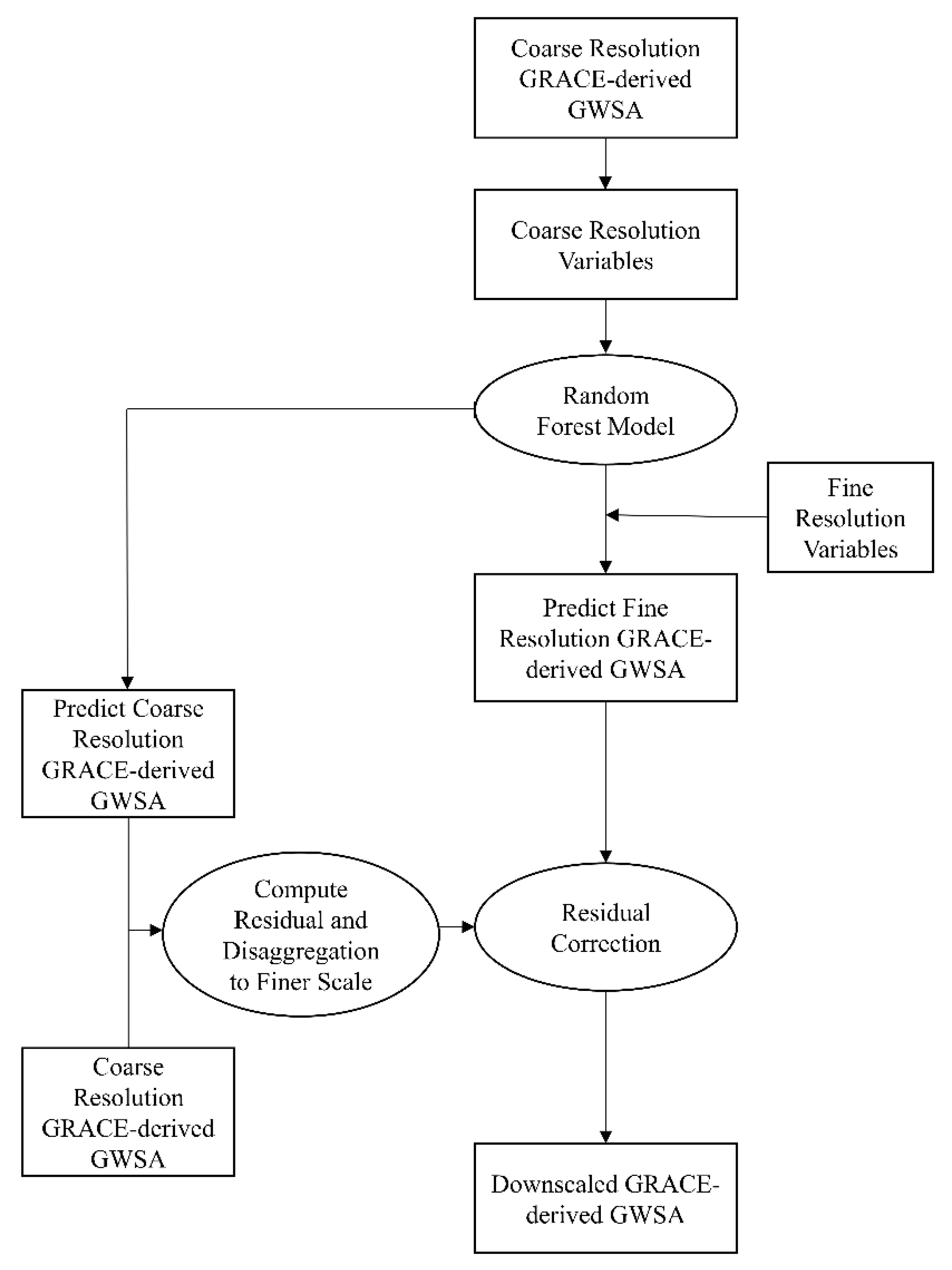
RF is characterized as an ensemble-based nonlinear statistical bagging method. RF generates homogeneous subsets of ancillary predictors, known as regression trees, in a random manner and uses the advantages of using the average results of each combination. At first, it requires several numbers of variables from all predictor variables. The individual regression tree is generated from two-thirds of the bootstrapped sample training data. The remaining one-third of observations are known as out of bag (OOB). Every variable in the RF model generates a non-overlapping predictor space. After selecting the first predictor, the next cut point to split the predictor space was selected by maximizing the reduction in the residual sum of squares error. This process was continued up to a certain stopping criterion. The average value of all the trees, as generated by RF, was considered the model’s prediction. More details on RF can be found in Breiman [29]. OOB error estimates and variable importance rankings are two important features to consider while developing the RF algorithm. A higher number of subsets reduces the confidence of the developed model. On the other hand, using fewer subsets may make it incapable of capturing the appropriate relationship between the variables and the targeted output. It is a common practice to use the square root of the number of predictor variables during classification and one third of the total variables during regression analysis as the number of subsets while developing the RF model. The OOB error is measured by calculating the mean square error difference as a result of using the first two-thirds data and OOB data to generate trees. Once the RF model was trained, it was trained up with multiple of predictor variables and single response variables at the coarse scale. Trained model output was compared with the original response variable to calculate the residual. Then, the model was run using the predictor variable at a finer resolution. The final output, a high-resolution GWSA, was obtained using disaggregated residual correction. A schematic view of applying the RF model is depicted in Figure 2.
5. Results and Discussion
This section first presents the parameter sensitivity of the proposed RF model and then a spatiotemporal evaluation of the proposed RF model.
5.1. RF Result and Parameter Sensitivity
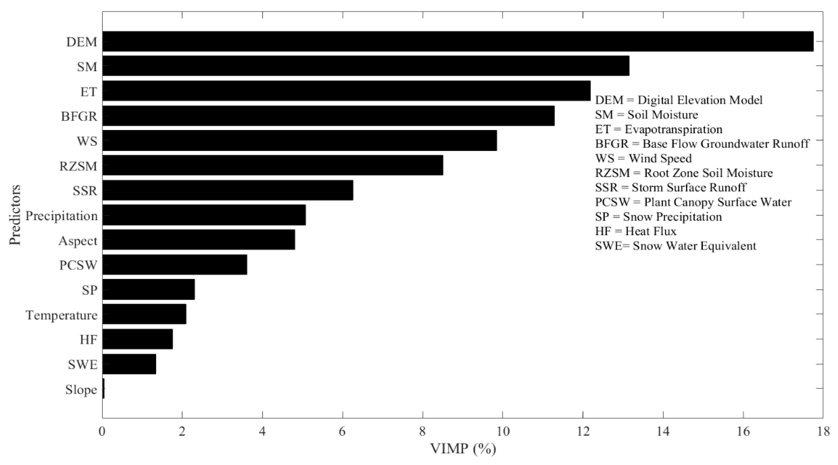
The performance of the RF model mostly depends on selecting appropriate biophysical variables that are highly correlated with GRACE. Precipitation, temperature, DEM, Natural Resources Conservation Service soil data [2,49], evapotranspiration [50], and runoff [51] were used for downscaling GRACE data. In this work, different predictors, i.e., aspect, BFGR, DEM, PCSW, ET, HF, precipitation, RZSM, slope, SM, SSR, SWE, SP, temperature, and WS, were used to develop RF, as those are strongly co-related with groundwater. GRACE data have a lower spatial resolution (1° × 1°). Before applying RF, two hypotheses were considered, i.e., the relation of GRACE to other predictor variables is non-linear, and interactions remain consistent in each spatial direction. To check the applicability of variables, a sensitivity test was performed. The RF can calculate the relative contribution of each variable in the downscaling process. The variable importance measures predictive (VIMP) evaluates the predictive ability of the variables in the developed RF model. VIMP measures the difference in prediction error before and after permutation for each variable. A close-to-zero VIMP indicates the variable has a non-existent or small impact on the prediction. Larger values indicate a higher predictive power. Figure 3 shows the normalized variable importance of the predictors for downscaling within the NHPA. According to Figure 3, out of fifteen variables, DEM was the most crucial predictor with regard to developing RF models. The slope was found to be the least important for predicting the groundwater. The importance calculation adopted was truly statistical and cannot describe any underlying physical processes which increase the importance of the DEM over slope and aspect. Since all the values were greater than zero or positive, all the predictors were considered skillful while estimating the groundwater storage.
Figure 4 shows a schematic diagram of a sample tree which was generated during the training period. This tree can be used for classification using the SM variable at first. For example, if the SM value is less than 235.16 mm the model prediction is done with the left leg and so on. On the other hand, if the SM value is equal, or more than 235.16 mm, it follows that the right offshoot and predictor PCSW has been used. Either SP or PCSW, wherever it reaches, checks the value of the respective predictor from the predictor list and follows the same convention as in the previous step in SM. Every mother node is divided into two child nodes. This step continues until the end node, which gives the value of GWSA. For a set of predictors, different trees of the forest end up with a different output. The result is the simple arithmetic mean of all output resulting from every tree of the forest.
5.2. Evaluation of the RF-Downscaled Data
5.2.1. GWSA Trends in the NHPA
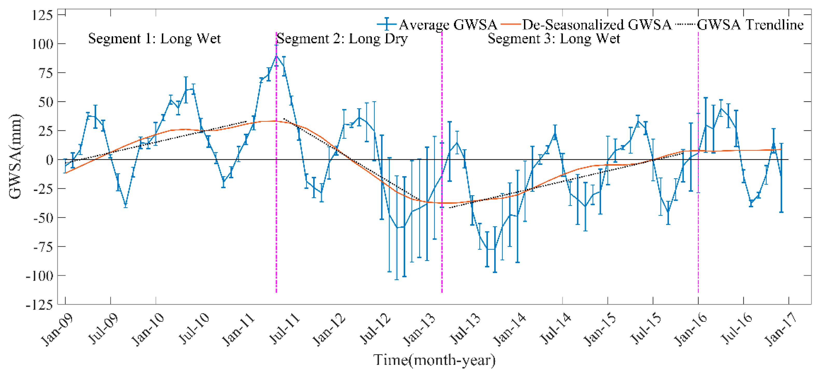
The study time frame was divided according to the appearance of hydrologic extremes, i.e., the big dry, big wet, and fluctuation periods, to evaluate the model’s performance spatially [52]. At first, the trend in the GWSA was extracted using the non-parametric method “seasonal and trend decomposition using Loess,” which is commonly known as STL [53]. The adjacent high and trough of the GWSA trend were used to identify each of the segments of the extreme event. To locate the shift in the trend, a visual inspection was also performed. The monthly average GWSA of all grids in the NHPA from 2009 to 2016 (Figure 5) suggests that the GWSA had apparent seasonal variability, with a maximum and minimum in April and August, respectively. The monthly GWSA long-term trend can be divided into three sections. For instance, it may be described as including a first wet period from January 2009 to May 2011, followed by a dry period from June 2011 to March 2013, and finally a moderately dry scenario from April 2013 to January 2016. The rest of the time displayed a somewhat steady situation and has not been considered here. The first segment represents significant groundwater replenishment of 18 mm/year. Following this, the big dry period can be characterized as having a higher decline (46.68 mm/year). The last period shows a moderate increase in groundwater at a rate of 18.54 mm/year and steady groundwater storage is observed for the rest of the period. All of the trend was calculated with 95% significance. The error bars show the deviations of the GWSA obtained from the three GRACE datasets (CSR, JPL, and GFZ). To find the missing months, the seasonal component adds after imputation the deseasonalized time series [54].
5.2.2. Spatial Distribution of the Downscaled GWSA
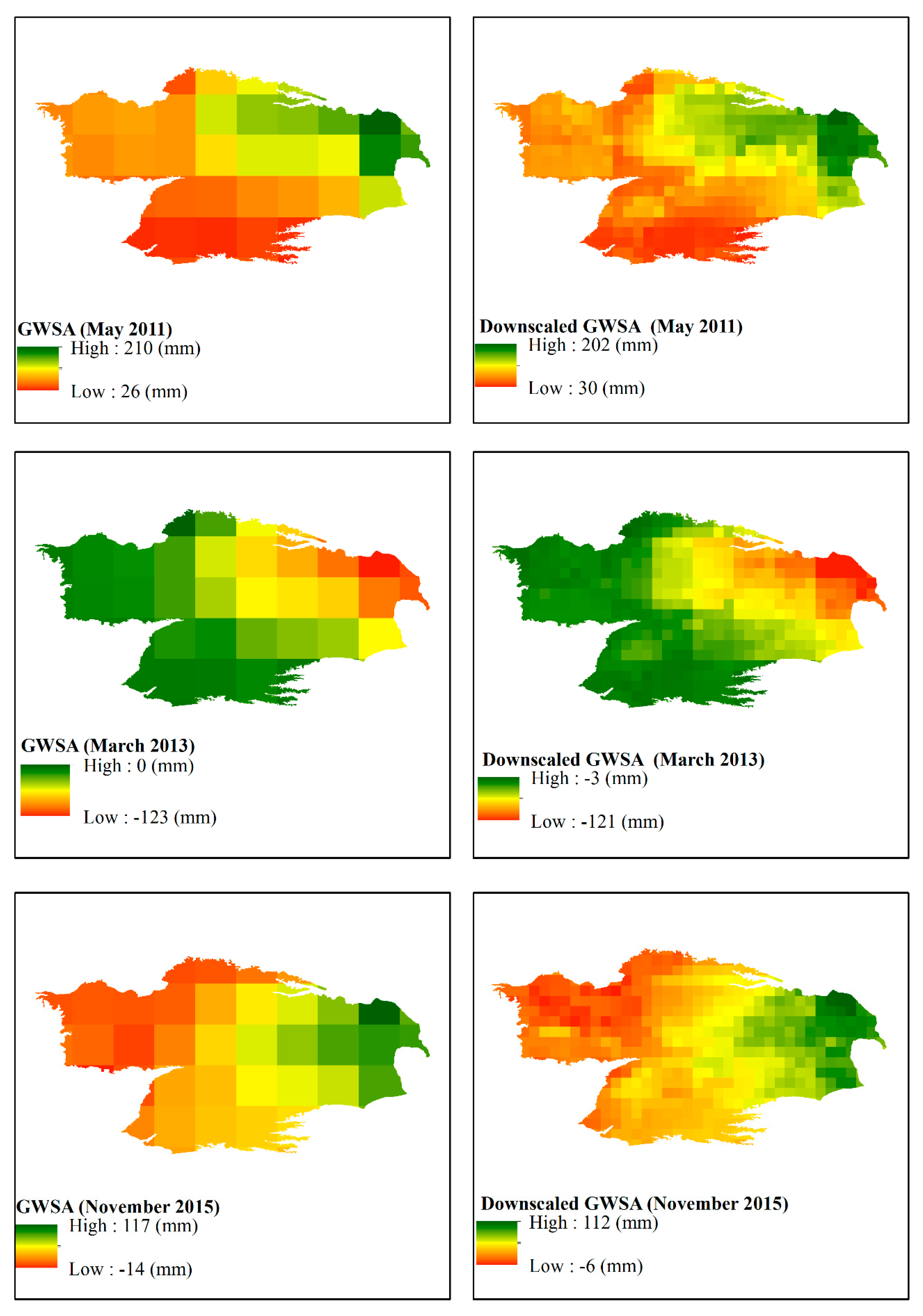
For every hydrologic extreme downscaled GWSA values were plotted. Figure 6 shows the high-resolution GWSA within the NHPA under three different hydrologic extreme conditions. For all three cases, the overall spatial distribution of the high resolution (0.25° × 0.25°) downscaled GWSA was similar to that of the coarse scale (1° × 1°) gridded GWSA. In addition, the downscaled GWSA successfully reflects sub-grid heterogeneity, that is, the effect of local scale geospatial and hydro-climatological characteristics on GWSA. By the end of the first long wet period, the eastern part of the NHPA faced comparatively higher groundwater replenishment. At the end of the long dry period, a completely different scenario was observed; the western part experienced relatively lower depletion than the eastern region. Anomalies indicate that the eastern part of the NHPA experienced a higher variability (−121mm ~ 202mm) in groundwater storage from 2009 to 2016. The central part of the NHPA evidenced steady groundwater table elevations during the study period.
5.2.3. Validation of GWSA with Temporal Scale
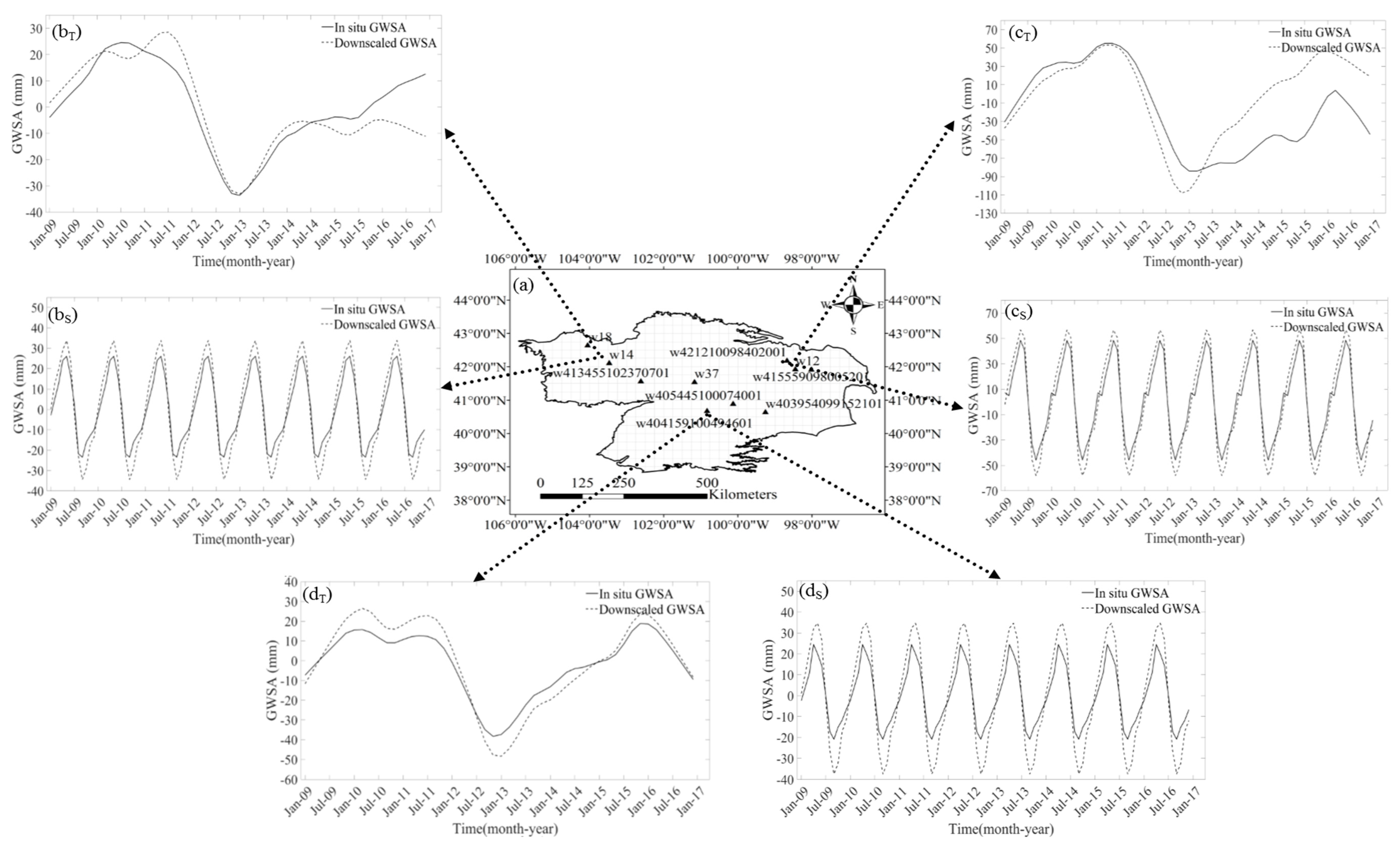
Heterogeneity in aquifer layers results in the nonuniform distribution of the specific yield, thus making groundwater storage calculation more complicated. The temporal patterns of RF-downscaled GWSA were compared with the in situ monitoring station to assess downscaling performance. The long-term temporal variability in GWSA was interpreted by superimposing in situ measurements onto the downscaled product. Figure 7 shows a comparison of in situ water levels and the downscaled GWSA for monthly trends and seasonality for three different observation wells (w14, w12, and w404159100494601) reflecting different regions (east, central, and west) within the NHPA. Both the observed and downscaled GWSA show a fluctuating (moderately increasing, sharply decreasing, steadily increasing) trend from January 2009 to December 2016. Wet conditions up to 2010 support the idea of moderate recharging. The sharp declination in groundwater storage is proof of combined drought and groundwater withdrawals from 2011 to 2013. The steady increasing trend matches recent research in the region which proves that the NHPA experienced groundwater recharging. The seasonal component of monthly GWSA and that observed from in situ stations show strong coherence. Both (downscaled and observed) show the highest value in January and the lowest in July, in a consistent manner.
The statistical indices of all the wells are shown in Table 1. In general, downscaled GWSA showed good conformity with the station values. The Pearson correlation values suggest RF-downscaled GWSA has a statistically significant correlation with the monitoring wells. Out of ten, three wells exhibited very high (0.90 ~ 0.94), and the rest of them high (0.81 to 0.88), positive correlations with the downscaled product. The root mean square error (RMSE) lies between 15.53 mm to 46.69 mm. Table 1 values confirm that it is not always necessarily true that a higher correlation shows a lower RMSE and vice versa. The highest Nash-Sutcliffe efficiency (NSE) among the ten wells is 0.84, for w12. This NSE value indicates that the developed model replicates the observed scenario within a satisfactory range. Percentage bias (PBIAS) suggests the downscaled values slightly overestimate (2.85 ~ 0.09) most of the wells’ measurements, although the highest bias (−14.67, for w37) is estimated as negative. Among the ten wells, the largest PBIAS was evaluated for w37. All these statistical indices indicate that satellite products have the potential to resample GRACE-derived groundwater storage to a finer scale. As the RF-downscaled GWSA replicates the in situ GWSA with a higher correlation, it can be used to enhance the performance of other hydrologic models, i.e., Water – Global Analysis and Prognosis, World Wide Water Resources Assessment, or Land Surface Models (Mosaic, CLSM, or Variable Infiltration Capacity, commonly known as VIC), at the local scale.
6. Uncertainties and Comparison with Previous Studies
The time frame of the current study is short due to consistency in in situ observations; even GRACE does not have long term data with which to take into consideration long-term climate variability. Also, the in situ stations are not dense, which limits the analysis for the validation part. The predictors used for downscaling were not free from error. Additionally, interpolation of missing GRACE may introduce error to the calculation of GWSA. Although the applied method was used to impute time series, a more accurate method like Artificial Neural Network (ANN), associated with other hydrologic variables (for example, rainfall, soil moisture, and precipitation) can be used for future studies. GRACE has latencies from two to six months from the beginning of its launch in April 2002, which might hinder real-time groundwater storage assessment at the local scale.
Recently, Gemitzi and Lakshmi [49] and Miro and Famiglietti [2] have applied ANN to downscale GRACE data. Both models showed good performance with calibration. However, in the validation part, the first one accelerated the overestimation of in situ data. The second one experienced an error of nearly one meter in some places compared to gauge data in the GWSA. Although Seyoum and Milewski [55] have considered the lag effect of predicting variables, the ANN model shows poor performance in terms of its Pearson correlation and exhibits more variability than observed GWSA. On the other hand, the simple statistical approach [50,51] showed comparatively better results. The output of the currently proposed RF model shows an error of less than 8 mm even in extreme hydrologic scenarios. Statistical indices also strengthen the model’s acceptance, as they show high correlation and NSE values compared to the ANN approach. The spatial distribution of GRACE, coupled to an RF, provides an opportunity for assessing groundwater storage more accurately at the regional scale around the world.
7. Conclusions
This study used an RF model, a supervised machine learning approach, to generate a fine resolution GRACE-derived GWSA. The study utilized multiple remote sensing data for a better understanding of groundwater dynamics at regional scales. The downscaling performance of the developed RF model was evaluated by comparing in situ groundwater storage with spatially enhanced GWSA data. The findings of the current research may be summarized as follows.
- (1)
- The RF model was successfully utilized to enhance a GRACE-derived GWSA from coarse (1° × 1°) to finer (0.25° × 0.25°) spatial resolution with acceptable errors.
- (2)
- VIMP shows that the DEM and soil moisture have a comparatively higher impact on the RF-based downscaling process. SWE showed less sensitivity to downscaling, although it is an important component of the terrestrial water cycle.
- (3)
- The RF-based downscaling approach can replicate long-term trends and seasonal variation in groundwater storage variation for individual monitoring wells.
- (4)
- The incorporation of GRACE products with other satellite datasets showed a higher potential to assess groundwater storage variability for comparatively smaller watersheds (less than 772 km2 in equator).
Areas scarce with in situ hydrologic monitoring stations are benefited by spatially-improved GWSA data. The newly developed RF algorithm allows for a better assessment of groundwater storage variability, due to climatic and human activities, on the spatial scale. The integration of more remote sensing data, related to water dynamics, will help to develop a more robust model for setting groundwater management policies in practice at local and regional scales. RF shows its potentiality to overcome the drawbacks of GRACE products. The accuracy of the developed RF model can be justified to the next step when NASA’s newly (May 2018) launched GRACE – Follow On (GRACE-FO) mission data becomes available.
Author Contributions
Conceptualization, M.M.R., A.K., and R.L.; formal analysis, M.M.R.; investigation, M.M.R., B.T., and P.M.; supervision, A.K. and R.L.
Funding
This research received no external funding.
Conflicts of Interest
The authors declare no conflict of interest.
References
- Taylor, C.J.; Alley, W.M. Ground-Water-Level Monitoring and the Importance of Long-Term Water-Level Data; US Geological Survey: Reston, VA, USA, 2002.
- Miro, M.E.; Famiglietti, J.S. Downscaling GRACE Remote Sensing Datasets to High-Resolution Groundwater Storage Change Maps of California’s Central Valley. Remote Sens. 2018, 10, 143. [Google Scholar] [CrossRef]
- Mogheir, Y.; De Lima, J.; Singh, V. Assessment of informativeness of groundwater monitoring in developing regions (Gaza Strip Case Study). Water Resour. Manag. 2005, 19, 737–757. [Google Scholar] [CrossRef]
- Hughes, J.P.; Lettenmaier, D.P. Data requirements for kriging: Estimation and network design. Water Resour. Res. 1981, 17, 1641–1650. [Google Scholar] [CrossRef]
- Kitanidis, P.K.; VoMvoris, E.G. A geostatistical approach to the inverse problem in groundwater modeling (steady state) and one-dimensional simulations. Water Resour. Res. 1983, 19, 677–690. [Google Scholar] [CrossRef]
- Dagan, G. Stochastic modeling of groundwater flow by unconditional and conditional probabilities: 2. The solute transport. Water Resour. Res. 1982, 18, 835–848. [Google Scholar] [CrossRef]
- Hendricks Franssen, H.; Kinzelbach, W. Real-time groundwater flow modeling with the ensemble Kalman filter: Joint estimation of states and parameters and the filter inbreeding problem. Water Resour. Res. 2008, 44. [Google Scholar] [CrossRef]
- Reed, P.; Minsker, B.; Valocchi, A.J. Cost-effective long-term groundwater monitoring design using a genetic algorithm and global mass interpolation. Water Resour. Res. 2000, 36, 3731–3741. [Google Scholar] [CrossRef] [Green Version]
- Strassberg, G.; Scanlon, B.R.; Rodell, M. Comparison of seasonal terrestrial water storage variations from GRACE with groundwater-level measurements from the High Plains Aquifer (USA). Geophys. Res. Lett. 2007, 34. [Google Scholar] [CrossRef] [Green Version]
- Scanlon, B.R.; Longuevergne, L.; Long, D. Ground referencing GRACE satellite estimates of groundwater storage changes in the California Central Valley, USA. Water Resour. Res. 2012, 48. [Google Scholar] [CrossRef] [Green Version]
- Feng, W.; Zhong, M.; Lemoine, J.M.; Biancale, R.; Hsu, H.T.; Xia, J. Evaluation of groundwater depletion in North China using the Gravity Recovery and Climate Experiment (GRACE) data and ground-based measurements. Water Resour. Res. 2013, 49, 2110–2118. [Google Scholar] [CrossRef]
- Vishwakarma, B.D.; Devaraju, B.; Sneeuw, N. What Is the Spatial Resolution of grace Satellite Products for Hydrology? Remote Sens. 2018, 10, 852. [Google Scholar] [CrossRef]
- Zhan, W.; Chen, Y.; Zhou, J.; Wang, J.; Liu, W.; Voogt, J.; Zhu, X.; Quan, J.; Li, J. Disaggregation of remotely sensed land surface temperature: Literature survey, taxonomy, issues, and caveats. Remote Sens. Environ. 2013, 131, 119–139. [Google Scholar] [CrossRef]
- Agam, N.; Kustas, W.P.; Anderson, M.C.; Li, F.; Colaizzi, P.D. Utility of thermal image sharpening for monitoring field-scale evapotranspiration over rainfed and irrigated agricultural regions. Geophys. Res. Lett. 2008, 35. [Google Scholar] [CrossRef] [Green Version]
- Zaitchik, B.F.; Rodell, M.; Reichle, R.H. Assimilation of GRACE terrestrial water storage data into a land surface model: Results for the Mississippi River basin. J. Hydrometeorol. 2008, 9, 535–548. [Google Scholar] [CrossRef]
- Houborg, R.; Rodell, M.; Li, B.; Reichle, R.; Zaitchik, B.F. Drought indicators based on model-assimilated Gravity Recovery and Climate Experiment (GRACE) terrestrial water storage observations. Water Resour. Res. 2012, 48. [Google Scholar] [CrossRef] [Green Version]
- Schumacher, M.; Forootan, E.; van Dijk, A.; Schmied, H.M.; Crosbie, R.; Kusche, J.; Döll, P. Improving drought simulations within the Murray-Darling Basin by combined calibration/assimilation of GRACE data into the WaterGAP Global Hydrology Model. Remote Sens. Environ. 2018, 204, 212–228. [Google Scholar] [CrossRef] [Green Version]
- Forootan, E.; Rietbroek, R.; Kusche, J.; Sharifi, M.; Awange, J.; Schmidt, M.; Omondi, P.; Famiglietti, J. Separation of large scale water storage patterns over Iran using GRACE, altimetry and hydrological data. Remote Sens. Environ. 2014, 140, 580–595. [Google Scholar] [CrossRef]
- Wilby, R.L.; Wigley, T.; Conway, D.; Jones, P.; Hewitson, B.; Main, J.; Wilks, D. Statistical downscaling of general circulation model output: A comparison of methods. Water Resour. Res. 1998, 34, 2995–3008. [Google Scholar] [CrossRef]
- Wilby, R.L.; Charles, S.; Zorita, E.; Timbal, B.; Whetton, P.; Mearns, L. Guidelines for Use of Climate Scenarios Developed from Statistical Downscaling Methods; Supporting material of the Intergovernmental Panel on Climate Change, available from the DDC of IPCC TGCIA; Intergovernmental Panel on Climate Change: Geneva, Switzerland, 2004. [Google Scholar]
- Chiew, F.; Kirono, D.; Kent, D.; Frost, A.; Charles, S.; Timbal, B.; Nguyen, K.; Fu, G. Comparison of runoff modelled using rainfall from different downscaling methods for historical and future climates. J. Hydrol. 2010, 387, 10–23. [Google Scholar] [CrossRef]
- Schoof, J.T. Statistical downscaling in climatology. Geogr. Compass 2013, 7, 249–265. [Google Scholar] [CrossRef]
- Nishii, R.; Kusanobu, S.; Tanaka, S. Enhancement of low spatial resolution image based on high resolution-bands. IEEE Trans. Geosci. Remote Sens. 1996, 34, 1151–1158. [Google Scholar] [CrossRef]
- Mpelasoka, F.; Mullan, A.; Heerdegen, R. New Zealand climate change information derived by multivariate statistical and artificial neural networks approaches. Int. J. Climatol. 2001, 21, 1415–1433. [Google Scholar] [CrossRef]
- Gualtieri, J.; Chettri, S. Support vector machines for classification of hyperspectral data. In Proceedings of the IGARSS 2000, IEEE 2000 International Geoscience and Remote Sensing Symposium, Honolulu, HI, USA, 24–28 July 2000; pp. 813–815. [Google Scholar]
- Yang, M.-D.; Yang, Y.-F. Genetic algorithm for unsupervised classification of remote sensing imagery. In Proceedings of the Image Processing: Algorithms and Systems III, San Jose, CA, USA, 18 January 2004; pp. 395–403. [Google Scholar]
- Fasbender, D.; Tuia, D.; Bogaert, P.; Kanevski, M.F. Support-Based Implementation of Bayesian Data Fusion for Spatial Enhancement: Applications to ASTER Thermal Images. IEEE Geosci. Remote Sens. Lett. 2008, 5, 598–602. [Google Scholar] [CrossRef]
- Hutengs, C.; Vohland, M. Downscaling land surface temperatures at regional scales with random forest regression. Remote Sens. Environ. 2016, 178, 127–141. [Google Scholar] [CrossRef]
- Breiman, L. Random Forests. Mach. Learn. 2001, 45, 5–32. [Google Scholar] [CrossRef] [Green Version]
- Liang, Z.; Tang, T.; Li, B.; Liu, T.; Wang, J.; Hu, Y. Long-term streamflow forecasting using SWAT through the integration of the random forests precipitation generator: Case study of Danjiangkou Reservoir. Hydrol. Res. 2018, 49, 1513–1527. [Google Scholar] [CrossRef]
- He, X.; Chaney, N.W.; Schleiss, M.; Sheffield, J. Spatial downscaling of precipitation using adaptable random forests. Water Resour. Res. 2016, 52, 8217–8237. [Google Scholar] [CrossRef]
- Barrios, J.M.; Ghilain, N.; Arboleda, A.; Gellens-Meulenberghs, F. Evaluating an energy balance setting and random forest-based downscaling for the estimation of daily ET at sub-kilometer spatial resolution. In Proceedings of the 2017 9th International Workshop on the Analysis of Multitemporal Remote Sensing Images (MultiTemp), Brugge, Belgium, 27–29 June 2017; pp. 1–4. [Google Scholar]
- Zhao, W.; Sánchez, N.; Lu, H.; Li, A. A spatial downscaling approach for the SMAP passive surface soil moisture product using random forest regression. J. Hydrol. 2018, 563, 1009–1024. [Google Scholar] [CrossRef]
- Pang, B.; Yue, J.; Zhao, G.; Xu, Z. Statistical Downscaling of Temperature with the Random Forest Model. Adv. Meteorol. 2017, 2017, 7265178. [Google Scholar] [CrossRef]
- Gislason, P.O.; Benediktsson, J.A.; Sveinsson, J.R. Random forests for land cover classification. Pattern Recognit. Lett. 2006, 27, 294–300. [Google Scholar] [CrossRef]
- Daliakopoulos, I.N.; Katsanevakis, S.; Moustakas, A. Spatial downscaling of alien species presences using machine learning. Front. Earth Sci. 2017, 5, 60. [Google Scholar] [CrossRef]
- Nicolas, G.; Robinson, T.P.; Wint, G.W.; Conchedda, G.; Cinardi, G.; Gilbert, M. Using random forest to improve the downscaling of global livestock census data. PLoS ONE 2016, 11, e0150424. [Google Scholar] [CrossRef] [PubMed]
- Folberth, C.; Baklanov, A.; Balkovič, J.; Skalský, R.; Khabarov, N.; Obersteiner, M. Spatio-temporal downscaling of gridded crop model yield estimates based on machine learning. Agric. For. Meteorol. 2019, 264, 1–15. [Google Scholar] [CrossRef]
- Malekipirbazari, M.; Aksakalli, V. Risk assessment in social lending via random forests. Expert Syst. Appl. 2015, 42, 4621–4631. [Google Scholar] [CrossRef]
- Mascaro, J.; Asner, G.P.; Knapp, D.E.; Kennedy-Bowdoin, T.; Martin, R.E.; Anderson, C.; Higgins, M.; Chadwick, K.D. A tale of two “forests”: Random Forest machine learning aids tropical forest carbon mapping. PLoS ONE 2014, 9, e85993. [Google Scholar] [CrossRef] [PubMed]
- Strobl, C.; Zeileis, A. Danger: High Power!–Exploring the Statistical Properties of a Test for Random Forest Variable Importance. In Department of Statistics: Technical Reports, No.17; Ludwig Maximilian University of Munich: München, Germany, 2008. [Google Scholar]
- Jachens, E.; Hutcheson, H.; Thomas, M. Groundwater-Surface Water Exchange and Streamflow Prediction using the National Water Model in the Northern High Plains Aquifer region, USA. In National Water Center Innovators Program Summer Institute Report 2018; Consortium of Universities for the Advancement of Hydrologic Science, Inc.: Cambridge, MA, USA, 2018. [Google Scholar]
- Swenson, S. GRACE Monthly Land Water Mass Grids NETCDF Release 5.0. Ver. 5.0; PO. DAAC: Pasadena, CA, USA, 2012.
- Wahr, J.; Zhong, S. Computations of the viscoelastic response of a 3-D compressible Earth to surface loading: An application to Glacial Isostatic Adjustment in Antarctica and Canada. Geophys. J. Int. 2012, 192, 557–572. [Google Scholar]
- Cheng, M.; Tapley, B.D.; Ries, J.C. Deceleration in the Earth’s oblateness. J. Geophys. Res. Solid Earth 2013, 118, 740–747. [Google Scholar] [CrossRef]
- Rodell, M.; Houser, P.; Jambor, U.; Gottschalck, J.; Mitchell, K.; Meng, C.-J.; Arsenault, K.; Cosgrove, B.; Radakovich, J.; Bosilovich, M. The global land data assimilation system. Bull. Am. Meteorol. Soc. 2004, 85, 381–394. [Google Scholar] [CrossRef]
- Ek, M.; Mitchell, K.; Lin, Y.; Rogers, E.; Grunmann, P.; Koren, V.; Gayno, G.; Tarpley, J. Implementation of Noah land surface model advances in the National Centers for Environmental Prediction operational mesoscale Eta model. J. Geophys. Res. Atmos. 2003, 108. [Google Scholar] [CrossRef]
- Qi, S. Digital Map of Aquifer Boundary for the High Plains Aquifer in Parts of Colorado, Kansas, Nebraska, New Mexico, Oklahoma, South Dakota, Texas, and Wyoming; No. 543; US Geological Survey: Reston, VA, USA, 2010.
- Gemitzi, A.; Lakshmi, V. Downscaling GRACE data to estimate groundwater use at the aquifer scale. In Proceedings of the 15th International Conference on Environmental Science and Technology (CEST), Rhodes, Greece, 31 August–2 September 2017. [Google Scholar]
- Yin, W.; Hu, L.; Zhang, M.; Wang, J.; Han, S.C. Statistical downscaling of GRACE-derived groundwater storage using ET data in the North China Plain. J. Geophys. Res. Atmos. 2018, 123, 5973–5987. [Google Scholar] [CrossRef]
- Ning, S.; Ishidaira, H.; Wang, J. Statistical downscaling of GRACE-derived terrestrial water storage using satellite and GLDAS products. Annu. J. Hydraul. Eng. 2014, 70, I_133–I_138. [Google Scholar] [CrossRef]
- Xie, Z.; Huete, A.; Restrepo-Coupe, N.; Ma, X.; Devadas, R.; Caprarelli, G. Spatial partitioning and temporal evolution of Australia’s total water storage under extreme hydroclimatic impacts. Remote Sens. Environ. 2016, 183, 43–52. [Google Scholar] [CrossRef]
- Cleveland, R.B.; Cleveland, W.S.; McRae, J.E.; Terpenning, I. STL: A Seasonal-Trend Decomposition. J. Off. Stat. 1990, 6, 3–73. [Google Scholar]
- Moritz, S.; Bartz-Beielstein, T. imputeTS: Time series missing value imputation in R. R J. 2017, 9, 207–218. [Google Scholar] [CrossRef]
- Seyoum, W.M.; Milewski, A.M. Improved methods for estimating local terrestrial water dynamics from GRACE in the Northern High Plains. Adv. Water Resour. 2017, 110, 279–290. [Google Scholar] [CrossRef]
Figure 1.
The study area and United States Geological Survey (USGS) well stations.

Figure 2.
Schematic diagram of the groundwater storage anomaly (GWSA) downscaling approach. Legend: GRACE, Gravity Recovery and Climate Experiment.
Figure 2.
Schematic diagram of the groundwater storage anomaly (GWSA) downscaling approach. Legend: GRACE, Gravity Recovery and Climate Experiment.

Figure 3.
Variable important measures predictive (VIMP) (%) of the predictors.

Figure 4.
A sample tree.

Figure 5.
Monthly average GWSA for all the grids of the Northern High Plains aquifer (NHPA).

Figure 6.
GWSA data before and after downscaling at three different hydrologic extremes.

Figure 7.
Trend and seasonal items of measured water levels and GWS anomalies for different stations (a): (b) w14, (c) w12, (d) w404159100494601. Here, T and S indicate the trend and seasonal components of the GWSA, respectively.
Figure 7.
Trend and seasonal items of measured water levels and GWS anomalies for different stations (a): (b) w14, (c) w12, (d) w404159100494601. Here, T and S indicate the trend and seasonal components of the GWSA, respectively.


Table 1.
Statistical indices (Percentage bias (PBIAS), Root Man Square Error (RMSE), Nash-Sutcliffe efficiency (NSE)) comparison between RF-downscaled and in situ GWSA.
Table 1.
Statistical indices (Percentage bias (PBIAS), Root Man Square Error (RMSE), Nash-Sutcliffe efficiency (NSE)) comparison between RF-downscaled and in situ GWSA.
| Gauge Station | Center of Cell | Statistical Indices | ||||
|---|---|---|---|---|---|---|
| Longitude | Latitude | Pearson Correlation | PBIAS | RMSE | NSE | |
| w403954099152101 | −99.875 | 40.875 | 0.81 | −0.88 | 26.90 | 0.62 |
| w18 | −104.125 | 42.625 | 0.88 | 2.85 | 15.71 | 0.74 |
| w14 | −103.375 | 42.125 | 0.86 | 0.34 | 15.53 | 0.74 |
| w421210098402001 | −98.625 | 42.375 | 0.83 | 1.94 | 46.69 | 0.58 |
| w413455102370701 | −102.625 | 41.625 | 0.84 | 0.16 | 16.44 | 0.71 |
| w37 | −101.125 | 41.625 | 0.90 | −14.67 | 23.03 | 0.78 |
| w415559098005201 | −98.125 | 41.875 | 0.88 | 0.09 | 33.18 | 0.75 |
| w12 | −98.375 | 41.875 | 0.92 | 0.46 | 26.48 | 0.84 |
| w404159100494601 | −100.875 | 40.625 | 0.94 | −0.80 | 15.44 | 0.82 |
| w405445100074001 | −102.125 | 40.875 | 0.83 | 0.27 | 16.18 | 0.61 |
© 2019 by the authors. Licensee MDPI, Basel, Switzerland. This article is an open access article distributed under the terms and conditions of the Creative Commons Attribution (CC BY) license (http://creativecommons.org/licenses/by/4.0/).
Share and Cite
MDPI and ACS Style
Rahaman, M.M.; Thakur, B.; Kalra, A.; Li, R.; Maheshwari, P. Estimating High-Resolution Groundwater Storage from GRACE: A Random Forest Approach. Environments 2019, 6, 63. https://0-doi-org.brum.beds.ac.uk/10.3390/environments6060063
AMA Style
Rahaman MM, Thakur B, Kalra A, Li R, Maheshwari P. Estimating High-Resolution Groundwater Storage from GRACE: A Random Forest Approach. Environments. 2019; 6(6):63. https://0-doi-org.brum.beds.ac.uk/10.3390/environments6060063
Chicago/Turabian StyleRahaman, Md Mafuzur, Balbhadra Thakur, Ajay Kalra, Ruopu Li, and Pankaj Maheshwari. 2019. "Estimating High-Resolution Groundwater Storage from GRACE: A Random Forest Approach" Environments 6, no. 6: 63. https://0-doi-org.brum.beds.ac.uk/10.3390/environments6060063
Note that from the first issue of 2016, this journal uses article numbers instead of page numbers. See further details here.