Modeling Height–Diameter Relationships for Mixed-Species Plantations of Fraxinus mandshurica Rupr. and Larix olgensis Henry in Northeastern China


Abstract
:1. Introduction
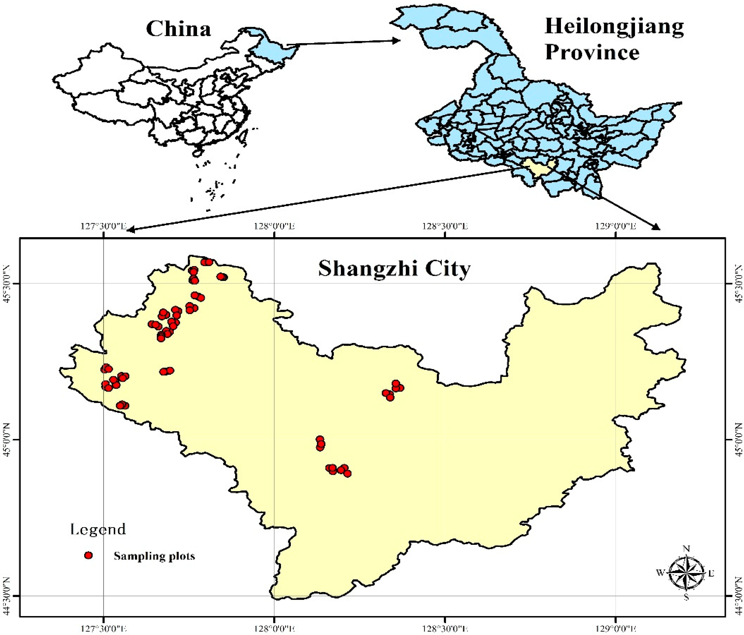
2. Materials and Methods
2.1. Study Sites
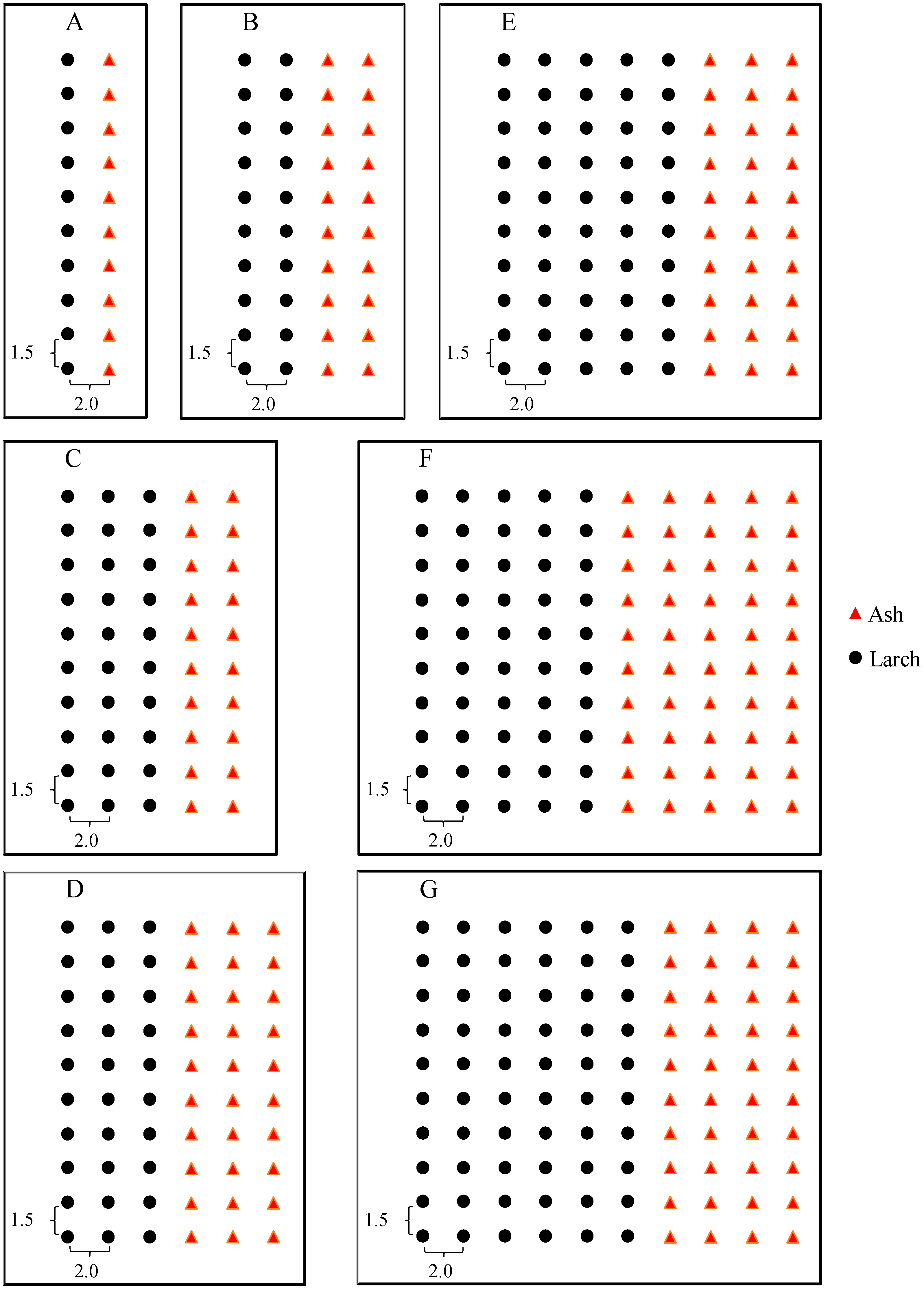
- (A)
- 1-row larch: 1-row ash (1:1)
- (B)
- 2-rows larch: 2-rows ash (2:2)
- (C)
- 3-rows larch: 2-rows ash (3:2)
- (D)
- 3-rows larch: 3-rows ash (3:3)
- (E)
- 5-rows larch: 3-rows ash (5:3)
- (F)
- 5-rows larch: 5-rows ash (5:5)
- (G)
- 6-rows larch: 4-rows ash (6:4)
2.2. Data
2.3. Methods
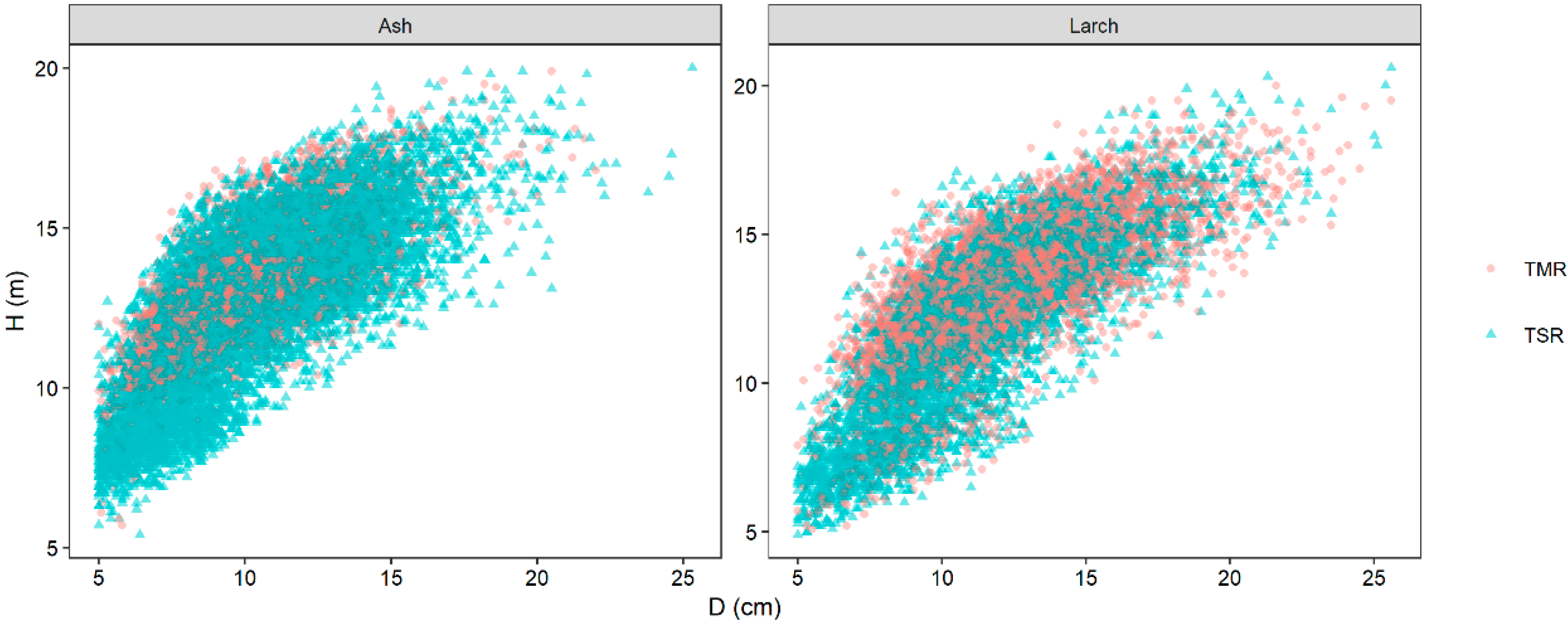
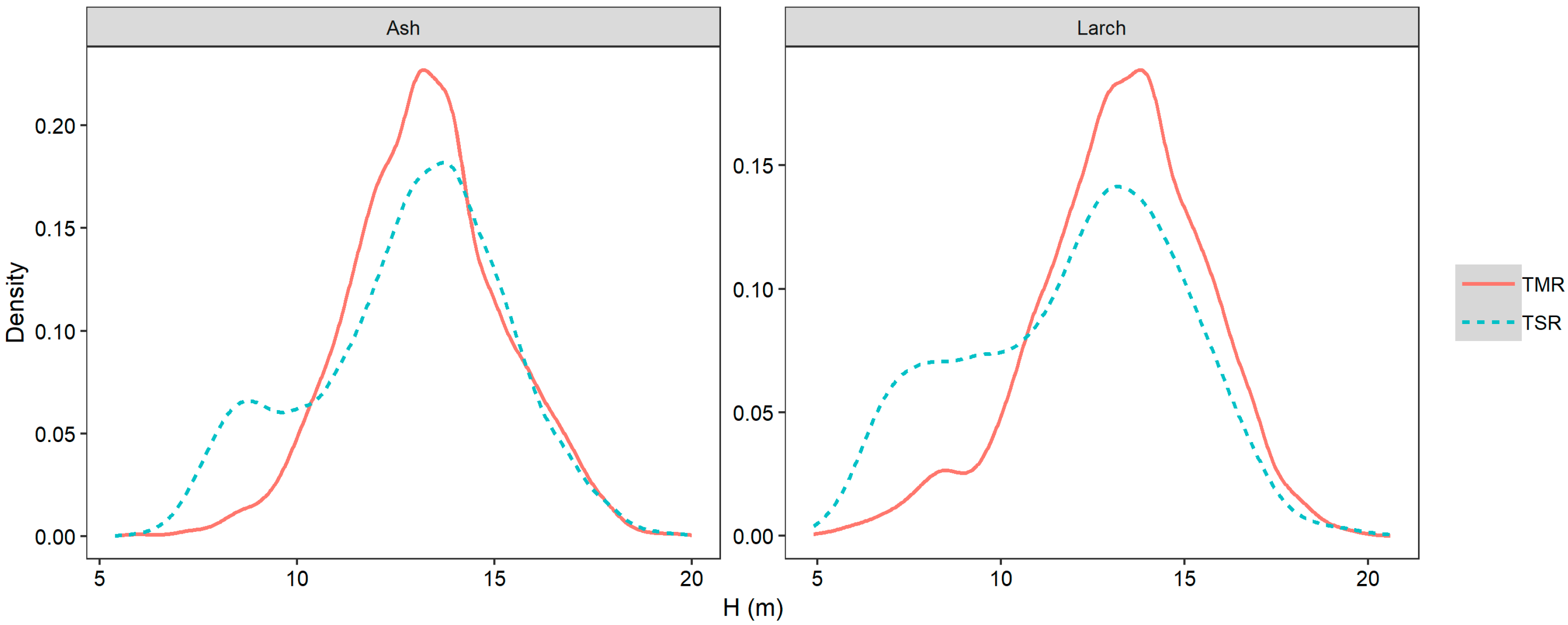
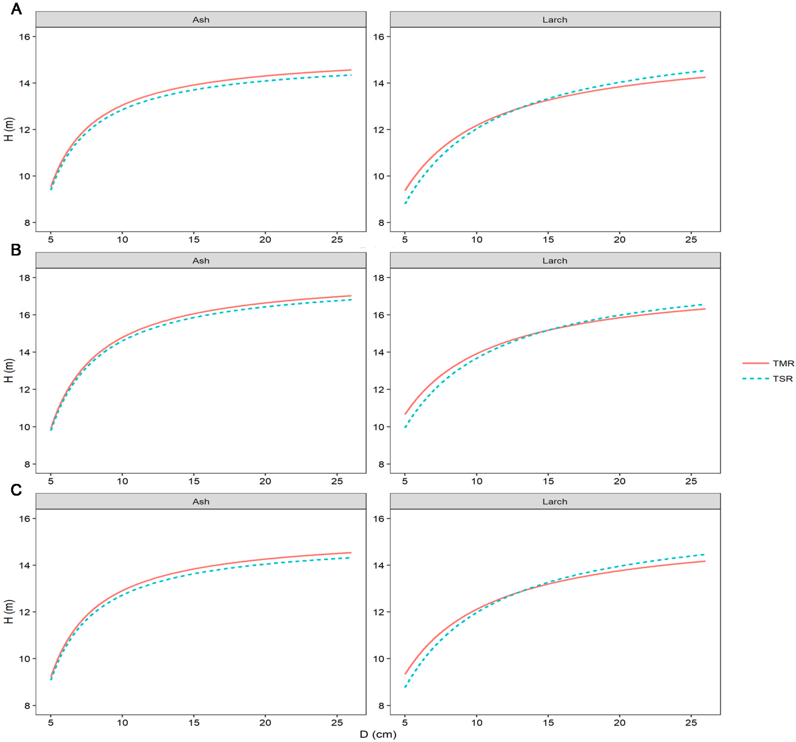
2.3.1. The Comparison of Total Tree Height (H) Between TMR and TSR
2.3.2. Basic Model of H–D Relationship
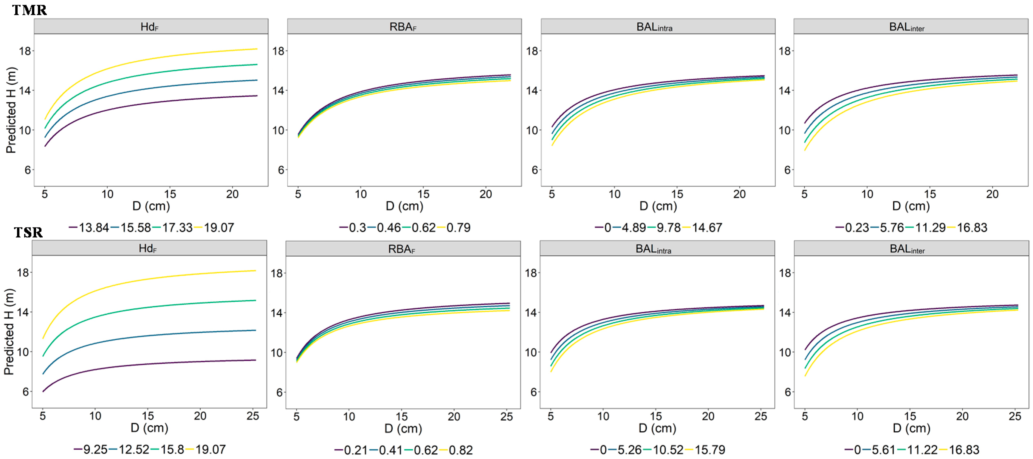
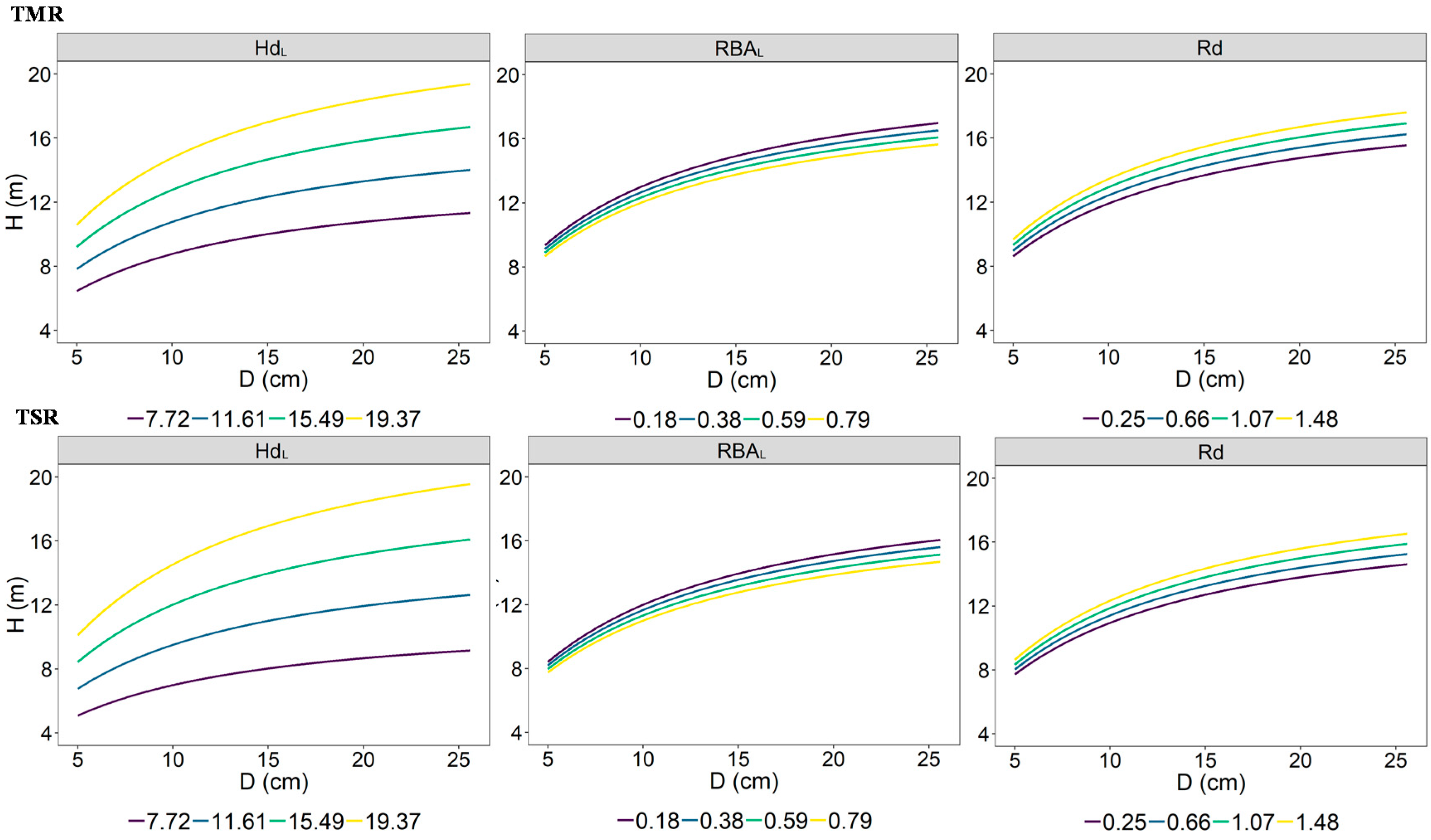
2.3.3. Generalized H–D Model
2.3.4. Mixed-Effects Model
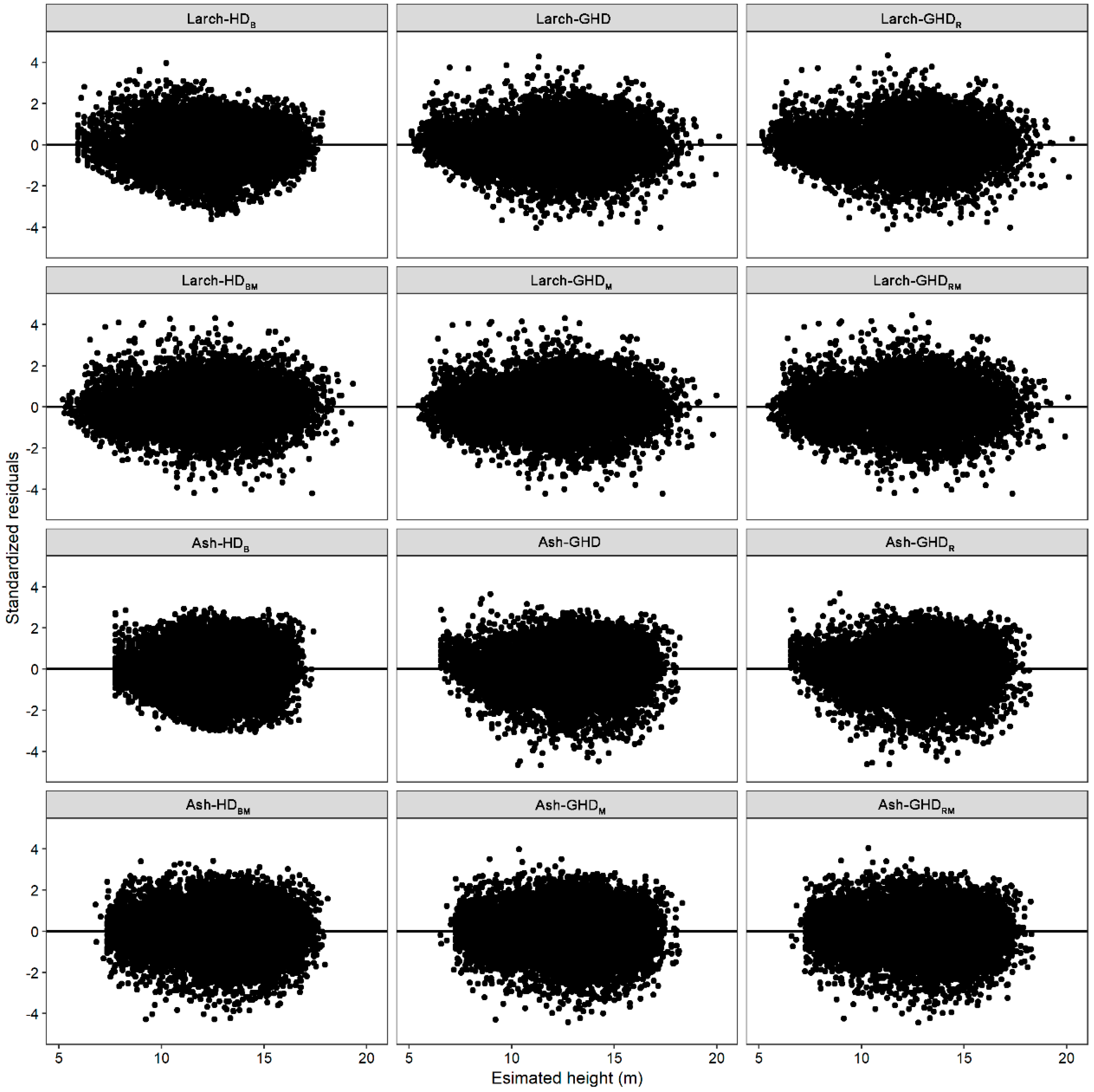
2.3.5. Model Assessment and Validation
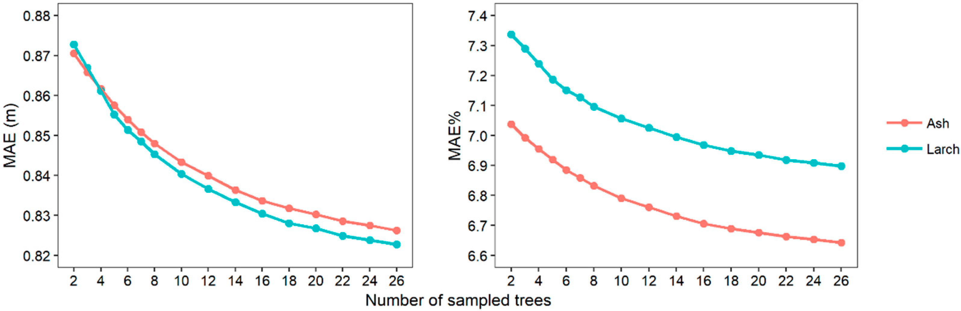
2.3.6. Comparison of Sample Designs
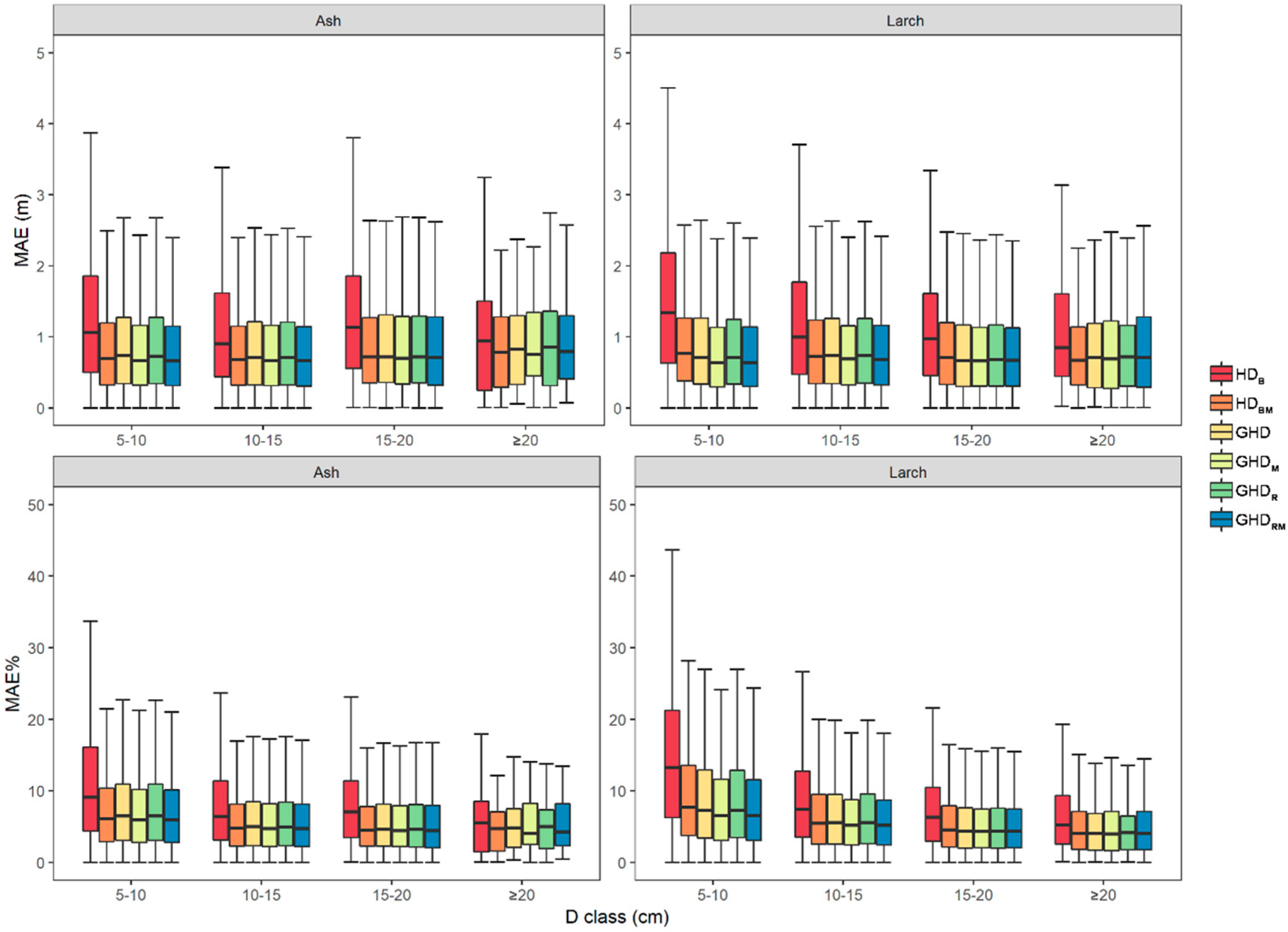
3. Results
3.1. The Variation of H in Different Rows
3.2. Basic H–D Model Results
3.3. Generalized H–D Model
3.4. Mixed-Effects H–D Model
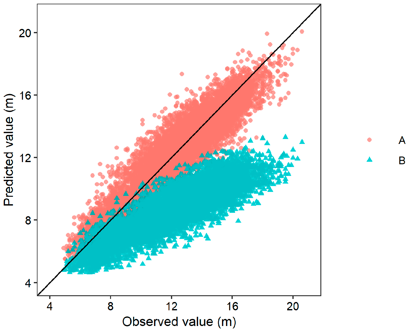
3.5. Model Validation
3.6. Result of the Sampled Designs Comparison
4. Discussion
4.1. Basic H–D Model and Generalized Model
4.2. H–D Model with NLME
4.3. Influence on Species Mixing in H–D Relationship
5. Conclusions
Author Contributions
Funding
Acknowledgments
Conflicts of Interest
References
- Bravo-Oviedo, A. The Role of Mixed Forests in a Changing Social-Ecological World. In Dynamics, Silviculture and Management of Mixed Forests; Springer: Cham, Germany, 2018; pp. 1–25. [Google Scholar]
- Schroeder, P. Carbon storage potential of short rotation tropical tree plantations. For. Ecol. Manag. 1992, 50, 31–41. [Google Scholar] [CrossRef]
- FAO. Global Forest Resources Assessment 2015: How Are the World’s Forests Changing? FAO: Rome, Italy, 2015. [Google Scholar]
- State Forestry and Grassland Administration. The Ninth Forest Resource Survey Report (2014–2018); China Forestry Press: Beijing, China, 2019; p. 451. (In Chinese)
- Bristow, M.; Vanclay, J.K.; Brooks, L.; Hunt, M. Growth and species interactions of Eucalyptus pellita in a mixed and monoculture plantation in the humid tropics of north Queensland. For. Ecol. Manag. 2006, 233, 285–294. [Google Scholar] [CrossRef] [Green Version]
- Ghorbani, M.; Sohrabi, H.; Sadati, S.E.; Babaei, F. Productivity and dynamics of pure and mixed-species plantations of Populous deltoids Bartr. ex Marsh and Alnus subcordata C. A. Mey. For. Ecol. Manag. 2018, 409, 890–898. [Google Scholar] [CrossRef]
- Liu, C.L.C.; Kuchma, O.; Krutovsky, K.V. Mixed-species versus monocultures in plantation forestry: Development, benefits, ecosystem services and perspectives for the future. Glob. Ecol. Conserv. 2018, 15, e00419. [Google Scholar] [CrossRef]
- Manson, D.G.; Schmidt, S.; Bristow, M.; Erskine, P.D.; Vanclay, J.K. Species-site matching in mixed species plantations of native trees in tropical Australia. Agroforest. Syst. 2012, 87, 233–250. [Google Scholar] [CrossRef]
- Prescott, C.E.; Vesterdal, L.; Pratt, J.; Venner, K.H.; Montigny, L.M.D.; Trofymow, J.A. Nutrient concentrations and nitrogen mineralization in forest floors of single species conifer plantations in coastal British Columbia. Can. J. For. Res. 2000, 30, 1341–1352. [Google Scholar] [CrossRef]
- Kanninen, M. Plantation forests: Global perspectives. In Ecosystem Goods and Services from Plantation Forests; Routledge: London, UK, 2010; pp. 1–15. [Google Scholar]
- Moghaddam, E.R. Growth, development and yield in pure and mixed forest stands. Int. J. Adv. Biol. Biom. Res. 2014, 2, 2725–2730. [Google Scholar]
- Piotto, D.; Víquez, E.; Montagnini, F.; Kanninen, M. Pure and mixed forest plantations with native species of the dry tropics of Costa Rica: A comparison of growth and productivity. For. Ecol. Manag. 2004, 190, 359–372. [Google Scholar] [CrossRef]
- Kelty, M.J. The role of species mixtures in plantation forestry. For. Ecol. Manag. 2006, 233, 195–204. [Google Scholar] [CrossRef]
- Piotto, D. A meta-analysis comparing tree growth in monocultures and mixed plantations. For. Ecol. Manag. 2008, 255, 781–786. [Google Scholar] [CrossRef]
- Chaudhary, A.; Burivalova, Z.; Koh, L.; Hellweg, S. Impact of Forest Management on Species Richness: Global Meta-Analysis and Economic Trade-Offs. Sci. Rep. 2016, 6, 23954. [Google Scholar] [CrossRef] [Green Version]
- Pretzsch, H.; Bielak, K.; Block, J.; Bruchwald, A.; Dieler, J.; Ehrhart, H.-P.; Kohnle, U.; Nagel, J.; Spellmann, H.; Zasada, M.; et al. Productivity of mixed versus pure stands of oak (Quercus petraea (Matt.) Liebl. and Quercus robur L.) and European beech (Fagus sylvatica L.) along an ecological gradient. Eur. J. For. Res. 2013, 132, 263–280. [Google Scholar]
- Liziniewicz, M.; Andrzejczyk, T.; Drozdowski, S. The effect of birch removal on growth and quality of pedunculate oak in a 21-year-old mixed stand established by row planting. For. Ecol. Manag. 2016, 364, 165–172. [Google Scholar]
- Wang, X.Y.; Hua, F.Y.; Wang, L.; Wilcove, D.S.; Yu, D.W. The biodiversity benefit of native forests and mixed-species plantations over monoculture plantations. Divers. Distrib. 2019, 25, 1721–1735. [Google Scholar] [CrossRef]
- Forrester, D.I. The spatial and temporal dynamics of species interactions in mixed-species forests: From pattern to process. For. Ecol. Manag. 2014, 312, 282–292. [Google Scholar] [CrossRef]
- Oliveira, N.; Del Río, M.; Forrester, D.I.; Rodríguez-Soalleiro, R.; Pérez-Cruzado, C.; Cañellas, I.; Sixto, H. Mixed short rotation plantations of Populus alba and Robinia pseudoacacia for biomass yield. For. Ecol. Manag. 2018, 410, 48–55. [Google Scholar] [CrossRef]
- Pretzsch, H.; Forrester, D.I.; Rötzer, T. Representation of species mixing in forest growth models. A review and perspective. Eco. Model. 2015, 313, 276–292. [Google Scholar] [CrossRef] [Green Version]
- Pretzsch, H.; Biber, P. Tree species mixing can increase maximum stand density. Can. J. For. Res. 2016, 46, 1179–1193. [Google Scholar] [CrossRef] [Green Version]
- Valsta, L.; Jacobsen, J. Optimizing the Management of European Mixed Forests. In Dynamics, Silviculture and Management of Mixed Forests; Springer: Cham, Germany, 2018; pp. 381–396. [Google Scholar]
- Wang, Q. Spatial distribution of fine roots of larch and ash in the mixed plantation stand. J. For. Res. 2002, 13, 265–268. [Google Scholar]
- Wu, G.; Wang, Z. Individual tree growth-competition model in mixed plantation of manchurian ash and dahurian larch. Chin. J. Appl. Ecol. 2000, 11, 646. (In Chinese) [Google Scholar]
- Wang, Z.; Wu, G.; Wang, J. Application of competition index in assessing intraspecific and interspecif ic spatial relations between manchurian ash and dahurian larch. Chin. J. Appl. Ecol. 2000, 11, 641–645. (In Chinese) [Google Scholar]
- Zou, X.; Yan, Z.; Han, S.; Liu, S.; Huang, G. Effect of mixed planting of Fraxinus mandshurica with Alnus japonica and larix olgensis. Sci. Silvae Sin. 1997, 33, 76–84. (In Chinese) [Google Scholar]
- Zhang, Y. The Relationship between growth and interspecific competition within the ash-larch mixed stand. J. Northeast For. Univ. 1999, 27, 6–9. (In Chinese) [Google Scholar]
- Deng, J.; Zhou, Y.; Yang, L.; Zhang, S.; Li, H.; Wei, Y.; Deng, J.; Qin, S.; Zhu, W. Effects of mixed Fraxinus mandshurica and Larix olgensis plantation on the function diver-sity of soil microbial community. Chin. J. Ecol. 2016, 35, 2684–2691. (In Chinese) [Google Scholar]
- Wang, Q.; Zhang, Y.; Lin, D. Photosynthetic characteristics of ash and larch in mixture and pure stands. J. For. Res. 1997, 8, 144–147. [Google Scholar]
- Mensah, S.; Pienaar, O.L.; Kunneke, A.; Du Toit, B.; Seydack, A.; Uhl, E.; Pretzsch, H.; Seifert, T. Height—Diameter allometry in South Africa’s indigenous high forests: Assessing generic models performance and function forms. For. Ecol. Manag. 2018, 410, 1–11. [Google Scholar] [CrossRef]
- Zang, H.; Lei, X.; Zeng, W. Height–diameter equations for larch plantations in northern and northeastern China: A comparison of the mixed-effects, quantile regression and generalized additive models. Forestry 2016, 89, 434–445. [Google Scholar]
- Özçelik, R.; Hakki, Y.; Yasin, K.; Nevzat, G.; Rüstem, K. Development of Ecoregion-Based Height-Diameter Models for 3 Economically Important Tree Species of Southern Turkey. Turk. J. Agric. For. 2014, 38, 399–412. [Google Scholar] [CrossRef]
- Nogueira, E.M.; Nelson, B.W.; Fearnside, P.M.; França, M.B.; de Oliveira, Á.C.A. Tree height in Brazil’s ‘arc of deforestation’: Shorter trees in south and southwest Amazonia imply lower biomass. For. Ecol. Manag. 2008, 255, 2963–2972. [Google Scholar] [CrossRef]
- Bohora, S.B.; Cao, Q.V. Prediction of tree diameter growth using quantile regression and mixed-effects models. For. Ecol. Manag. 2014, 319, 62–66. [Google Scholar] [CrossRef]
- Gollob, C.; Ritter, T.; Vospernik, S.; Wassermann, C.; Nothdurft, A. A Flexible Height–Diameter Model for Tree Height Imputation on Forest Inventory Sample Plots Using Repeated Measures from the Past. Forests 2018, 9, 368. [Google Scholar]
- Kearsley, E.; Moonen, P.C.J.; Hufkens, K.; Doetterl, S.; Lisingo, J.; Boyemba Bosela, F.; Boeckx, P.; Beeckman, H.; Verbeeck, H. Model performance of tree height-diameter relationships in the central Congo Basin. Ann. For. Sci. 2017, 74, 7. [Google Scholar] [CrossRef] [Green Version]
- Ng’andwe, P.; Chungu, D.; Yambayamba, A.M.; Chilambwe, A. Modeling the height-diameter relationship of planted Pinus kesiya in Zambia. For. Ecol. Manag. 2019, 447, 1–11. [Google Scholar]
- El Mamoun, H.; El Zein, A.I.; El Mugira, M. Height-diameter prediction models for some utilitarian natural tree species. J. For. Prod. Ind. 2013, 2, 31–39. [Google Scholar]
- Sharma, R.P.; Vacek, Z.; Vacek, S.; Kučera, M. Modelling individual tree height–diameter relationships for multi-layered and multi-species forests in central Europe. Trees 2018, 33, 103–119. [Google Scholar] [CrossRef]
- Özçelik, R.; Cao, Q.V.; Trincado, G.; Göçer, N. Predicting tree height from tree diameter and dominant height using mixed-effects and quantile regression models for two species in Turkey. For. Ecol. Manag. 2018, 419–420, 240–248. [Google Scholar]
- Sharma, R.P.; Breidenbach, J. Modeling height-diameter relationships for Norway spruce, Scots pine, and downy birch using Norwegian national forest inventory data. For. Sci. Technol. 2015, 11, 44–53. [Google Scholar] [CrossRef]
- Zheng, J.; Zang, H.; Yin, S.; Sun, N.; Zhu, P.; Han, Y.; Kang, H.; Liu, C. Modeling height-diameter relationship for artificial monoculture Metasequoia glyptostroboides in sub-tropic coastal megacity Shanghai, China. Urban For. Urban Green. 2018, 34, 226–232. [Google Scholar]
- Del Río, M.; Pretzsch, H.; Alberdi, I.; Bielak, K.; Bravo, F.; Brunner, A.; Condés, S.; Ducey, M.J.; Fonseca, T.; Von Lüpke, N.; et al. Characterization of the structure, dynamics, and productivity of mixed-species stands: Review and perspectives. Eur. J. For. Res. 2016, 135, 23–49. [Google Scholar] [CrossRef]
- Alder, D. A distance-independent tree model for exotic conifer plantations in East Africa. For. Sci. 1979, 25, 59–71. [Google Scholar]
- Weibull, W. A statistical distribution function of wide applicability. J. Appl. Mech. 1951, 18, 293–297. [Google Scholar]
- Richards, F. A flexible growth function for empirical use. J. Exp. Bot. 1959, 10, 290–301. [Google Scholar]
- Curtis, R.O. Height-diameter and height-diameter-age equations for second-growth Douglas-fir. For. Sci. 1967, 13, 365–375. [Google Scholar]
- Schreuder, H.T.; Hafley, W.L.; Bennett, F.A. Yield Prediction for Unthinned Natural Slash Pine Stands. For. Sci. 1979, 25, 25–30. [Google Scholar]
- Näslund, M. Skogsförsöksanstaltens Gallringsförsök i Tallskog; Medd. Statens Skogsförsöksanstal: Stockholm, Sweden, 1936. [Google Scholar]
- Bates, D.M.; Watts, D.G. Relative Curvature Measures of Nonlinearity. J. R. Stat. Soc. 1980, 42, 1–25. [Google Scholar] [CrossRef]
- Wykoff, W.R.; Crookston, N.L.; Stage, A.R. User’s Guide to the Stand Prognosis Model; US Department of Agriculture, Forest Service, Intermountain Forest and Range: Washington, DC, USA, 1982. [Google Scholar]
- Schumacher, F.X. New growth curve and its application to timber-yield studies. J. For. 1939, 37, 819–820. [Google Scholar]
- Farr, W.A.; DeMars, D.J.; Dealy, J.E. Height and crown width related to diameter for open-grown western hemlock and Sitka spruce. Can. J. For. Res. 1989, 19, 1203–1207. [Google Scholar]
- Ratkwosky, D.A. Handbook of Nonlinear Regression Models; M. Dekker: New York, NY, USA, 1990. [Google Scholar]
- Huang, S.; Titus, S.J.; Wiens, D.P. Comparison of nonlinear height–diameter functions for major Alberta tree species. Can. J. For. Res. 1992, 22, 1297–1304. [Google Scholar] [CrossRef]
- R Core Team. R: A language and environment for statistical computing. In R Foundation for Statistical Computing; R Core Team: Vienna, Austria, 2019. [Google Scholar]
- Adame, P.; Del Río, M.; Canellas, I. A mixed nonlinear height–diameter model for pyrenean oak (Quercus pyrenaica Willd.). For. Ecol. Manag. 2008, 256, 88–98. [Google Scholar]
- Huang, S.; Price, D.; Titus, S.J. Development of ecoregion-based height–diameter models for white spruce in boreal forests. For. Ecol. Manag. 2000, 129, 125–141. [Google Scholar]
- Widagdo, F.R.A.; Xie, L.; Dong, L.; Li, F. Origin-based biomass allometric equations, biomass partitioning, and carbon concentration variations of planted and natural Larix gmelinii in northeast China. Glob. Ecol. Conserv. 2020, e01111. [Google Scholar] [CrossRef]
- Pinheiro, J.C.; Bates, D.M. Mixed-Effects Models in S and S-Plus; Springer: New York, NY, USA, 2000; p. 528. [Google Scholar]
- Pinheiro, J.; Bates, D.; DebRoy, S.; Sarkar, D. R Core Team, Nlme: Linear and Nonlinear Mixed Effects Models. R package Version 3.1-137. 2018. Available online: https://CRAN.R-project.org/package=nlme (accessed on 20 March 2020).
- Dong, L.; Zhang, L.; Li, F. Additive biomass equations based on different dendrometric variables for two dominant species (Larix gmelini Rupr. and Betula platyphylla Suk.) in natural forests in the eastern Daxing’an Mountains, Northeast China. Forests 2018, 9, 261. [Google Scholar] [CrossRef] [Green Version]
- Crecente-Campo, F.; Corral-Rivas, J.J.; Vargas-Larreta, B.; Wehenkel, C. Can random components explain differences in the height–diameter relationship in mixed uneven-aged stands? Ann. For. Sci. 2013, 71, 51–70. [Google Scholar] [CrossRef] [Green Version]
- Dong, L.; Zhang, L.; Fengri, L.I. A compatible system of biomass equations for three conifer species in Northeast, China. For. Ecol. Manag. 2014, 329, 306–317. [Google Scholar] [CrossRef]
- Wolfe, D.A.; Hollander, M.; Chicken, E. Nonparametric Statistical Methods, 3rd ed.; John Wiley & Sons, Inc.: Hoboken, NJ, USA, 2014; p. 819. [Google Scholar]
- Jong, J.W.F. Rene De Considerations in simultaneous curve fitting for repeated height–diameter measurements. Rev. Can. De Rech. For. 1994, 24, 1408–1414. [Google Scholar]
- Temesgen, H.; Zhang, C.; Zhao, X. Modelling tree height–diameter relationships in multi-species and multi-layered forests: A large observational study from Northeast China. For. Ecol. Manag. 2014, 316, 78–89. [Google Scholar] [CrossRef]
- Coble, A.P.; Cavaleri, M.A. Light drives vertical gradients of leaf morphology in a sugar maple (Acer saccharum) forest. Tree Physiol. 2014, 34, 146–158. [Google Scholar] [CrossRef]
- Riofrío, J.; Del Río, M.; Maguire, D.A.; Bravo, F. Species Mixing Effects on Height–Diameter and Basal Area Increment Models for Scots Pine and Maritime Pine. Forests 2019, 10, 249. [Google Scholar] [CrossRef] [Green Version]


| Variable | Sample Sizes | Mean | Min. | Max. | S.D. | |
|---|---|---|---|---|---|---|
| Stand level | Age (years) | 69 | 18 | 10 | 25 | 4 |
| N (trees·ha−1) | 69 | 1843 | 1060 | 2583 | 374 | |
| NL (trees·ha−1) | 69 | 765 | 240 | 1693 | 318 | |
| NF (trees·ha−1) | 69 | 1079 | 353 | 1717 | 312 | |
| Dq (cm) | 69 | 11.2 | 7.4 | 15.2 | 1.8 | |
| DqL (cm) | 69 | 12.1 | 7.3 | 15.8 | 2.0 | |
| DqF (cm) | 69 | 10.6 | 6.5 | 16.1 | 1.8 | |
| Hd (m) | 69 | 15.5 | 9.7 | 19.4 | 2.4 | |
| HdL (m) | 69 | 14.9 | 7.7 | 19.4 | 2.5 | |
| HdF (m) | 69 | 15.1 | 9.2 | 19.1 | 2.4 | |
| Dd (cm) | 69 | 16.81 | 9.63 | 21.51 | 2.70 | |
| DdL (cm) | 69 | 16.29 | 8.55 | 21.14 | 2.71 | |
| DdF (cm) | 69 | 14.68 | 8.55 | 21.13 | 2.56 | |
| BA (m2·ha−1) | 69 | 17.84 | 7.59 | 24.92 | 3.63 | |
| BAL (m2·ha−1) | 69 | 8.50 | 1.61 | 16.83 | 3.32 | |
| BAF (m2·ha−1) | 69 | 9.34 | 2.98 | 15.80 | 2.82 | |
| RNL | 69 | 0.41 | 0.17 | 0.73 | 0.14 | |
| RNF | 69 | 0.59 | 0.27 | 0.83 | 0.14 | |
| RBAL | 69 | 0.47 | 0.18 | 0.79 | 0.14 | |
| RBAF | 69 | 0.53 | 0.21 | 0.82 | 0.14 | |
| RNLF | 69 | 0.82 | 0.21 | 2.70 | 0.55 | |
| RBALF | 69 | 1.05 | 0.22 | 3.79 | 0.67 | |
| Tree level | Larch in side rows | |||||
| D (cm) | 5190 | 11.4 | 5.0 | 25.6 | 3.4 | |
| H (m) | 5190 | 12.0 | 4.9 | 20.6 | 3.0 | |
| RD | 5190 | 0.69 | 0.25 | 1.48 | 0.17 | |
| RDintra | 5190 | 0.71 | 0.26 | 1.49 | 0.17 | |
| RDinter | 5190 | 0.78 | 0.29 | 1.73 | 0.20 | |
| BAL (m2·ha−1) | 5190 | 9.74 | 0.00 | 24.83 | 5.66 | |
| BALintra (m2·ha−1) | 5190 | 5.69 | 0.00 | 16.82 | 3.38 | |
| BALinter (m2·ha−1) | 5190 | 4.05 | 0.00 | 15.55 | 3.21 | |
| Larch in middle rows | ||||||
| D (cm) | 4479 | 12.3 | 5.0 | 25.6 | 3.3 | |
| H (m) | 4479 | 13.2 | 5.1 | 20.0 | 2.3 | |
| RD | 4479 | 0.68 | 0.26 | 1.55 | 0.17 | |
| RDintra | 4479 | 0.70 | 0.26 | 1.63 | 0.18 | |
| RDinter | 4479 | 0.78 | 0.29 | 1.72 | 0.20 | |
| BAL (m2·ha−1) | 4479 | 10.93 | 0.00 | 24.74 | 6.21 | |
| BALintra (m2·ha−1) | 4479 | 6.71 | 0.00 | 16.80 | 3.79 | |
| BALinter (m2·ha−1) | 4479 | 4.22 | 0.00 | 14.56 | 3.15 | |
| Ash in side rows | ||||||
| D (cm) | 9460 | 10.5 | 5.0 | 25.3 | 3.0 | |
| H (m) | 9460 | 12.8 | 5.4 | 20.0 | 2.5 | |
| RD | 9460 | 0.63 | 0.25 | 1.60 | 0.15 | |
| RDintra | 9460 | 0.72 | 0.25 | 1.90 | 0.17 | |
| RDinter | 9460 | 0.65 | 0.25 | 1.71 | 0.17 | |
| BAL (m2·ha−1) | 9460 | 11.76 | 0.00 | 24.91 | 5.37 | |
| BALintra (m2·ha−1) | 9460 | 5.73 | 0.00 | 15.79 | 3.41 | |
| BALinter (m2·ha −1) | 9460 | 6.03 | 0.00 | 16.83 | 3.29 | |
| Ash in middle rows | ||||||
| D (cm) | 3699 | 10.1 | 5.0 | 22.0 | 2.5 | |
| H (m) | 3699 | 13.3 | 5.7 | 19.9 | 1.9 | |
| RD | 3699 | 0.56 | 0.25 | 1.08 | 0.14 | |
| RDintra | 3699 | 0.66 | 0.28 | 1.25 | 0.15 | |
| RDinter | 3699 | 0.58 | 0.26 | 1.20 | 0.14 | |
| BAL (m2·ha−1) | 3699 | 13.94 | 0.37 | 24.87 | 4.88 | |
| BALintra (m2·ha−1) | 3699 | 6.68 | 0.00 | 14.67 | 2.86 | |
| BALinter (m2·ha−1) | 3699 | 7.26 | 0.23 | 16.83 | 3.18 | |
| Functions Number and Forms | Reference |
|---|---|
| [1] | Curtis, 1967 |
| [2] | Weibull, 1951 |
| [3] | Richards, 1959 |
| [4] | Curtis, 1967 |
| [5] | Schreuder, 1979 |
| [6] | Bates, 1980 |
| [7] | Wykoff, 1982 |
| [8] | Schumacher, 1939 |
| [9] | Farr, 1989 |
| [10] | Ratkowsky, 1990 |
| [11] | Huang, 1992 |
| [12] | Näslund, 1936 |
| Function NO. | Larch | Ash | ||||
|---|---|---|---|---|---|---|
| Ra2 | RMSE | AIC | Ra2 | RMSE | AIC | |
| [1] | 0.6490 | 1.6274 | 36551.17 | 0.5949 | 1.4980 | 48000.48 |
| [2] | 0.6505 | 1.6238 | 36509.48 | 0.5997 | 1.4891 | 47845.45 |
| [3] | 0.6511 | 1.6225 | 36495.03 | 0.6009 | 1.4869 | 47807.14 |
| [4] | 0.6509 | 1.6230 | 36499.19 | 0.5996 | 1.4893 | 47847.50 |
| [5] | 0.6295 | 1.6720 | 37069.57 | 0.5780 | 1.5289 | 48538.71 |
| [6] | 0.6406 | 1.6467 | 36776.98 | 0.5917 | 1.5039 | 48104.73 |
| [7] | 0.6502 | 1.6245 | 36517.13 | 0.5985 | 1.4913 | 47883.26 |
| [8] | 0.6513 | 1.6222 | 36489.04 | 0.6004 | 1.4878 | 47820.95 |
| [9] | 0.6428 | 1.6416 | 36717.57 | 0.5951 | 1.4977 | 47995.33 |
| [10] | 0.6513 | 1.6220 | 36488.64 | 0.6011 | 1.4864 | 47797.80 |
| [11] | 0.6510 | 1.6227 | 36496.60 | 0.6003 | 1.4880 | 47825.59 |
| [12] | 0.6479 | 1.6299 | 36580.49 | 0.5971 | 1.4939 | 47928.45 |
| Terms | HDB | GHD | GHDR | HDBM | GHDM | GHDRM |
|---|---|---|---|---|---|---|
| Fixed Parameters | ||||||
| 19.3542 (0.2054) | 0.9403 (0.2014) | 1.0989 (0.2045) | 15.957 (0.3153) | 0.0192 (0.2353) | 0.0187 (0.2343) | |
| 4.4967 (0.1812) | 0.8947 (0.0081) | 0.2319 (0.0277) | 2.7639 (0.0998) | 0.9842 (0.0105) | 0.2901 (0.0299) | |
| −0.9106 (0.1621) | −0.6741 (0.1585) | 0.8878 (0.0081) | −1.484 (0.1696) | −1.2728 (0.1861) | 0.9773 (0.0103) | |
| 0.7846 (0.0978) | −0.6955 (0.1597) | 0.9683 (0.1858) | −1.2811 (0.185) | |||
| 0.0552 (0.0035) | 0.8572 (0.1025) | 0.0386 (0.0074) | 0.8929 (0.1847) | |||
| 0.0431 (0.0033) | 0.0545 (0.0036) | 0.0437 (0.0114) | 0.0390 (0.0074) | |||
| −2.5907 (0.1104) | 0.0443 (0.0034) | −2.5601 (0.1757) | 0.051 (0.0112) | |||
| −2.4928 (0.1149) | −2.5679 (0.1745) | |||||
| Variance and Covariance | ||||||
| 6.0896 | 0.0022 | 0.0021 | ||||
| −1.8709 | 0.0187 | 0.0170 | ||||
| 0.7876 | 0.6604 | 0.6326 | ||||
| 1.9840 | 0.6526 | 0.6733 | 0.3357 | 0.3180 | 0.3214 | |
| Power of Variance Function | ||||||
| φ | 0.2268 | 0.4106 | 0.3841 | 0.4412 | 0.4620 | 0.4565 |
| Fitting Statistics | ||||||
| Ram2 | 0.5367 | 0.7739 | 0.7755 | |||
| Rac2 | 0.6007 | 0.7799 | 0.7811 | 0.8073 | 0.8073 | 0.8086 |
| RMSE | 1.4866 | 1.1037 | 1.1007 | 1.0327 | 1.0329 | 1.0293 |
| AIC | 47781.92 | 39948.66 | 39878.79 | 38201.22 | 38205.99 | 38115.64 |
| Terms | HDB | GHD | GHDR | HDBM | GHDM | GHDRM |
|---|---|---|---|---|---|---|
| Fixed Parameters | ||||||
| 22.0687 (0.32) | −3.2305 (0.3365) | −2.8436 (0.3659) | 22.1981 (0.3766) | 0.8813 (0.9818) | 1.3128 (1.0437) | |
| 7.3134 (0.2993) | 0.9926 (0.0132) | −0.6354 (0.1554) | 10.7985 (0.6782) | 1.1193 (0.0231) | −0.6404 (0.1943) | |
| −0.3217 (0.2003) | −0.8614 (0.1186) | 1.0035 (0.0146) | 3.7726 (0.4841) | −2.7711 (0.3547) | 1.1434 (0.0254) | |
| 4.5559 (0.2281) | −0.9276 (0.1225) | 2.1637 (0.4704) | −2.8744 (0.3693) | |||
| 2.7125 (0.288) | 4.5772 (0.2324) | 6.1743 (0.7434) | 1.9964 (0.4935) | |||
| −0.7514 (0.3519) | 3.2783 (0.3478) | 1.7318 (0.4936) | 6.7962 (0.8233) | |||
| −0.5494 (0.1211) | −0.5872 (0.1477) | |||||
| Variance and Covariance | ||||||
| 12.5038 | 0.6341 | 0.6223 | ||||
| 6.6646 | ||||||
| 4.9502 | ||||||
| 0.8771 | 0.8660 | 0.8956 | 0.6397 | 0.6729 | 0.6708 | |
| Power of Variance Function | ||||||
| φ | 0.4953 | 0.1894 | 0.1615 | 0.1922 | 0.1740 | 0.1748 |
| Fitting Statistics | ||||||
| Ram2 | 0.5849 | 0.8361 | 0.8365 | |||
| Rac2 | 0.6513 | 0.8399 | 0.8404 | 0.8590 | 0.8568 | 0.8572 |
| RMSE | 1.6220 | 1.0992 | 1.0975 | 1.0314 | 1.0393 | 1.0382 |
| AIC | 36488.65 | 29029.72 | 29002.23 | 27810.19 | 27957.6652 | 27937.7944 |
| Model | Ash | Larch | ||
|---|---|---|---|---|
| MAE (m) | MAE% (%) | MAE (m) | MAE% (%) | |
| HDB | 1.1967 | 9.8683 | 1.3046 | 11.5190 |
| HDBM | 0.8299 | 6.6421 | 0.8789 | 7.6137 |
| GHD | 0.8701 | 7.0340 | 0.8686 | 7.3402 |
| GHDM | 0.8156 | 6.5440 | 0.8117 | 6.7934 |
| GHDR | 0.8682 | 7.0166 | 0.8684 | 7.3366 |
| GHDRM | 0.8095 | 6.4927 | 0.8111 | 6.7883 |
© 2020 by the authors. Licensee MDPI, Basel, Switzerland. This article is an open access article distributed under the terms and conditions of the Creative Commons Attribution (CC BY) license (http://creativecommons.org/licenses/by/4.0/).
Share and Cite
Xie, L.; Widagdo, F.R.A.; Dong, L.; Li, F. Modeling Height–Diameter Relationships for Mixed-Species Plantations of Fraxinus mandshurica Rupr. and Larix olgensis Henry in Northeastern China. Forests 2020, 11, 610. https://0-doi-org.brum.beds.ac.uk/10.3390/f11060610
Xie L, Widagdo FRA, Dong L, Li F. Modeling Height–Diameter Relationships for Mixed-Species Plantations of Fraxinus mandshurica Rupr. and Larix olgensis Henry in Northeastern China. Forests. 2020; 11(6):610. https://0-doi-org.brum.beds.ac.uk/10.3390/f11060610
Chicago/Turabian StyleXie, Longfei, Faris Rafi Almay Widagdo, Lihu Dong, and Fengri Li. 2020. "Modeling Height–Diameter Relationships for Mixed-Species Plantations of Fraxinus mandshurica Rupr. and Larix olgensis Henry in Northeastern China" Forests 11, no. 6: 610. https://0-doi-org.brum.beds.ac.uk/10.3390/f11060610