Article

The Effects of Natural and Economic Factors on the Financial Performance of Forest Management Units: The Example of Forest Districts of the State Forests National Forest Holding from Eastern Poland

1
Department of Forest Resources Management, Faculty of Forestry, University of Agriculture in Krakow, al. 29-listopada 46, 31-425 Krakow, Poland
2
State Forests National Forest Holding, Forest Protection Team in Radom (Workplace in Lublin), ul. Startowa 11, 20-352 Lublin, Poland
*
Author to whom correspondence should be addressed.
Submission received: 1 October 2021 / Revised: 29 October 2021 / Accepted: 8 November 2021 / Published: 11 November 2021
(This article belongs to the Section Forest Economics, Policy, and Social Science)

Abstract

:
Given the changing market conditions and uncertainty arising from climate change, forest management tends to focus on the financial functioning of forest holdings. The objective of this work is to study the financial performance of forest districts using ratio analysis, synthetic financial indicators, as well as the relationship between synthetic indicators and forest district categories defined in terms of forest site type, site fertility, compatibility stand species composition, species composition, harvesting system, harvesting intensity, fragmentation of forest complexes and management difficulty level. The study material consists of financial documentation from 82 forest districts of the State Forests National Forest Holding (SFNFH) in eastern Poland from the years 2015–2019 and 2005–2009 (for comparison purposes). Synthetic indicators were calculated using two sets of financial ratios as well as two variants of accounting data. In the study period, forest districts were found to differ in terms of their financial performance, which was affected by the natural and economic factors. The synthetic indicators were significantly higher (p > 0.05) for forest districts operating on low-fertility lowland sites, those managing stands with dominant pine, and those implementing a clearcutting regeneration system. The findings concerning the effects of selected natural and economic factors on the financial condition of forest districts may be used for financial planning and management by SFNFH, in particular in decision-making processes to optimize forest management. The applied methods may stand as a basis for the construction of a sectoral evaluation tool.

1. Introduction

The increasingly unpredictable crises in the timber market and the growing risks associated with pursuing sustainable forestry practices in the face of climate warming and weather anomalies have forced forest management units (FMUs) to focus on the economic aspects and financial performance of forest holdings [1,2,3,4,5]. Furthermore, under conditions of accelerating economic, social, and political globalization and given the growing demand for timber and other forestry products and services in European countries, FMUs need to optimize their decisions concerning forestry operations and analyze their profitability [6,7,8,9,10]. Forest holdings face numerous challenges in the context of implementing sustainable forest management (SFM) [11], such as nature conservation in forest areas [12], ecosystem services [13,14] a biobased economy [15] and forest certification [16]. The efficiency of forest management is also influenced by climate change and the increasing risk of damage caused by winds, draughts, and insect outbreaks [17,18]. Other significant factors include the organizational system and level of development of forest districts and forest service companies as well as the technologies used by them [19]. These determinants also impact the financial management of forest holdings, which differs considerably from that of other economic entities, such as public sector organizations and state-owned enterprises and private companies. The lack of close correlations between the efforts undertaken and their effects leads to disproportions between expenditures on production and the value of the obtained timber or other forest products [20]. The financial and accounting systems of forest holdings are shaped by the specific natural and economic determinants of forestry production [21,22]. Discrepancies between the production cycle of forest stands and the timing of labor inputs make it difficult to determine the financial outcomes of annual forestry operations [23]. It should also be noted that in addition to harvesting timber State Forests holdings, which pursue SFM, play a major role in delivering crucial public services, such as the conservation of biodiversity as well as water and soil resources [24,25,26]. Non-production forest functions, critical to modern societies and provided free of charge in Poland, entail a financial burden on forest holdings functioning under different natural conditions, which affects their profitability and ability to deliver those functions.
Forest holdings operate under varied natural and economic conditions, which influence the scale of their production, financial outlays, and forest management methods [27,28,29,30]. This means that FMUs operating under favorable conditions gain additional economic benefits in the form of a differential rent, while those operating under less favorable conditions are deprived of such benefits and may struggle to self-finance. Of importance is also the size of forest holdings, as the larger ones enjoy economies of scale due to the lower unit costs of forest management and timber production. It is easier and more profitable for large holdings to integrate forest policy goals with their management objectives as well as conduct forest investment projects, implement technological advances in practice, and take advantage of knowledge and innovation. In turn, the parcelization of forest holdings is problematic in the context of efficient management of forest resources, their productivity, and financial results [31,32].
Numerous authors have researched the economic and financial aspects of forest management, including the optimization of species composition, stand age structure, production cycle, regeneration methods, and timber harvesting and skidding [33,34,35,36,37,38,39]. Callaghan et al. [40] noted that while most management practices have a significant influence on economic efficiency, they differ depending on the region and forest type.
Comprehensive financial analysis involving capital, assets, financial results, and general financial performance is a tool that facilitates rational decision making [10,41,42,43,44,45]. The importance of such analysis increases with the degree of responsibility for the management of enterprises [21]. As a result, from a managerial perspective, it is necessary to seek tools that may be helpful in evaluating and improving efficiency as well as identifying any inefficiencies of forest districts. The analysis of financial indicators (ratio analysis) assesses the performance of economic entities using specific measures of economic activity, but that an accurate interpretation of those indicators is of the essence [46]. The number of financial indicators is practically unlimited, as indicators can be created as needed. The most popular of them are indicators of financial liquidity, profitability, economic activity and debt. Liquidity ratios measure a company’s ability to pay debt obligations. The debt ratio indicates the degree of debt financing. Efficiency ratios measure a company’s ability to use its assets and manage its liabilities effectively in the current period or in the short term. Profitability ratios reveal a company’s ability to earn a satisfactory profit and return on investment. Financial indicators can be compared over time and space, taking into account boundary conditions [47,48]. The need to monitor the finances of FMUs (in Poland SFNFH districts) is associated with the technically and organizationally challenging production conditions, and especially with the fundamental dependence of forest production on the natural environment, long production cycles, and the resulting need for long-term forecasting and planning of forest production [49]. Given the confluence of complicated factors and determinants, analysis of the financial performance of forest districts, as well as cost analysis (which is the subject of a separate publication) are indispensable to maintain and improve the profitability of forestry production in the long-term. Some authors have applied ratio analysis to investigate the economic and financial problems of forest holdings [50,51,52,53].
The literature presents a variety of approaches to the measurement of technical and economic efficiency. The non-parametric approach concentrates on the regularity assumptions of the production possibility set [54]. Data envelopment analysis (DEA) is a methodology extensively applied in measuring the relative efficiency of decision-making units with multiple inputs and outputs [55,56]. The free disposal hull (FDH) is an alternative deterministic, non-parametric model developed for the evaluation of productive efficiency. The DEA-based Malmquist productivity index (MPI) is a good tool for measuring the productivity change of DMUs at different periods of time. In the parametric approach it is assumed that the boundary of the production possibility set can be represented by a functional form with constant parameters [54]. Parametric methods include the stochastic frontier approach (SFA), the distribution free approach (DFA), and the thick frontier approach (TFA). Finally, multiple criteria decision making (MCDM) is an alternative method of evaluation of technical efficiency.
Of interest is the financial performance of SFNFH districts, especially that they operate in varied natural conditions. The financial performance of forest districts and their position in the forestry sector can be evaluated by ratio analysis involving a set of liquidity, efficiency, and profitability indicators. Furthermore, comparative statistical methods may be deployed to construct aggregated indicators with a view to gaining more comprehensive insights. Both are useful in developing management strategies for State Forests units and can be implemented at all management levels in the process of allocating financial surpluses and improving the profitability of forest districts in the long term.
The effects of natural and economic determinants on the financial performance of forest districts are far from clear and have given rise to the following research questions: (1) Are there any statistically significant relationships between synthetic financial indicators and forest district categories defined on the basis of natural factors, such as forest site type (FST), forest site fertility, compatibility between stand species composition and forest site type, and actual tree species composition? (2) Are there any statistically significant relationships between synthetic financial indicators and forest district categories defined on the basis of economic factors (felling system, timber harvesting intensity, fragmentation of forest complexes, management difficulty level)?
The objective of the present work is to analyze the financial performance of forest districts using financial ratios, synthetic indicators, as well as relationships between the synthetic indicators and the natural and economic conditions of forest management. In particular, the study involves:
(1)
Analysis of the financial performance of forest districts based on data from the years 2015–2019 and their comparison with those for 2005–2009;
(2)
Analysis of relationships between synthetic financial indicators and selected natural and economic factors;
(3)
A comparison of synthetic financial indicators based on different methodological models and the verification of their usefulness for assessing the financial performance of forest districts.

2. Materials and Methods

2.1. Characteristics of the Financial Management of the State Forests National Forest Holding and the Subject Matter of the Study

The State Forests National Forest Holding (SFNFH) is a self-financing entity without a legal personality [57,58] which manages 7609 thousand ha of land accounting for 77% of the woodland area of Poland. In contrast to private enterprises, in its operations, SFNFH prioritizes sustainability, environmental protection, and the preservation of forest biodiversity, with economically sound forestry production coming second. SFNFH is supposed to conduct its operations “based on economic considerations”, which means that it needs to continually improve ways of allocating its revenues to accomplish all of its statutory objectives. In the years 1994–2019 timber sales accounted for 78.6–87.2% of SFNFH revenues; in 2019, total SFNFH revenues amounted to PLN (zloty) 9149 million (as compared to total costs of PLN 8710 million).
State Forests units have very limited possibilities of diversifying their revenue sources, which makes their business foundations extremely labile, based on demand for one product only (timber). Despite its significant position in the timber supply market, SFNFH has been implementing changes in the way it manages its resources in order to maintain self-financing operations in the face of continually increasing operating costs. All State Forests units (the General Directorate, 17 regional directorates, and 430 forest districts) follow a uniform accounting policy pursuant to the Chart of Accounts adopted by the State Forests National Forest Holding [59], with the financial year coinciding with the calendar year. SFNFH maintains its accounts and prepares its financial statements pursuant to the Polish Accounting Act [60]. A unique feature of SFNFH is its Forest Fund, which is designed to compensate forest districts for any financial shortfalls arising from their forest management operations. Forest Fund resources, which are distributed at the central level by the SFNFH Director-General, may be also allocated to other goals, such as investments and the stabilization fund. Forest districts make contributions to the Forest Fund on a monthly basis depending on their revenues from timber sale; those contributions add to their costs and subtract from their profits and financial results. On the other hand, if the contribution is lower than the amount of Forest Fund subsidy they receive, the difference (the so-called basic subsidy) will reduce their costs, increasing their revenues and financial results [61,62,63].
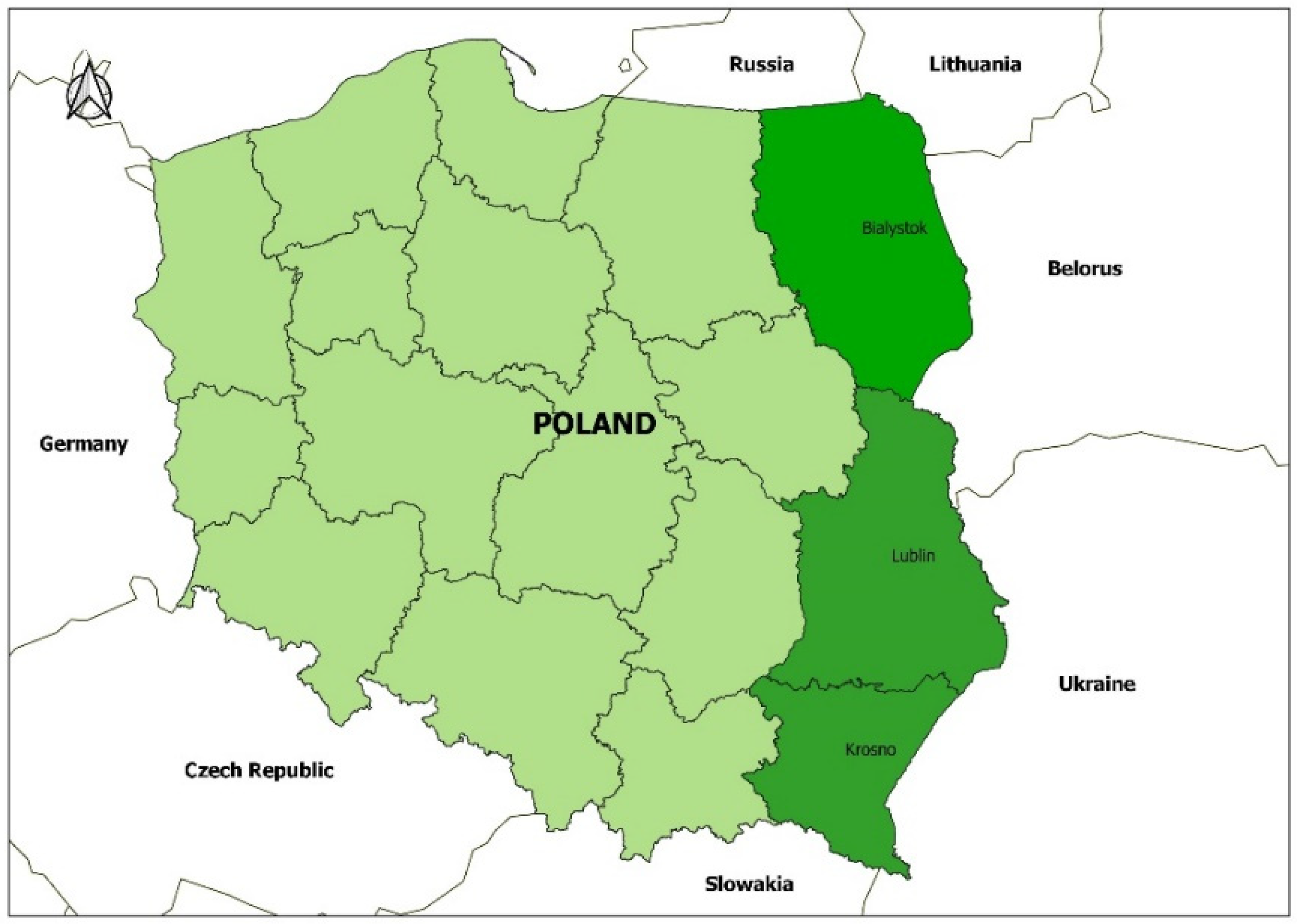
The present study encompassed 82 forest districts (the basic organizational units of SFNFH) belonging to the Białystok, Krosno, and Lublin State Forests Regional Directorates (SFRDs) in south-eastern, eastern, and north-eastern Poland (Figure 1). These forest districts are located in areas characterized by comparable levels of economic development and a similar business environment. They also engage in similar marketing activities due to the specific structure of the wood processing industry; while facilities processing medium-diameter timber are highly concentrated, few pulp or paper mills are located in proximity of the above SFRDs; on the other hand, facilities processing large-diameter timber are scattered but they are found in the vicinity of large forest complexes in each of these SFRDs.
SFRD Białystok administers an area of 625,222 ha with a forest cover of 29.6%; SFRD Krosno administers 418,250 ha with a forest cover of 36.3%, and SFRD Lublin administers 420,400 ha with a forest cover of 22.2%. The studied area is quite varied in terms of forest site types (FSTs): montane FSTs occupy 160.9 thousand ha (11.9% of the total), upland FSTs cover 122.0 thousand ha (9.1%), while lowland FSTs occupy 1064.1 thousand ha, accounting for the largest share of the study area (79.0%). These proportions roughly reflect the distribution of FSTs on the scale of the whole country. In terms of the main forest tree species, the greatest area is occupied by Scots pine (695.3 thousand ha, or 52.0% of the overall study area), followed by oaks (110.1 thousand ha, or 8.2%), European beech (103.9 thousand ha, or 7.8%), birch (7.6%), Norway spruce (88.2 thousand ha, or 6.6%), and silver fir (78.7 thousand ha, or 5.9%). The average age of the studied stands (60 years) was higher than the average age of all stands managed by SFNFH (62 years in SFRD Białystok, 73 years in SFRD Krosno, and 65 years in Lublin SFRD).
In 2015 SFRD Białystok harvested 2987.9 thousand m3 of timber at a mean price of 182.31 PLN/m3, SFRD Krosno harvested 1886.2 thousand m3 at 184.65 PLN/m3, and SFRD Lublin harvested 2056.2 thousand m3 at 189.50 PLN/m3. The corresponding data for 2019 are 2952.5 thousand m3 at 191.20 PLN/m3 for SFRD Białystok, 2029.7 thousand m3 at 199.74 PLN/m3 for SFRD Krosno, and 2139.6 thousand m3 at 199.39 PLN/m3 for SFRD Lublin [64,65].

2.2. Data

The source of data for the present study was financial documentation from 82 SFNFH forest districts. The following information from the State Forest Information System (SILP) was made available by SFNFH bureaus as well as SFRD Białystok, SFRD Krosno, and SFRD Lublin for the years 2005–2009 and 2015–2019: (1) revenues, costs, and financial results excluding Forest Fund transfers; (2) basic financial statement items, such as State Forests equity, fixed and working assets, and liabilities; (3) annual reports on forest district activity (LPIR-1); (4) economic analyses concerning the performance of SFRDs, and (5) timber sales reports (“Acer”—LPIO-9). The financial statements of individual forest districts (balance sheets, profit and loss accounts, and cash flows) for the years 2005–2009 and 2015–2019 were also used.
Data on the environmental conditions of forestry operations were obtained from forest management plans for the studied forest districts, SFRD reports, as well as forest area and stock updates from the State Forests. Information about land areas was taken from the land register of the State Forests (LPIR-4). Data on management difficulty in forest districts were obtained from the BLP-344 report “Management difficulty indices for the organizational units of the State Forests: Methodology adjustment and updated results” commissioned by the State Forests [29,66,67].

2.3. Classification Criteria and Categories of Forest Districts

In order to determine the effects of selected natural and economic factors on the financial performance of the analyzed entities, forest districts were grouped into categories that are homogeneous (to the extent possible) in terms of those factors. Forest district categories were defined by cluster analysis using the k-means method [68] according to the following criteria: (1) natural criteria—forest site type (FST), site fertility, the degree of compatibility between stand species composition and site type, stand species composition and (2) economic criteria—stand regeneration method (felling system), harvesting volume, the degree of fragmentation of forest complexes and management difficulty level.
In the classification of forest districts by forest site type, the main site groups (coniferous, broad-leaved, upland, and montane) were defined on the basis of water abundance, fertility, and elevation. Those with an overall share exceeding 1.0% of the study area were used for the classification of forest districts in terms of the percentage share of site types; these were: fresh coniferous forest (FCF), fresh mixed coniferous forest (FMCF), moist mixed coniferous forest (MMCF), fresh mixed broadleaved forest (FMBF), moist mixed broadleaved forest (MMBF), boggy mixed broadleaved forest (BMBF), fresh broadleaved forest (FBF), moist broadleaved forest (MBF), alder swamp forest (ASF), alder-ash swamp forest (AASF), fresh upland broadleaved forest (FUBF), fresh montane broadleaved forest (FMontBF).
The classification of forest districts by site fertility was based on a modified site fertility index, Wz [69]:
W z = i = 1 n p i w i i = 1 n p i
where:
  • p i —area of the i-th group of forest sites;
  • w i —degree of fertility of the i-th group of forest sites;
Forest sites were assigned to fertility categories as follows;
I: DCF (dry coniferous forest), SCF (swamp coniferous forest), SHMontCF (swamp high-mountain coniferous forest), SMontCF (swamp montane coniferous forest);
II: FCF (fresh coniferous forest), MCF (moist coniferous forest), SMCF (swamp mixed coniferous forest), FHMontCF (fresh high-mountain coniferous forest, MHMontCF (moist high mountain coniferous forest), FMontCF (fresh montane coniferous forest), MMontCF (moist montane coniferous forest);
III: FMCF (fresh mixed coniferous forest), MMCF (moist mixed coniferous forest), SMBF (swamp mixed broadleaved forest), FUCF (fresh upland mixed coniferous forest), MUMCF (moist upland mixed coniferous forest), MontMCF (montane mixed coniferous forest), FMontMCF (fresh montane mixed coniferous forest);
IV: FMBF (fresh mixed broadleaved forest), MMBF (moist mixed broadleaved forest), AF (alder forest), FUMBF (fresh upland mixed broadleaved forest), MUMBF (moist upland mixed broadleaved forest), FMontMBF (fresh montane mixed broadleaved forest), MMontMBF (moist montane mixed broadleaved forest);
V: FBF (fresh broadleaved forest), MBF (moist broadleaved forest), RF (riparian forest), AAF (alder-ash forest), FUBF (fresh upland broadleaved forest), MUBF (moist upland broadleaved forest, URF (upland riparian forest), UAAF (upland alder-ash forest), FMontBF (fresh montane broadleaved forest), MMontBF (moist montane broadleaved forest), MontRF (montane riparian forest), MontAAF (montane alder-ash forest).
The classification of forest districts by stand species composition was done by comparing the relative volumes of the main forest tree species: Scots pine, Norway spruce, silver fir, European beech, and oaks.
In terms of compatibility between the species composition of stands and the forest site types they occupy (stand-site compatibility), forest districts were divided into three categories based on the relative areas of compatible, partially compatible, and incompatible stands. The percentage share of stands with different degrees of stand-site compatibility was calculated based on information obtained from forest management plans for the studied forest districts according to Formula (2):
U = p P × 100
where:
  • U—the percentage share of stands with a given degree of stand-site compatibility;
  • p—area of stands with a given degree of stand-site compatibility;
  • P—total area of stands in the forest district;
Forest districts were also classified in terms of management difficulty levels according to the methodological assumptions and indicators adopted by the State Forests for evaluating the performance of forest districts [28,29].
As far as the degree of fragmentation of forest complexes is concerned, forest districts were classified based on the concentration indicator (Wk) defined as a quotient of the spatial range of a given forest district [ha] and the area actually managed by it [ha].
Forest districts were also classified into homogeneous groups based on felling systems: clearcutting (designated as I) and mixed systems (designated as II, III, IV, V), taking into account the volume of timber harvested in the years 2005–2009 and 2015–2019.
Finally, forest districts were grouped in terms of the intensity of harvesting operations expressed as the volume of timber harvested per unit of woodland area (m3/ha).

2.4. Ratio Analysis as a Tool for Evaluating the Financial Performance of Forest Districts

Financial indicators include liquidity, activity (efficiency), debt (solvency), and profitability ratios. Liquidity ratios reflect the ability of an enterprise to meet its current obligations. Activity ratios show how quickly an enterprise pays its debts and collects receivables as well as how effectively it manages its inventory. Profitability indicators express the relationship between operating profits, net sales revenues, total assets, and equity [47,70,71]. The profitability of forest districts is primarily determined by their costs (optimized by the State Forests management) and revenues, which depend on natural conditions (volume and quality of timber) and market demand. An enterprise’s debt position is described by the debt ratio and the debt to equity ratio. The optimal value of the debt ratio is thought to be between 57% and 67% [46,72].
The financial performance of forest districts was evaluated by calculating financial ratios excluding Forest Fund effects on financial records. Aggregated (synthetic) indicators were computed using two sets of financial ratios: (1) the Universal Model (adopted by State Forests units) and (2) the model proposed by Buraczewski and Wysocki [73] (Table 1). Calculations were done in two accounting variants: including and excluding Forest Fund transfers from the balance sheets and profit and loss accounts.
The Universal Model assesses the financial performance of forest districts by means of liquidity, profitability, activity, and debt ratios. Buraczewski and Wysocki’s model [73] places a greater emphasis on an enterprise’s debt position, paying less attention to activity ratios. Based on substantive considerations and statistical analysis of the variability and correlations between the ratios, two sets of liquidity, debt, activity, and profitability ratios were used for the calculation of synthetic indicators (Table 1).

2.5. Evaluation of the Financial Performance of Forest Districts Using Synthetic Financial Indicators

Using a synthetic indicator, a forest district can be characterized by means of a single figure adopting values from the range [0, 1] (the closer it is to unity, the better the financial performance of the forest district). Three synthetic indicators were analyzed:
(1)
Synthetic indicator 1—built according to the State Forests’ Universal Model, excluding Forest Fund transfers from financial records;
(2)
Synthetic indicator 2—built according to the Universal Model, including Forest Fund transfers in financial records;
(3)
Synthetic indicator 3—built according to the model proposed by A. Buraczewski and F. Wysocki [73], excluding Forest Fund transfers from financial records.
The synthetic financial indicators were constructed using an unsupervised method due to the considerable diversity of the analyzed organizational units. The point of departure for building synthetic indicators was a data matrix [X] containing diagnostic variables, i.e., economic indicators characterizing the studied forest districts (3).
X = [ X 11 X 1 K X n 1 X N K ]
where
  • matrix rows (n = 1 … N) represent forest districts;
  • matrix columns (k = 1 … K) represent financial indicators calculated for the forest districts.
Analytical matrices for the periods 2015–2019 and 2005–2009 were constructed based on two sets of financial indicators: nine ratios from the Universal Model used in practice by forest districts, or alternatively eight ratios from the model proposed by Buraczewski and Wysocki [73]. Prior to defining synthetic indicators, the diagnostic variables (stimulants, destimulants, and nominants) were normalized [74]. Stimulants are indicators with high desirable values, destimulants are those with low desirable values, while nominants are variables for which optimal values can be determined.
Subsequently, the mean normalized values of the diagnostic variables describing the financial performance of forest districts were calculated from Formula (4):
Z i = K 1 k = 1 K Z i k , ( i = 1 ,   ,   N )
where
  • zi—value of the synthetic indicator,
  • zik—value of the normalized variable.

2.6. Data Analysis Methods

Financial indicators were calculated using the same methodological assumptions for both study periods. Statistical analysis was used to evaluate the significance of differences between the independent variables (natural and economic conditions of forest district operations) and the dependent ones (synthetic indicators). Prior to this analysis, the variables were tested for normality of distribution using the Kolmogorov–Smirnov, Lilliefors, and Shapiro–Wilk tests. Since their distributions were non-normal, a non-parametric rank test was applied. Quantitative variables for three and more groups were compared using the Kruskal–Wallis test. Upon detecting significant differences, the post hoc Dunn test was performed to identify significantly different groups. The statistical significance level was adopted at p < 0.05.
Quantitative variables for three and more measurements were compared by means of the Friedman test. Upon detecting statistically significant differences, post hoc analysis was done by means of the Wilcoxon paired test with Bonferroni. Analysis was implemented in R version 4.1.0 [75].

3. Results

3.1. Forest District Classification according to Natural and Economic Criteria

Five categories of forest districts were distinguished based on forest site types. The first category revealed a dominance of lowland coniferous forest sites (FCF—33.19% and FMCF—26.68%), the second one was characterized by lowland sites (FMCF—34.96% and FMBF—23.17%), the third one predominantly featured lowland broadleaved sites, the fourth one mostly consisted of upland sites (FUBF—72.72%), and the fifth one predominantly contained fresh montane broadleaved forest sites (FMontBF—88.87%) (Table A1).
The site fertility index was used to classify forest districts into very high, high, low, and very low fertility categories. In the first category, the site fertility index ranged from 2.171 to 2.946 with a mean of 2.635, while in the fourth category it was from 4.523 to 4.974 (Table A2).
Three categories were distinguished in terms of compatibility between stand species composition and forest site type. The mean stand-site compatibility index was 0.58 for forest districts placed in the “compatible” category, 1.23 for those in the “partially compatible” category, and 1.62 for those in the “incompatible” category (Table A3). Four forest district categories were found for stand species composition; the first one was characterized by a dominance of pine trees (on average 85.5%), while the fourth one predominantly contained beech (41.9%) and fir trees (35.2%) (Table A4).
Additionally, three categories were defined for the dominant stand regeneration system (timber felling system), with the first category corresponding to a prevalence of clearcutting and the third one representing mixed systems. Furthermore, forest districts were divided into three homogeneous categories depending on harvest volume per 1 ha of woodland (Table A5 and Table A6).
Another indicator reflected the proportion of land managed by a forest district to the spatial range of that district. Again, three distinct groups of forest districts were found with the mean values of this indicator being 2.55, 6.18, and 11.95. Finally, four categories of forest districts were distinguished with respect to the degree of management difficulty. The mean value of this indicator was 16.593 for the first category as compared to 28.704 for the fourth one (Table A7 and Table A8).

3.2. The Financial Performance of Forest Districts as Measured by Indicators

The mean values (as well as medians and quartiles) of the liquidity ratios in the years 2015–2019 were lower as compared to 2005–2009. The activity ratios were more favorable in the years 2015–2019, in which the average payment and inventory turnover periods (DSI) were shorter (25 and 13 days, respectively). In turn, the mean ACP was shorter in 2005–2009 (approx. 13 days). The medians of profitability ratios: ROS, ROA, and ROE assumed negative values (from −0.06 to −3.61) in 2015–2019, while they were slightly above zero (0.06–0.88) in 2005–2009 (Table 2).

3.3. Relationships between Natural Factors and the Synthetic Indicators

3.3.1. Forest Site Types

The present analyses revealed some statistically significant relationships between the synthetic indicators and the natural and economic conditions of forestry operations. The Kruskal–Wallis test showed significant differences between forest district categories distinguished with respect to forest site type and the synthetic indicators (p < 0.05). Additionally, the Dunn test showed differences between various groups of forest districts. Synthetic indicator 1 was significantly higher for forest districts in the lowland mixed forest site category (C) as compared to the lowland broadleaved (A), upland (D), and montane categories (E); it was also significantly higher in the lowland broadleaved (A) and lowland coniferous (B) forest site categories as compared to the montane districts. In turn synthetic indicator 2 was significantly lower in the montane category and synthetic indicator 3 was significantly higher in the lowland mixed category than in the remaining ones. In the years 2005–2009, synthetic indicators 1 and 3 were significantly lower in the montane category (E) than in all other categories, while synthetic indicator 2 was significantly lower in the montane category as compared to the lowland mixed and lowland coniferous forest site categories (Table 3).
The highest median and mean values of synthetic indicator 1, amounting to 0.42, were found for lowland mixed forest site districts; this indicator also exhibited the highest mean and median values in 2005–2009 for the same forest site types (in the latter period these metrics were identical to those calculated for lowland coniferous and upland sites). Indicator 1 exhibited the highest variability for lowland broadleaved sites (0.005–0.54). Higher median, mean, and maximum values were found for indicator 2. The greatest variability was revealed by indicator 3 for lowland broadleaved forest site types (Figure 2).

3.3.2. Forest Site Fertility

In order the answer the question of exactly which categories of forest districts differ, Dunn tests were performed. In the years 2015–2019, synthetic indicators 1 and 2 (p < 0.05) were significantly higher in the group of forest districts managing very low fertility sites as compared to the other categories. In addition, the indicators were significantly higher in forest districts managing low fertility sites as compared to those managing very fertile sites. Synthetic indicator 3 was significantly greater for the very low fertility category than for the low fertility one; moreover the values of synthetic indicator 3 for both of these categories were significantly higher than those for the very high and high fertility groups. In the years 2005–2009 synthetic indicator 3 was significantly lower for the very high fertility category as compared to the other analyzed categories (Table 4).
The synthetic indicators revealed the greatest variability in the case of fertile and very fertile sites. Synthetic indicator 1 was much lower for forest districts managing very fertile sites. Quartile analysis showed that in 2015–2019 the indicator was 0.4 (Q1-first quartile) or less for 75% of forest districts managing very low fertility sites and 0.48 (Q3) or more for 25% of such districts. In turn, in 2005–2009 the corresponding values for low and very low fertility sites were from 0.24 (Q1) to 0.29 (Q3). Both the mean and median values of the indicators reached the highest values for very low and low fertility sites, with little variability (Figure 3).

3.3.3. Compatibility between Stand Species Composition and Forest Site Type

No statistically significant correlations were found between the synthetic indicators and forest district categories distinguished on the basis of compatibility between stand species composition and forest site type (p > 0.05) for either of the two analyzed periods.

3.3.4. Tree Species Composition

The Kruskal–Wallis test showed significant differences between forest district catego-ries, and Dunn test identified differences between individual groups of forest districts. In terms of the species composition of stands, in 2015–2019 synthetic indicators 1 and 3 were significantly higher in the group of forest districts classified in the pine category as compared to the pine + spruce and fir + beech categories. Synthetic indicator 2, excluding Forest Fund transfers, was significantly higher in the pine and pine + oak categories as compared to the fir + beech category. In the years 2005–2009, synthetic indicators 1 and 3 were significantly higher in the pine category than in the pine + oak and fir + beech categories. In the same period of time synthetic indicator 2 was significantly higher for forest districts with dominant pine as compared to the other categories (Table 5).
As regards forest districts where pine was the dominant species, quartile analysis shows that synthetic indicator 1 for the years 2015–2019 amounted to 0.34 or less in 75% of the cases and 0.45 or more in 25% of the cases (Figure 4).

3.4. Relationships between Economic Factors and the Synthetic Indicators

3.4.1. Felling System

All three indicators for the years 2015–2019 as well as synthetic indicator 2 for 2005–2009 were significantly higher in the clearcutting category as compared to the remaining categories. In turn, in 2005–2009 synthetic indicator 3 was significantly higher for clearcutting than for selective cutting (Table 6).
The means and medians of the synthetic indicators were higher in forest districts in the clearcutting category, while the highest indicator variability was found for forest districts with a dominance of mixed and selective cutting systems (Figure 5).

3.4.2. Timber Harvest Intensity

In the years 2015–2019 there were no statistically significant relationships between the synthetic indicators and the volume of harvested timber (p > 0.05). In turn, in 2005–2009 all three indicators were significantly higher for forest districts exhibiting very high harvesting intensity as compared to the other two categories (Table 7).

3.4.3. Fragmentation of Forest Complexes

In the years 2015–2019, synthetic indicator 2 was significantly lower for the low fragmentation group of forest districts as compared to the remaining groups. No statistically significant differences were found for synthetic indicators 1 and 3 in either of the analyzed periods (Table 8).

3.4.4. Management Difficulty Level

In the years 2015–2019 synthetic indicator 2 was significantly higher for the “difficult” category as compared to the “very difficult” one (Table 9). No significant relationships were identified in the 2005–2009 period.

3.5. The Financial Performance of Forest Districts Evaluated by the Synthetic Indicators

The Friedman test showed that the three presented synthetic indicators differed significantly in the analyzed periods (p < 0.05). Wilcoxon paired tests with Bonferroni correction revealed that indicators 2 and 3 were significantly higher than indicator 1 (Table 10).

4. Discussion

This study applied the ratio analysis to evaluate the financial condition of forest districts and the impact of natural and economic factors on the economic situation of forest districts. Ratio analysis is designed to reveal certain salient relationships between financial records. It helps to identify strengths and weaknesses in the business activity of an enterprise, pointing to threats as well as areas of opportunity [72,73,76]. The performed financial analysis provided knowledge about the level and differentiation of the values of financial ratios. In the study, financial ratios calculated for forest districts in the years 2015–2019 exhibited greater stability as compared to 2005–2009 due to the favorable economic conditions prevalent during the former period.
The studied forest districts were characterized by overliquidity, with all liquidity ratios exceeding their reference values (1.6, 1.2, and 0.2) [42]. This was not caused by excessive timber inventories or a long receivable turnover ratio, but rather by the accumulation of excessive financial assets, which generated “opportunity costs” with respect to the market interest rates. Capital management strategy involving high levels of current assets and low levels of current liabilities led to overliquidity affecting from the profitability of forest districts. The efficiency ratios of forest districts for recent years showed an improvement on 2005–2009 in terms of days sales of inventory (13 days). While low DSI values are beneficial in that they signify low levels of stocks which are quickly replenished, care should be taken by forest districts to ensure sufficient inventory levels for meeting their contractual obligations and satisfying the demand for their products within a reasonable period of time. Indeed, the goal of inventory management is to maintain stocks at levels enabling smooth operations at the lowest possible costs [72,76]. Moreover, the differences observed in efficiency ratios indicate a preference for the payment of liabilities. The debt ratio for the years 2015–2019 amounted to 26.92%; it was higher than that for 2005–2009 (14.01%), but it still fell short of the recommended 57–67% range (at the same time, it points to the high financial independence of forest districts). The profitability of the analyzed forest districts was low due to their capital management strategies. Return on sales was lower in the period 2015–2019 (less than −0.52% in 75% of forest districts, and more than 6.0% in 25%). This was in part attributable to the insufficient marketing efforts of forest districts, which were not able to identify additional sources of demand and counter declining timber prices.
Given the low ROE of forest districts, they should intensify investment activity to improve the utilization of their equity and prevent the process of decapitalization occurring in some of them. The lowest financial indicators and the worst financial performance was found for forest districts managing stands belonging to the Białowieża Promotional Forest Complex due to the prioritization of conservation efforts over timber production in that area.
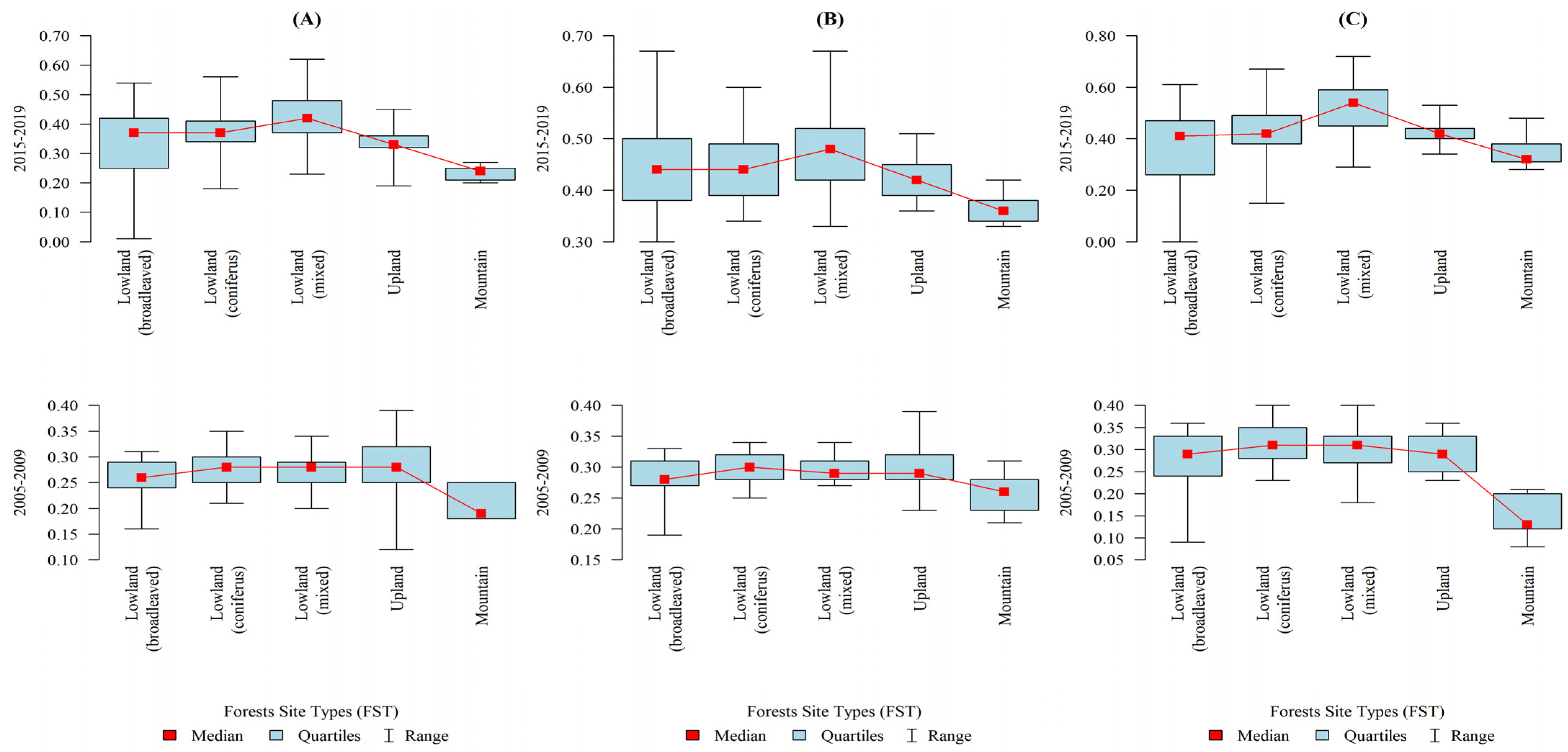
The present analyses partially corroborated the hypotheses concerning differences between the synthetic financial indicators and selected natural and economic conditions of forest district operations. However, the statistical significance differences was between the various categories of forest districts distinguished on the basis of natural and economic factors depending on the applied synthetic indicator (its underlying methodology). It was shown that the financial performance of forest districts depends on FHT. Significant differences were found between forest district categories distinguished on the bases of that factor. In 2015–2019 synthetic indicator 1, which excluded the effects of Forest Fund transfers, was significantly higher for forest districts managing lowland sites as compared to those managing upland and montane sites. The best financial results were obtained in lowland habitats, while forest districts operating in mountain conditions were characterized by the lowest economic efficiency. Similar results were obtained for the years 2005–2009, when montane forest districts exhibited significantly lower values of synthetic indicator 1 as compared to the lowland and upland ones. Additionally, Młynarski et al. [10], who used data envelopment analysis (DEA), found that lowland forest districts exhibited high financial efficiency levels.
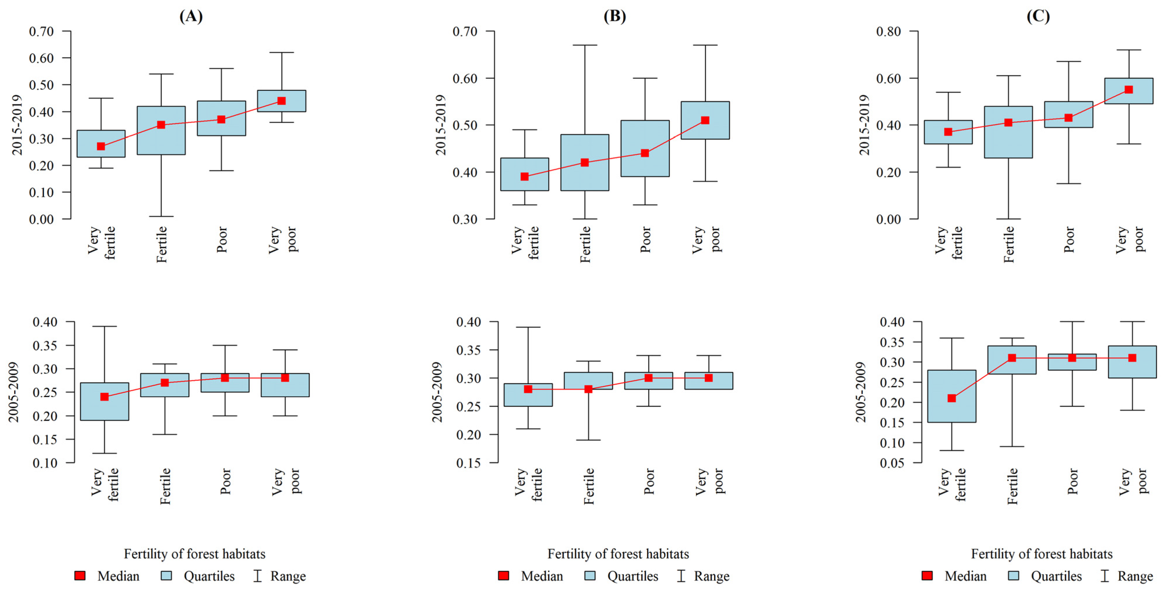
In terms of site fertility, the synthetic indicator was significantly higher for the very nutrient-poor sites typical of coniferous forests, especially when compared to the very fertile sites typical of broadleaved forests. It was thought that forest districts managing the more fertile high productivity sites would exhibit higher values of the synthetic indicator because silver fir stands of 1st quality class should yield 965 m3 of timber per ha at 100 years as compared to 584 m3/ha for pine stands of the same quality and age [77]. The present results were probably affected by market factors related to timber sales, the quality of the assortments produced, as well as operational costs. Lysik [45] reported that unit costs of forestry activities are higher in lowland forest districts managing the more fertile sites (vs. the less fertile ones). The highest unit costs were incurred by montane forest districts, where it is difficult to use economically efficient methods of timber harvesting and skidding.
No statistically significant differences in financial performance as determined by the synthetic indicators were found between the forest district categories distinguished on the basis of compatibility between stand species composition and forest site types.
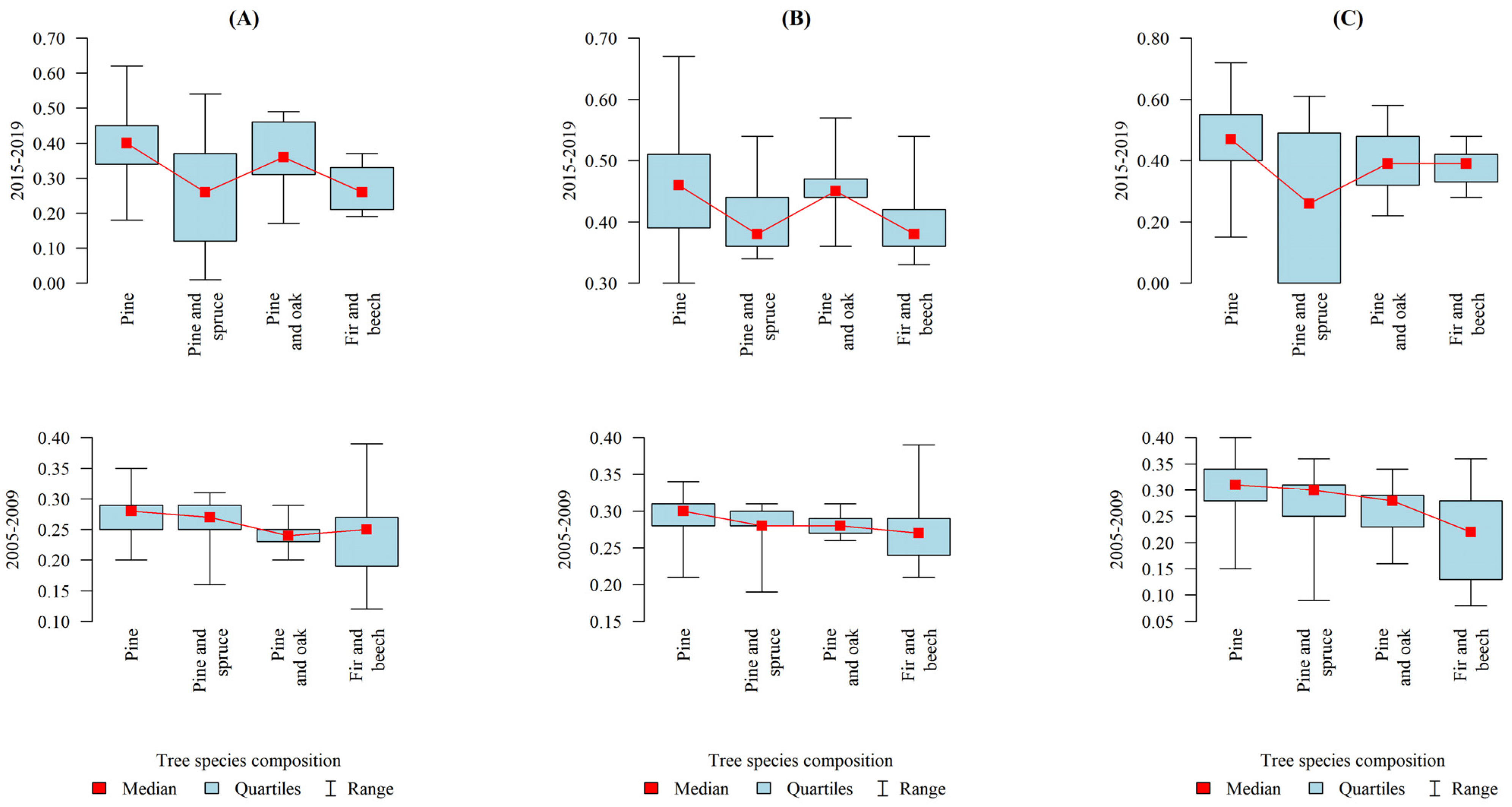
Our research has shown that there are significant relationships between the species composition of stands and the financial condition of forest districts. The establishment of stands by forest holdings is a matter of investment and financial considerations, with the strategic investment goals being reflected in the selection of tree species [78]. Mixed and uneven-aged stands are preferable for environmental reasons and with a view to reducing silvicultural hazards, also in the context of climate change (increasingly severe droughts and winds) [3,79,80,81,82,83]. In terms of species composition, synthetic indicators 1 and 3 reached significantly higher values in forest districts with a dominance of pure pine stands as compared to those in the “pine and spruce” and “fir and beech” categories. In turn, in the years 2005–2009, forest districts with “pine and spruce” stands exhibited higher indicator values than in 2015–2019. This result was affected by forest districts in the Białowieża Promotional Forest Complex (where dominated by pine and spruce stands), where it is prohibited to fell trees that are 100 years old or older, which causes a continuous decline in the financial performance of those districts with each passing year. In the years 1999–2001, revenues from the managed area of the Białowieża Forest decreased by 74% as compared to 1995 [84]. In the study of Lysik [45], the synthetic indicator calculated according to Buraczewski and Wysocki’s methodology [73] was the highest for forest districts with dominant spruce (those districts also revealed the best return on sales in 1999–2002). In turn, the results of Friedrich et al. [85] indicate that productivity in mixed forest stands was often higher than that in pure forest stands. Knoke et al. [86] pointed to the need to integrate findings on the biophysical properties of mixed forests such as growth, yield, and ecological stability against natural hazards into forest economic model-making [87,88]. Risk-averse decision-makers should therefore establish ecologically desirable mixed forests, even if their profitability is lower [89] due to the substantial benefits attributable to significant risk reduction [85].
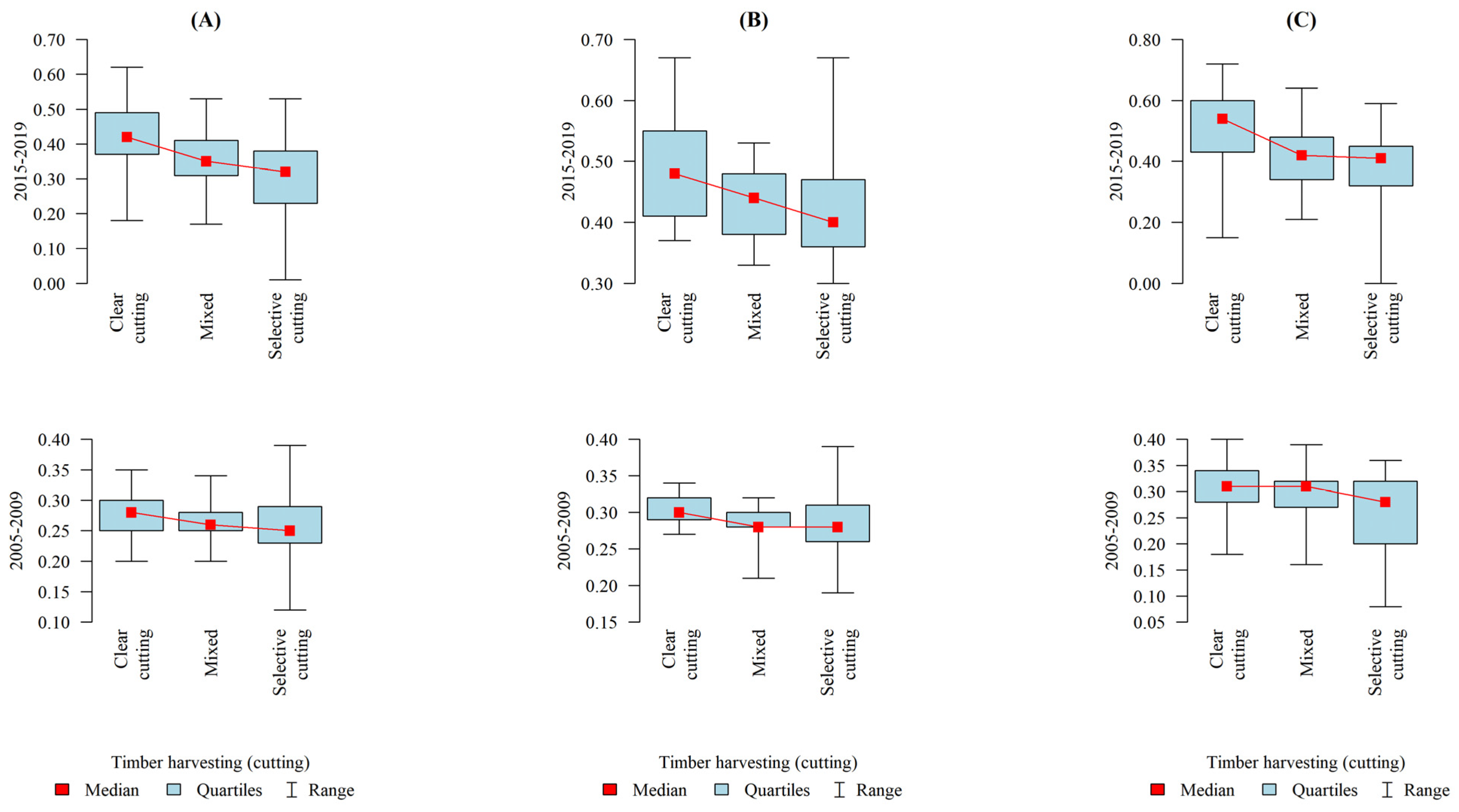
For many years now, stand regeneration systems have been the subject of debate among investors and environmentalists. The study showed that districts with predominant clearcutting were more financially efficient (their synthetic indicators ware significantly higher) as compared to districts with predominant selective cutting. The selection of optimum strategies ranging from continuous regeneration systems to clearcutting is crucial not only from the standpoint of timber production, but also because it has a direct impact on adaptation capacity, biodiversity, as well as esthetic, recreational, and cultural forest functions [36]. Hanewinkel [90] and O’Hara and Ramage [91] noted that economic comparisons between different forest management systems are complicated and poorly understood due to the absence of a framework that would make it possible to accurately describe them and reliably weigh their profitability. Clearcutting has become the most controversial silvicultural practice; also the public often disapproves of the periodical absence of trees and other consequences of clearcutting, such as soil degradation [92]. A study from Alabama shows that while clearcutting is superior in terms of economic efficiency (profitability, worker safety, and organization), it is considered the environmentally damaging [93]. In the present study, the median of the synthetic indicator was the highest for forest districts with the largest proportion of clearcutting, but the greatest interquartile range was found for districts with a predominance of mixed and selective cutting systems. According to Cubbage [94], harvesting costs often surpass actual wood growing costs. Aalmo et al. [95] noted that ineffective harvesting operations can be improved, for instance by raising stand density or by increasing stem-volume for pine trees and broadleaves. Mixed felling systems usually entail higher costs [96]. Thus, efforts should be made to increase the share of cheaper natural regeneration practices in forests, which may be facilitated by diversifying the age structure of stands. Despite the limited possibilities of mechanical harvesting, the costs of planting and tending to the new forest generation are lower in uneven-aged stands because natural regeneration and self-thinning are the central elements of forest management while harvesting focuses on large trees [85].
Forest district revenues are affected by volume of harvested timber, and the structure of assortments produced from that timber. However, no statistically significant differences in financial performance were identified between forest district categories distinguished on the basis of harvesting volume. In 2015–2019 both the means and medians of synthetic indicators 1 and 3 were higher in forest districts characterized by intensive timber harvesting.
As the management of smaller stands entails lower economies of scale and impedes active management [97,98], it was expected that the fragmentation of forest complexes would have an impact on the financial performance of forest districts, but research did not bear out this hypothesis. Kittredge [99] noted that the concentration of forest ownership may bring environmental and operational benefits, e.g., by optimizing and decreasing the number of access roads and skid trails, and thus reducing harvesting costs [81].
This study also analyzed relationships between the synthetic financial indicators and the aggregated management difficulty indicator developed by Kocela et al. [67] using an “aggregate of relative values” expressing the difficulty of conducting forestry operations in individual forest districts [29]. The present findings did not reveal differences between the forest district categories distinguished on the basis of management difficulty and the applied synthetic financial indicators. These results should be treated cautiously as the management difficulty indicators may have already become partially obsolete for the 2015–2019 period (however, no statistically significant relationships were detected in 2005–2009, either).
The synthetic indicator calculated according to the Universal Model (excluding Forest Fund transfers from accounting records) exhibited the lowest mean and median values in both studied periods, being significantly different (p < 0.05) from both the corresponding indicator including Forest Fund transfers and the indicator calculated pursuant to Buraczewski and Wysocki’s model [73]. The novelty of the study consists of applying synthetic indicators calculated on the basis of different methodological assumptions for the evaluation of the financial performance of forest districts operating in different conditions as well as in analyzing the relationship between that performance and selected forest management conditions. The present study showed that a multiplicity of financial ratios can be successfully replaced with one synthetic measure representing the financial performance of forest districts. Furthermore, the use of two variants of accounting records and two sets of financial ratios enabled additional comparisons.
The financial condition of the analyzed forest districts varies and depends on many variables. In addition to the discussed natural and economic factors, it is affected by the increasing costs of nature and biodiversity conservation and the implementation of forest social functions, such as nature education and recreation. The increasing importance of non-production ecosystem services has reduced timber harvesting, especially due to nature conservation and recreational functions. Moreover, weather anomalies have increased forest management costs and uncertainty, thus adversely affecting the profitability of SFNFH holdings.

5. Conclusions

In the years 2015–2019, financial indicators revealed substantial variability and reflected an excessive liquidity of forest districts. A comparison with the findings for 2005–2009 indicated that their current liquidity was lower by approx. 5%. The activity (efficiency) ratios showed a good inventory turnover period as well as a short receivables conversion period. In the study period, the profitability indicators, and in particular ROS and ROE were unfavorable. A comparison of the mean values of those ratios indicates a slight deterioration of financial performance with respect to the period 2005–2009.
The study corroborated the hypothesis that studied natural and economic factors affect the financial performance of forest districts, except for compatibility between stand species composition and FST, management difficulty, and the fragmentation of forest complexes (apart from synthetic indicator 2). Taking into consideration natural factors, especially FST the most beneficial financial results were obtained by forest districts operating on lowland sites, while those operating in montane conditions exhibited the lowest results. In the context of site fertility, the highest values of the synthetic indicators were obtained for forest districts managing sites low in nutrients (coniferous forests). As regards species composition, it was found that the dominance of pine trees in stands was associated with superior financial performance. Among the economic factors, the most pronounced effects were attributable to the felling system (clear-cutting).
The presented models implementing synthetic financial indicators supplement traditional ratio analysis. They provide a single figure for evaluating the financial performance of forest districts as well as for comparing them in a given period. It should be noted that the indicators revealed high variation in the financial performance of forest districts, with their values remaining much below unity.
Synthetic financial indicator 1 (excluding Forest Fund transfers) was significantly lower than indicator 2, which confirms the limited applicability of the latter metric, constructed on the basis of ratios calculated from the balance sheet and profit and loss records of forest districts. In the case of SFNFH units, ratio analysis should not be performed using items from their financial statements, which are distorted by contributions to and subsidies from the Forest Fund.
Findings concerning the effects of selected natural and economic factors on the financial condition of forest districts may be used for financial planning and management by SFNFH, in particular in decision-making processes aimed to optimize forest management. The applied methods may provide the basis for constructing a sectoral evaluation tool.
Numerous factors affect the financial performance of forest districts, and so it is necessary to continue research into the effects of natural conditions, climate warming, economic changes, and ecosystem services (recreation and nature conservation) on that performance. Efforts should be made to develop economically optimal models of forest management for forest districts depending on their production potential, economic conditions, and social needs.

Author Contributions

Conceptualization, A.K. and A.M.; Methodology, A.M. and A.K.; Software, A.K. and A.M.; Validation, A.K. and A.M.; Investigation, A.K. and A.M.; Writing—Original draft preparation, A.K. and A.M.; Writing—Review and editing, A.K. and A.M.; Visualization A.K. and A.M.; Supervision, A.K. and A.M. All authors have read and agreed to the published version of the manuscript.

Funding

This study was financed by The Ministry of Science and Higher Education of the Republic of Poland.

Acknowledgments

We would like to thank the State Forests National Forest Holding for making data available to us. We also thank the three reviewers and editor for the effective feedback provided.

Conflicts of Interest

The authors declare no conflict of interest.

Appendix A

Table A1. Categories of forest districts distinguished due to the percentage share of forest site types (FST).
Category/
N-Number of Forest Districts
I (n = 20)II (n = 20)III (n = 24)IV (n = 9)V (n = 9)Object (n = 82)
FST [%]
FCF33.1912.953.030.620.0012.99
MCF4.290.660.410.000.001.43
FMCF26.6834.9614.301.070.0019.74
MMCF9.774.892.210.320.004.47
FMBF7.0523.1728.772.840.0015.87
MMBF4.303.864.780.240.003.46
BMBF2.572.542.080.000.001.89
FBF2.279.0930.971.850.1611.74
MBF0.871.775.060.160.022.11
ASF3.103.103.510.300.002.60
AASF1.041.632.150.110.011.29
FUBF1.260.001.0972.727.628.22
FMontBF0.000.000.0014.5188.8711.56
Category: I—lowland (coniferous), II—lowland (mixed), III—lowland (broadleaved), IV—upland, V—mountain.
Table A2. Categories of forest districts distinguished on the basis of the fertility of forest site types.
CategoryRange of the Value of the Forest Site Fertility IndexAverage Value for the Category
Values fromValues to
I Very poor (n = 14)2.1712.9462.635
II Poor (n = 27)3.0223.6203.300
III Fertile (n = 21)3.6814.2563.986
IV Very fertile (n = 20)4.5234.9744.857
Total (n = 82)2.1714.9743.694
Table A3. Categories of forest districts distinguished on the basis of compatibility between stand species composition and forest site type.
CategoryNumber of Forest DistrictsThe Range of Indicator Values in the CategoryAverage Index Value in the Category
Values fromValues to
Incompatible22−0.130.890.58
Partially compatible280.941.411.23
Compatible321.441.941.62
Total82−0.131.941.14
Table A4. Categories of forest districts distinguished on the basis of tree species composition.
CategoryNumber of Forest DistrictsVolume Share [%]
PineSpruceFirOakBeech
I (Pine)5085.56.41.15.21.7
II (Oak-pine)963.84.00.029.52.7
III (Pine-spruce)724.166.60.09.30.0
IV (Fir-beech)1617.23.635.22.241.9
Total8262.312.18.37.010.3
Table A5. Categories of forest districts distinguished on the basis of stand regeneration/felling system.
CategoryNumber of Forest DistrictsFelling System [%]
Clear CuttingMixed (Selective)
I (Clear cutting)2674.8225.18
II (Mixed)2145.1354.87
III (Selective cutting)354.7195.29
Total8238.2261.78
Table A6. Categories distinguished on the basis of timber harvesting intensity (per 1 ha of forest area).
CategoryNumber of Forest DistrictsTimber Harvesting Intensity [m3/ha]Average Timber Harvest for the Category
MinimumMaximum
Medium161.283.382.81
High363.424.593.99
Very high304.696.205.22
Total821.286.204.01
Table A7. Categories distinguished on the basis of the fragmentation of forest complexes.
CategoryNumber of Forest DistrictsRange of Values of Land Selection in a Forest DistrictAverage
Values fromValues to
I High411.053.962.55
II Medium294.498.766.18
III Low129.2919.7911.95
Total821.0519.796.89
Table A8. The categories of forest districts distinguished on the basis of the level of difficulty of forest management.
Category of Forest DistrictNumber of Forest DistrictsThe Range of Economic Difficulty for the CategoryAverage
MinimumMaximum
I “Very easy”615.23117.82016.593
II “Easy”2618.93422.29820.715
III “Difficult”3722.42425.98423.956
IV “Very difficult”1326.61131.84628.704
Total8215.23131.84622.492

References

  1. Kangas, J.; Leskinen, P.; Pukkala, T. Integrating timber price scenario modeling with tactical management planning of private forestry at forest holding level. Silva Fenn. 2000, 34, 399–409. [Google Scholar] [CrossRef] [Green Version]
  2. Yousefpour, R.; Jacobsen, J.B.; Thorsen, B.J.; Meilby, H.; Hanewinkel, M.; Oehler, K. A review of decision-making approaches to handle uncertainty and risk in adaptive forest management under climate change. Ann. For. Sci. 2012, 69, 1–15. [Google Scholar] [CrossRef]
  3. Hanewinkel, M.; Cullmann, D.; Schelhaas, M.J. Climate change may cause severe loss in the economic value of European forest land. Nat. Clim. Chang. 2013, 3, 203–207. [Google Scholar] [CrossRef]
  4. Maksymets, O.; Lönnstedt, L. Trends in Markets for Forest-Based Products and Consequences for Selected Countries. Open J. For. 2015, 5, 697–710. [Google Scholar] [CrossRef] [Green Version]
  5. Brecka, A.F.J.; Shahi, C.; Chen, H.Y.H. Climate change impacts on boreal forest timber supply. For. Policy Econ. 2018, 92, 11–21. [Google Scholar] [CrossRef]
  6. Kao, C.J. Measuring the efficiency of forest districts with multiple working circles. J. Oper. Res. Soc. 1998, 49, 583–590. [Google Scholar] [CrossRef]
  7. Młynarski, W.; Prędki, A. Metoda DEA w badaniu efektywności nadleśnictw. Sylwan 2017, 161, 1018–1025. [Google Scholar]
  8. Siry, J.P.; Newman, D.H. A Stochastic Production Frontier Analysis of Polish State Forests. For. Sci. 2001, 47, 526–533. [Google Scholar]
  9. Xiong, L.; Wang, F.; Cheng, B.; Yu, C. Identifying factors influencing the forestry production efficiency in Northwest China. Resour. Conserv. Recycl. 2018, 130, 12–19. [Google Scholar] [CrossRef]
  10. Młynarski, W.; Prędki, A.; Kaliszewski, A. Efficiency and factors influencing it in forest districts in southern Poland: Application of Data Envelopment Analysis. For. Policy Econ. 2021, 130, 102530. [Google Scholar] [CrossRef]
  11. Costa, M.P.; Schoeneboom, J.C.; Oliveira, S.A.; Viñas, R.S.; de Medeiros, G.A. A socio-eco-efficiency analysis of integrated and non-integrated crop-livestock-forestry systems in the Brazilian Cerrado based on LCA. J. Clean. Prod. 2018, 171, 1460–1471. [Google Scholar] [CrossRef] [Green Version]
  12. Pezdevšek Malovrh, Š.; Paletto, A.; Posavec, S.; Dobšinská, Z.; Đorđević, I.; Marić, B.; Avdibegović, M.; Kitchoukov, E.; Stijović, A.; Trajkov, P.; et al. Evaluation of the Operational Environment Factors of Nature Conservation Policy Implementation: Cases of Selected EU and Non-EU Countries. Forests 2019, 10, 1099. [Google Scholar] [CrossRef] [Green Version]
  13. Chen, S.; Yao, S. Evaluation of Forestry Ecological Efficiency: A Spatiotemporal Empirical Study Based on China’s Provinces. Forests 2021, 12, 142. [Google Scholar] [CrossRef]
  14. Brockerhoff, E.G.; Barbaro, L.; Castagneyrol, B.; Forrester, D.I.; Gardiner, B.; González-Olabarria, J.R.; Lyver, P.O.; Meurisse, N.; Oxbrough, A.; Taki, H.; et al. Forest biodiversity, ecosystem functioning and the provision of ecosystem services. Biodivers Conserv. 2017, 26, 3005–3035. [Google Scholar] [CrossRef] [Green Version]
  15. Lundmark, R.; Lundgren, T.; Olofsson, E.; Zhou, W. Meeting Challenges in Forestry: Improving Performance and Competitiveness. Forests 2021, 12, 208. [Google Scholar] [CrossRef]
  16. Maesano, M.; Ottaviano, M.; Lidestav, G.; Lasserre, B.; Matteucci, G.; Scarascia Mugnozza, G.; Marchetti, M. Forest certification map of Europe. iFor.—Biogeosci. For. 2018, 11, 526–533. [Google Scholar] [CrossRef]
  17. Schou, E.; Thorsen, B.J.; Jacobsen, J.B. Regeneration decisions in forestry under climate change related uncertainties and risks: Effects of three different aspects of uncertainty. For. Policy Econ. 2015, 50, 11–19. [Google Scholar] [CrossRef] [Green Version]
  18. Andersson, E.; Keskitalo, E.C.H. Adaptation to climate change? Why business-as-usual remains the logical choice in Swedish forestry. Glob. Environ. Chang. 2018, 48, 76–85. [Google Scholar] [CrossRef]
  19. Neykov, N.; Krišťáková, S.; Hajdúchová, I.; Sedliačiková, M.; Antov, P.; Giertliová, B. Economic Efficiency of Forest Enterprises—Empirical Study Based on Data Envelopment Analysis. Forests 2021, 12, 462. [Google Scholar] [CrossRef]
  20. Kuźma, M. Financial management of State Forests National Forest Holding in relation to challenges of sustainable development of forestry. Optimum 2018, 94, 87–95. [Google Scholar] [CrossRef]
  21. Buraczewski, A.; Jarosz, K. Podstawości i Gospodarki Finansowej w Lasach Państwowych; Wydawnictwo Akademii Rolniczej im. Augusta Cieszkowskiego: Poznań, Poland, 2005; ISBN 8371603770. [Google Scholar]
  22. Li, Y.; Zhang, D. Industrial Timberland Ownership and Financial Performance of US Forest Products Companies. For. Sci. 2014, 60, 569–578. [Google Scholar] [CrossRef] [Green Version]
  23. Adamowicz, K.; Szczypa, P. Możliwości wykorzystania rachunkowości zarządczej w Lasach Państwowych. Pr. Nauk. Uniw. Ekon. We Wrocławiu 2014, 344, 13–24. [Google Scholar] [CrossRef]
  24. Pagde, A.; Kim, Y.; Daugherty, P.J. What Makes Community Forest Management Successful: A Meta-Study from Community Forests throughout the World. Soc. Nat. Resour. 2006, 19, 33–52. [Google Scholar] [CrossRef]
  25. Susaeta, A.; Adams, D.C.; Carter, D.R.; Gonzalez-Benecke, C.; Dwivedi, P. Technical, allocative, and total profit efficiency of loblolly pine forests under changing climatic conditions. For. Policy Econ. 2016, 72, 106–114. [Google Scholar] [CrossRef] [Green Version]
  26. Liubachyna, A.; Bubbico, A.; Secco, L.; Pettenella, D. Management Goals and Performance: Clustering State Forest Management Organizations in Europe with Multivariate Statistics. Forests 2017, 8, 504. [Google Scholar] [CrossRef] [Green Version]
  27. Adamowicz, K.; Gostołek, R.; Jaszczak, R.; Szczypa, P.; Szramka, H. Ocena wpływu wybranych zabiegów hodowlanych i typów siedliskowych lasu na koszt pozyskania surowca drzewnego w czyszczeniach i trzebieżach. Sylwan 2016, 160, 993–1001. [Google Scholar]
  28. Kocel, J.; Kwiecień, R.; Mionskowski, M.; Garbacz, M. Metoda standaryzacji kosztów administracyjnych nadleśnictw z wykorzystaniem stopnia trudności gospodarowania. Sylwan 2017, 161, 226–237. [Google Scholar]
  29. Kocel, J.A.; Kwiecien, R. Metodyczne podstawy określania wskaźnika stopnia trudności gospodarowania leśnictw Lasów Państwowych. Sylwan 2012, 156, 118–127. [Google Scholar]
  30. Petrov, A.P.; Morkovina, S.S. Model of economic organization of the Russian forestry. In IOP Conference Series: Earth and Environmental Science; IOP Publishing: Voronezh, Russian Federation, 2019; Volume 226, p. 12041. [Google Scholar] [CrossRef]
  31. Butler, B.J.; Leatherberry, E.C. America’s family forest owners. J. For. 2004, 102, 4–9. [Google Scholar]
  32. Hatcher, J.; Straka, T.; Greene, J. The Size of Forest Holding/Parcelization Problem in Forestry: A Literature Review. Resources 2013, 2, 39–57. [Google Scholar] [CrossRef]
  33. Knoke, T. Mixed forests and finance—Methodological approaches. Ecol. Econ. 2008, 65, 590–601. [Google Scholar] [CrossRef]
  34. Rämö, J.; Tahvonen, O. Economics of harvesting uneven-aged forest stands in Fennoscandia. Scand. J. For. Res. 2014, 29, 777–792. [Google Scholar] [CrossRef]
  35. Rämö, J.; Tahvonen, O. Economics of harvesting boreal uneven-aged mixed-species forests. Can. J. For. Res. 2015, 45, 1102–1112. [Google Scholar] [CrossRef]
  36. Tahvonen, O. Economics of rotation and thinning revisited: The optimality of clearcuts versus continuous cover forestry. For. Policy Econ. 2016, 62, 88–94. [Google Scholar] [CrossRef]
  37. Davies, S.; Bathgate, S.; Petr, M.; Gale, A.; Patenaude, G.; Perks, M. Drought risk to timber production-A risk versus return comparison of commercial conifer species in Scotland. For. Policy Econ. 2020, 117, 102189. [Google Scholar] [CrossRef]
  38. Polyakov, M.; Wear, D.; Huggett, R. Harvest Choice and Timber Supply Models for Forest Forecasting. For. Sci. 2010, 56, 344–355. [Google Scholar]
  39. Soman, H.; Kizha, A.R.; Muñoz Delgado, B.; Kenefic, L.S.; Kanoti, K. Production economics: Comparing hybrid tree-length with whole-tree harvesting methods. For. Int. J. For. Res. 2020, 93, 389–400. [Google Scholar] [CrossRef]
  40. Callaghan, D.; Khanal, P.; Straka, T.; Hagan, D. Influence of Forestry Practices Cost on Financial Performance of Forestry Investments. Resources 2019, 8, 28. [Google Scholar] [CrossRef] [Green Version]
  41. Garbusewicz, W. Analiza Finansowa Przedsiebiorstwa: Teoria i Zastosowanie; Polskie Wydawnictwo Ekonomiczne: Warszawa, Poland, 2014; ISBN 978-83-208-2086-7. [Google Scholar]
  42. Bednarski, L. Analiza Finansowa w Przedsiębiorstwie; PWE: Warszawa, Poland, 2007; ISBN 83-208-1659-9. [Google Scholar]
  43. Toscani, P.; Sekot, W. Forest Accountancy Data Networks—A European Approach of Empirical Research, Its Achievements, and Potentials in Regard to Sustainable Multiple Use Forestry. Forests 2018, 9, 220. [Google Scholar] [CrossRef] [Green Version]
  44. Dög, M.; Wildberg, J.; Möhring, B. Analysis of a long-term Forest Accountancy Network to Support Management and Controlling. Open Agric. 2018, 3, 155–162. [Google Scholar] [CrossRef]
  45. Lysik, K. Wpływ Warunków Przyrodniczych i Wybranych Czynników Ekonomicznych na Sytuację Finansową Nadleśnictw w RDLP Katowice, Kraków i Krosno. Ph.D. Thesis, Akademia Rolnicza w Krakowie, Kraków, Poland, 2005. [Google Scholar]
  46. Sierpińska, M.; Wędzki, D. Zarządzanie Płynnością Finansową w Przedsiębiorstwie; PWN: Warszawa, Poland, 2010; ISBN 9788301151362. [Google Scholar]
  47. Pomykalska, B.; Pomykalski, P. Analiza Finansowa Przedsiębiorstwa; PWN: Warszawa, Poland, 2007; ISBN 9788301148713. [Google Scholar]
  48. Jachna, T.; Sierpińska, M. Ocena Przedsiębiorstwa Według Standardów Światowych; PWN: Warszawa, Poland, 2004; ISBN 9788301149871. [Google Scholar]
  49. Płotkowski, L. Kluczowe problemy współczesnego leśnictwa. Sylwan 2004, 148, 22–36. [Google Scholar]
  50. Kupcak, V. Elementary financial analysis of the Forests of the Czech Republic, state enterprise. J. For. Sci. 2005, 51, 127–140. [Google Scholar] [CrossRef] [Green Version]
  51. Ankudo-Jankowska, A.; Glura, J. Assessing the usefulness of accounting measures for examining profitability of the State Forests’ National Forest Holding. For. Res. Pap. 2016, 77, 158–165. [Google Scholar] [CrossRef] [Green Version]
  52. Zamula, I.; Tanasiieva, M.; Travin, V.; Nitsenko, V.; Balezentis, T.; Streimikiene, D. Assessment of the Profitability of Environmental Activities in Forestry. Sustainability 2020, 12, 2998. [Google Scholar] [CrossRef] [Green Version]
  53. Czarnecki, J.; Glura, J.; Ankudo-Jankowska, A. Costs of forest district and statutory duties. Acta Sci. Pol.—Silvarum Colendarum Ratio Ind. Lignaria 2016, 15, 215–221. [Google Scholar] [CrossRef]
  54. Bogler, B.; Kerstens, K.; Moesen, W.; Vanneste, J. A non-parametric Free Disposal Hull (FDH) approach to technical efficiency: An illustration of radial and graph efficiency measures and some sensitivity results. Swiss J. Econ. Stat. 1994, 130, 647–667. [Google Scholar]
  55. Kao, C. Efficiency measurement for parallel production systems. Eur. J. Oper. Res. 2009, 196, 1107–1112. [Google Scholar] [CrossRef]
  56. Yang, B.; Zhang, Y.; Zhang, H.; Zhang, R.; Xu, B. Factor-specific Malmquist productivity index based on common weights DEA. Oper. Res. Int. J. 2016, 16, 51–70. [Google Scholar] [CrossRef]
  57. Ustawa z 28 Września 1991 r. o Lasach. Dziennik Ustaw Nr 101: 444, Poland. Parliamentary Act. Available online: https://isap.sejm.gov.pl/isap.nsf/DocDetails.xsp?id=WDU19911010444 (accessed on 9 November 2021).
  58. Rozporządzenie Rady Ministrów z 6 Grudnia 1994 r. w Sprawie Szczegółowych Zasad Gospodarki Finansowej w Państwowym Gospodarstwie Leśnym Lasy Państwowe. Dziennik Ustaw Nr 134: 692, Poland. Parliamentary Act. Available online: http://isap.sejm.gov.pl/isap.nsf/DocDetails.xsp?id=WDU19941340692 (accessed on 9 November 2021).
  59. Zarządzenie nr 78 Dyrektora Generalnego Lasów Państwowych z Dnia 17 Grudnia 2020 r. Zmieniające Zarządzenie nr 76 Dyrektora Generalnego Lasów Państwowych z Dnia 10 Grudnia 2019 r. w Sprawie Wprowadzenia Jednolitego Tekstu Zasad (Polityki) Rachunkowości Państwowego Gospodarstwa Leśnego Lasy Państwowe i Planu Kont z Komentarzem Państwowego Gospodarstwa Leśnego Lasy Państwowe (Znak: EG.0210.4.2019). Legal Act, Poland. Available online: https://sip.lex.pl/akty-prawne/dzienniki-resortowe/zmiana-zarzadzenia-nr-76-dyrektora-generalnego-lasow-panstwowych-z-35845579 (accessed on 9 November 2021).
  60. Ustawa z 29 Września 1994 r. o Rachunkowości, 2013, p. 330 i 613 z Późn. zm. Dziennik Ustaw Nr 121: 591, Poland. Parliamentary Act. Available online: sap.sejm.gov.pl/isap.nsf/DocDetails.xsp?id=wdu19941210591 (accessed on 9 November 2021).
  61. Piekutin, J.; Gruchała, A. Miejsce i rola funduszu leśnego w systemie finansowym Lasów Państwowych. Sylwan 2006, 2, 37–45. [Google Scholar]
  62. Adamowicz, K.; Dyrcz, A.; Szczypa, P.; Zyroń, A.; Michalski, K.; Szramka, H. Wpływ funduszu leśnego na wartość poszczególnych pozycji bilansu finansowego gospodarstwa leśnego. Acta Sci. Pol. Silvarum Colendarum Ratio Ind. Lignaria 2017, 16, 157–164. [Google Scholar]
  63. Piekutin, J. Analiza funkcjonowania funduszu leśnego w systemie finansowym Lasów Państwowych na przykładzie Regionalnej Dyrekcji Lasów Państwowych w Radomiu. Sylwan 2006, 6, 3–18. [Google Scholar]
  64. GUS. Leśnictwo; GUS: Warszawa, Poland, 2016. [Google Scholar]
  65. GUS. Leśnictwo; GUS: Warszawa, Poland, 2020. [Google Scholar]
  66. Kocel, J.; Kwiecień, R.; Młynarski, W.; Mionskowski, M. Wskaźnik stopnia trudności gospodarowani aleśnictw Lasów Państwowych. Sylwan 2012, 156, 403–413. [Google Scholar]
  67. Kocel, J.; Kwiecień, R. Metoda określania syntetycznego wskaźnika efektów gospodarowania zasobami przyrodniczymi, ludzkimi i ekonomicznymi nadleśnictw. For. Res. Pap. 2010, 71, 91–104. [Google Scholar] [CrossRef] [Green Version]
  68. Bansal, A. Improved K-mean Clustering Algorithm for Prediction Analysis using Classification Technique in Data Mining. Int. J. Comput. Appl. 2017, 157, 35–40. [Google Scholar] [CrossRef]
  69. Głaz, J.; Dawidziuk, J. Wytyczne do Sporządzania Aneksu Ekonomicznego do Planu Urządzenia Lasu; Maszynopis: Warszawa, Poland, 2009. [Google Scholar]
  70. Soana, M.G.; Barbieri, L.; Lippi, A.; Rossi, S. The Effect of Multiple Large Shareholders on Banks’ Profitability and Risk. Sustainability 2021, 13, 1888. [Google Scholar] [CrossRef]
  71. Kunca, A.; Zúbrik, M.; Galko, J.; Vakula, J.; Leontovyc, R.; Konôpka, B.; Nikolov, C.; Gubka, A.; Longauerová, V.; Malová, M.; et al. Salvage felling in the Slovak forests in the period 2004–2013. Lesn. Cas. 2015, 61, 188–195. [Google Scholar] [CrossRef] [Green Version]
  72. Zaleska, M. Ocena Ekonomiczno Finansowa Przedsiębiorstwa Przez Analityka Bankowego; SGH: Warszawa, Poland, 2005; ISBN 83-7378-004-1. [Google Scholar]
  73. Buraczewski, A.; Wysocki, F. Ocena sytuacji finansowej nadleśnictw za pomocą syntetycznego miernika rozwoju. Sylwan 2000, 1, 43–52. [Google Scholar]
  74. Kukuła, K. Metoda Unitaryzacji Zerowanej; Wydawnictwo Naukowe PWN: Warszawa, Poland, 2005; ISBN 83-01-13097-0. [Google Scholar]
  75. R Core Team. R: A Language and Environment for Statistical Computing; R Foundation for Statistical Computing: Vienna, Austria, 2021; Available online: https://www.R-project.org/ (accessed on 1 August 2021).
  76. Tyran, M.R. Wskaźniki Finansowe; OE: Kraków, Poland, 2005; ISBN 8389355329. [Google Scholar]
  77. Szymkiewicz, B. Tablice Zasobności i Przyrostu Drzewostanów Ważniejszych Gatunków Drzew Leśnych, Zesta−Wione na Podstawie Tablic Niemieckich, Radzieckich i Polskich; PWRiL: Warszawa, Poland, 1971. [Google Scholar]
  78. Wildberg, J.; Möhring, B. Empirical analysis of the economic effect of tree species diversity based on the results of a forest accountancy data network. For. Policy Econ. 2019, 109, 101982. [Google Scholar] [CrossRef]
  79. Brang, P.; Spathef, P.; Larsen, J.B.; Svoboda, M. Suitability of close-to-nature silviculture for adapting temperate European forests to climate change. Forestry 2014, 87, 492–503. [Google Scholar] [CrossRef] [Green Version]
  80. Hildebrandt, P.; Knoke, T. Investment decisions under uncertainty—A methodological review on forest science studies. For. Policy Econ. 2011, 13, 1–15. [Google Scholar] [CrossRef]
  81. Schulte, A.A.; Rickenbach, M.; Marrick, L.C. Ecological and economic benefits of cross-boundary coordination among private forest landowners. Landsc. Ecol. 2008, 23, 481–496. [Google Scholar] [CrossRef]
  82. Albert, M.; Hansen, J.; Nagel, J.; Schmidt, M.; Spellmann, H. Assessing risks and uncertainties in forest dynamics under different management scenarios and climate change. For. Ecosyst. 2015, 2, 14. [Google Scholar] [CrossRef] [Green Version]
  83. Pukkala, T. Effect of species composition on ecosystem services in European boreal forest. J. For. Res. 2018, 29, 261–272. [Google Scholar] [CrossRef]
  84. Janeczko, K. Ekonomiczne Konsekwencje Realizacji Pozaprodukcyjnych Funkcji Lasu na Przykładzie Leśnego Kompleksu Promocyjnego Puszcza Białowieska. Ph.D. Thesis, SGGW, Warszawa, Poland, 2004. [Google Scholar]
  85. Friedrich, S.; Paul, C.; Brandl, S.; Biber, P.; Messerer, K.; Knoke, T. Economic impact of growth effects in mixed stands of Norway spruce and European beech—A simulation based study. For. Policy Econ. 2019, 104, 65–80. [Google Scholar] [CrossRef]
  86. Knoke, T.; Ammer, C.; Stimm, B.; Mosandl, R. Admixing broadleaved to coniferous tree species: Areviewon yield, ecological stability and economics. Eur. J. For. Res. 2008, 127, 89–101. [Google Scholar] [CrossRef]
  87. Hanewinkel, M.; Frutig, F.; Lemm, R. Economic performance of uneven-aged forests analysed with annuities. Forestry 2014, 87, 49–60. [Google Scholar] [CrossRef] [Green Version]
  88. Knoke, T.; Kindu, M.; Jarisch, I.; Gosling, E.; Friedrich, S.; Bödeker, K.; Paul, C. How considering multiple criteria, uncertainty scenarios and biological interactions may influence the optimal silvicultural strategy for a mixed forest. For. Policy Econ. 2020, 118, 102239. [Google Scholar] [CrossRef]
  89. Knoke, T.; Stimm, B.; Ammer, C.; Moog, M. Mixed forests reconsidered: A forest economics contribution on an ecological concept. For. Ecol. Manag. 2005, 213, 102–116. [Google Scholar] [CrossRef] [Green Version]
  90. Hanewinkel, M. Comparative economicinvestigations of even-aged anduneven-aged silvicultural systems: Acritical analysis of different methods. Forestry 2002, 75, 473–481. [Google Scholar] [CrossRef] [Green Version]
  91. O’Hara, K.L.; Ramage, B.S. The stand: Revisiting a central concept in forestry. J. For. 2013, 111, 335–340. [Google Scholar] [CrossRef] [Green Version]
  92. McCool, S.F.; Benson, R.E.; Ashor, J.L. How the public perceives the visual effects of timber harvesting: An evaluation of interest group preferences. Environ. Manag. 1986, 10, 385–391. [Google Scholar] [CrossRef]
  93. Parmer, A.M.; Gan, J.; Kolison, S. Assessment of the Economic Efficiency and Environmental Impact of Major Timber Harvesting Systems in Alabama. 1999. Available online: https://www.researchgate.net/publication/255626403_Assessment_of_the_Economic_Efficiency_and_Environmental_Impact_of_Major_Timber_Harvesting_Systems_in_Alabama (accessed on 1 August 2021).
  94. Cubbage, F.W. Timber Harvesting. Forest Resource Economics and Policy Research; Routledge: New York, NY, USA, 1989; ISBN 9780429043055. [Google Scholar]
  95. Aalmo, G.O.; Kerstens, P.J.; Belbo, H.; Bogetoft, P.; Talbot, B.; Strange, N. Efficiency drivers in harvesting operations in mixed Boreal stands: A Norwegian case study. Int. J. For. Eng. 2020, 32, 74–86. [Google Scholar] [CrossRef]
  96. Zając, S. Niektóre problemy ekonomiczne gospodarki leśnej w aspekcie reprywatyzacji lasów. Sylwan 1998, 142, 5–16. [Google Scholar]
  97. Greene, J.L.; Blatner, K.A. Identifying woodland owner characteristics associated with timber. management. For. Sci. 1986, 32, 135–146. [Google Scholar]
  98. Munn, I.A.; Barlow, S.A.; Evans, D.L.; Cleaves, D. Urbanization’s impact on timber harvesting in the south central United States. J. Environ. Manag. 2002, 64, 65–76. [Google Scholar] [CrossRef] [PubMed]
  99. Kittredge, D.B. The cooperation of private forest owners on scales larger than one individual property: International examples and potential application in the United States. For. Pol. Econ. 2005, 7, 671–688. [Google Scholar] [CrossRef]
Figure 1. Location of the regional directorates of State Forests in Białystok, Krosno and Lublin.
Forests 12 01559 g001
Figure 2. Ranges, medians, and quartiles of synthetic financial indicators 1, 2 and 3 for forest site types. (A) synthetic indicator 1 calculated for the years 2015–2019 and 2005–2009, (B) synthetic indicator 2 calculated for the years 2015–2019 and 2005–2009), (C) synthetic indicator 3 calculated for the years 2015–2019 and 2005–2009.
Forests 12 01559 g002
Figure 3. Ranges, medians and quartiles of synthetic financial indicators depending on the fertility of forest habitats. (A) synthetic indicator 1 calculated for the years 2015–2019 and 2005-2009, (B) synthetic indicator 2 calculated for the years 2015–2019 and 2005–2009), (C) synthetic indicator 3 calculated for the years 2015–2019 and 2005–2009.
Forests 12 01559 g003
Figure 4. Ranges, medians, and quartiles of synthetic financial indicators 1, 2, and 3 for tree species composition. (A) synthetic indicator 1 calculated for the years 2015–2019 and 2005–2009, (B) synthetic indicator 2 calculated for the years 2015–2019 and 2005–2009), (C) synthetic indicator 3 calculated for the years 2015–2019 and 2005–2009.
Forests 12 01559 g004
Figure 5. Ranges, medians, and quartiles of synthetic financial indicators 1, 2, and 3 for stand regeneration/felling systems. (A) synthetic indicator 1 calculated for the years 2015–2019 and 2005–2009, (B) synthetic indicator 2 calculated for the years 2015–2019 and 2005–2009), (C) synthetic indicator 3 calculated for the years 2015–2019 and 2005–2009.
Forests 12 01559 g005
Table 1. Indicators used in ratio analysis and in developing synthetic indicators.
Universal Model (Used by the SFNFH)CBuraczewski and Wysocki’s Model (2000)C
Current   ratio   ( CR ) = Current   assets Current   liabilities N CR = current   assets current   liabilities N
Quick   ratio   ( QR ) = current   assets     inventory current   liabilities N QR = current   assets     inventory current   liabilities N
Cash   ratio   ( FR ) = short - term   investments   ( cash ) current   liabilities N Debt   ratio   ( DR ) = total   liabilities   ( debt ) total   assets   × 100 % S
Equity   to   fixed   assets   ratio   = ( shareholder   equity   +   non - current   provisions )   fixed   assets S Debt   to   equity ( D E ) = total   liabilities shareholder   equity S
Average collection period (ACP) = average   annual   receivables   ×   365   sales   revenues   ( annual ) D DSI = average   inventory   ×   365 sales   or   COGS D
Days   of   inventory   ( DSI ) = average   annual   inventory   ×   365 sales   or   cost   of   goods   sold D ACP = average   receivables   ×   365 sales   revenues   ( annual ) D
Liabilities   turnover   ratio = average   liabilities   ×   365 net   revenus   from   sales D Return   on   sales   ( ROS ) = net   income   ( net   profit ) ×   100 % sales   revenues S
Return   on   average   assets   ( ROAA ) = net   income   ×   100 % average   total   assets S Return   on   assets   ( ROA ) = net   income   ×   100 % average   current   assets S
Return   on   equity   ( ROE ) = net   income   ×   100 % average   annual   equity S
Note: C—diagnostic variables: N—nominant variables: CR—1.60, QR—1.20, FR—0.20, S—stimulants, D—destimulants.
Table 2. Means, medians, and quartiles for the liquidity, activity, profitability, and debt ratios as well as the financial results of the studied forest districts.
Financial IndicatorPeriod
2015–2019 (n = 82)2005–2009 (n = 82)
Current ratiomean ± SD2.04 ± 1.032.15 ± 0.47
median1.892.05
quartiles1.67–2.161.61–2.5
Quick ratiomean ± SD1.88 ± 0.952.26 ± 2.44
median1.741.96
quartiles1.54–1.991.55–2.31
Cash ratiomean ± SD1.47 ± 0.91.44 ± 0.45
median1.311.37
quartiles1.09–1.61.10–1.71
Equity   to   fixed   assets   ratio [%]mean ± SD101.24 ± 10.92120.93 ± 13.61
median101.43118.79
quartiles94.33–107.3113.47–127.19
Average collection period [days]mean ± SD22.68 ± 27.5213.21 ± 5.66
median14.1113.03
quartiles10.22–24.929.02–17.41
Days   of   inventory   [days]mean ± SD13.15 ± 11.7423.17 ± 116.68
median10.213.14
quartiles8.34–13.649.1–22.02
Liabilities   turnover   ratio [days]mean ± SD25.05 ± 52.6935.15 ± 218.14
median14.1526.5
quartiles11–19.7317.02–36.3
ROS excl. forest fund [%]mean ± SD−5.18 ± 37.89−4.02 ± 14.62
median−0.060.06
quartiles−0.52–6−11.33–5.23
ROA excl. forest fund/(ROA) [%]mean ± SD1.12 ± 10.19 (4.88 ± 3.34)−1.22 ± 12.82 (2.83 ± 2.73)
median−0.03 (3.99)0.5 (2.54)
quartiles−0.28–6.25 (2.34–6.91)−9.46–6.53 (0.84–4.64)
ROE excl. forest fund/(ROE) [%]mean ± SD−3.36 ± 17.73 (4.98 ± 2.79)−1.28 ± 17.64 (3.75 ± 3.53)
median−3.61 (4.38)0.88 (3.27)
quartiles−12.45–7.86 (2.98–6.93)−12.02–7.9 (1.12–6.19)
Debt ratio [%]mean ± SD27.47 ± 5.7814.01 ± 2.21
median26.9214.72
quartiles23.9–30.7613.92–16.18
Debt to equity ratio [%]mean ± SD38.41 ± 11.3420.33 ± 3.8
median3618.6
quartiles31–44.1617.05–22.7
Financial result excl. forest fund [PLN/ha/year]mean ± SD−54.63 ± 239.03−11.17 ± 96.88
median−43.433.97
quartiles−129.65–73.16−50.26–28.73
Table 3. Relationships between the synthetic indicators and forest district categories distinguished on the basis of forest site types.
ParameterForest Site Typep
Lowland Broadleaved—A (n = 24)Lowland Coniferous—B (n = 20)Lowland Mixed—C (n = 20)Upland—D (n = 9)Montane—E (n = 9)
Synthetic indicator 1 (2015–2019)mean ± SD0.33 ± 0.140.38 ± 0.10.42 ± 0.10.33 ± 0.070.23 ± 0.03p = 0.001 *
median0.370.370.420.330.24
quartiles0.25–0.420.34–0.410.37–0.480.32–0.360.21–0.25C > A,D,E
B,A > E
Synthetic indicator 2 (2015–2019)mean ± SD0.45 ± 0.090.44 ± 0.070.48 ± 0.080.42 ± 0.050.36 ± 0.03p = 0.002 *
median0.440.440.480.420.36
quartiles0.38–0.50.39–0.490.42–0.520.39–0.450.34–0.38C,A,B,D > E
Synthetic indicator 3 (2015–2019)mean ± SD0.25 ± 0.480.43 ± 0.120.52 ± 0.120.42 ± 0.060.35 ± 0.06p = 0.002 *
median0.410.420.540.420.32
quartiles0.26–0.470.38–0.490.45–0.590.4–0.440.31–0.38C > B,D,E,A
Synthetic indicator 1 (2005–2009)mean ± SD0.26 ± 0.040.28 ± 0.030.27 ± 0.040.28 ± 0.080.21 ± 0.03p = 0.003 *
median0.260.280.280.280.19
quartiles0.24–0.290.25–0.30.25–0.290.25–0.320.18–0.25B,D,C,A > E
Synthetic indicator 2 (2005–2009)mean ± SD0.28 ± 0.030.3 ± 0.020.3 ± 0.020.3 ± 0.050.26 ± 0.03p = 0.026 *
median0.280.30.290.290.26
quartiles0.27–0.310.28–0.320.28–0.310.28–0.320.23–0.28B,C > E
Synthetic indicator 3 (2005–2009)mean ± SD0.28 ± 0.070.31 ± 0.050.3 ± 0.060.29 ± 0.040.15 ± 0.05p < 0.001 *
median0.290.310.310.290.13
quartiles0.24–0.330.28–0.350.27–0.330.25–0.330.12–0.2B,C,D,A > E
p—Kruskal–Wallis test + post hoc analysis (Dunn test). * Statistically significant (p < 0.05).
Table 4. Relationships between the synthetic indicators and forest district categories distinguished on the basis of site fertility.
ParameterForest Site Fertilityp
Very High—A (n = 20)High—B (n = 21)Low—C (n = 27)Very Low—D (n = 14)
Synthetic indicator 1 (2015–2019)mean ± SD0.28 ± 0.070.33 ± 0.140.38 ± 0.10.45 ± 0.07p < 0.001 *
median0.270.350.370.44
quartiles0.23–0.330.24–0.420.31–0.440.4–0.48D > C,B,A C > A
Synthetic indicator 2 (2015–2019)mean ± SD0.4 ± 0.050.43 ± 0.090.45 ± 0.080.51 ± 0.07p < 0.001 *
median0.390.420.440.51
quartiles0.36–0.430.36–0.480.39–0.510.47–0.55D > C,B,A C > A
Synthetic indicator 3 (2015–2019)mean ± SD0.38 ± 0.080.24 ± 0.520.44 ± 0.120.54 ± 0.1p < 0.001 *
median0.370.410.430.55
quartiles0.32–0.420.26–0.480.39–0.50.49–0.6D > C > A,B
Synthetic indicator 1 (2005–2009)mean ± SD0.24 ± 0.060.26 ± 0.040.27 ± 0.030.27 ± 0.04p = 0.07
median0.240.270.280.28
quartiles0.19–0.270.24–0.290.25–0.290.24–0.29
Synthetic indicator 2 (2005–2009)mean ± SD0.28 ± 0.040.29 ± 0.030.3 ± 0.020.3 ± 0.02p = 0.071
median0.280.280.30.3
quartiles0.25–0.290.28–0.310.28–0.310.28–0.31
Synthetic indicator 3 (2005–2009)mean ± SD0.22 ± 0.080.29 ± 0.070.31 ± 0.050.3 ± 0.07p = 0.002 *
median0.210.310.310.31
quartiles0.15–0.280.27–0.340.28–0.320.26–0.34C,D,B > A
p—Kruskal–Wallis test + post hoc analysis (Dunn test). * Statistically significant (p < 0.05).
Table 5. Relationships between the synthetic indicators and forest district categories distinguished on the basis of tree species composition.
ParameterTree Species Compositionp
Pine—A (n = 50)Pine and Spruce—B (n = 7)Pine and Oak—C (n = 9)Fir and Beech—D (n = 16)
Synthetic indicator 1 (2015–2019)mean ± SD0.39 ± 0.10.25 ± 0.190.36 ± 0.110.27 ± 0.06p = 0.001 *
median0.40.260.360.26
quartiles0.34–0.450.12–0.370.31–0.460.21–0.33A > D,B
Synthetic indicator 2 (2015–2019)mean ± SD0.46 ± 0.080.41 ± 0.080.46 ± 0.060.39 ± 0.05p = 0.005 *
median0.460.380.450.38
quartiles0.39–0.510.36–0.440.44–0.470.36–0.42A,C > D
Synthetic indicator 3 (2015–2019)mean ± SD0.46 ± 0.12−0.13 ± 0.80.4 ± 0.130.38 ± 0.06p = 0.02 *
median0.470.260.390.39
quartiles0.4–0.55−0.66–0.490.32–0.480.33–0.42A > D,B
Synthetic indicator 1 (2005–2009)mean ± SD0.27 ± 0.030.26 ± 0.050.24 ± 0.030.24 ± 0.07p = 0.021 *
median0.280.270.240.25
quartiles0.25–0.290.25–0.290.23–0.250.19–0.27A > D,C
Synthetic indicator 2 (2005–2009)mean ± SD0.3 ± 0.020.28 ± 0.040.28 ± 0.020.27 ± 0.05p = 0.01 *
median0.30.280.280.27
quartiles0.28–0.310.28–0.30.27–0.290.24–0.29A > C,B,D
Synthetic indicator 3 (2005–2009)mean ± SD0.3 ± 0.060.27 ± 0.090.26 ± 0.060.22 ± 0.08p = 0.002 *
median0.310.30.280.22
quartiles0.28–0.340.25–0.310.23–0.290.13–0.28A > C,D
p—Kruskal–Wallis test + post hoc analysis (Dunn test). * Statistically significant (p < 0.05).
Table 6. Relationships between the synthetic indicators and forest district categories distinguished on the basis of stand regeneration/felling system.
ParameterStand Regeneration/Felling Systemp
Clearcutting—A (n = 26)Mixed—B (n = 21)Selective Cutting—C (n = 35)
Synthetic indicator 1 (2015–2019)mean ± SD0.42 ± 0.110.35 ± 0.090.3 ± 0.12p = 0.001 *
median0.420.350.32
quartiles0.37–0.490.31–0.410.23–0.38A > B,C
Synthetic indicator 2 (2015–2019)mean ± SD0.48 ± 0.080.43 ± 0.060.43 ± 0.09p = 0.012 *
median0.480.440.4
quartiles0.41–0.550.38–0.480.36–0.47A > B,C
Synthetic indicator 3 (2015–2019)mean ± SD0.5 ± 0.140.42 ± 0.110.29 ± 0.4p = 0.001 *
median0.540.420.41
quartiles0.43–0.60.34–0.480.32–0.45A > B,C
Synthetic indicator 1 (2005–2009)mean ± SD0.27 ± 0.040.26 ± 0.030.25 ± 0.05p = 0.201
median0.280.260.25
quartiles0.25–0.30.25–0.280.23–0.29
Synthetic indicator 2 (2005–2009)mean ± SD0.3 ± 0.020.28 ± 0.030.28 ± 0.04p = 0.013 *
median0.30.280.28
quartiles0.29–0.320.28–0.30.26–0.31A > B,C
Synthetic indicator 3 (2005–2009)mean ± SD0.3 ± 0.060.29 ± 0.050.25 ± 0.08p = 0.046 *
median0.310.310.28
quartiles0.28–0.340.27–0.320.2–0.32A > C
p—Kruskal–Wallis test + post hoc analysis (Dunn test). * Statistically significant (p < 0.05).
Table 7. Relationships between the synthetic indicators and forest district categories distinguished on the basis of timber harvesting intensity.
ParameterTimber Harvesting Intensityp
Very High—A
(n = 30)
High—B
(n = 36)
Medium—C
(n = 16)
Synthetic indicator 1 (2005–2009)mean ± SD0.29 ± 0.040.25 ± 0.050.25 ± 0.04p = 0.003 *
median0.280.250.26
quartiles0.26–0.310.22–0.280.23–0.28A > C,B
Synthetic indicator 2 (2005–2009)mean ± SD0.3 ± 0.030.28 ± 0.030.28 ± 0.03p = 0.001 *
median0.310.280.28
quartiles0.29–0.320.26–0.30.28–0.31A > C,B
Synthetic indicator 3 (2005–2009)mean ± SD0.31 ± 0.060.26 ± 0.070.26 ± 0.08p = 0.002 *
median0.310.270.29
quartiles0.28–0.350.21–0.310.21–0.33A > C,B
p—Kruskal–Wallis test + post hoc analysis (Dunn test). * Statistically significant (p < 0.05).
Table 8. Relationships between the synthetic indicators and forest district categories distinguished on the basis of the fragmentation of forest complexes.
ParameterFragmentation of Forest Complexesp
High—A
(n = 12)
Medium—B
(n = 29)
Low—C
(n = 41)
Synthetic indicator 1 (2015–2019)mean ± SD0.36 ± 0.110.37 ± 0.10.34 ± 0.13p = 0.517
median0.340.370.33
quartiles0.31–0.430.33–0.450.25–0.42
Synthetic indicator 2 (2015–2019)mean ± SD0.48 ± 0.090.46 ± 0.070.42 ± 0.08p = 0.021 *
median0.450.460.4
quartiles0.42–0.570.39–0.510.36–0.47A,B > C
Synthetic indicator 3 (2015–2019)mean ± SD0.38 ± 0.110.44 ± 0.110.36 ± 0.4p = 0.442
median0.420.430.44
quartiles0.32–0.450.39–0.530.32–0.54
p—Kruskal–Wallis test + post hoc analysis (Dunn test). * Statistically significant (p < 0.05).
Table 9. Relationships between the synthetic indicators and forest district categories distinguished on the basis of management difficulty.
ParameterManagement Difficulty Levelp
“Very Difficult”—A
(n = 13)
“Difficult”—B
(n = 37)
“Easy”—C
(n = 26)
“Very Easy”—D
(n = 6)
Synthetic indicator 1 (2015–2019)mean ± SD0.29 ± 0.120.37 ± 0.120.38 ± 0.10.34 ± 0.02p = 0.063
median0.240.380.380.34
quartiles0.21–0.30.32–0.450.33–0.420.33–0.35
Synthetic indicator 2 (2015–2019)mean ± SD0.39 ± 0.060.46 ± 0.090.45 ± 0.070.45 ± 0.07p = 0.031 *
median0.380.440.450.44
quartiles0.34–0.420.4–0.540.39–0.50.39–0.5B > A
Synthetic indicator 3 (2015–2019)mean ± SD0.39 ± 0.120.42 ± 0.20.45 ± 0.130.39 ± 0.03p = 0.208
median0.340.440.460.39
quartiles0.31–0.480.38–0.520.41–0.530.37–0.41
p—Kruskal–Wallis test + post hoc analysis (Dunn test). * Statistically significant (p < 0.05).
Table 10. Differences in synthetic indicators between 2015–2019 and 2005–2009.
Synthetic Indicator ValueSynthetic Indicator 1 (2015–2019)Synthetic Indicator 2 (2015–2019)Synthetic Indicator 3 (2015–2019)p
mean ± SD0.35 ± 0.120.44 ± 0.080.39 ± 0.29p < 0.001
median0.360.440.42
quartiles0.27–0.430.38–0.490.34–0.52SI2, SI3 > SI1
Synthetic Indicator ValueSynthetic Indicator 1 (2005–2009)Synthetic Indicator 2 (2005–2009)Synthetic Indicator 3 (2005–2009)p
mean ± SD0.26 ± 0.050.29 ± 0.030.28 ± 0.07p < 0.001
median0.270.290.3
quartiles0.24–0.290.28–0.310.24–0.33SI2, SI3 > SI1
p—Friedman test + post hoc analysis (Wilcoxon paired tests with Bonferroni correction).
Publisher’s Note: MDPI stays neutral with regard to jurisdictional claims in published maps and institutional affiliations.

