BIM-Based Co-Simulation of Fire and Occupants’ Behavior for Safe Construction Rehabilitation Planning

Abstract

Construction renovation projects increase the risk of structural fire, mostly due to the accumulation of combustible construction materials and waste. In particular, when the building remains operational during such projects, the redistribution of occupants and interruptions with access corridors/exit egress can exponentially increase the risk for the occupants. Most construction projects are, however, planned and scheduled merely based on the time and budget criteria. While safety is considered paramount and is meant to be applied as a hard constraint in the scheduling stage, in practice, safe evacuation considerations are reduced to rules of thumb and general code guidelines. In this paper, we propose simulation as a tool to introduce safety under structural fire, as a decision criterion, to be mixed with time and budget for selecting the best construction schedule alternative. We have used the BIM (building information model) to extract the building’s spatial and physical properties; and have applied co-simulation of fire, through computational fluid dynamics (CFD), and occupants’ evacuation behavior, through agent-based modeling (ABM) to estimate the average and maximum required safe egress time for various construction sequencing alternatives. This parameter is then used as a third decision criterion, combined with the project’s cost and duration, to evaluate construction schedule alternatives. We applied our method to a three-floor fire zone in a high-rise educational building in Montreal, and our results show that considering the fire safety criterion can make a difference in the final construction schedule. Our proposed method suggests an additional metric for evaluating renovation projects’ construction plans, particularly in congested buildings which need to remain fully or partially operational during the renovation. Thus, this method can be employed by safety officers and facility managers, as well as construction project planners to guide accounting for fire incidents while planning for these types of projects.

1. Introduction

According to the US National Fire Protection Association (NFPA), local fire departments have reported an annual average of 3840 and 2580 structural fire incidents for under construction or renovation sites, respectively. These fires collectively caused 12 civilian deaths, 101 civilian injuries, and $408 million damage in direct property annually between 2013 and 2017 [1]. According to the Canadian Fire Safety Association (CFSA) report published in 2014, the Ontario Fire Marshal (OFM) reported that the total number of fire incidents in occupied buildings under renovation was five times higher than new/vacant buildings under construction. In addition, between 2008 and 2013, fire incidents in renovation projects have increased, despite the reduction in the total number of fires [2]. Renovation construction projects always have the challenge to execute the works on time and within budget, while providing a safe work environment for the workers and the occupants alike. The building is at its most precarious state when construction is scheduled during normal operation conditions. Construction operations limit (or block) access to some areas and redirect the traffic flow and typical routes. The occupants during this time will be unfamiliar with the building’s access and egress. This magnifies the risks of injuries and fatalities during evacuation in buildings, particularly with high vertical and horizontal occupant density [3]. On the other hand, construction activities accumulate combustible waste and could have hazardous operations such as hot work and welding [4]. These act as potential ignition sources increasing the risk of fires with varying intensities. When coupling these risks together, along with those of fires, the probability of civilian casualties and injuries increases dramatically. Accordingly, construction renovation projects carried out during normal operational hours require more complex planning since they must consider the additional risks to keep the occupants safe and minimize their interruption, all while maintaining the project within the time and budget constraints.

This indicates the importance of fire-related safety planning in occupied high-rise buildings that undergo construction renovation. Necessary safety assessments and fire risk mitigation analyses must be conducted in such cases and must be integral metrics for evaluating corresponding proposed construction plans. Popular planning guidelines in the market, such as “The Defense Contract Management Agency of U.S Government (DCMA)” and “The Government Accountability Office (GAO)”, are not designed to evaluate the plans for these types of renovation projects [5]. The question is how the threat and risk of fire during the planning stage can be identified and how this assessment can be used to evaluate the proposed construction plan, in addition to the other evaluation metrics such as time, and cost. To address the proposed argument, various investigations on human evacuation in fire emergencies are required. While the use of Internet of Things (IoT) and sensory data is proposed for tracking and monitoring occupant’s evacuation behavior [6], in the real world, there are not many chances for collecting the required data associated with evacuation time or human behavior in the process of evacuation during an actual fire. That is where software simulation can be helpful to model the behavior of the facility, occupants, and the fire under various scenarios [7]. Accordingly, this paper provides an understanding of the associated fire and evacuation risks related to various construction renovation scenarios in buildings under operation. The approach is implemented by using a building information modeling (BIM) environment and co-simulation of fire and occupant’s behavior in evacuation. Consequently, the best renovation sequencing option will be selected based on three criteria, i.e., fire safety, construction time, and cost at the same time. The paper is organized as follows; a review of the relevant literature on fire, evacuation safety, and construction schedule evaluation will be first provided. Then, the proposed framework for schedule evaluation considering time, cost, and safety will be introduced and implementation of the framework on a case study of an educational building will be presented. Finally, the results are discussed, and conclusions are drawn to provide a set of recommendations as well as suggestions for future work.

2. Previous Studies

Evaluating a renovation plan based on the occupants’ evacuation under fire conditions requires the modeling of fire and evacuation, both separately and together, as well as a method to assess the evacuation performance under a fire incident. Accordingly, this section provides an overview of each of these topics throughout the previous studies. The literature review is designed to highlight the previous works and set the scope and assumptions for this research.

2.1. Fire Modeling and Simulation

Fire incidents have been simulated in four different ways. The first approach is only considering the impact of fire as an exit door closure, rather than modeling the fire itself. G. N. et al. (2019) investigated the impact of such closure probability of exit doors on safe exit evacuation time on the 10th floor of an educational building at USCI. The results showed the importance and criticality of the fire location in front of the exit door. However, this approach did not model the impact of fire and its byproducts such as heat, toxic gases, and visibility reduction on evacuees’ behavior and corresponding impacts on the evacuation time [8]. Alternatively, the second method which models compartment fires is an analytical approach. In this method, which is considered as the simplest, by utilizing a fundamental series of expressions associated with the fire physicochemical processes e.g., Lawson and Quintiere’s computational technique and Alvares and Fernandez-Pello’s empirical model, the fire development can be modeled [9,10,11]. Analytical models are the baseline for the more complex and computer-based methods. Zone and field models, which are the third approach, are from this group. A zone model initially divides a partially enclosed room’s space into two sections with a layer which is a separation of upper hot layer (smoke) and bottom cold layer (air). Additionally, the area of interest is defined as a combination of uniform described zones. In each of these zones, specific mathematical equations describe the conditions of interest. Consolidated Fire and Smoke Transport (CFAST) developed by the National Institute of Standards and Technology (NIST) is a method based on the concept of zonal model and the output of its simulation shows acceptable results, however, the accuracy decreases in models with complex geometry, or when the enclosure is small or the surface is not uniform. Lastly, is the approach that uses computational fluid dynamics (CFD) principles to model the behavior of fire and its byproducts (which is called a field model). Similar to the zonal approach, this model divides an enclosure into smaller zones, but in a larger number, compared to the zone model and simulates fire through numerically solving Navier–Stokes equations for low-speed flows in 3D. Examples of commercial software which operate based on CFD principles (creating field models) are JASMINE, SOFIE, and Fire Dynamic Simulator (FDS) [7,12,13,14,15]. The FDS also provides operators with modeling facilities’ geometry, objects, materials, and fire properties in a programming environment. The simulation results will be obtained in 2D, i.e., plot time history results and slices; as well as 3D, i.e., visual smoke view videos [16,17]. However, using field models requires a tremendous effort to set up and also simulation time is significantly longer than the previous approaches e.g., hours and days of simulation [14].

Working with FDS and its programming interface is challenging due to the limited visualization capacity, specifically to model complex geometries [16,18]. To bridge this gap, a graphical user interface (GUIs), named Pyrosim, is developed to support modeling the facility’s geometry, and simulate the fire in a visual FDS-based environment. This allowed for better measurement of location, temperature, and CO concentration of smoke and visibility reduction produced by fire [13,18,19,20].

2.2. Evacuation Modeling

Agent-based simulation has been used as an established approach for evacuation modeling [18,21] among others. Agent-based modeling (ABM) is a simulation method based on entities as agents [22]. The individual agents behave based on set rules, as well as interactions with other agents, and the environment [18]. While the utilization of ABM has been common in the previous works, a few studies modeled the evacuation without any simulation. For instance, the evacuation Cao et al. (2013) relied on formulas and calculations based on the model with smoke effect and blind evacuation strategy (SEBES) [7]. In that study, the focus of the model was more on characteristics and the location of the fire, as well as the exit door’s width that was inversely proportional to the evacuation time [7]. However, the model was not complex and was unable to consider factors such as velocity changes and the agent’s behavior variations in the fire emergency. Eftekharirad, et al. (2019) combined ABM with an FDS based engine to study the evacuation behavior of residents under a structural fire, in a construction renovation project [21]. That study partially considered some of the effects of fire products on agents’ behavior and also modeled agents for occupants with disabilities.

Several software tools are commercially available to apply ABM for evacuation simulation; including Pathfinder, Anylogic, STEPS, and Evac [23,24,25,26]. WSP’s study in 2017 analyzed three different evacuation software tools, i.e., Pathfinder, Evac, and STEPS. The comparison indicates that the complex geometries are best supported by Pathfinder and STEPS with a satisfying visualization [12]. However, STEPS has difficulty in non-horizontal modeling and FDS geometries are not perfectly coordinated. The Evac also has limited support for complex geometries. The whole study did not address the interaction between agents and smoke, which could influence the evacuation time [12]. Sun and Turkan (2020) modeled the evacuation of a single-story nightclub through ABM, using Anylogic software tool [18]. The critical factors affecting the fire and evacuation in this study were human behavior, physical characteristics of the building, and fire condition [18]. The computational time was reported to be very high, so the authors had to compromise on the model resolution.

On the other hand, considering the vertical load on the evacuation is critical and it is key to have realistic results [18]. In none of the studies by Sun and Turkan (2020), Cao, et al. (2013), Eftekharirad, et al. (2019), and Wang et al.’s (2015) multi-story buildings were modeled, hence the vertical load was not being considered. In Li et al. (2018) [19] and G.N et al. (2019) [8] research, the vertical evacuation was considered, but the fatigue, group movement, and the movement of disabled people in vertical corridors were not competently investigated. On the other hand, based on SFPE human behavior handbook, agents of different ages and gender could have different speeds [27]. Wang et al.’s (2015) study did not consider human characteristics, which are the main contributing factors [20]. Human profiles control the speed, age, size, and height of agents and the behavior dictates the way the agent behaves during the evacuation. Wang et al. (2015) did not differentiate, in terms of speed, between various agents’ profiles and considered one constant speed walk and flow rate [20]. G.N et al.’s (2019) model was also based on a constant velocity with no consideration of age, disability, and genders [8]. Cao et al.’s (2013) model had two velocities for slow and fast pedestrians [7]. Li et al. (2018) provided the profile of young males and females by modeling only one default speed as 1.19 m/s [19]. Considering different speeds for different ages and genders increases the accuracy of the result.

2.3. Fire Evacuation Risk Assessment

Methods used in the literature for the risk assessment of structural fire closely depend on the modeling approach adopted for the fire. For instance, in G.N et al.’s (2019) study that instead of directly modeling the fire, exit blockage was considered; the risk of fire was assessed based on the reduction of safe exits in the building layout during the evacuation [8]. Other approaches considered modeling more of the fire characteristics and incorporating them into the risk assessment model [28]. Generally, fire risk assessment considers two parameters: required safe egress time (RSET) and available safe egress time (ASET). RSET is defined as the physical movement time of the agent to reach a safe area. ASET is the time which incapacitation is predicted for the agent due to the exposure of the agent to the fire products such as smoke. The RSET could be calculated in evacuation software tools and ASET is an output of the FDS or other available tools with the evacuation scenario [13,18,19,20,29].

Wei and Wang (2016) estimated the danger time by considering 2.0 m flue gas height factor from the floor level [13]. Wang et al. (2015) used multiple parameters based on the Society of Fire Protection Engineers (SFPE) handbook. This handbook provides three tolerance limits for agents, i.e., temperature more than 60 °C; carbon monoxide concentration higher than 1400 ppm; and visibility less than 2.0 m. The ASET in this study was when the agent reached visibility of less than 2.0 m [20]. Li et al. (2018) expanded the list of tolerance limits by adding a ‘fractional effective dose’ (FED) parameter in their investigation. They considered a building unsafe if the evacuation time exceeded RSET in which FED value is 0.1 [19]. Implementation of this parameter was based on equations of the SFPE Handbook for the concentration of CO, CO₂, and O₂ [30]. In these two studies, only one level of risk associated with fire was defined which does not show other stages of the evacuation where it involves injured occupants [19].

Sun and Turkan (2020) provided three stages for ASET. The first and second stages are defined based on the height of the smoke layer when it reaches 1.5 m and 1.2 m from the floor level, respectively. The last stage is assigned to the condition where one of the fire reaction byproducts (i.e., heat, toxic gases, or smoke density) reaches the human’s physical tolerance [18]. After running simulations, ASET stages are checked for the uninjured escape, injured escape without death, and failure escape alive, respectively. The output of the evacuation analysis and the building properties were taken into a linear regression model by Sun and Turkan (2020), to compare the required time of evacuation from the building and the available time of evacuation in different conditions [18].

Table 1. Most recent works for fire/evacuation co-simulation.

Author (Year)	Simulation Purpose	Simulation Method	Simulation Tool	Impact of Fire on Evacuation	Vertical/Horizontal Modeling
Mirhadi et al. (2019) [31]	Evaluating fire-related safety of evacuation in a two-story office building by considering the distance of agents from fire and safe evacuation.	A 6-step framework (EvacuSafe) including BIM, Fire Simulation Module, Path Identification Module, Agent-Based Crowd Simulation Module, Calculation of Risk Indices, and Analysis of Design Scenario	• Fire: CYPECAD MEP (FDS) • Evacuation: MassMotion	Defining open/close schedules of gates for affecting the flow because of fire influence on agents’ behavior	Horizontal and Vertical
Ronchi et al. (2019) [32]	A complex agent-based evacuation simulation using a simplified egress model and the smoke-filled portions	A multi-model approach including Basic Assumptions (Fire design, Design behavioral scenario, and Boundary conditions); 1D Smoke Propagation (Visibility) and Toxic Species; Simplified Egress Modeling (in smoked filled areas); Arrival Times to Smoke-free Areas; Advanced Egress Modeling (in complex spaces); and Safe Area	• Fire: FDS • Evacuation: Pathfinder (ABM)	Smoke effect on visibility and speed of occupants	Only Horizontal
Li et al. (2020) [19]	Introducing a method, called FREEgress (Fire Risk Emulated Environment for Egress) to evaluate the impact of three factors: initial fire location; evacuation delay time; and occupants’ behavior) on evacuation process	Generating 30 scenarios based on the initial location of the fire, delay time, and behavior type; Then modeling and running the simulation in the associated software tools	• Fire: Pyrosim • Evacuation: FREEgress (developed based on the SAFEgress software tool)	Impact of fire temperature, toxic gases, and smoke on occupants’ physiology (motion speed and health) and navigation strategy	Only Horizontal
Q. Sun and Y. Turkan (2020) [18]	Developing a BIM Based framework and implementing FDS and ABM for simulation of fire propagation and evacuation performance	(i) A linear regression between the building design and RSET; (ii) Finding the relationship between the fire growth rate and NFH; and (iii) evaluating the effects of designed model parameters by applying two sample t-tests	• Fire: Pyrosim (FDS) • Evacuation: Anylogic (ABM)	Finding effective escape routes as recommended by evacuation scenarios and hazardous zones as reflected in fire simulation	Only Horizontal
Eftekharirad, et al. (2019) [21]	Studying the impact of temporary repurposing and changing the layout due to construction, on the fire and evacuation behavior	Using a co-simulation of the fire propagation and agents’ evacuation under the physical constraints of the construction project	• Fire: Pyrosim (FDS) • Evacuation: Pathfinder (ABM)	Temporary blockage of access due to construction and exit blockage due to fire	Only Horizontal
Gerges et al. (2021) [33]	Develop a BIM Based platform combined with ABM and FDS and sending instructions to the smartphones to improve evacuation from high-rise residential buildings	Using BIM to identify agents’ locations to send them evacuation instructions and simulate them in evacuation software under various scenarios; Then, comparing the regular evacuation time with the constraint evacuation time to evaluate the impact of sending instructions, on the process	• Evacuation: Pathfinder (ABM)	No impact of fire; rather studied the influence of sending instructions to smartphones during the evacuation	Horizontal and Vertical (11-story)
Wang et al. (2021) [34]	Risk evaluation of underground facilities through a proposed risk-assessment method associated with evacuation in fire	Selecting the most likely ignition source of fire by the proposed ‘multi-exit fire-location-selection method’; Then estimating ASET and RSET as inputs for risk assessment. Calculating associated risk with each area and exit route; Finally, evaluating the overall risk of the entire facility	• Fire: Pyrosim • Evacuation: Pathfinder	Considering the CO concentration and outside temperature caused by fire but not directly in the simulation	Horizontal and Vertical

presents a summary of the recent applications similar to the approach taken in the present study. Regardless of the studies’ scope and method, to our best understanding, no researcher has integrated, to date, the fire/evacuation analysis with construction planning, and this has remained a gap in the literature. Accordingly, we use ASET and RSET as the two outputs from fire and evacuation modeling and assess the renovation construction schedule. ABM and FDS will be used through Pathfinder and Pyrosim, which are integrated with the BIM to co-simulate the fire products’ impact, occupants’ evacuation, and the impact of construction operations sequence on the two.

3. Methodology

As mentioned earlier, the main target of the paper is to create a feedback loop between evacuation under fire hazards and the planning process of construction renovation activities. Accordingly, Figure 1 shows the high-level framework implemented in this study, which comprises five main steps, i.e., (1) Building examination; (2) Construction scope definition and planning; (3) Fire Modeling and Simulation Analysis; (4) Evacuation modeling and Co-Simulation; and (5) Construction schedule evaluation. In the following, these steps are explained under three major steps, i.e., preparation; simulation; and evaluation.

3.1. Preparation Phase—Building Examination and Construction Scope Definition and Planning

During building examination, a BIM is used to extract the required information including floor layout; functionality and area of spaces; connections such as corridors and stairs; the number and location of pressurized exit doors; components’ material; fire zones; occupants’ count and density at normal operation; etc. During the construction scope definition and planning, renovation activities and necessary resources i.e., labor, materials, and equipment, are determined based on the types of renovation activities. The planning process uses the output of the building examination for each activity separately to provide insight to (i) the alternative routes in/out of the building for material transfer/debris removal, etc., with minimal interruption to the occupants; (ii) the hazardous tasks within the activity which might require additional measurements to execute them during normal building operations; (iii) alternative occupant reallocation plans (if any) during the project execution; and (iv) the different crew compositions, productivity and associated costs to complete the activity considering the type(s) of interruption happening with each (sound levels, crew movements, etc.)

Afterward, activity relations and dependencies are evaluated to develop the construction plan and that is where the complexity appears. The planner is expected to develop the schedule not only based upon the typical construction logic but also to consider how the activities’ execution would affect/risk the occupants at any point in time. This additional criterion usually could define soft dependencies in a schedule. The soft dependencies between activities are when there is no physical (hard) constraint that dictates their execution order sequence; rather, the planner creates these soft dependencies to streamline the workflow on-site and to level the project resources. Hence, these soft dependencies are re-engineered now to consider occupant interruption and associated risks. Accordingly, multiple schedule alternatives would be developed where the work breakdown, the sequence of operation, activity duration, and critical path are defined in each. Finally, by reviewing the 4D model for each schedule alternative, the planner can define the workspace requirements and generate a snapshot at each unique time interval. These snapshots would resemble the space allocation, the blocked exits, obstructed routes, and shifted occupant density (due to relocation) at any point of the construction schedule. These snapshots are then used in the fire/evacuation modeling.

3.2. Simulation Phase—Fire Modeling and Evacuation Co-Simulation

The building examination outputs and the expected workspace snapshots from the alternative plans, provide the layout for the co-simulation for fire and evacuation. The fire simulation stage comprises the following steps: (i) determining the possible critical fire locations; and (ii) defining the fire characteristics and intensities. The suggested tool for the fire simulation is Pyrosim 2020.1 [17]. According to the previous studies, fire locations in front of exit doors are deemed more critical, and thus should be modeled [13,18,19,20,29]. The fire properties are based on the SFPE Handbook of Fire Engineering Protection by selecting from the materials defined in the project [35]. The fires are modeled in the Pyrosim software tool through the following steps: (a) defining meshes; (b) defining reactions; (c) defining fire ignition source by creating obstruction, material and burner surfaces; (d) defining 2D slices for extracting the fire result; and (e) choosing the simulation time. The results obtained are Pyrosim file (.psm) and smoke view file (.smv) which are required for evacuation modeling and co-simulation.

As prior investigations have implemented the method of evacuation modeling by the help of software tools, in this study, Pathfinder an evacuation simulation software tool is chosen to model the evacuation scenarios [13,18,19,20,29,30]. The fire simulation outputs are imported into Pathfinder. The construction snapshots and occupants’ properties and reallocation plans are used as the basic information of the modeling. To model the evacuation in Pathfinder software tool, the first step is floor extraction and door detection, the second step is creating the occupants based on 2 criteria, the fixed characteristics as profile such as speed, gender, height, and behavioral actions such as waiting and moving toward the exit doors. To couple the Pyrosim (FDS fire result) and Pathfinder, the automatic method is used. The only impact of fire in this co-simulation on evacuation is slowing down the agents by applying a speed factor on the speed of agents due to the deduction of visibility range caused by smoke.

3.3. Evaluation Phase—Construction Schedule Assessment

In the last phase of the method, the construction schedule alternatives are evaluated based on three criteria, i.e., cost (total budget), time (project duration), and safety under fire evacuation. The project duration metric eliminates longer construction plans, which indicate an extended period of interruption to the building’s normal operations. The construction cost metric reviews the overall construction cost and daily cashflow, to ensure the project remains affordable, with the increased safety and logistics parameters. For the occupants’ safety metric, two parameters are considered. First and foremost is the possibility of fatality and casualties. This is being considered as a hard constraint, hence those schedule scenarios that can have the possibility of fatalities will be eliminated. Afterward, a comparison between the RSET with and without fire for each scenario is made and the difference in time is considered as the added risk of evacuation due to the fire. The metrics are coupled to determine the preferred construction scenario.

4. Case Study

In this section, the proposed modeling framework is applied to the actual case study of an educational building. The BIM of a high-rise building located in Concordia University downtown campus, built in 2005 was built and different fire scenarios under renovation alternatives were examined. The modeling process was done on a platform with an Intel dual-core i5 processor (2.5 GHz) with 8 GB available RAM and the simulations were completed on a computer with an Intel quad-core Xenon processor E5 v5 family with 32 GB RAM. The simulation times for modeling different fire scenarios () in Pyrosim ranged from 7.5 h to 13 h, with an average of 10.5 h. The co-simulation times for modeling the evacuation process for the 18 snapshots under each fire scenario () ranged from 263 s to 715 s, averaged around 400 s. Details of the fire scenarios, schedule snapshots, and their combinations are explained later in this section.

4.1. Building Examination and Scope Definition

The case study building comprised two 17-story towers, which are connected through indoor common corridors and include administrative offices, over 300 specialized labs, conference and meeting rooms, some classes and student common areas. Under normal operations, the building has an average of 1000 occupants per day and operates 24 h, 7 days a week. The authors acquired the BIM of the 9th floor, shown in Figure 2 and regenerated the rest of the building. This layout is divided into 2 parts: on the bottom (E-Block) and on top (V-Block). The floor includes six (6) dry laboratories, 35 student offices, nine (9) staff offices, one kitchenette, four bathrooms, eight elevators, and four (4) pressurized exit doors. Every three floors of this building are openly connected in the vertical direction (referred to, as ‘vertical campus’) through two staircases; one spiral staircase in the E-Block, and one regular staircase in the V-Block. According to the fire design of the building, these three vertically connected floors are considered as one fire zone, which seals off fire and smoke from traveling to other floors. Accordingly, the building model was created at two levels of development (LOD): The fire zone which comprised floors 8 through 10, was developed at LOD 300; and the rest of the building was modeled at LOD 200. It is worth mentioning that the entire building is the engineering and art faculties, labs, and offices and functions are quite similar. Accordingly, the layouts of all floors are similar as well, the deviation between them is minute and negligible.

The number of occupants in the labs and the offices were assumed, based on the Ontario building code, as 4.6 m² per person for the labs and 9.3 m² per person for the student and faculty offices [36]. If the office belongs to a professor, one occupant is modeled per space. Based on these assumptions and the extracted space areas from the 3D model, the maximum capacities are calculated, and the normal capacity is considered 50 percent of the maximum capacity. The area of each lab and its capacity based on the proposed code is demonstrated in

Table 2. Lab’s area, capacity, and occupant’s distribution.

Lab	Area (m2)	Max. Capacity *	Existing Capacity *	Extra Capacity due Relocation *	No. Female <30 yrs old	No. Male <30 yrs old	No. Female 30 < F < 50	No. Male 30 < M < 50
A	187.46	40	20	20	8	8	2	2
B	192.82	41	20	21	8	8	2	2
C	187.97	40	20	20	8	8	2	2
D	106.47	23	11	12	5	5	0	1
E	171.36	37	19	18	7	8	2	2
F	136.23	29	14	15	5	5	2	2
Total	982.31	210	104	106	41	42	10	11

* Number of agents.

. The table presents the assumed profiles for the occupants as well. The demographic information of labs was assumed by generalizing from a limited number of labs for which the information was available.

4.2. Construction Scope

As explained earlier, based on the building’s fire zone divisions, this study focused on the fire zone between the 8th and the 10th floor. The rest of the building was modeled to resemble the vertical load effect of occupants during evacuation. The scope of work assumed in this study was the renovation of the six labs in the V Block as well as the corridors, as the main connection components between spaces. Ceiling work and ductwork were considered in the scope since both comprise hot works that would require a complete or partial closure for labs and corridors. Based on RSMeans, one crew comprising two workers for ceiling work will produce a daily output of 500 S.F. For the ductwork, one crew comprised of three workers will produce a daily output of 265 lb. In this study, the productivity of each crew was assumed at 75% of the RSMeans values [37] to resemble the complexity of the renovation (than new construction) work. Adjusted daily output for ceiling work and ductwork were 375 S.F and 198.75 lb, respectively. In addition, the direct cost per day of $60 and $40 was assumed for the ceiling work and ductwork, respectively. The number of occupants in each of the three floors of the studied fire zone was assumed to be identical and provided in

Table 3. Occupants’ gender and age distribution in fire zone.

Floor Number in Fire Zone	Number of Female < 30	Number of Male < 30	Number of 30 < Female < 50	Number of 30 < Male < 50	Total
8, 9, 10	66	67	17	19	169

. Some general contextual information about the modeled occupants is provided in Table 3. The construction renovation was assumed to be occurring on the 8th floor of the building. 50 occupants were assumed for the rest of the floors, outside the fire zone, and the number of males and females existing in the building was assumed almost equal. As a result, the total number of occupants in the whole building was 1,157 without considering the operating crews.

4.3. Construction Planning

The two different construction renovation activities were assumed to take place as ceiling work in the labs and the ductwork is in the corridors. Six labs and three corridors sections are under renovation. In each lab and each corridor section, only one crew can operate. The works’ priorities are considered identical in each type of activity. Accordingly, the authors explored the following strategies for the combination of activities between the labs and the corridors: (i) Schedule Type 1—two activities simultaneously, one crew for labs, one crew for corridors (we refer to this scenario as 1crew-1crew); (ii) Schedule Type 2—three activities simultaneously, two crews for labs and one crew for corridors (we refer to this scenario as 2 crews-1 crew); and (iii) Schedule Type 3—Four activities simultaneously, two crews for labs and two crews for corridors (we refer to this scenario as 2 crews-2 crews). Given the level of scheduling and the assumptions that the activities are identical in terms of scope, there were no hard dependencies to be drawn. Hence, the total number of permutational combinations for the six labs and three corridor sections was 4320 based on the soft dependencies.

The scenarios generated out of the three strategies underwent two filtration stages (as suggested by Figure 1); i.e., (i) construction flow; and ii) operation logic. The construction flow eliminated the scenarios with a large number of non-value-added activities resulting from unnecessary crew traveling between activities. Also, the less the crew travels, the less interruption to the occupants. As a result, by applying the construction flow on all the possible combinations, 32 combinations remained acceptable. The operation logic evaluated the possibility of relocating occupants of the under-construction labs in other areas of the same floor, based on the available minimum area per person (please refer to Table 2). It was assumed that the occupants of each room should be temporarily accommodated in a room with the same functionality. In this case, all the combinations were accepted as space was available in any of the four labs that supported the relocation of occupants from any of the two under-construction labs. The distribution of temporary relocations was made evenly among the available spaces of the same floor.

The next step after determining the relations among activities was estimating their durations. For that, the work required for each activity was calculated based on the adjusted daily output of the crew operating in the activity. The renovation duration for labs A through F was calculated as 14, 15, 11, 7, 10, and 8 days, respectively; and the duration of corridors G, H, I activities were 6, 6, and 10 days respectively (please refer to Figure 2 for the labs’ and corridors’ names).

Workspace planning was a key component during construction planning; where the assumptions for each scenario were (i) labs under construction are fully evacuated; (ii) corridors under construction are partially blocked; and (iii) occupants are not allowed in the construction areas (i.e., construction was modeled as a static workspace) [38]. Each schedule was divided into workspace snapshots to resemble the building layout while under construction. As a result, each schedule had nine different snapshots with different durations, and a total of 288 snapshots were extracted from all 32 schedules. Deep analysis of these snapshots revealed some redundancies in the sense that some workspace snapshots were part of other more critical ones e.g., a snapshot showing one lab construction under the 1 crew-1 crew schedules, was covered under the snapshots coming from the 2 crew–2 crew schedules, which had two labs under construction at any time. Accordingly, after removing redundancies, this analysis revealed 18 unique snapshots that are shown in

Table 4. Final snapshots—activities combination.

#	Activity 1	Activity 2	Activity 3	Activity 4
1	B	C	G	I
2	B	F	G	I
3	A	C	G	I
4	A	E	G	I
5	A	F	G	I
6	B	C	H	I
7	B	E	H	I
8	B	F	H	I
9	A	C	H	I
10	A	E	H	I
11	A	F	H	I
12	B	D	I	N.A.
13	A	D	I	N.A.
14	B	D	H	N.A.
15	A	D	H	N.A.
16	B	D	G	N.A.
17	B	E	G	N.A.
18	A	D	G	N.A.

. The 2 crews–1 crew alternatives had seven critical snapshots and the 2 crews–2 crews had 11.

4.4. Fire Scenarios

As mentioned earlier, one of the critical locations for fire occurrence is in front of exit doors [8]. Therefore, four out of five fire locations were assumed to be in front of each pressurized exit door, and the last location was considered to be in front of the spiral staircase. The importance of spiral staircase fire is that this research simulates both horizontal and vertical fire smoke propagation. The special location of the spiral staircase can create a chimney effect to this simulation and let smoke travel to the upper floors from the beginning of the simulation. As such, this research considered five fire locations per each construction snapshot, as shown in Figure 3. It is assumed that each fire, based on the location of the construction sites in each snapshot, can be categorized as either high or low intensity. If the fire is in or close to the construction site, it is considered high-intensity, due to the presence of hot works and combustibles. Otherwise, it is considered a low-intensity fire. The only exception is the fire for the spiral staircase, which was assumed to be high-intensity to investigate the chimney effect. Based on these assumptions and final snapshots, a total of seven fires scenarios were modeled as introduced in

Table 5. Fire scenarios modeled.

No	Fire Location	Intensity	Label
1	Exit Door-01	High	A1
2	Exit Door-01	Low	A2
3	Exit Door-02	High	H1
4	Exit Door-02	Low	H2
5	Exit Door-03	Low	L
6	Exit Door-04	Low	R
7	Spiral	High	Spiral

.

4.5. Fire Modeling Steps

Fire simulation started by importing Revit model, then defining meshes, reaction, and the fire ignition source. It was followed by setting up the output properties, slices, and finally running the analysis. Only one fire zone was modeled in this research, as discussed before, which comprised floors 8 through 10. Nevertheless, the evacuation impact during a fire incident from the rest of the floors was studied, by modeling the occupants of the upper (and lower) floors. The fire zone (floors 8 through 10) was modeled in Revit at LOD 300, then exported as IFC (Industry Foundation Classes) Version 4 through Reference View MVD (Model View Definition). It is important to notice that only this fire zone was imported into Pyrosim and was used for the fire simulation. The rest of the floors were modeled at LOD 200, and were used later in the process of evacuation modeling. IFC was selected over other extensions, such as DWG, DXF, and FBX, to include model information such as material types, during the export. Reference View MVD was chosen because it contained adequate information and was stable during the import process. After importing the geometry into Pyrosim (Figure 4), the meshes were defined through mesh boundaries and cell sizes to set the domain of FDS calculations in the process of analysis and [39]. In this study, for streamlining the analysis in a timely manner, meshes were only considered in the common areas (corridors and common spaces). Also, instead of having one big mesh, they were divided into smaller parts comprised of 13 meshes with an overall number of 760,368 cells with 0.25 m in size for each cell. All faces of meshes’ boundaries were set as open vents except upper and bottom faces. Based on the selected renovation types, Nylon was considered as a part of construction waste for fire material source and it was added to the fire model from the existing library of Pyrosim.

The reaction properties are based on the SFPE Handbook of Fire Engineering Protection [35]. The reason for choosing Nylon instead of other combustibles is the high amount of soot yield in its reaction compared to other materials in the renovation site since smoke was the only byproduct of fire which has an impact on the occupants during evacuation [35]. The fire ignition source was modeled as a localized fire through the following steps: (i) creating obstruction; (ii) defining burner surface with a heat release rate per unit area (HRRPUA) parameter; and (iii) creating a vent with burner surface and assigning that to the top face of the obstruction. HRRPUA was set as a fixed value to remove the delay for reaching its defined value and to sustain it to the end of a predefined simulation time. By fixing the HRRPUA of the applied burner surface to a vent, there is a possibility to have the fire source up to the end of any defined simulation time while the materials and fire propagation were not modeled [40]. This approach was also selected to increase the criticality of the simulation, although it may seem unrealistic as it does not consider the propagation of fire. Hence, 1000 KW/m² and 500 KW/m² were assigned to high and low values for HRRPUA of the burner surface, respectively, as a fixed number. The area of the vent on obstruction was considered to be 5.00 m² which was obtained by multiplying 1.50 m (vent width) by 3.33 m (vent length). It is worth noting that while a flashover as a transient phase is possible to happen during the indoor fire development, based on the selected HRRPUA values, the probability of its occurrence in this case study was low. Based on the literature, flashovers are expected to occur when the temperature associated with the room’s surfaces reaches its ignition temperature [41]. For that to happen, the fire would usually either be in a small room or have a considerable amount of fuel/ventilation to last enough to reach such a high temperature [42]. In this case study, the fire was modeled in the spatial corridors (corridor area is about 550 m²), which are clear from any fuel sources, and openly connected among the three floors in the fire zone. Additionally, the corridor walls and ceiling are 1 h fire-rated, and the ventilation system automatically shuts off in case of fire to limit the air supply [43]. Hence, the probability of a flashover occurring was deemed very low. Yet it must be added that the case of flashover can only make the situation even more critical, hence in order to respond to our research problem (i.e., whether the occurrence of fire during construction must be taken into account quantitatively) not considering the effect of flashover will be a conservative approach. All results were recorded in 3D except for the 2D soot visibility slices, which were defined on the 8th floor’s meshes. They were set at a height of 1.80 m from the floor level, which was selected based on the assumed approximate height of the agents. The simulation time was set as 300 sec. The analysis was conducted through parallel computing by assigning meshes to different cores of the processor. The output of each fire simulation was one Pyrosim file (.psm) and one smoke view file (.smv); both serving as inputs for the evacuation modeling in Pathfinder. Additionally, 2D slices provided visualized representation for the deduction in visibility range due to smoke.

4.6. Evacuation Modeling

Pathfinder 2020 was chosen to model the evacuation scenarios. Pathfinder calculates the egress time based on two different methods; i.e., the “SFPE method” (introduced by Society of Fire Protection Engineering) and the “steering mode”, which is an artificial intelligence (AI)-based model performing on the basis of each occupant’s decision in a dynamic environment. The model works based on minimization of the “final direction cost”, consisting of nine weighted factors for each agent. For details on these factors and the objective function, please see [23]. In this study, the steering mode was chosen to run the simulations and evaluate the evacuation scenarios. Two different types of Pyrosim files were imported into Pathfinder, the base models without fire, and the other models with fire including .smv files. To create an evacuation model, final construction snapshots as well as the occupants’ properties, such as the number of existing agents, their age, and speed, were configured. Floor extraction, door detection, and modeling pressurized safe exit staircases were conducted to model the plan and escape routes. Based on the regulation of the Concordia University Fire Marshal, the unpressurized stairs and elevators must not be considered as safe evacuation options and are closed down during fire emergencies [43,44]; hence, they were not modeled in this study. Occupants were defined based on two criteria; i.e., fixed characteristics as ‘profile’, and sequence of actions as ‘behavior’ [45]. In the agents’ profiles, their characteristics, movement options, door choice, and speed were set. Between the two different types of speed profiles commonly used in the literature, i.e., “Fruin’s Pedestrian Planning and Design” and “International Maritime Organization (IMO)” [45,46,47] the latter, IMO speed profiles, were selected in this study. Four different profiles with different speed ranges were considered based on age and gender, as illustrated in

Table 6. Occupants’ speed distribution (all in m/s).

Female < 30 (Years Old)	Male <30	30 < Female < 50	30 < Male < 50	Crew
0.93–1.55	1.11–1.85	0.71–1.19	0.97–1.62	1.11–1.85

.

The speed value chosen was based on uniform probability distribution; the system generates random speeds for each agent in the specified intervals which are uniformly distributed. We assumed the same weights for all profile types and did not give priority to any profile in the ABM for evacuation. Agent’s visibility was measured at their height level and visibility reduction will result in a slowdown of their speeds [23]. All the doors, rooms, and stairs were available for all the agents and no restrictions were modeled in choosing a path [45]. The agents were modeled so that they find and take the ‘fastest route’ to the exit at any time. In this study, no wait time was considered for reaction and detection time, and this limitation was compensated by setting a constant heat release rate (HRR) in fire modeling. We did not model any occupants with physical limitations and disabilities who require assistance.

Pathfinder was coupled with Pyrosim. The smoke view file was imported into the FDS data of simulation parameters. The data interval of the coupling was set at 10 sec in all scenarios. The FDS integration and the occupants’ slowdown in the smoke were checked to make the ABM able to reduce the speed of the agents due to the smoke. Although the CO, CO₂, O₂, and FED were imported by the PLOT3D, they do not have any impact on the occupants in the evacuation simulation, which can be considered a current limitation of the ABM tool [45]. Therefore, the only fire product affecting the occupants in our fire evacuation simulation is smoke, which decreases the visibility, and as a result, changes the speed of the occupants.

5. Results and Discussion

On the basis of the assumptions explained above, this section presents the results of fire and evacuation co-simulation under each of the construction scenarios. The evacuation times associated with generated snapshots as well as the duration and cost of each construction schedule are obtained and discussed in this section. In addition, the safety factor estimation and schedule evaluation are explained. for the sake of comparing the impacts of a fire incident on the construction plans, the RSETs of both scenarios (with and without fire) were utilized as the standard evaluation metrics. Further investigations can include the ASET metric as well for the scenarios with fire.

5.1. Fire and Evacuation Co-Simulations

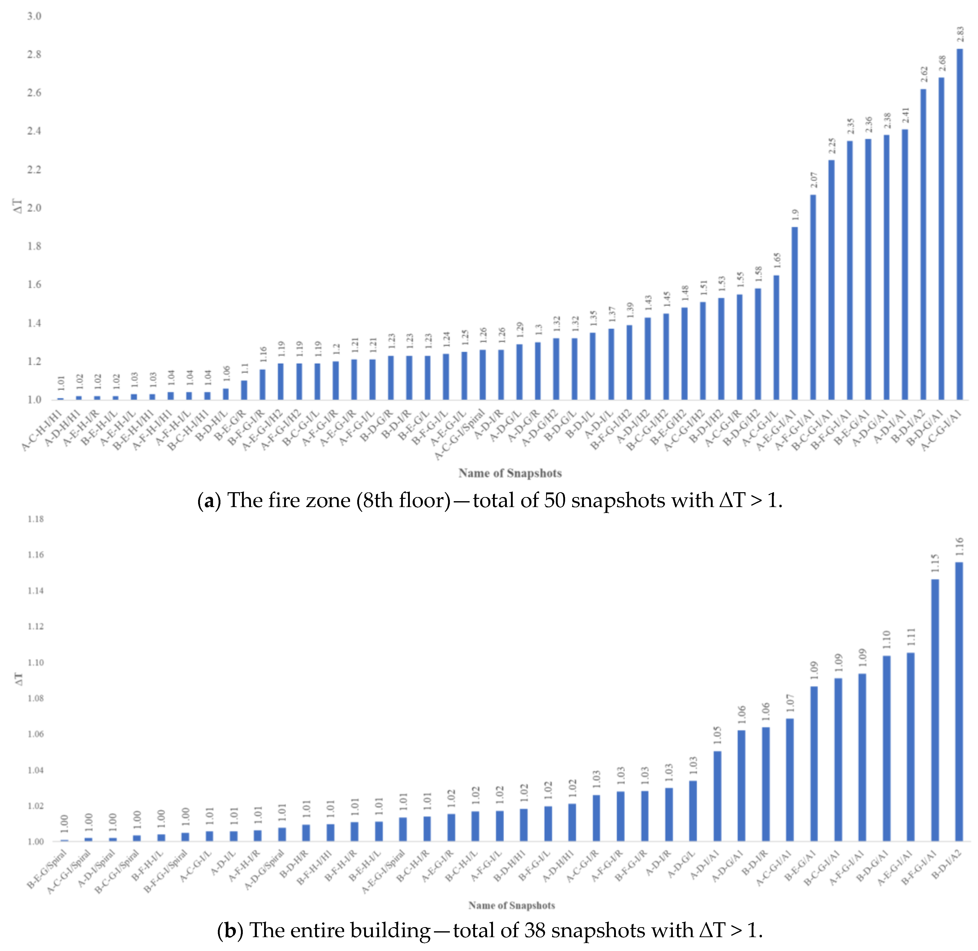
After running the fire and evacuation co-simulation, the evacuation time of the entire building and the 8th floor, as the scope of the investigation, were obtained for 90 snapshots with fire plus 18 snapshots without fire. Results showed that in eight snapshots with fire, the simulation did not converge, due to the blockage of the only available exit door (when the fire location is right in front of that exit and occupants are stuck). For a better illustration of the data associated with the 82 remaining with-fire cases, a ∆T parameter was defined as the ratio between evacuation times of each with-fire (RSET_{With Fire}) and without fire (RSET_{Without Fire}) scenario in the same snapshot. Based on this definition, ∆T can be in one of these three conditions: ∆T > 1, i.e., fires negatively impacting the evacuation time hence longer evacuation at the with-fire snapshots compared to without-fire ones; ∆T = 1, i.e., fire has no impact on the evacuation time; and ∆T < 1, i.e., the fire incident positively impacting the evacuation time, hence making the evacuation shorter. Figure 5 shows the distribution of the number of snapshots in each ∆T category in the entire building, as well as the 8th floor.

The ∆T > 1 category would be originally the expected case to approves the hypothesis of a longer time being required for the evacuation under the fire emergency. It is expected that, by implementing the fire, the agents’ visibility reduces and their speed would decline [30]. As a result, agents exposed to the smoke will have a slower evacuation and the whole evacuation time should be increased accordingly. Since the ‘without fire’ scenario’s evacuation time is considered as the safe baseline for each snapshot, the closer the evacuation times to the baseline (∆T to 1) the safer the scenario will be from the viewpoint of the fire evacuation. Therefore, ∆T can be considered as an indicator of the unsafe condition. The variation of ∆T values for both 8th floor and the whole building are illustrated in Figure 6.

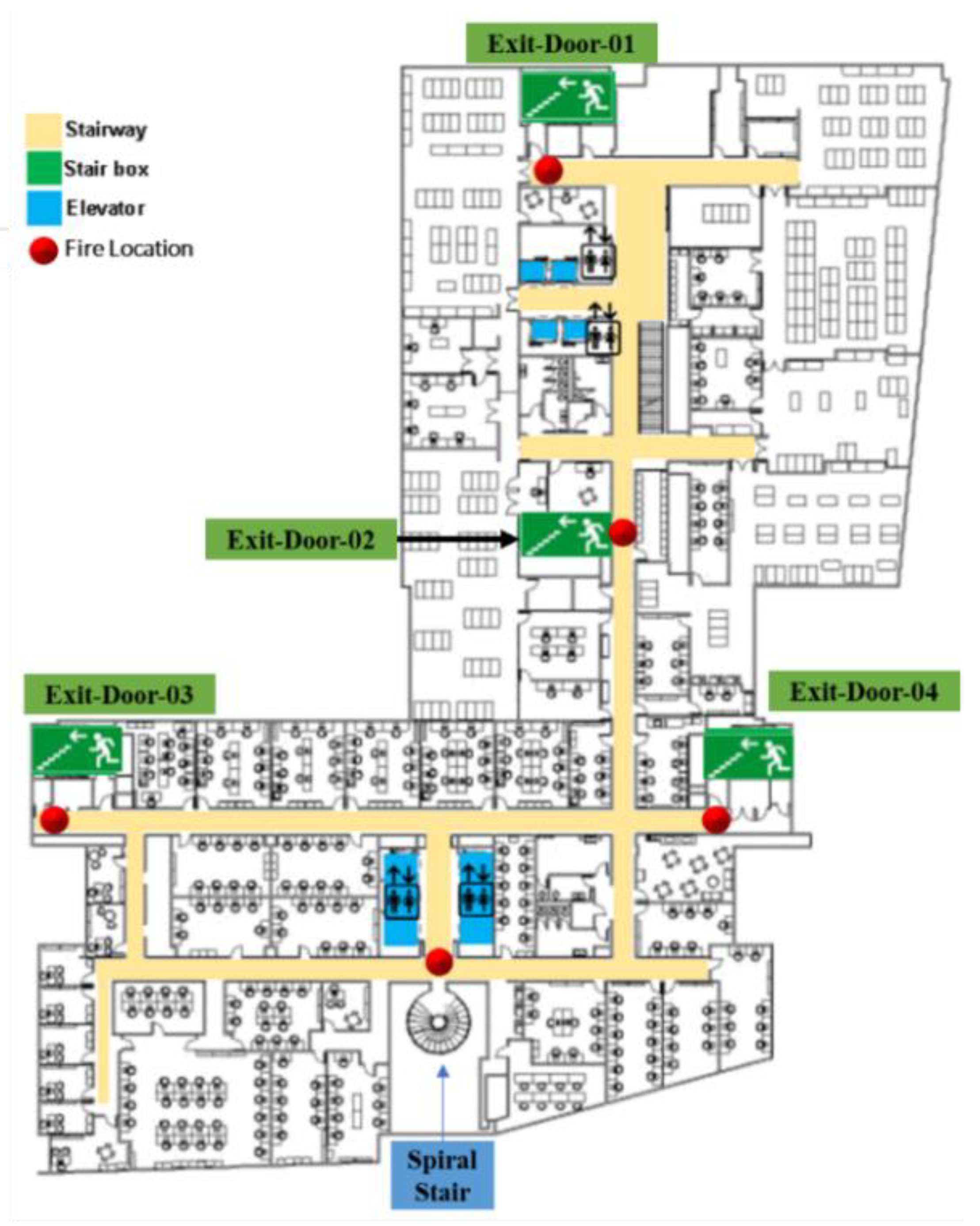
The two remaining categories, i.e., the same and faster evacuation time under the fire compared to the normal condition, appear contradictory to the hypothesis of longer evacuation in the presence of fire. Although the value of ∆T for most cases of ∆T < 1 is very close to 1.0 (between 0.87 and 0.998, with an average at 0.96 for the entire building and between 0.94 and 0.99, with an average of 0.98 for the 8th floor), and could have been attributed to the stochastic speed settings for the occupants; further investigations were made in the associated cases for both fire zone and the entire building, to identify the root cause. It was observed that three triggers control the evacuation time, which are critical egress, i.e., width of the door or staircase; the renovation operation location; and the fire location. For the cases where ∆T = 1 (i.e., the fire did not affect the evacuation time), it was concluded that the width of the door (Exit Door-2) and the staircase (Staircase-02) were the main influencers behind that. The exit door and staircase were narrower than the others, and thus occupants were more congested and evacuated more slowly through them. Accordingly, in these cases, the fire location was at the spiral stairs or the Exit Door-4 (please refer to Figure 3), the evacuation of these narrower locations was not impacted and thus the time was not changed. This phenomenon occurred in 22% and 8% of the cases related to the evacuation of the eighth floor and the entire building, respectively. To help support this analysis, Figure 7 shows the visibility range in different areas of the floor during the evacuation for different time steps, when the fire is in front of Exit Door-04 (Figure 7a) or the spiral Stair (Figure 7b). In all captured heatmaps, the red color means the horizontal visibility of 3.0 m, i.e., the full visibility range of an agent, and dark blue means the visibility of zero. In both figures, the area of congestion during the evacuation is marked. For all snapshots in the category of ∆T = 1, according to the fire slices results (Figure 7), propagation of smoke shows that in both mentioned fires, during the entire evacuation process, smoke does not reach the congestion area, hence will not impact the occupants’ speeds. All the evacuations are completed before 184 sec, which is when the visibility decreases in the congestion area. That is why the evacuation duration remains the same as in the case of not having any fire. Of course, the panic effect was not included in this study, and that can be considered one limitation of the simulation.

For the cases of ∆T < 1 (i.e., faster evacuation than without fire), the analysis showed different causes for the 8th floor and entire building. The agents are modeled to opt for the closest exit (shortest path). In the case of whole-building analysis, when narrower staircases are blocked due to construction or fire, the occupants select the other (wider) exits, which speeds up the overall evacuation. This indicated that the width of stairs was a more influential factor than the fire, when the fire was placed in the E-block of the building. In the case of 8th floor, by the time the occupants get into the congestion, there is yet no smoke there, because the source of fire is far from the critical exit door. Hence, the with and without fire evacuation scenarios are almost the same, with a minor difference in the number of people in the congestion (∆T in most of these cases is slightly less than 1). Another interesting observation was when the smoke completely reaches the congestion, at t = 57 sec as shown in Figure 8. Checking the frame-by-frame evacuation behavior, in this case, suggests that the speed reduction due to the smoke has helped the congestion by moving the crowd more smoothly and letting the occupants (accumulated from the 8th floor and floors above) evacuate in less density and a shorter time. However, this behavior of the agent-based model may not be realistic and requires further investigation to be validated and justified. It is evident for the fire and evacuation community that due to the lack of collected behavioral datasets, the validation process which should be a primary step in evacuation modeling becomes very challenging. There is a general absence of uniformity for evaluating evacuation models, which is mostly subjective depending on the users’ acceptance. However, the International Standards Organization (ISO) published initially the ISO 20414:2020 standard named “Verification and validation protocol for building fire evacuation models” through the committee of FSE (ISO/TC 92/SC 4) which should help in the future with this issue [48,49].

5.2. Construction Planning Results (Time, Cost and Safety)

Three criteria were considered for the schedule evaluation, i.e., cost; time; and safety, each of which has a separate measure and evaluation process. While several different metrics can be used to measure each criterion, and also there would be various ways to combine the metrics, the multicriteria decision-making aspect is not within the scope of this paper, and future studies will be needed in this regard. Nevertheless, we test some possibilities, mainly to show how the proposed method of this paper can be used in quantitative decision analysis.

Table 7. Schedule categories based on duration and cost.

Schedule Type	Schedule Number	Crew Combination	Total Duration (Days)	Mode cost ($)
1	Schedule 1 to 16	1 crew (lab)–1 crew (corridor)	65	60
2	Schedule 17 to 24	2 crew (lab)–1 crew (corridor)	36	120
3	Schedule 25 to 32	2 crew (lab)–2 crew (corridor)	36	160

compares the three schedule types in terms of the metrics used for cost and time. Starting with the time criterion, the final 32 schedules had a total project duration of 65 days for schedule type 1 (1 crew–1 crew) and 36 days for both type 2 and 3 alternatives (i.e., 2 crews–1 crew and 2 crews–2 crews). Given the high demand for access to the labs, it was assumed, as an owner requirement, that the desired project duration is 60 days or less. Moving on to the cost metric, considering that the only cost component modeled in the project is the direct cost (leading to the independence of project budget from duration), the authors used the ‘mode cost’, i.e., cash flow analysis, as a metric for cost evaluation. The mode cost was considered as the ‘highest most frequent daily cost’ throughout a schedule. Schedule type 1 with $60, schedule type 3 with $120, and schedule type 2 with $160, had the lowest to highest mode costs, respectively. Following the regular logic of construction projects, it was assumed that any contractor would prefer the lowest mode cost. Accordingly, the assumed metric for the cost was having a mode value less than $160.

For the third criterion, i.e., safety, two parameters were considered: fatalities and evacuation time. The occupants’ lives were considered paramount; therefore any schedule that had a snapshot with fatality was eliminated. Twelve schedules consisted of eight snapshots with fatalities, all of which were considered unacceptable. On the other hand, for the evacuation times (the remaining 82 snapshots), those with ∆T < 1 were assumed to be safe (until further studies will make better clarifications regarding the anomalies explained earlier). After that, two different methods were applied to provide a metric for the safety of each schedule.

Method A, Average total evacuation extension—In the first method, five ∆Ts per snapshot (one ∆T for every fire incident modeled), as expressed by Equation (1), are averaged to obtain the total evacuation time extension due to the fire, as $\Delta T_{tot}$ in Equation (2).

$$\Delta T_{Snapshot}=\frac{RSE{T}_{With-Fire}}{RSE{T}_{Without-Fire}}$$

(1)

where $RSE{T}_{With-Fire}$ is the required egress time in fire scenario and $RSE{T}_{Without-Fire}$ is required egress time in the baseline scenario (without fire).

$$\Delta T_{tot}=\frac{{\sum }_{i=1}^5\Delta T_{Snapshot}}{5}$$

(2)

where $\Delta T_{Snapshot}$ is calculated from Equation (1) and i is associated with the fire scenarios (from 1 to 5 in our case study with considering five different fire incidents). The $\Delta T_{tot}$ for each snapshot is then multiplied by the duration of that snapshot to calculate the fire risk of the snapshot ($F{R}_{Snapshot}$) as shown by Equation (3).

$$F{R}_{Snapshot}=\Delta T_{tot}\times Duratio{n}_{Snapshot}$$

(3)

where $\Delta T_{tot}$ is the summation of all $\Delta T_{Snapshot}$ related to one specific snapshot with five different fire scenarios and $Duratio{n}_{Snapshot}$ is the time of each snapshot occurrence in the schedule. It must be noticed that we are assuming similar likelihoods for the incident of all five different fires.

In each schedule, all values of $F{R}_{Snapshot}$ are summed up, and the $F{R}_{schedule}$ is eventually calculated as the factor of safety for the alternative schedule, as shown by Equation (4).

$$F{R}_{schedule}={\displaystyle \sum }_{i=1}^{n}F{R}_{Snapshot}$$

(4)

where $F{R}_{Snapshot}$ is derived from Equation (3) and i is the number of different snapshots existing/ considered in one schedule.

Method B, Maximum evacuation extension—In the second method, the maximum of five different ∆Ts is selected as $\Delta T_{max}$, as suggested by Equation (5). In each schedule, the maximum $\Delta T_{max}$ for different snapshots of the schedule is considered as the safety factor ($F{R}^{\prime }$) as shown by Equation (6).

$$\Delta T_{max}=Max(\Delta T_{Snapshot}{}_i)$$

(5)

where $\Delta T_{Snapshot}$ is the difference between evacuation time in with and without fire scenarios and i is associated with the fire scenario (from 1 to 5 for our case study).

$$F{R^{\prime }}_{Schedule}=Max( \Delta T_{max}{}_i)$$

(6)

where $\Delta T_{max}$ comes from Equation (5) and i is associated with the fire scenarios (from 1 to 5 in our case study).

Both methods A and B were applied to both fire zone and the entire building evacuation times separately, for our case study. The results were combined with the other two criteria, i.e., time and cost, to compare the construction schedule alternatives, as will be explained in the next section.

5.3. Construction Planning Evaluation

It is worth noting again that developing a multi-criteria schedule evaluation has been beyond the scope of this paper. The main objective of this study was to introduce co-simulation as a tool for quantitative analysis of safety in construction renovation projects. However, to show how the result can be mixed with other traditionally used metrics to evaluate schedules, i.e., time and cost, one simple combination option, i.e., weighted summation, is tested here. Further studies are necessary to determine the optimal weights, as well as better options for the metrics and multi-criteria function.

After calculating the three performance metrics for the assessment of the schedule, we define ‘TCS’ as an index to evaluate the goodness of construction scenarios. TCS in this study was defined as the weighted sum of the range-normalized values for these three metrics, for each alternative schedule, as shown by Equation (7). The aim is to identify the schedule with the lowest TCS. We used both versions of FR and FR’ and calculated the TCS twice for the case study. Detailed results are shown in Appendix A.

Table 8. TCS values for the Eighth floor based on method A.

Schedule	Snapshot Duration	∆T Tot	FR Snapshot	Raw Values			Range Normalization			TCS	Fatality?	Rank
				FR Schedule (Safety)	Cost	Time	Safety	Cost	Time
16	1	1.00	1.000	1	60	65	0.000	0.000	1.000	0.300	No	1
17	1	1.00	1.004	10	160	36	0.629	1.000	0.000	0.489	Yes
	2	1.49	2.985
	4	1.54	6.175
18	4	1.54	6.175	6	160	36	0.355	1.000	0.000	0.406	No	4
19	1	1.02	1.016	10	160	36	0.626	1.000	0.000	0.488	Yes
	3	1.54	4.631
	3	1.49	4.478
20	4	1.49	5.970	6	160	36	0.341	1.000	0.000	0.402	No	3
21	3	1.00	3.012	14	160	36	0.885	1.000	0.000	0.565	Yes
	2	1.02	2.032
	2	1.56	3.121
	4	1.43	5.734
22	2	1.43	2.867	9	160	36	0.556	1.000	0.000	0.467	No	5
	4	1.56	6.241
23	4	1.02	4.065	8	160	36	0.479	1.000	0.000	0.444	Yes
	1	1.00	1.004
	2	1.46	2.917
24	4	1.46	5.834	6	160	36	0.332	1.000	0.000	0.399	No	2
25	6	1.76	10.565	16	120	36	1.000	0.600	0.000	0.480	Yes
	4	1.00	4.011
	1	1.00	1.004
26	6	1.33	8.007	12	120	36	0.759	0.600	0.000	0.408	Yes
	2	1.02	2.039
	2	1.01	2.022
27	6	1.38	8.274	13	120	36	0.846	0.600	0.000	0.434	Yes
	4	1.01	4.038
	1	1.02	1.016
28	6	1.43	8.582	13	120	36	0.796	0.600	0.000	0.419	Yes
	2	1.00	2.000
	2	1.01	2.028
29	6	1.00	6.016	15	120	36	0.927	0.600	0.000	0.458	Yes
	4	1.76	7.043
	1	1.46	1.458
30	6	1.02	6.117	11	120	36	0.713	0.600	0.000	0.394	Yes
	2	1.33	2.669
	2	1.31	2.617
31	6	1.01	6.056	13	120	36	0.832	0.600	0.000	0.430	Yes
	4	1.38	5.516
	1	1.56	1.560
32	6	1.00	6.000	12	120	36	0.736	0.600	0.000	0.401	Yes
	2	1.43	2.861
	2	1.43	2.867

shows the results of Method (A) for the eighth floor.

$$TCS=w_{1}Time+w_{2}Cost+w_{3}Safety$$

(7)

where $Time$ is the normalized total duration of the schedule completion, $Cost$ is the normalized most repetitive daily cost (mode cost) in the associated schedule, $Safety$ is the normalized safety metric explained earlier, and the weights w₁ through w₃ are user-defined (for the sake of this paper, we applied equal weights to each metric).

As shown in

Table 9. Schedule Preferences based on evaluation methods.

Evaluation Method	Min TCS	Max TCS	Average TCS	Preferred Schedule	TCS Value
Method A—8th Floor	0.3	0.565	0.434	24	0.399
Method A—Whole Building	0.3	0.6	0.453	20	0.391
Method B—8th Floor	0.3	0.565	0.434	24	0.399
Method B—Whole Building	0.3	0.482	0.461	20	0.476

, any schedule that had a snapshot with fatality was eliminated from the selection process, leaving schedules 16, 18, 20, 22, and 24 to decide between. Logically, schedule 16 provided the lowest TCS for both the 8th floor fire zone and the whole building; however, it violated the core owner requirement of a duration less than 60 days and hence was also excluded from the comparison. Consequently, this table shows the TCS values for each evaluation method for the 17 schedules and the corresponding best schedule.

6. Conclusions

This study developed a framework to quantitatively investigate the effect of occupant’s fire and evacuation safety as an additional decision criterion on construction renovation schedules. To implement this investigation a building examination was conducted to provide the relevant properties related to the construction scope and evacuation (size, number of floors, number and location of exits, layout, etc.). All the possible construction scenario combinations were obtained and filtration techniques with regards to the construction flow and building operation logic were applied to select viable construction plans. Workspace modeling was applied to the acceptable construction scenarios to determine the unique building layouts under construction. Then fire scenarios and properties were generated for each snapshot of the renovation operation. By the aid of BIM and FDS applied over the BIM environment, fire effects were simulated and evacuation behavior of occupants was modeled through ABM. The results were analyzed and evaluated according to the defined metrics to measure the goodness of construction schedules under cost, time and safety criteria. By integration of Pyrosim and Pathfinder and running the co-simulation, two RSETs (required safe exit time) were obtained. The first RSET was based on the scenario with fire (for various scenarios) and the second RSET was the scenario without fire. The proportion of these two numbers provided an indicator of risk; the greater this number, the higher the fire risk of that snapshot. Two methods were applied on the basis of this indicator to assign a number related to safety to each schedule. To evaluate the schedules, the possibility of fatality and casualties were investigated and all the schedules consisting of such construction scenarios were eliminated. An indicator, called TCS, was introduced as the weighted summation of cost, duration, and risk factors. The risk factor was calculated for the fire zone where the fire initiates, as well as the entire building, in two different ways.

The main contribution of this study is to propose a methodology to integrate fire safety analysis quantitatively in the process of construction planning for renovation projects. The results of this analysis consist of 44 TCS values for the two tested methods of assessment with two different approaches of safety calculation. By analyzing the co-simulation results, it was verified that the presence of fire in renovation work increased the evacuation time in 60% of cases in the fire zone of fire origin, and about 40% of cases in the whole building. Moreover, it was apparent that the construction schedule with minimum cost or budget will not necessarily be the safest in all cases. The start point of the fire was considered correlated with the construction workspaces where combustible materials are compiled. It was shown that the fire origin can significantly influence the criticality and increase the safety risks of the scenarios. Among selected fire locations, the fire in front of the open spiral stair connecting the three floors of the fire zone had the least impact on evacuation, due to the chimney effect.

Despite the contributions, this study had some limitations and made assumptions that need further investigations in the future. The proposed method takes into consideration the higher risk associated with building blockages that take longer; however, the same likelihood was considered for the occurrence of all fire scenarios; which in the future should be scrutinized in more detail. The probability of fire in various workspaces, for instance, can be assumed to be proportional to the amount of fuel available in those spaces, and the propagations can be modeled accordingly. Furthermore, the impact of the fire on agents’ behavior was limited to view reduction due to smoke. However, fire flashover, other fire products’ impacts, the panic effects, and the behavior of occupants with physical limitations must be further investigated in the future. The effect of sprinkler and HVAC systems and the probability of any failures (in pressurized stairs, e.g.,) were ignored in the presented co-simulation, which can be another area for future research.

Last but not least, while the proposed methodology can help construction planners integrate safety in their construction modeling procedure, the decision making based on this additional criterion requires further research. As construction scheme analysis is not limited to cost, time, and safety, more comprehensive studies will be needed to select accurate metrics, assign proper weights, and combine the criteria appropriately so that the construction planners assure the selection of the most ideal construction schedule.