Self-AdaptIve LOcal Relief Enhancer (SAILORE): A New Filter to Improve Local Relief Model Performances According to Local Topography

Abstract

The use of Light Detection and Ranging (LiDAR) is becoming more and more common in different landscape exploration domains such as archaeology or geomorphology. In order to allow the detection of features of interest, visualization filters have to be applied to the raw Digital Elevation Model (DEM), to enhance small relief variations. Several filters have been proposed for this purpose, such as Sky View Factor, Slope, negative and positive Openness, or Local Relief Model (LRM). The efficiency of each of these methods is strongly dependent on the input parameters chosen in regard of the topography of the investigated area. The LRM has proved to be one of the most efficient, but it has to be parameterized in order to be adapted to the natural slopes characterizing the investigated area. Generally, this setting has a single value, chosen as the best compromise between optimal values for each relief configuration. As LiDAR is mainly used in wide areas, a large distribution of natural slopes is often encountered. The aim of this paper is to propose a Self AdaptIve LOcal Relief Enhancer (SAILORE) based on the Local Relief Model approach. The filtering effect is adapted to the local slope, allowing the detection at the same time of low-frequency relief variation on flat areas, as well as the identification of high-frequency relief variation in the presence of steep slopes. First, the interest of this self-adaptive approach is presented, and the principle of the method, compared to the classical LRM method, is described. This new tool is then applied to a LiDAR dataset characterized by various terrain configurations in order to test its performance and compare it with the classical LRM. The results of this test show that SAILORE significantly increases the detection capability while simplifying it.

1. Introduction

Airborne laser scanning (ALS) is a tool now widely used in archaeology [1,2,3,4,5,6,7,8], geomorphology, and earth sciences [9,10,11] to detect natural landforms or remains of human activity, especially in forested areas, where other remote sensing techniques are unsuccessful or time-consuming. The main interest of this technology is to cover large areas while offering high spatial resolution capabilities. Research programs using LiDAR data are becoming more and more frequent. These studies are very often based on a multidisciplinary approach, involving specialists in archaeology, forestry, geomorphology, volcanology, etc., [12]. After ALS data acquisition, a point cloud classification has to be carried out, and the resulting Digital Terrain Model (DTM) and Digital Surface Model (DSM) areas are produced. The DTM is the result of the classification of bare-earth elevations [13,14], removing the vegetation and/or buildings, while vegetation and buildings are included in the DSM. Different visualization techniques are then generally applied to the DTM, to enhance micro-topography versus global topography and help to the detection of target features. The most common are multidirectional oblique weighting hillshade (MDOW), slope [15], Local Relief Model (LRM) [16,17], Sky-View Factor (SVF) [18], positive and negative openness [19,20]. These methods can be divided into two main categories: hillshade, Sky-View Factor, and openness are typically illumination techniques, based, respectively, on the sky portion visible from each position or on the openness characteristics of the relief at each position. They allow highlighting high-frequency components of the relief but remove all the elevation information. Indeed, these methods do not directly restore the topographic variations but rather the consequences of these variations, such as the portion of the visible sky. On the contrary, slope and LRM are DEM manipulating methods. They consist in computing elevation characteristics parameters, respectively, the slope or the high-frequency component of the relief. This information can then be exploited and interpreted directly for archaeology or geomorphology. Recent studies proved that LRM is one of the most efficient visualization techniques [21,22]. The basic principle is to apply moving average filtering to the DTM, in order to remove the general trend of the natural relief: the local relief, characterized by sharp variations, is then revealed [16]. The extent of this filtering (kernel- or window-size) has to be defined by the user, according to both global relief characteristics and morphometric characteristics of the target features. The choice of the correct filtering extent is important but not critical when it is applied to the detection of well-preserved anthropogenic remains. This is because they are generally characterized by sharp changes in local relief, corresponding to the high-frequency component in the frequency domain, well separated from the lower frequency component (features of the natural relief). However, when the aim is to detect all the potentially interesting features, including geomorphological shapes or eroded anthropogenic remains, the filtering perimeter has to be adapted to the characteristics of the natural relief (e.g., slope), which influence the performance of the LRM significantly. Indeed, it is only possible to detect an artifact if it provides a sufficient contrast compared to the surrounding features, i.e., if its frequency signature is significantly higher than the one of the natural reliefs [23]. As LiDAR detection is now used on very large areas, several LRM configurations need typically to be used in order to detect both slight and sharp local relief variations in complex topography contexts, including flat areas and medium to steep slope areas, after what the results from the different models could be eventually merged. This process can be confusing and time-consuming, especially for inexperienced users, and also introduces significant bias, as the decision of the configurations to be tested depends on the skills (and the available time) of the operator. The aim of this paper is to present an evolution of this widely used Local Relief Model method, allowing the automatic adaptation of the filtering size according to natural relief, producing a single-model, which makes simpler, faster, more efficient, and more reliable detection of target features in large datasets with variegated topography. This Self-AdaptIve LOcal Relief Enhancer (SAILORE) automatically uses the best filter configuration, allowing the detection of all the types of anthropogenic remains, independently of the global relief context. In this paper, we first present in the material and method section the study site and the LiDAR dataset, containing various types of anthropogenic structures coupled with a high variability of natural reliefs. Then, we present the LRM principles, the SAILORE approach and the details of the algorithm. Finally, in the results section, we compare LRM and SAILORE filtering on two test windows, including various relief configurations (plains, slopes, plateaus) and several types of target features. In conclusion, the differences are explained and discussed, pointing to advantages, limits, and future developments of this new algorithm.

2. Materials and Methods

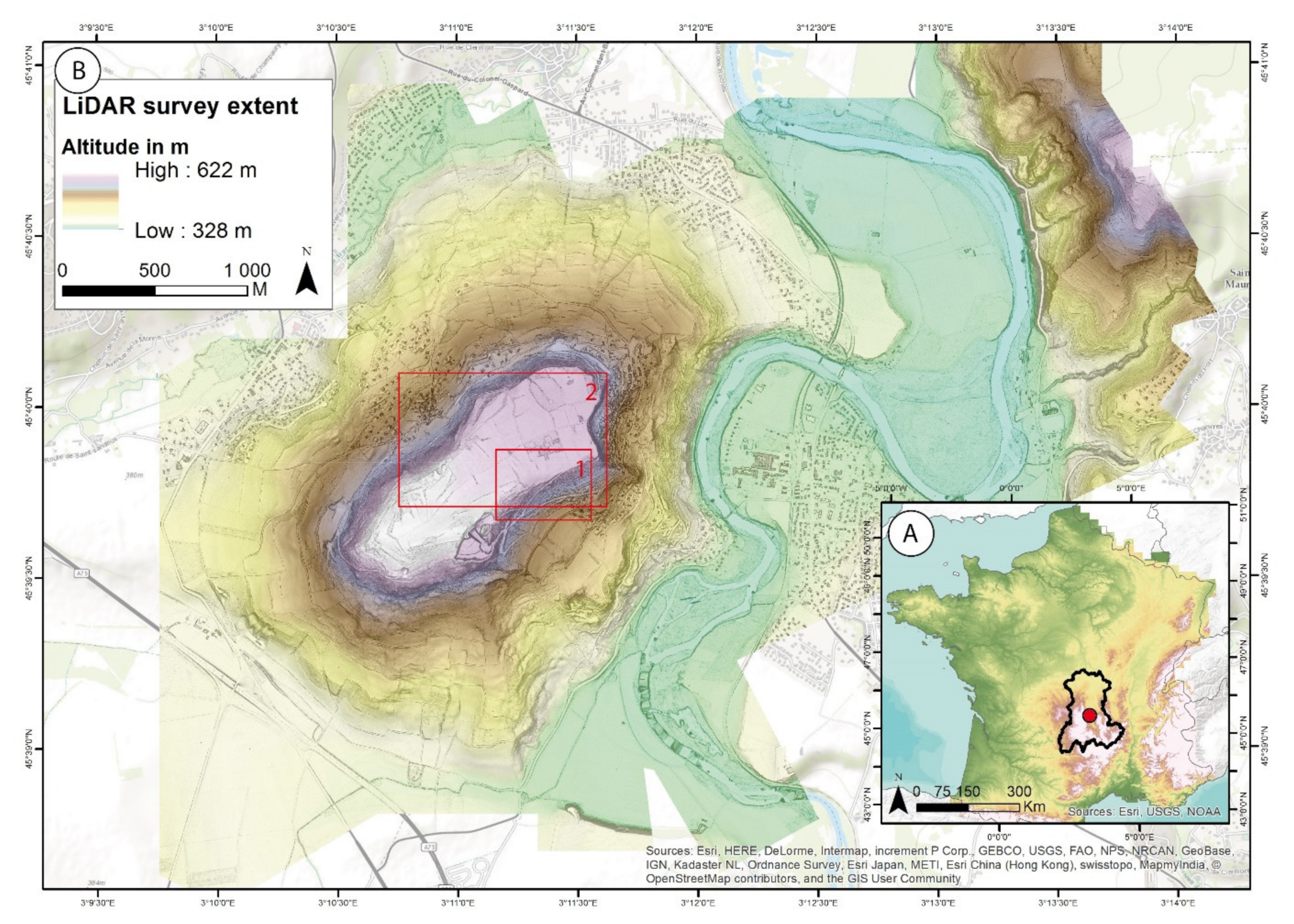
2.1. Airbone Laser Scanning Data and Derived Dataset

In order to test the performance of the proposed approach, a high-resolution LiDAR dataset covering a large zone with various relief configurations and with a high concentration of archaeological remains in various conservation status was used. Its acquisition was carried out as part of a multi-disciplinary program called AYPONA and focused around the basaltic plateau of Corent (Auvergne, France) [24]. It covers an area with heterogeneous relief, such as the floodplain of the Allier river, terraced slopes managed for vine growing, and quarries for basalt extraction [25]. The plateau summit is an exceptional archaeological site, with a continuum of human settlements from the Neolithic to the late Middle Ages periods [26,27]. A wide variety of anthropogenic landforms can then be detected throughout various relief configurations and with a more or less visible trace in the field. Figure 1 shows the location of the study area and the extent of the LiDAR survey.

LiDAR data were collected in March 2014, after the winter period when snow often recovers the ground and before the growth of the deciduous tree leaves. A high density of 18 laser pulses per square meter was emitted at a flight altitude of 500 m and covering an area of 22 km² with 19 flying lines in 2 perpendicular directions. This acquisition was carried out with a Litemapper 7800 [28]. The aircraft, a Piper PA-23 Aztec, collected the data at a speed of 100 km/h. Several control points were acquired on the ground to improve the accuracy of the positioning. The scan data adjustment protocol was processed with RiProcess v1.5.8 software.

The LiDAR point-cloud classification was performed using the Multiscale Curvature Classification for LiDAR Data (MCC-LiDAR) algorithm [29]. Bare earth returns were interpolated using the natural neighbor method and converted into a regularized raster DTM, with a 0.50 m grid in the x-y plane and with height values expressed in meters. A 0.50 m pixel size was chosen as the best compromise between a precision sufficient to preserve most of the detail of bare earth point clouds, allowing the detection of anthropological features and reasonable size of the raster DEM file (588 Mb, for a 13,811 × 10,770 matrix in our case). The windows used to carry the tests and the comparisons (see below) are characterized by varied landforms concentrated on quite small areas. Moreover, all these types of landforms configurations have been impacted by human activities, even in the case of steepest slope sectors, which have been terraced.

2.2. Principle of the Local Relief Model and of the SAILORE Method

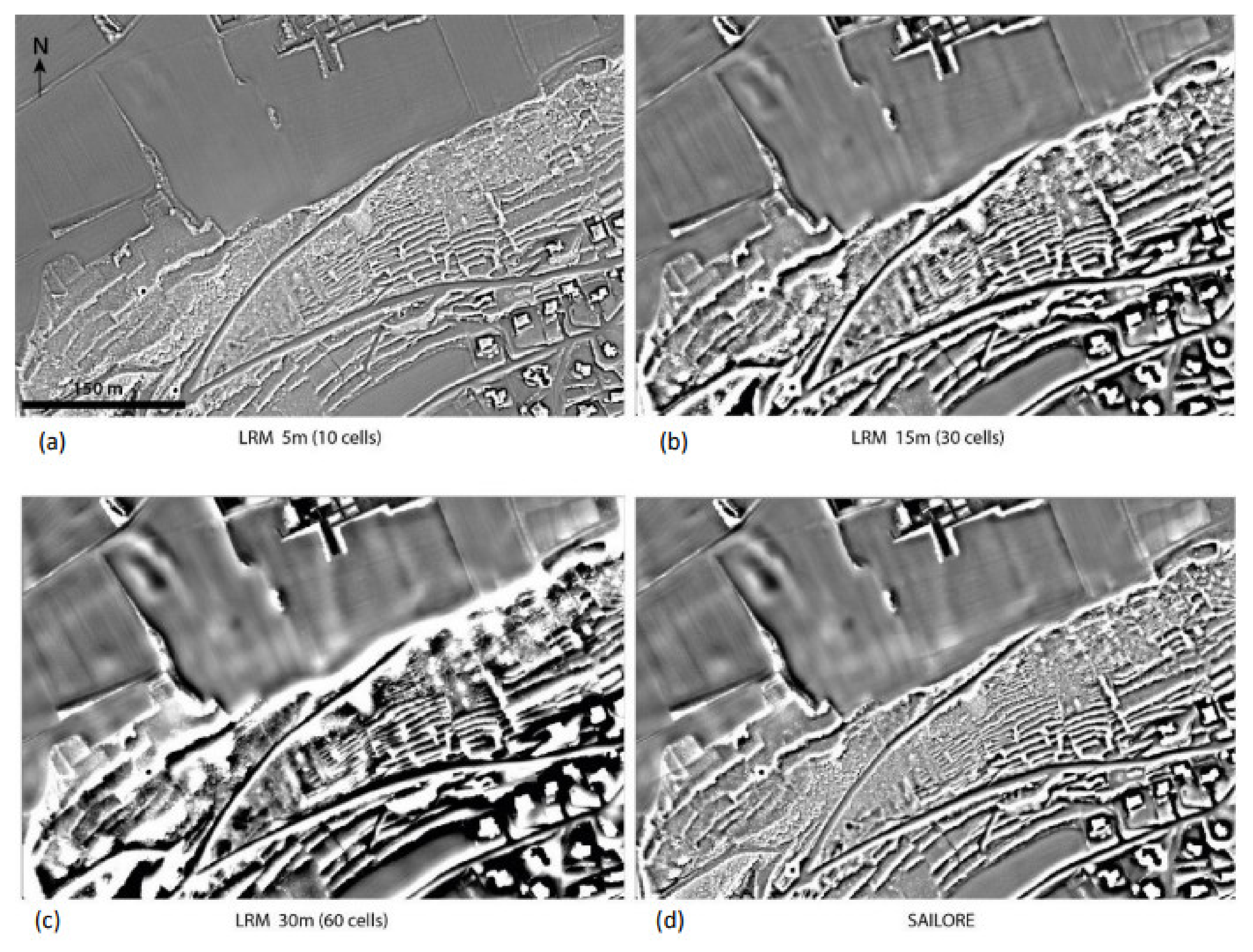
2.2.1. The LRM Principles

The SAILORE method is based on the principle of the Local Relief Model algorithm [16], summarized hereafter. The first step consists in the application of a low pass filter to the DEM generated by the classification of the initial LiDAR point-cloud. This low pass filtering aims to smooth the DEM, in order to approximate the general relief trends and the large-scale landforms. The neighborhood (or kernel) size of the low pass filter was crucial to determine the scale of features that will be visible in the LRM. The result of this low pass filtering was then subtracted from the DEM to obtain the local relief: the obtained result actually consists in applying a high pass filter to the DEM. At this step, the zero contour lines were extracted from the map resulting of the high pass filtering and the DEM’s elevation values were extracted along these contour lines. A new large-scale artificial smoothed DEM was then generated from the interpolation of these values and was finally subtracted to the original DEM to create the Local Relief Model.

In the LRM approach, the neighborhood (or size) of the low pass filter was unique in each run of the algorithm and has to be set each time by the users. Generally, it is the result of a compromise: if the chosen kernel is too small, the filtering effect decreases, and the slightest terrain variations (low-frequency components) will not be detectable (Figure 2). On the contrary, if the chosen kernel is too large, the filtering effect will increase and the higher frequencies of the natural relief will not be removed. In this last case, all the information about the target features will be present in the LRM, but their readability will be worsened because they will be intertwined with non-interesting features that should have been filtered. However, once the user has fixed a kernel size, the configuration of the terrain (mainly slope) is still one major factor affecting the results of the LRM [23], and different settings will be needed to detect and delineate properly similar objects in flat, hilly, or steep slope areas.

2.2.2. The SAILORE Approach

In the SAILORE approach, the filtering effect was adapted to the natural slope of the terrain, allowing the simultaneous detection of very small micro-relief variations on flat areas, as well as the identification of sharper relief variations in high slope sectors. The difference with the LRM lies in step 2 of the processing (see above): instead of applying the same low pass filtering to the whole DEM, an adapted low pass filter was computed for each pixel in order to take into account the global relief configuration. The interest of this method was to compute the optimal neighborhood size of the low pass filter for each specific terrain configuration.

If we consider the case of the land configuration represented in Figure 2a (a plateau area linked to a flat area by a steep slope), it can be divided into 2 components: the “natural” component (Figure 2b) and the anthropic component (Figure 2c). In our case, the natural component was characterized by low slope values on the plateau and in the valley and high slope areas at their interface. From a data processing point of view, the flat areas correspond to low frequencies and the slope areas to medium frequencies. To be detectable, artifacts of anthropogenic or geomorphic origin must be characterized by variations in altitude that were steeper than the surrounding environment, even if these variations were of small amplitude: they must, therefore, be characterized by frequency components higher than those of the natural component. This was the core principle implemented in the approach developed by Hesse for the LRM: remove the low-frequency component to keep only the high-frequency variations [14].

However, the main difficulty in that approach was that the boundary between low and high frequencies was difficult to determine because medium frequency signatures can be found in natural landforms as well as in traces of past human activities. In fact, even if the signature of human activity was almost systematically expressed by landforms with high (even vertical) slopes, these traces have very often been reshaped and strongly flattened by cultivation during several centuries on lowland areas. Conversely, as shown in Figure 2, the steepest areas of the natural relief (2b) can have steep variations without necessarily being of anthropogenic origin (e.g., slope screes or escarpments). In other words, the natural relief (2b) can be represented as the sum of very gentle variations (low frequency) on the flat areas (2d) and steeper variations (medium-frequency) on the slopes (2e). Similarly, the traces of human activities can appear as very steep variations (high frequency) in the slope areas but also softer variations (medium-frequency) on the flat areas. Mid-frequency components can represent both the natural relief in the sloping areas and the traces of human activities in the less sloping areas.

Figure 3 illustrates the potential problems that may arise in choosing the best kernel size for the LRM computation: if the chosen filtering radius is too large, some part of the natural relief may be still present in the LRM output, resulting in possible misinterpretation of the artifact (Figure 3(3)). On the contrary, on very flat areas, a filtering perimeter that is too small may cause eroded anthropic traces to disappear (Figure 3(2)). A consequence is that a fixed filtering size will be only optimal for a very restricted range of terrain configurations and suboptimal or even totally inadequate in most other areas. This leads the users to produce several LRMs in order to properly cover more terrain types, however in practical terms, the number of models, which can be produced, processed, and interpreted is reduced, and the coverage of optimal-LRM areas always remains limited. The solution proposed with the SAILORE processing was to take into account the nature of the landscape on a large scale in order to automatically adapt the filtering perimeter to the terrain configuration, without requiring any user intervention (Figure 3(1)): only potentially anthropogenic components are highlighted, whatever the relief is.

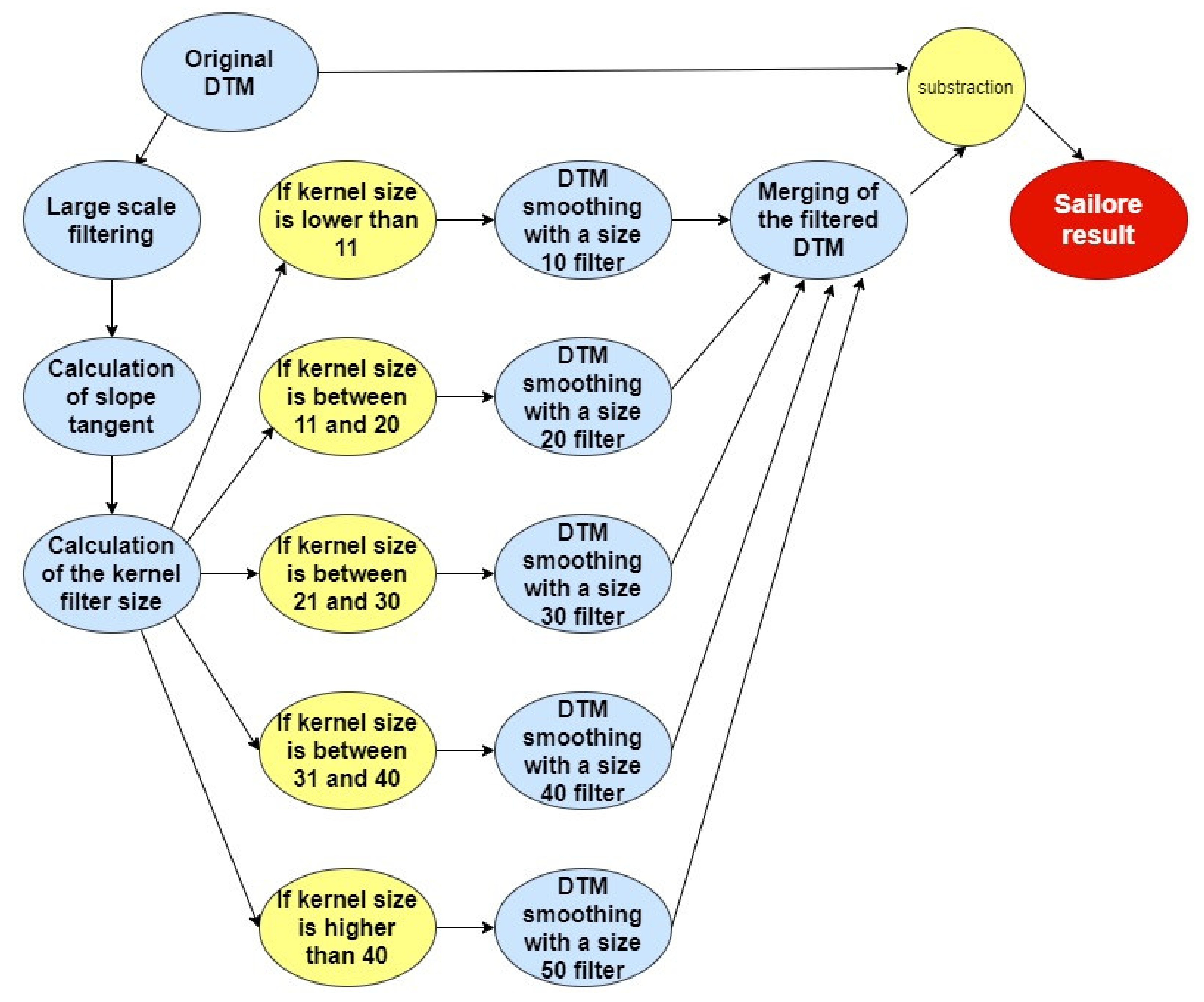
2.3. Description of the SAILORE Algorithm

Figure 4 summarizes the algorithmic approach implemented for the Self AdaptIve LOcal Relief Enhancer (SAILORE) processing in ArcGis^® environment (Model Builder).

The global process can be divided into several major phases:

(a)

Realization of a sliding average smoothing with a very large filter buffer (100 cells, or 50 m in our case, the DTM resolution being 0.5 m).

This low pass filter replaces each matrix element by the average value of the surrounding elements:

$$x_{n,m}=\frac{1}{N.M}{{\displaystyle \sum }}_{k1=n-\frac{N}{2}}^{n+\frac{N}{2}}{{\displaystyle \sum }}_{k2=m-\frac{M}{2}}^{m+\frac{M}{2}}{x}_{k1,k2}$$

(1)

where M represents the number of lines and N the number of columns of the filter applied to the data matrix. In our case, and for all the continuation, we will choose to take M = N for reasons of symmetry of filtering, and in the case of filtering evoked previously M = N = 100.

This first step allows to remove all the roughness of the DTM and to keep only the low-frequency component of the relief.

(b)

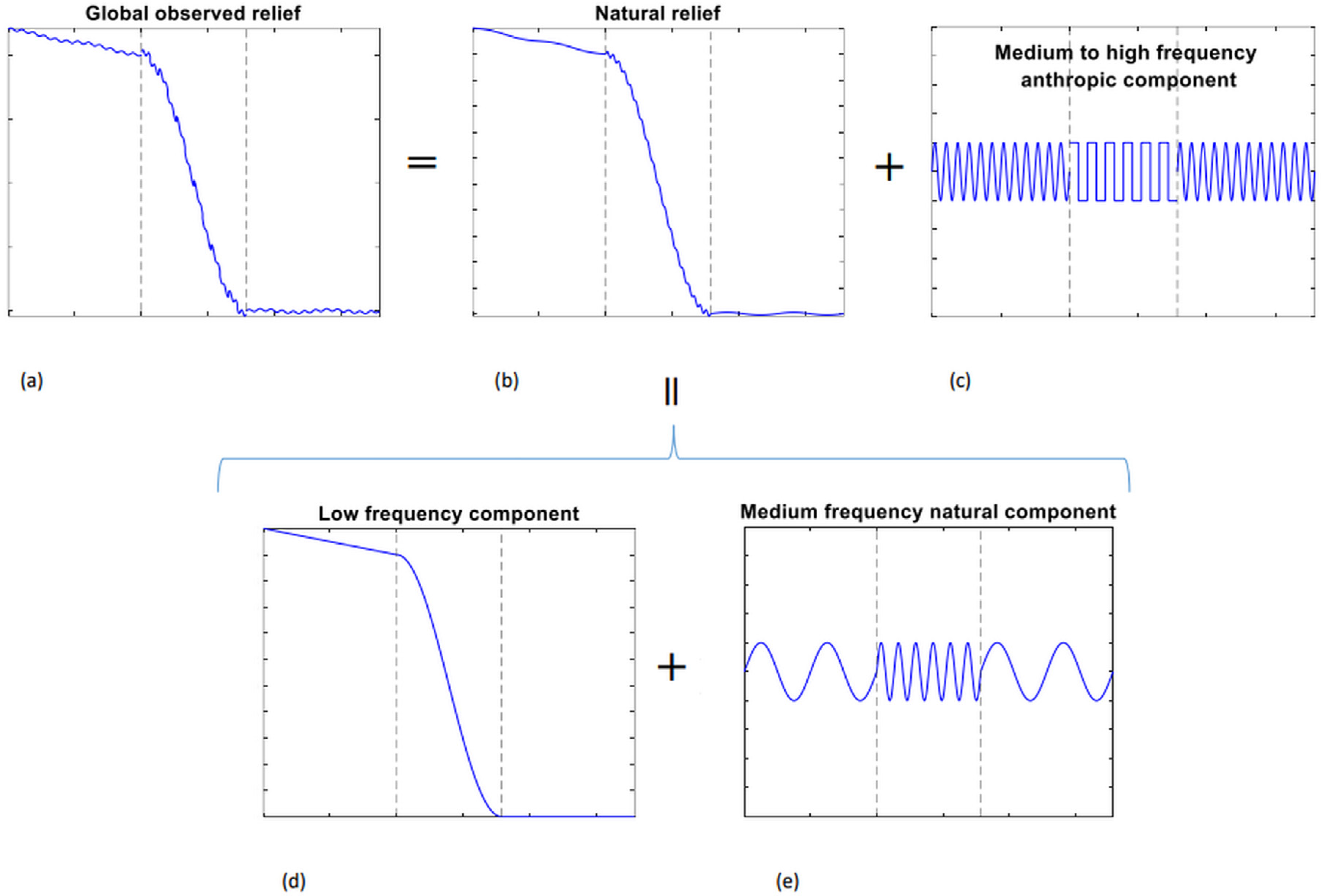
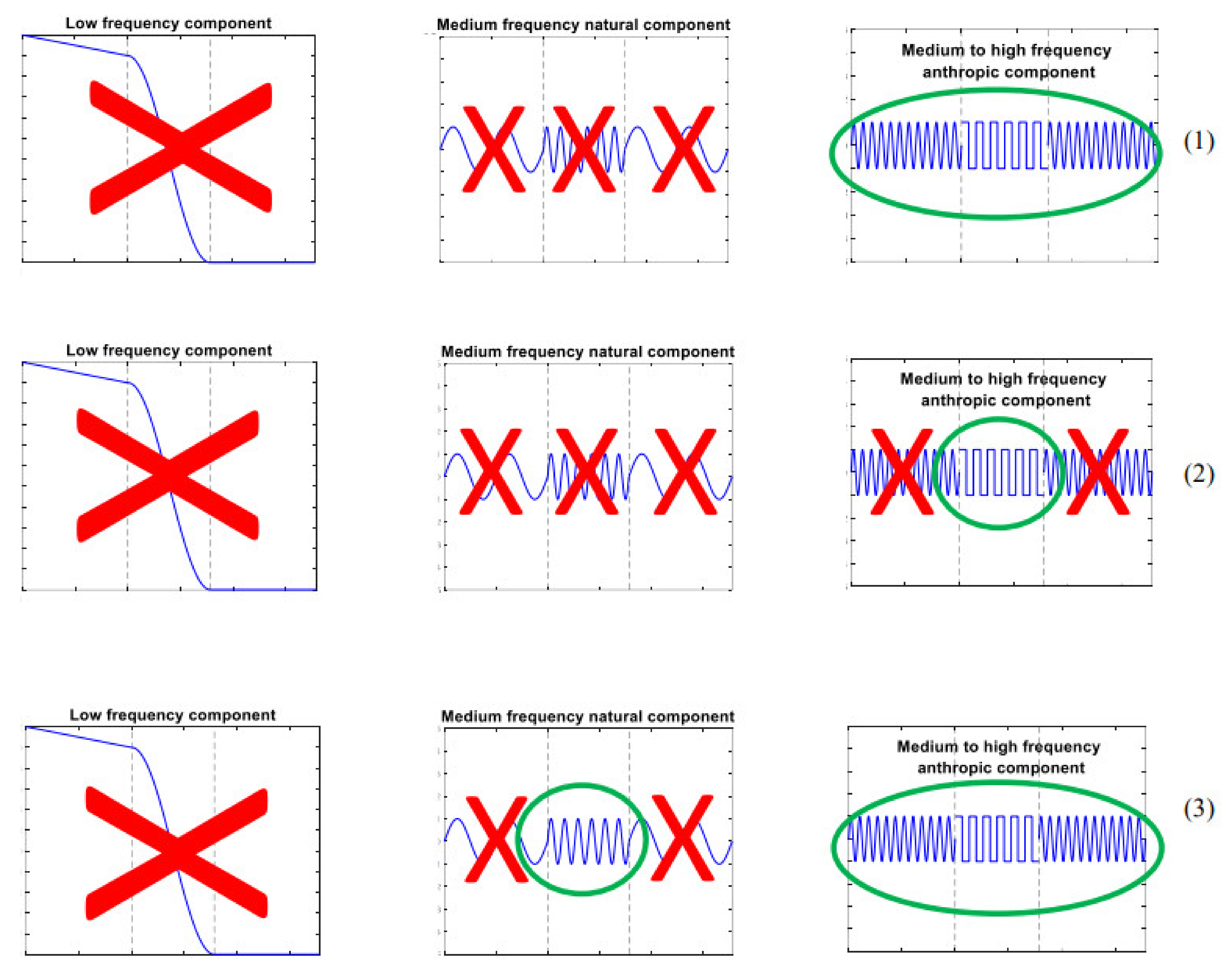
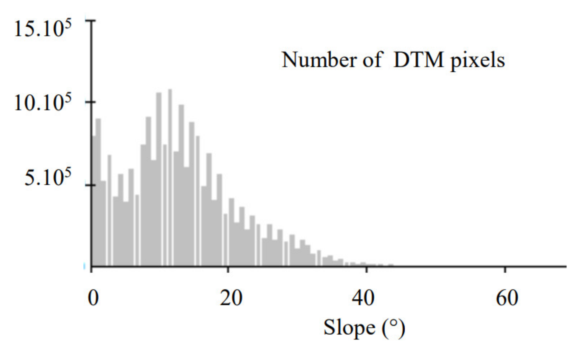
Calculation of the slope of this global relief, from which will be determined the size of the filtering buffer applied to each zone. The slope is calculated with the default procedure proposed in ArcGis^®, with a neighborhood of 3 × 3 cells. It was calculated from the previously smoothed DTM, and thus gives us information on the steepest slope around each pixel, expressed in degrees. This local slope value must be related to the size of the filtering kernel. The simplest way to proceed would be to adapt the size of the filtering area proportionally to the slope. If we look at the slope distribution from a statistical perspective (Figure 5), we can see that it logically follows a Weibull distribution, with a high occurrence of low slopes and very few values beyond 45°.

It appears that a linear relationship between the size of the filtering kernel and the value of the slope over the entire range 0–90° is not the most appropriate because it would deprive us of accuracy in the area of low slope, which constitutes the bulk of our data.

To solve this problem, we chose to work with the slope tangent because it is a non-linear function that relates the angle of the slope α, to the altitude variation dZ in the vertical plane and to the variation dX in the horizontal plane: tan(α) = dZ/dX.

In our case, dX is of special interest because it is the image of the size of the kernel that we wish to determine. By computing the kernel no longer proportional to the slope but inversely proportional to the tangent of the slope, we broaden the distribution of values of this kernel, thus increasing the resolution of the model (Figure 6).

In this case, the higher the slope, the higher the tangent of the angle, and, therefore, the smaller the inverse of the tangent, leading to a reduction of the kernel size. However, what is crucial here is the non-linearity of the tangent function, which grows slowly for small values and then tends to infinity when the angle tends to 90°. This means that the adaptation of the kernel size to the slope conditions will also be non-linear: for low slope areas (plateau and valley) the adaptation of the filter size will be limited, the kernel size remaining high, while in high slope areas, the adaptation of the filter size will be much finer, allowing a better adaptation to the relief variations.

(c)

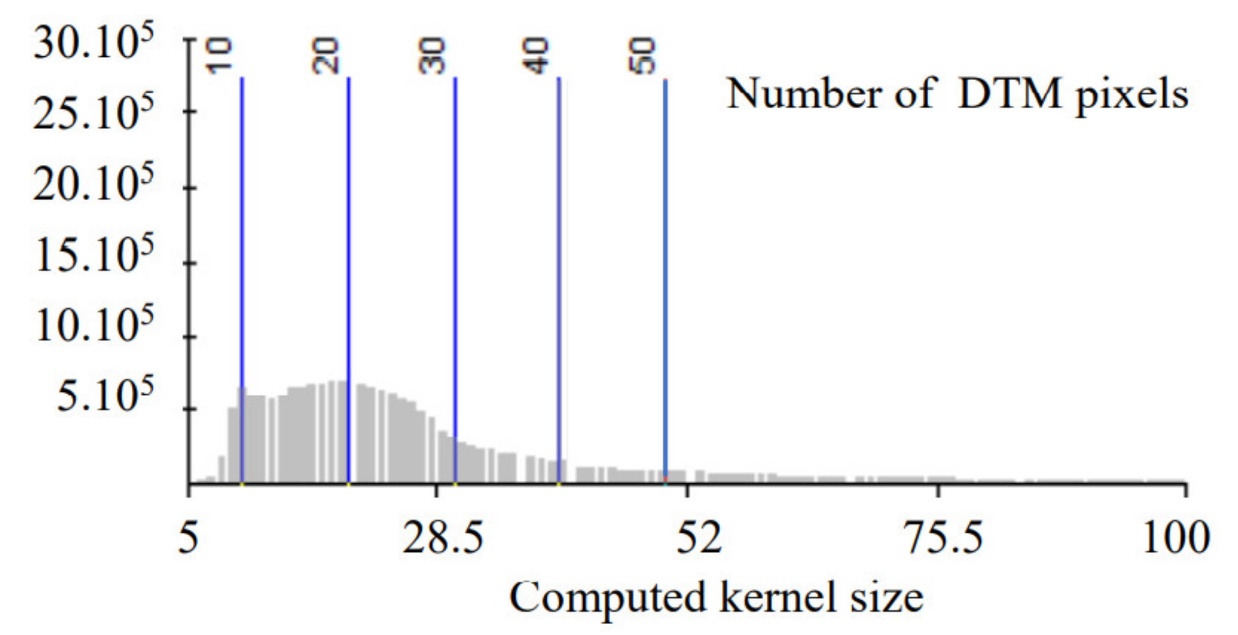
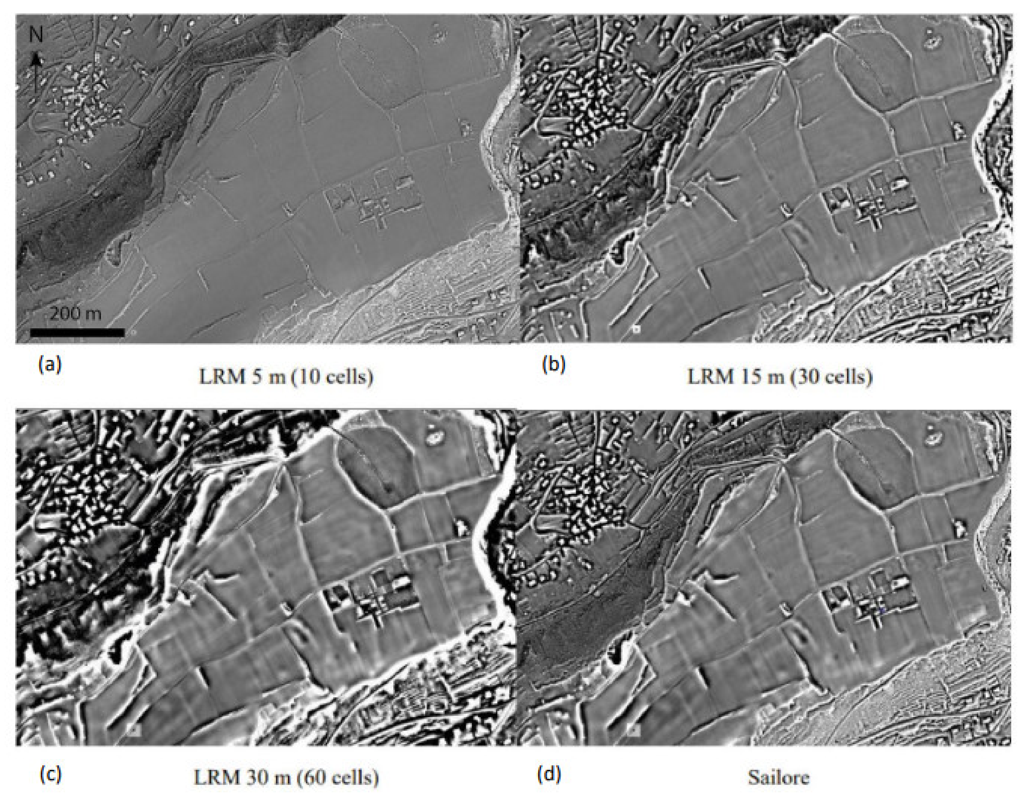
Differential smoothing of the original DTM. For this phase, in order to reduce the complexity of the model, 5 thresholds were chosen (see Figure 4 and Figure 6). The maximum kernel size was set at 50 pixels (25 m), which corresponds to half of the kernel chosen in the first phase to restore the global relief of the site by removing all medium and high-frequency components. Values of 60 and 80 pixels, respectively, were tested, and they led to very similar results, which is logical because this kernel size will be used on very flat areas, for which the quality of the filtering was not very sensitive to the size of the kernel, the pixels having all a similar value. The interest of the 50-pixel kernel was then to be less demanding in terms of computing time. The minimum kernel size was set to 10 pixels (5m), which also corresponds to the values classically used to highlight micro-variations of the relief. Indeed, from a practical point of view, a sliding average filtering does not make sense if it is performed at the scale of a few pixels, knowing that for a structure to be identified, even by an expert eye, it must include several 10s of pixels. Finally, 3 intermediate filtering levels, corresponding, respectively, to 20, 30, and 40 pixels, were defined (10, 15, and 20 m, respectively). These values were chosen to allow for a gradual transition between minimum and maximum kernel sizes and to accommodate areas of intermediate slopes. In the absolute, we could consider 40 successive levels, allowing to go from the filtering on 10 pixels to the filtering on 50 pixels with a step of 1, but this configuration, which complicates the model, does not bring a significant gain in terms of resolution, as we could notice it in our tests. The step of 10 pixels was thus chosen as the best compromise between the resolution obtained and the necessary computing time. It is important to note that the choice of these thresholds was independent of the calculation principle of our Self-AdaptIve LOcal Relief Enhancer and that they can be adapted if particular study contexts require it.

(d)

Finally, each pixel is associated with the filtering result of the threshold to which it corresponds, and the global filtered DTM is thus generated, pixel by pixel and then subtracted from the initial DTM, to provide the final visualization (Figure 4).

2.4. Testing the Performance of the SAILORE Approach

In order to compare the performance of SAILORE approach vs. conventional LRM, we applied both filtering algorithms to the available LiDAR dataset (see Section 2.1). For the LRM, we used 3 different settings for the filtering window size (5, 15, and 30 m), corresponding to the optimal configurations for high, medium, and low slopes, respectively. Then, we selected 2 comparison windows, including several typical terrain types: flat areas under cultivation with a few agricultural structures and archaeological remains, terraced steep slopes, and intermediate slopes with buildings (see Figure 7, Figure 8 and Figure 9). Finally, we carried out a visual comparison of the ability of all the processed images to detect the same features in both windows.

3. Results

The results of applying the LRM with the different settings and SAILORE algorithm to the DEM are shown in Figure 8 and Figure 9. In the case of window nº1 (Figure 8), each one of the LRMs shows different levels of performance depending on the terrain. The LRM with filtering of 5 m (10 cells) shows an image very close to a slope map. In the steepest slopes (center of the image), all the terraces are well delineated with sharp borders independently of their state of preservation. In the intermediate slope area (lower right corner) the result is also quite good. However, in the more or less flat areas of the summit of the plateau (center and upper-left corner), these settings of the LRM only detect the current agricultural walls and the trenches of the archaeological excavation.

The LRM with a filtering radius of 15 m shows much better results in the cultivated flat areas of the plateau: several linear and diffuse shapes start to be discernible. Some of these lines were remains of archaeological trenches before 2014, but others were field anomalies, which were excavated between 2014 and 2018 (after the LiDAR flight), and corresponded to archaeological structures [27], confirming the ability of the technique to detect flattened and weathered archaeological remains. By contrast, all the structures in the high slopes start to be less well delineated, losing resolution and becoming somewhat blurry. For the intermediate slopes area, the LRM 15 m seems to be a good compromise.

Finally, the LRM 30 m shows the best results in the flat areas, revealing very well and with high contrast all the anomalies in the plateau. However, the area with medium and high slopes was almost useless in that model: there was a total loss of resolution, all the structures have large “halos” and were often merged, making it very difficult to interpret that part of the landscape. These results show very clearly that with low filtering radius values, results are good in slopes and poor in flat areas, and, conversely, large filtering radius performs well in flat areas and very poorly in slopes.

This test also makes evident that when working in an area with variegated topography, LRM can hardly be an efficient solution for all the parts of the landscape at the same time. The results of the SAILORE algorithm show a different picture: in flat areas of the plateau, the results are as good as the LRM at 30 m, showing clearly all the archaeological features and anomalies. In the high slope areas, the results are also almost as good as the LRM at 5 m, with all the terraces and structures delineated with high precision. In the medium slope areas, the results are more similar to the LRM 15 m. In summary, the SAILORE algorithm succeeds in obtaining the best from several LRM settings at the same time in a single synthetic image, ready to use.

For the second observation window (Figure 9), very similar observations can be made. On the top of the plateau, only the SAILORE algorithm and 30 m LRM can detect and clearly delineate some anthropogenic remains related to old and eroded plots that are almost invisible on the 5 m LRM, and only half-visible in the 15 m LRM. On the slope, the 5 m LRM and SAILORE show precisely the anomalies linked to the terraces, whereas on the 15 m and especially in the 30 m LRMs, these are completely blurred by the filtering effects. These blurring effects are also very clearly visible on the top of the cliff located in the eastern part of the window. There, the black and white effects on the 15 m and 30 m LRM make this processing completely ineffective for clearly mapping the anomalies located there. A relative drawback of the SAILORE algorithm seems to persist in the built-up area in the NW corner. There, the halo described above, and suppressed by SAILORE in other areas, seems to persist and is very similar to the 15 m LRM. This drawback, perhaps also because the area has an intermediate slope, does not pose a major problem for the rest of the landscape analysis because it concerns urban areas where the natural topography of the landscape is completely transformed by the current land use.

In terms of comparison of calculation times (carried out on a laptop computer equipped with an Intel^® Core™i7-8650U CPU 1.90 Ghz-2.11 GHz with 32 GB of RAM memory), the total processing time was 235.72 s for the SAILORE model against 59.88 s for the 5 m LRM, 61.04 s for the 15 m LRM and 61.24 s for the 30 m LRM, respectively. These processing times are for a DTM made up of a total of 83,000,320 cells. Logically, the computation time is significantly higher for the SAILORE model, which is normal given the more complex processing, but which remains very reasonable for use on a conventional computer. This is why we chose to limit the number of kernel calculation ranges to 5, in order to keep the calculation time within reasonable limits. However, this time is only slightly higher than the sum of the time processing of the three LRMs: this is rather a good performance considering that SAILORE is conceived to replace the use of several LRMs on the same DEM, and that it will also save operator’s time for setting up each LRM.

4. Discussion and Conclusions

The comparison between the LRM with different settings and the SAILORE algorithms showed clearly that the latter combines the benefits of the others in a single image, simplifying the processing and visualization of DEMs for archaeological and/or geomorphological purposes.

The first interest of this approach, beyond making the synthesis between the results of LRM with different filtering buffer sizes, is to be sure that for each visualized area, the filtering was conducted with the adapted kernel size and that the elements that appear actually correspond to potential objects of interest. This is especially relevant for large LiDAR datasets with diverse natural relief, which is the most standard situation. Obviously, the manual adaptation of the kernel size to each field configuration is possible in the case of LRM, but it requires a certain experience of the user, in particular in terms of interpretation of the results.

A second interest of this method is to synthesize in a single image all the filtering performed with adapted filtering parameters, which is not the case when several LRMs with different kernel sizes are calculated manually. Moreover, SAILORE can provide reproducible local relief models based on the most adequate filtering radius size for each pixel of the map and then of optimal quality. The counterpart of this automatic adaptation is a slightly longer computation time than the one needed to compute the different LRM individually, which is logical because this time also includes the compilation of the different results into a single image.

For now, we have provided the SAILORE algorithm as a ready-to-use ArcGis toolbox. This toolbox is fully automatic, the filtering perimeter being calculated automatically. This mode of operation is very practical for inexperienced users but can perhaps appear reductive for experienced users who might wish to test different steps of variation of the kernel size (variation of 5 in 5 instead of 10 in 10 pixels for example). Indeed, this is an empirical choice, justified by the tests we have performed showing that a step of 10 was the best compromise between the accuracy of the result and computation time. That said, perhaps some applications might require more precision. The evolution towards a version of SAILORE allowing the choice of this parameter is envisaged, but the priority remains to deploy this algorithm in the form of a toolbox on other GIS software in order to make this tool accessible to the greatest number. Moreover, the ArcGIS model is modifiable, and can, therefore, be adapted by experienced users if needed. Additionally, a fully automatized method makes easier the development of a future workflow for automated detection, mapping, and extraction of features of interest by using a single SAILORE model instead of many LRMs and/or processed images.

In conclusion, by solving the problem of choosing the most suitable LRM filtering buffer for each relief configuration, thus allowing optimal use of this microrelief enhancer, the SAILORE algorithm presented in this work represents a simple and efficient solution to extract the maximum information from the DEM. It can, therefore, contribute significantly to landform detection and analysis in archaeology, geomorphology, and many other connected fields of earth and environmental sciences.

References

1. Crutchley, S.; Crow, P. The Light Fantastic: Using Aiborne Lidar in Archaeological Survey; English Heritage: Swindon, UK, 2009. [Google Scholar]
2. Masini, N.; Coluzzi, R.; Lasaponara, R. On the Airborne Lidar Contribution in Archaeology: From Site Identification to Landscape Investigation; Wang, C.-C., Ed.; Laser Scanning, Theory and Applications; InTech Online Publishers: Rijeka, Croatia, 2011. [Google Scholar]
3. Lozić, E.; Štular, B. Documentation of Archaeology-Specific Workflow for Airborne LiDAR Data Processing. Geosciences 2021, 11, 26. [Google Scholar] [CrossRef]
4. Opitz, R.S.; Cowley, D.C. (Eds.) Interpreting Archaeological Topography: Airborne Laser Scanning, 3D Data and Ground Observation; Occasional Publication of the Aerial Archaeology Research Group; Oxbow Books: Oxford, UK, 2013. [Google Scholar]
5. Doneus, M.; Briese, C. Airborne Laser Scanning in forested areas–Potential and limitations of an archaeological prospection technique. In Remote Sensing for Archaeological Heritage Management; Cowley, D.C., Ed.; Europae Archaeologia Consilium (EAC): Brussels, Belgium, 2011; pp. 59–76. [Google Scholar]
6. Siart, C.; Forbriger, M.; Bubenzer, O. Digital Geoarchaeology: New Techniques for Interdisciplinary Human-Environmental Research; Springer: Cham, Switzerland, 2018. [Google Scholar]
7. De Matos-Machado, R.; Toumazet, J.P.; Bergès, J.C.; Amat, J.P.; Arnaud-Fassetta, G.; Bétard, F.; Jacquemot, S. War landform mapping and classification on the Verdun battlefield (France) using airborne LiDAR and multivariate analysis. Earth Surf. Process. Landf. 2019, 44, 1430–1448. [Google Scholar] [CrossRef]
8. Masini, N.; Gizzi, F.T.; Biscione, M.; Fundone, V.; Sedile, M.; Sileo, M.; Lasaponara, R. Medieval archaeology under the canopy with lidar. the (re) discovery of a medieval fortified settlement in southern Italy. Remote Sens. 2018, 10, 1598. [Google Scholar] [CrossRef] [Green Version]
9. Jones, A.F.; Brewer, P.A.; Johnstone, E.; Macklin, M.G. High-Resolution Interpretative Geomorphological Mapping of River Valley Environments Using Airborne LiDAR Data. Earth Surf. Process. Landf. 2007, 32, 1574–1592. [Google Scholar] [CrossRef]
10. Migoń, P.; Jancewicz, K.; Kasprzak, M. Inherited periglacial geomorphology of a basalt hill in the Sudetes, Central Europe: Insights from LiDAR-aided landform mapping. Permafr. Periglac. Process. 2020, 31, 587–597. [Google Scholar] [CrossRef]
11. González-Díez, A.; Barreda-Argüeso, J.A.; Rodríguez-Rodríguez, L.; Fernández-Lozano, J. The use of filters based on the Fast Fourier Transform applied to DEMs for the objective mapping of karstic features. Geomorphology 2021, 385, 107724. [Google Scholar] [CrossRef]
12. Lasaponara, R.; Masini, N. Beyond modern landscape features: New insights in the archaeological area of Tiwanaku in Bolivia from satellite data. Int. J. Appl. Earth Obs. Geoinf. 2014, 26, 464–471. [Google Scholar] [CrossRef]
13. Vosselman, G. Slope based filtering of laser altimetry data. Int. Arch. Photogramm. Remote Sens. 2000, 33, 935–942. [Google Scholar]
14. Zakšek, K.; Pfeifer, N. An Improved Morphological Filter for Selecting Relief Points from a LIDAR Point Cloud in Steep Areas with Dense Vegetation; Technical Report; Institute of Anthropological and Spatial Studies: Ljubljana, Solvenia, 2006; Available online: https://iaps.zrc-sazu.si/sites/default/files/Zaksek_Pfeifer_ImprMF.pdf (accessed on 1 November 2021).
15. McCoy, M.D.; Asner, G.P.; Graves, M.W. Airborne lidar survey of irrigated agricultural landscapes: An application of the slope contrast method. J. Archaeol. Sci. 2011, 38, 2141–2154. [Google Scholar] [CrossRef]
16. Hesse, R. LiDAR-derived Local Relief Models—A new tool for archaeological prospection. Archaeol. Prospect. 2010, 17, 67–72. [Google Scholar] [CrossRef]
17. Moyes, H.; Montgomery, S. Locating cave entrances using lidar-derived local relief modeling. Geosciences 2019, 9, 98. [Google Scholar] [CrossRef] [Green Version]
18. Kokalj, Ž.; Zakšek, K.; Oštir, K. Application of sky-view factor for the visualisation of historic landscape features in LiDAR-derived relief models. Antiquity 2011, 85, 263–273. [Google Scholar] [CrossRef]
19. Devereux, B.J.; Amable, G.S.; Crow, P. Visualisation of LiDAR terrain models for archaeological feature detection. Antiquity 2008, 82, 470–479. [Google Scholar] [CrossRef]
20. Bennett, R.; Welham, K.; Hill, R.A.; Ford, A. A Comparison of Visualization Techniques for Models Created from Airborne Laser Scanned Data. Archaeol. Prospect. 2012, 19, 41–48. [Google Scholar] [CrossRef]
21. Doneus, M. Openness as vizualisation technique for interpretative mapping of airborne LiDAR derived Digital Terrain Models. Remote Sens. 2013, 5, 6427–6442. [Google Scholar] [CrossRef] [Green Version]
22. Stular, B.; Kokalj, Z.; Ostir, K.; Nuninger, L. Visualization of Lidar-Derived Relief Models for Detection of Archaeological Features. J. Archaeol. Sci. 2012, 39, 3354–3360. [Google Scholar] [CrossRef]
23. Mayoral, A.; Toumazet, J.-P.; Simon, F.-X.; Vautier, F.; Peiry, J.-L. The Highest Gradient Model: A New Method for Analytical Assessment of the Efficiency of LiDAR-Derived Visualization Techniques for Landform Detection and Mapping. Remote Sens 2017, 9, 120. [Google Scholar] [CrossRef] [Green Version]
24. Simon, F.X.; Pascual, A.M.; Vautier, F.; Miras, Y. Premiers résultats des volets géoarchéologie et géomatique du programme interdisciplinaire AYPONA (Paysages et visages d’une agglomération clermontoise: Approche intégrée et diachronique de l’occupation de l’oppidum de Corent, Auvergne, France). In Proceedings of the Journée Régionale de L’archéologie Auvergne, Clermont-Ferrand, France, 17 May 2015. [Google Scholar]
25. Mayoral, A. Analyse de Sensibilité Aux Forçages Anthropo-Climatiques des Paysages Protohistoriques et Antiques du Plateau Volcanique de Corent (Auvergne) et de Ses Marges par une Approche Géoarchéologique Pluri-Indicateurs; Université Clermont Auvergne: Clermont-Ferrand, France, 2018. [Google Scholar]
26. Poux, M. Corent, Voyage au Coeur d’une Ville Gauloise; Editions Errance: Paris, France, 2012. [Google Scholar]
27. Poux, M.; Milcent, P.-Y.; Pranyies, A.; Mader, S.; Laurenson, R.; Courtot, A.; Dubreu, N.; Brossard, C.; Chorin, A.; Evrard, M.; et al. Corent, Fouille Pluriannuelle 2014–2016; Rapport Final d’Opération; Université de Lyon: Lyon, France, 2018; Available online: http://www.luern.fr/rapports/2015.pdf (accessed on 9 September 2021).
28. LiDAR Litemapper 7800 Technical Documentation. Available online: https://www.igi-systems.com/files/IGI/Brochures/LiteMapper/LiteMapper_spec.pdf (accessed on 1 November 2021).
29. Evans, J.S.; Hudak, A.T. A multiscale curvature algorithm for classifying discrete return LiDAR in forested environments. IEEE Trans. Geosci. Remote Sens. 2007, 45, 1029–1038. [Google Scholar] [CrossRef]
Figure 1. (A) Study area location in Auvergne, French Massif Central; (B) LiDAR survey extent, showing the Corent plateau and its slopes in the central and western area, and the Allier floodplain in the eastern area. The two areas marked with a red rectangle indicate the windows on which the method has been tested.
Geomatics 01 00026 g001
Figure 2. Representation, in arbitrary units of the three components (low, medium, and high frequency) of the altimeter component (Z) as a function of the horizontal component (X or Y). Typical distribution of the different frequency components (natural and anthropogenic). (a) the global observed relief can be divided in two parts: (b) the natural relief and (c) the medium to high frequency anthropic component. The natural relief itself can be divided into two parts: (d) the low frequency component and (e) the medium frequency natural component.
Geomatics 01 00026 g002
Figure 3. Representation, in arbitrary units of the three components (low, medium, and high frequency) of the altimeter component (Z) as a function of the horizontal component (X or Y). Illustration of the dilemma of the low-pass filter. (1) SAILORE model (keeps all the anthropogenic components and removes all the natural component); (2) LRM with too small filtering perimeter, a part of the anthropic features’ frequencies is lost; (3) LRM with too wide filtering perimeter (keeps a part of the natural component’s medium frequencies).
Geomatics 01 00026 g003
Figure 4. Flowchart representing the DTM filtering principle in SAILORE.
Geomatics 01 00026 g004
Figure 5. Slope distribution in our study area. The number of DTM pixels is represented as a function of the slope, expressed in degrees.
Geomatics 01 00026 g005
Figure 6. Kernel sizes calculated as a function of the tangent of the slope: distribution of the values and choice of thresholds for the implementation of the filter. The threshold vertical line corresponds to the one chosen for SAILORE computation. As an example, if the computed kernel size is lower than 10, the high pass filtering will be implemented with a kernel size of 10 pixels.
Geomatics 01 00026 g006
Figure 7. Aerial imagery of one area (nº1, see Figure 1) selected to carry the tests and the comparisons (foreground). The picture was taken during the beginning of the archaeological campaign in the summer of 2014. Note that the agricultural terraces on the slope of the plateau are under dense vegetation. Credits: B. Dousteyssier.
Geomatics 01 00026 g007
Figure 8. Comparison of three different LRMs with SAILORE model within the first test window. (a) LRM computed with a 10 cells filtering radius, (b) LRM computed with a 30 cells filtering radius, (c) LRM computed with a 60 cells filtering radius and (d) result of the SAILORE algorithm.
Geomatics 01 00026 g008
Figure 9. Comparison of three different LRMs with SAILORE model within the second test window. (a) LRM computed with a 10 cells filtering radius, (b) LRM computed with a 30 cells filtering radius, (c) LRM computed with a 60 cells filtering radius and (d) result of the SAILORE algorithm.
Geomatics 01 00026 g009
Publisher’s Note: MDPI stays neutral with regard to jurisdictional claims in published maps and institutional affiliations.