


High-Resolution Lidar-Derived DEM for Landslide Susceptibility Assessment Using AHP and Fuzzy Logic in Serdang, Malaysia
 ,
,  ,
,
Abstract
:1. Introduction
2. Study Area and Data Used
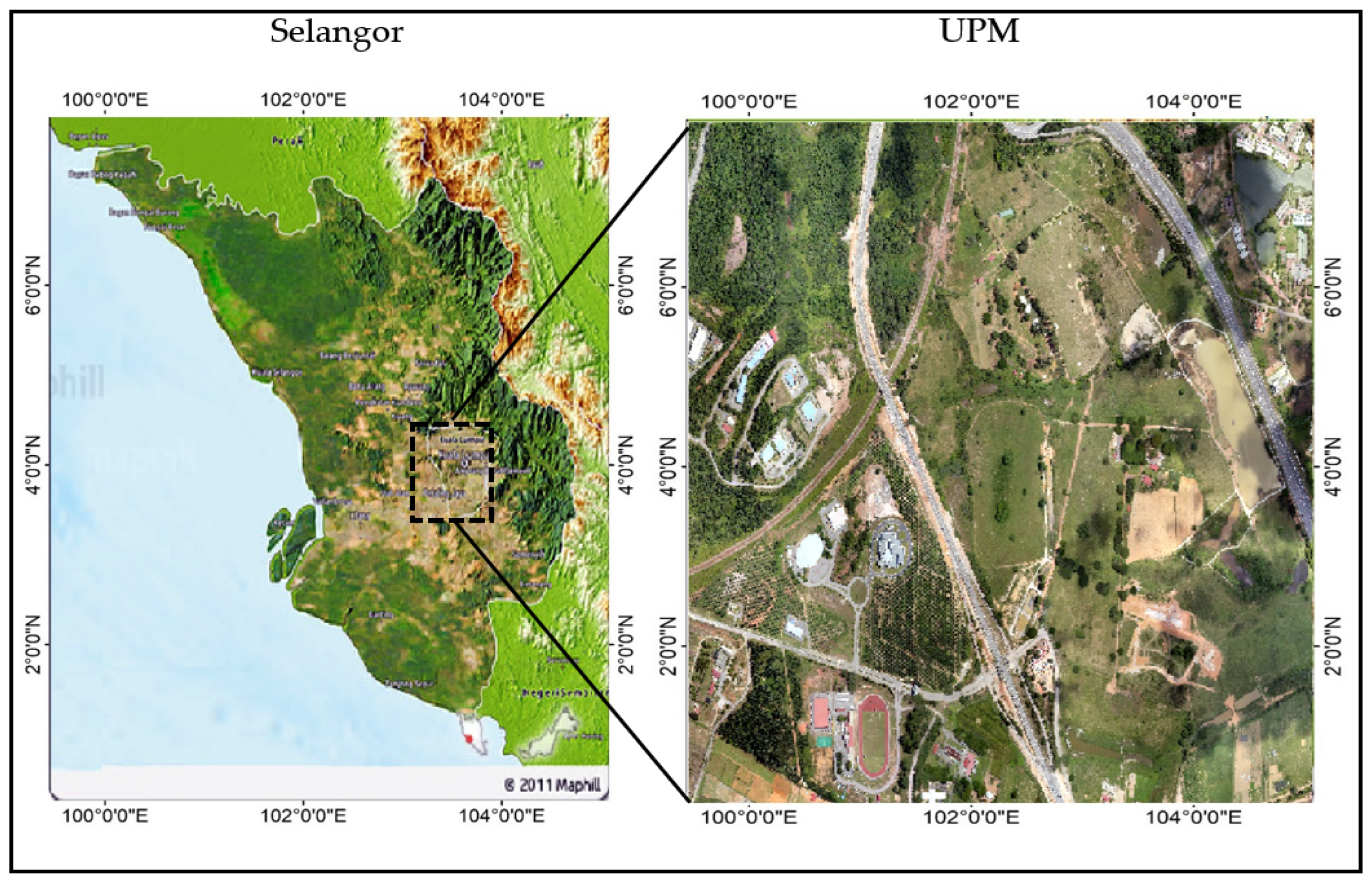
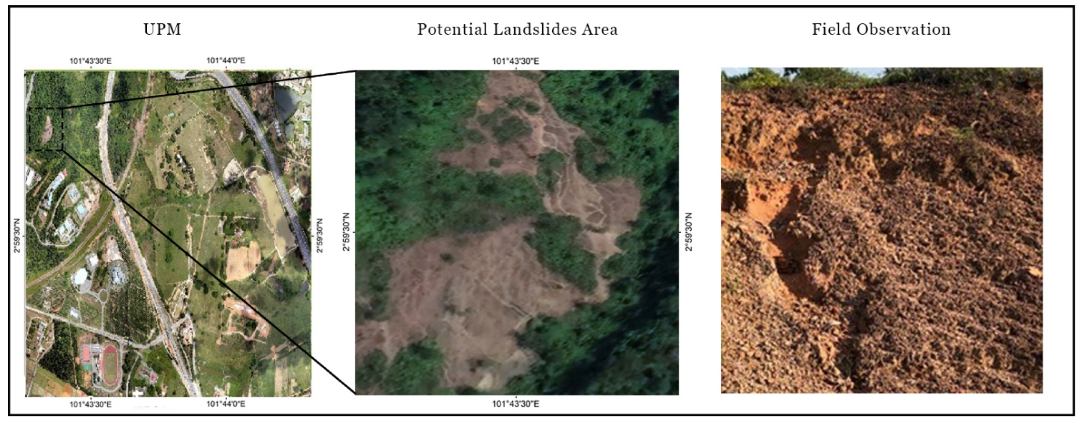
2.1. Study Area
2.2. Data
2.2.1. Landslide Conditioning Factors
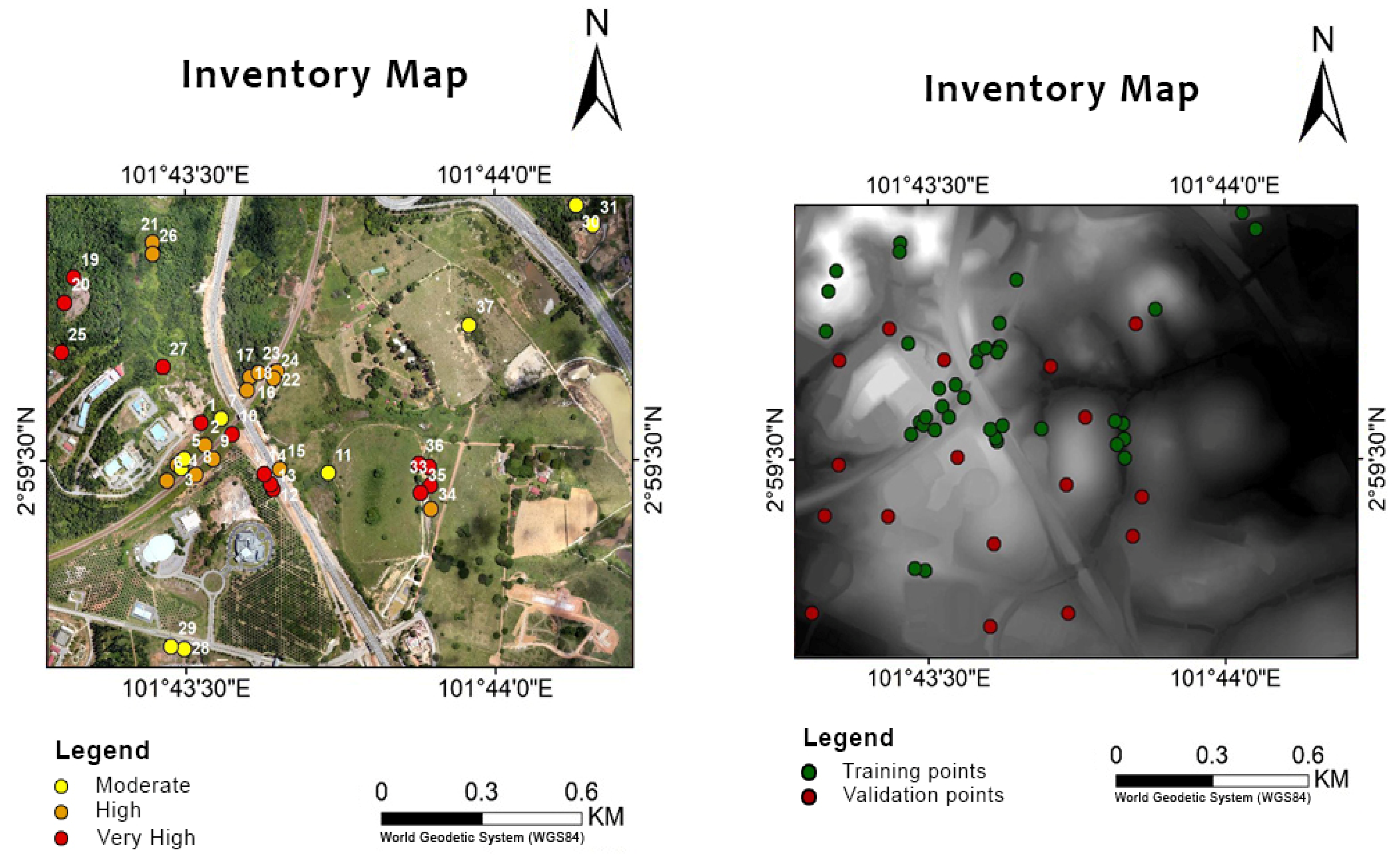
2.2.2. Landslide Inventory
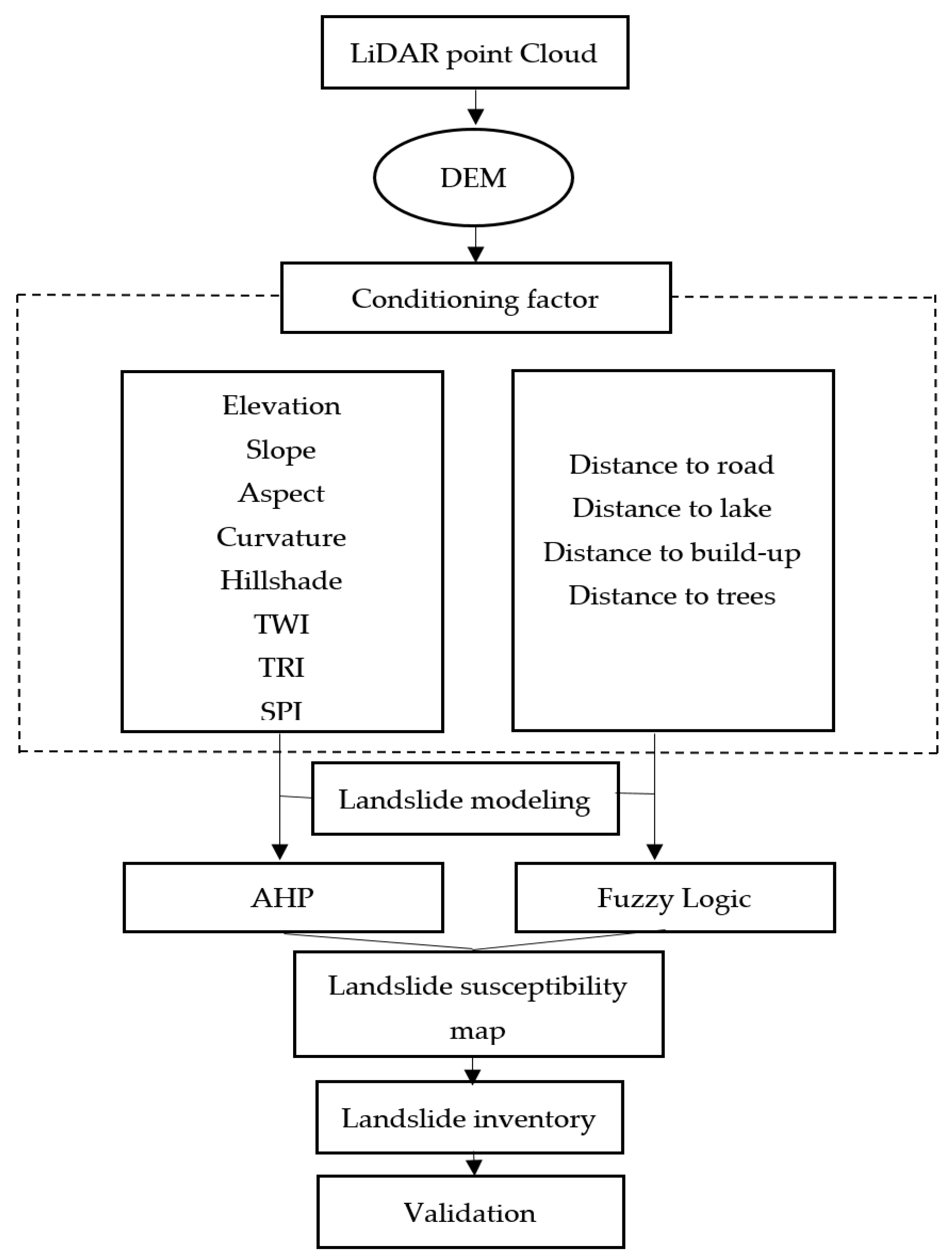
3. Methodology
3.1. Landslide Susceptibility Mapping (LSM)
3.2. Analytic Hierarchy Process (AHP)
3.3. Fuzzy Logic
3.4. Validation
4. Results
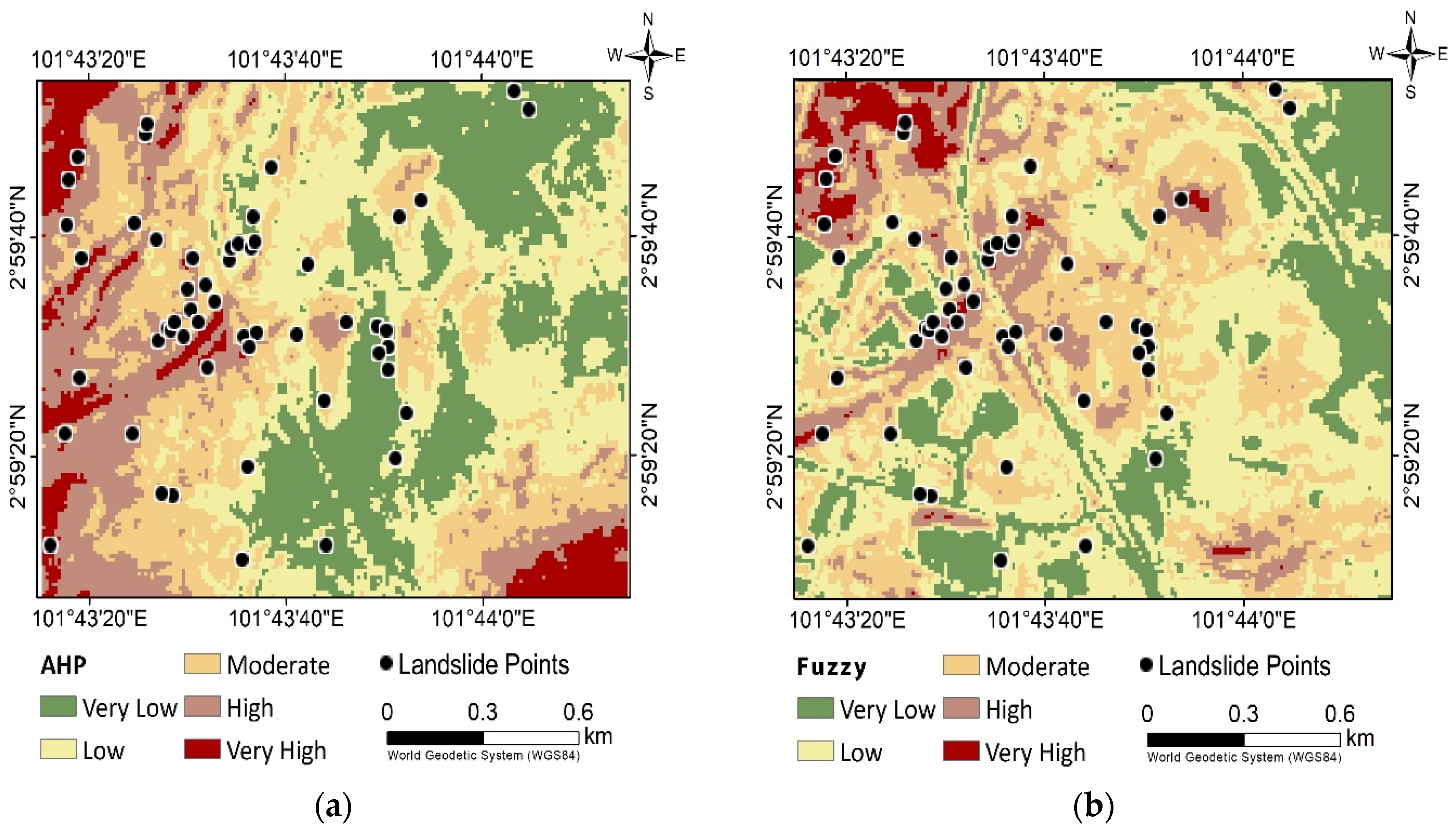
4.1. LSM by AHP
4.2. LSM by Fuzzy Logic
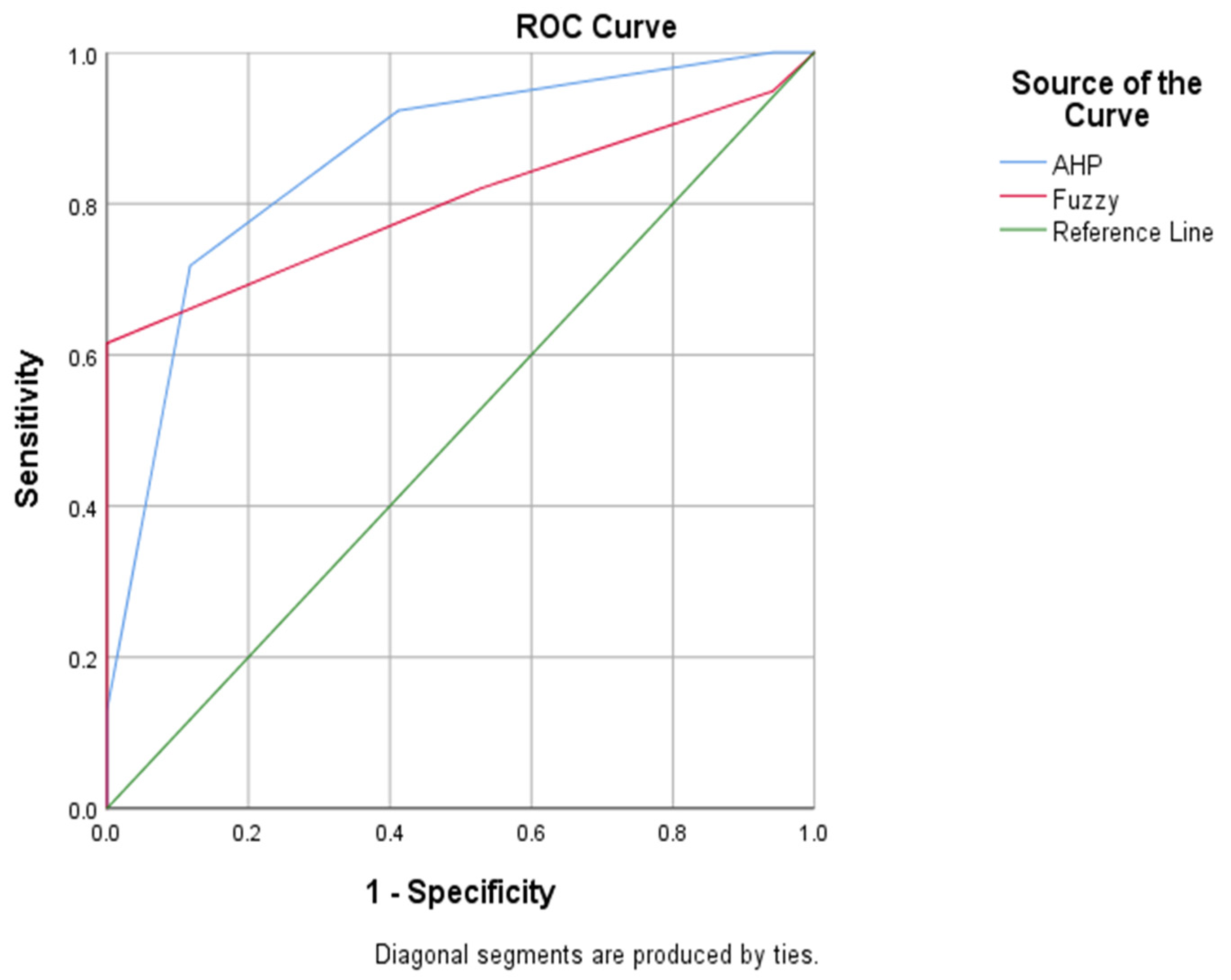
4.3. LSM Validation
5. Discussion
6. Conclusions
Author Contributions
Funding
Data Availability Statement
Conflicts of Interest
References
- Pradhan, B.; Sameen, M.I.; Kalantar, B. Ensemble Disagreement Active Learning for Spatial Prediction of Shallow Landslide; Springer: Cham, Switzerland, 2017; ISBN 9783319553429. [Google Scholar]
- Ahmad, J.; Lateh, H.; Saleh, S. Landslide Hazards: Household Vulnerability, Resilience and Coping in Malaysia. J. Educ. Hum. Dev. 2014, 3, 149–155. [Google Scholar] [CrossRef] [Green Version]
- Kalantar, B.; Ueda, N.; Lay, U.S.; Al-Najjar, H.A.H.; Halin, A.A. Conditioning Factors Determination for Landslide Susceptibility Mapping Using Support Vector Machine Learning. In Proceedings of the IEEE International Geoscience and Remote Sensing Symposium, Yokohama, Japan, 28 July–2 August 2019; pp. 9626–9629. [Google Scholar]
- Qi, T.; Zhao, Y.; Meng, X.; Chen, G.; Dijkstra, T. Ai-Based Susceptibility Analysis of Shallow Landslides Induced by Heavy Rainfall in Tianshui, China. Remote Sens. 2021, 13, 1819. [Google Scholar] [CrossRef]
- Psomiadis, E.; Papazachariou, A.; Soulis, K.X.; Alexiou, D.S.; Charalampopoulos, I. Landslide Mapping and Susceptibility Assessment Using Geospatial Analysis and Earth Observation Data. Land 2020, 9, 133. [Google Scholar] [CrossRef]
- Akter, A.; Noor, M.J.M.M.; Goto, M.; Khanam, S.; Parvez, A.; Rasheduzzaman, M. Landslide Disaster in Malaysia: An Overview. Int. J. Innov. Res. Dev. 2019, 8, 58–71. [Google Scholar] [CrossRef]
- Moradi, M.; Bazyar, M.H.; Mohammadi, Z. GIS-Based Landslide Susceptibility Mapping by AHP Method, a Case Study, Dena City, Iran. J. Basic Appl. Sci. Res. 2012, 2, 6715–6723. [Google Scholar]
- Pradhan, B.; Seeni, M.I.; Kalantar, B. Performance Evaluation and Sensitivity Analysis of Expert-Based, Statistical, Machine Learning, and Hybrid Models for Producing Landslide Susceptibility Maps; Springer: Cham, Switzerland, 2017; ISBN 9783319553429. [Google Scholar]
- Rahman, M.S.; Ahmed, B.; Di, L. Landslide Initiation and Runout Susceptibility Modeling in the Context of Hill Cutting and Rapid Urbanization: A Combined Approach of Weights of Evidence and Spatial Multi-Criteria. J. Mt. Sci. 2017, 14, 1919–1937. [Google Scholar] [CrossRef]
- Erener, A.; Düzgün, H.S.B. Landslide Susceptibility Assessment: What Are the Effects of Mapping Unit and Mapping Method? Environ. Earth Sci. 2012, 66, 859–877. [Google Scholar] [CrossRef]
- Najjar, H.A.H.A.; Pradhan, B.; Kalantar, B.; Sameen, M.I.; Santosh, M.; Alamri, A. Landslide Susceptibility Modeling: An Integrated Novel Method Based on Machine Learning Feature Transformation. Remote Sens. 2021, 13, 3281. [Google Scholar] [CrossRef]
- Roccati, A.; Paliaga, G.; Luino, F.; Faccini, F.; Turconi, L. Gis-Based Landslide Susceptibility Mapping for Land Use Planning and Risk Assessment. Land 2021, 10, 162. [Google Scholar] [CrossRef]
- Parise, M. Landslide Mapping Techniques and Their Use in the Assessment of the Landslide Hazard. Phys. Chem. Earth, Part C Solar, Terr. Planet. Sci. 2001, 26, 697–703. [Google Scholar] [CrossRef]
- Guzzetti, F.; Mondini, A.C.; Cardinali, M.; Fiorucci, F.; Santangelo, M.; Chang, K.T. Landslide Inventory Maps: New Tools for an Old Problem. Earth-Sci. Rev. 2012, 112, 42–66. [Google Scholar] [CrossRef]
- Quesada-román, A. Landslide Risk Index Map at the Municipal Scale for Costa Rica. Int. J. Disaster Risk Reduct. 2021, 56, 102144. [Google Scholar] [CrossRef]
- Quesada-Román, A.; Fallas-López, B.; Hernández-Espinoza, K.; Stoffel, M.; Ballesteros-Cánovas, J.A. Relationships between Earthquakes, Hurricanes, and Landslides in Costa Rica. Landslides 2019, 16, 1539–1550. [Google Scholar] [CrossRef]
- Santangelo, M.; Gioia, D.; Cardinali, M.; Guzzetti, F.; Schiattarella, M. Landslide Inventory Map of the Upper Sinni River Valley, Southern Italy. J. Maps 2015, 11, 444–453. [Google Scholar] [CrossRef] [Green Version]
- Batar, A.K.; Watanabe, T. Landslide Susceptibility Mapping and Assessment Using Geospatial Platforms and Weights of Evidence (WoE) Method in the Indian Himalayan Region: Recent Developments, Gaps, and Future Directions. ISPRS Int. J. Geo-Inf. 2021, 10, 114. [Google Scholar] [CrossRef]
- Al-Najjar, H.A.H.; Kalantar, B.; Pradhan, B.; Saeidi, V. Conditioning Factor Determination for Mapping and Prediction of Landslide Susceptibility Using Machine Learning Algorithms. In Proceedings of the Earth Resources and Environmental Remote Sensing/GIS Applications X, Strasbourg, France, 10–12 September 2019; Volume 11156, pp. 97–107. [Google Scholar] [CrossRef]
- Nohani, E.; Moharrami, M.; Sharafi, S.; Khosravi, K.; Pradhan, B.; Pham, B.T.; Lee, S.; Melesse, A.M. Landslide Susceptibility Mapping Using Different GIS-Based Bivariate Models. Water 2019, 11, 1402. [Google Scholar] [CrossRef] [Green Version]
- Kareem Jebur, A. Uses and Applications of Geographic Information Systems. Saudi J. Civ. Eng. 2021, 5, 18–25. [Google Scholar] [CrossRef]
- Aher, S.; Bairagi, S.I. Applications of Advanced Spaceborne Thermal Emission and Reflection Applications of Advanced Spaceborne Thermal Emission and Reflection. Online Int. Interdiscip. Res. J. 2014, 2, 2–14. [Google Scholar]
- Gesch, B.D.; Oimoen, M.; Greenlee, S.; Nelson, C.; Steuck, M.; Tyler, D. The National Elevation Dataset the National Elevation Dataset. J. Am. Soc. Photogramm. Remote Sens. 2015, 68, 5–32. [Google Scholar]
- Barbarella, M.; Fiani, M.; Lugli, A. Application of Lidar-Derived DEM for Detection of Mass Movements on a Landslide. Int. Arch. Photogramm. Remote Sens. Spat. Inf. Sci.-ISPRS Arch. 2013, 40, 89–98. [Google Scholar] [CrossRef] [Green Version]
- Wolock, D.M.; McCabe, G.J. Differences in Topographic Characteristics Computed from 100- and 1000-m Resolution Digital Elevation Model Data. Hydrol. Process. 2000, 14, 987–1002. [Google Scholar] [CrossRef]
- Tarboton, D.G. Terrain Analysis Using Digital Elevation Models in Hydrology. In Proceedings of the 23rd ESRI International Users Conference, San Diego, CA, USA, 6–9 July 2003; pp. 1–14. [Google Scholar]
- Lohani, B.; Ghosh, S. Airborne LiDAR Technology: A Review of Data Collection and Processing Systems. Proc. Natl. Acad. Sci. USA India Sect. A—Phys. Sci. 2017, 87, 567–579. [Google Scholar] [CrossRef]
- Mahalingam, R.; Olsen, M.J.; O’Banion, M.S. Evaluation of Landslide Susceptibility Mapping Techniques Using Lidar-Derived Conditioning Factors (Oregon Case Study). Geomatics, Nat. Hazards Risk 2016, 7, 1884–1907. [Google Scholar] [CrossRef]
- Haneberg, W.C.; Cole, W.F.; Kasali, G. High-Resolution Lidar-Based Landslide Hazard Mapping and Modeling, UCSF Parnassus Campus, San Francisco, USA. Bull. Eng. Geol. Environ. 2009, 68, 263–276. [Google Scholar] [CrossRef]
- Telbisz, T.; Látos, T.; Deák, M.; Székely, B.; Koma, Z.; Standovár, T. The Advantage of Lidar Digital Terrain Models in Doline Morphometry Compared to Topographic Map Based Datasets—Aggtelek Karst (Hungary) as an Example. Acta Carsologica 2016, 45, 5–18. [Google Scholar] [CrossRef]
- Brubaker, K.M.; Myers, W.L.; Drohan, P.J.; Miller, D.A.; Boyer, E.W. The Use of LiDAR Terrain Data in Characterizing Surface Roughness and Microtopography. Appl. Environ. Soil Sci. 2013, 2013, 13. [Google Scholar] [CrossRef]
- Schmid, K.A.; Hadley, B.C.; Wijekoon, N. Vertical Accuracy and Use of Topographic LIDAR Data in Coastal Marshes. J. Coast. Res. 2011, 27, 116–132. [Google Scholar] [CrossRef]
- Liu, X.; Zhang, Z.; Peterson, J.; Chandra, S. Large Area DEM Generation Using Airborne LiDAR Data and Quality Control. In Proceedings of the 8th International Symposium on Spatial Accuracy Assessment in Natural Resources and Environmental Sciences, Shanghai, China, 25–27 June 2008; pp. 79–85. [Google Scholar]
- Igwe, O.; John, U.I.; Solomon, O.; Obinna, O. GIS-Based Gully Erosion Susceptibility Modeling, Adapting Bivariate Statistical Method and AHP Approach in Gombe Town and Environs Northeast Nigeria. Geoenvironmental Disasters 2020, 7, 1–16. [Google Scholar] [CrossRef]
- Maskeliunaite, L.; Sivilevičius, H. Expert Evaluation of Criteria Describing the Quality of Travelling by International Passenger Train: Technological, Economic and Safety Perspectives. Technol. Econ. Dev. Econ. 2012, 18, 544–566. [Google Scholar] [CrossRef]
- Abdar, M.; Pourpanah, F.; Hussain, S.; Rezazadegan, D.; Liu, L.; Ghavamzadeh, M.; Fieguth, P.; Cao, X.; Khosravi, A.; Acharya, U.R.; et al. A Review of Uncertainty Quantification in Deep Learning: Techniques, Applications and Challenges. Inf. Fusion 2021, 76, 243–297. [Google Scholar] [CrossRef]
- Ghorbanzadeh, O.; Feizizadeh, B.; Blaschke, T. Multi-Criteria Risk Evaluation by Integrating an Analytical Network Process Approach into GIS-Based Sensitivity and Uncertainty Analyses. Geomat. Nat. Hazards Risk 2018, 9, 127–151. [Google Scholar] [CrossRef] [Green Version]
- Ghosh, S. Knowledge Guided Empirical Prediction of Landslide Hazard. Ph.D. Thesis, University of Twente, Enschede, The Netherlands, 2011. [Google Scholar]
- Norton, J. An Introduction to Sensitivity Assessment of Simulation Models. Environ. Model. Softw. 2015, 69, 166–174. [Google Scholar] [CrossRef]
- Guzzetti, F.; Reichenbach, P.; Ardizzone, F.; Cardinali, M.; Galli, M. Estimating the Quality of Landslide Susceptibility Models. Geomorphology 2006, 81, 166–184. [Google Scholar] [CrossRef]
- Shahabi, H.; Shirzadi, A.; Ghaderi, K.; Omidvar, E.; Al-Ansari, N.; Clague, J.J.; Geertsema, M.; Khosravi, K.; Amini, A.; Bahrami, S.; et al. Flood Detection and Susceptibility Mapping Using Sentinel-1 Remote Sensing Data and a Machine Learning Approach: Hybrid Intelligence of Bagging Ensemble Based on K-Nearest Neighbor Classifier. Remote Sens. 2020, 12, 266. [Google Scholar] [CrossRef] [Green Version]
- Pham, Q.B.; Achour, Y.; Ali, S.A.; Parvin, F.; Vojtek, M.; Vojteková, J.; Al-Ansari, N.; Achu, A.L.; Costache, R.; Khedher, K.M.; et al. A Comparison among Fuzzy Multi-Criteria Decision Making, Bivariate, Multivariate and Machine Learning Models in Landslide Susceptibility Mapping. Geomatics, Nat. Hazards Risk 2021, 12, 1741–1777. [Google Scholar] [CrossRef]
- Gutierrez, R.; Gibeaut, J.C.; Smyth, R.C.; Hepner, T.L.; Andrews, J.R.; Weed, C.; Mastin, M. Precise Airborne Lidar Surveying for Coastal Research and Geohazards Applications. Int. Arch. Photogramm. Remote Sens. 2001, 34, 22–24. [Google Scholar]
- Shano, L.; Raghuvanshi, T.K.; Meten, M. Landslide Susceptibility Evaluation and Hazard Zonation Techniques—A Review. Geoenvironmental Disasters 2020, 7, 1–19. [Google Scholar] [CrossRef]
- Nsengiyumva, J.B.; Luo, G.; Nahayo, L.; Huang, X.; Cai, P. Landslide Susceptibility Assessment Using Spatial Multi-Criteria Evaluation Model in Rwanda. Int. J. Environ. Res. Public Health 2018, 15, 243. [Google Scholar] [CrossRef] [Green Version]
- Toloie-Eshlaghy, A.; Homayonfar, M.; Aghaziarati, M.; Arbabiun, P. A Subjective Weighting Method Based on Group Decision Making for Ranking and Measuring Criteria Values. Aust. J. Basic Appl. Sci. 2011, 5, 2034–2040. [Google Scholar]
- Polykretis, C.; Ferentinou, M.; Chalkias, C. A Comparative Study of Landslide Susceptibility Mapping Using Landslide Susceptibility Index and Artificial Neural Networks in the Krios River and Krathis River Catchments (Northern Peloponnesus, Greece). Bull. Eng. Geol. Environ. 2014, 74, 27–45. [Google Scholar] [CrossRef]
- Saadatkhah, N.; Kassim, A.; Lee, L.M. Qualitative and Quantitative Landslide Susceptibility Assessments in Hulu Kelang Area, Malaysia. Electron. J. Geotech. Eng. 2014, 19, 545–563. [Google Scholar]
- Sulaiman, M.S.; Nazaruddin, A.; Salleh, N.M.; Abidin, R.Z.; Miniandi, N.D.; Yusoff, A.H. Landslide Occurrences in Malaysia Based on Soil Series and Lithology Factors. Int. J. Adv. Sci. Technol. 2019, 28, 1–26. [Google Scholar]
- Farooq Ahmed, M.; Rogers, J.D.; Ismail, E.H. A Regional Level Preliminary Landslide Susceptibility Study of the Upper Indus River Basin. Eur. J. Remote Sens. 2014, 47, 343–373. [Google Scholar] [CrossRef] [Green Version]
- Hinks, T.; Carr, H.; Gharibi, H.; Laefer, D.F. Visualisation of Urban Airborne Laser Scanning Data with Occlusion Images. ISPRS J. Photogramm. Remote Sens. 2015, 104, 77–87. [Google Scholar] [CrossRef] [Green Version]
- Hopkinson, C.; Chasmer, L. Using Discrete Laser Pulse Return Intensity to Model Canopy Transmittance. The Photogramm. J. Finland 2007, 20, 16–26. [Google Scholar]
- Bolstad, P.V.; Stowe, T. Evaluation of DEM Accuracy. Elevation, Slope, and Aspect. Photogramm. Eng. Remote Sens. 1994, 60, 1327–1332. [Google Scholar]
- Lakshmi, S.E.; Yarrakula, K. Review and Critical Analysis on Digital Elevation Models. Geofizika 2018, 35, 129–157. [Google Scholar] [CrossRef]
- Štular, B.; Lozić, E.; Eichert, S. Airborne LiDAR-Derived Digital Elevation Model for Archaeology. Remote Sens. 2021, 13, 1855. [Google Scholar] [CrossRef]
- Guzzetti, F.; Galli, M.; Reichenbach, P.; Ardizzone, F.; Cardinali, M. Landslide Hazard Assessment in the Collazzone Area, Umbria, Central Italy. Nat. Hazards Earth Syst. Sci. 2006, 6, 115–131. [Google Scholar] [CrossRef]
- Corominas, J.; Westen, C.J.V.; Frattini, P.; Fotopoulou, S. Recommendations for the Quantitative Analysis of Landslide Risk. Bull. Eng. Geol. Environ. 2014, 73, 209–263. [Google Scholar] [CrossRef] [Green Version]
- Beven, K.; Germann, P. Macropores and Water Flow in Soils Revisited. Water Resour. Res. 2013, 49, 3071–3092. [Google Scholar] [CrossRef] [Green Version]
- Arnone, E.; Dialynas, Y.G.; Noto, L.V.; Bras, R.L. Parameter Uncertainty in Shallow Rainfall-Triggered Landslide Modeling at Basin Scale: A Probabilistic Approach. Procedia Earth Planet. Sci. 2014, 9, 101–111. [Google Scholar] [CrossRef] [Green Version]
- Referee, A.; Carlo, M.; Comments, S.; Carlo, M. Interactive Comment on “Probabilistic Landslide Ensemble Prediction Systems: Lessons to Be Learned from Hydrology” by Ekrem Canli et Al. Nat. Hazards Earth Syst. Sci. Discuss 2018, 18, 2183–2202. [Google Scholar]
- Zawawi, A.A.; Shiba, M.; Jemali, N.J.N. Landform Classification for Site Evaluation and Forest Planning: Integration between Scientific Approach and Traditional Concept. Sains Malays. 2014, 43, 349–358. [Google Scholar]
- Arabameri, A.; Saha, S.; Roy, J.; Chen, W.; Blaschke, T.; Bui, D.T. Landslide Susceptibility Evaluation and Management Using Different Machine Learning Methods in the Gallicash River Watershed, Iran. Remote Sens. 2020, 12, 475. [Google Scholar] [CrossRef] [Green Version]
- Sharma, A.; Prakash, C. Evaluating the Impact of Road Construction on Landslide Susceptibility-A Case Study of Mandi District, Himachal Pradesh, India. Authorea Prepr. 2021, preprint, 1–14. [Google Scholar]
- Tanyaş, H.; Görüm, T.; Kirschbaum, D.; Lombardo, L. Could Road Constructions Be More Hazardous than an Earthquake in Terms of Mass Movement? Nat. Hazards 2022, 112, 639–663. [Google Scholar] [CrossRef]
- Pawluszek-Filipiak, K.; Oreńczak, N.; Pasternak, M. Investigating the E Ff Ect of Cross-Modeling in Landslide Susceptibility Mapping. Appl. Sci. 2020, 10, 6335. [Google Scholar] [CrossRef]
- Aslam, B.; Maqsoom, A.; Khalil, U.; Ghorbanzadeh, O.; Blaschke, T.; Farooq, D.; Tufail, R.F.; Suhail, S.A.; Ghamisi, P. Evaluation of Different Landslide Susceptibility Models for a Local Scale in the Chitral District, Northern Pakistan. Sensors 2022, 22, 3107. [Google Scholar] [CrossRef]
- Basheer, I.A.; Hajmeer, M. Artificial Neural Networks: Fundamentals, Computing, Design, and Application. J. Methods Microbiol. 2000, 43, 3–31. [Google Scholar] [CrossRef]
- Peng, C.; Wen, X. Recent Applications of Artificial Neural Networks in Forest Resource Management: An Overview Applications in Forest Resource Management; AAAI: Palo Alto, CA, USA, 1999. [Google Scholar]
- Haghbin, M.; Sharafati, A.; Motta, D.; Al-ansari, N. Applications of Soft Computing Models for Predicting Sea Surface Temperature: A Comprehensive Review and Assessment. Prog. Earth Planet. Sci. 2021, 9, 1–19. [Google Scholar] [CrossRef]
- Grant, M.J.; Booth, A. A Typology of Reviews: An Analysis of 14 Review Types and Associated Methodologies. Health Info. Libr. J. 2009, 26, 91–108. [Google Scholar] [CrossRef] [PubMed]
- Deng, X.; Li, L.; Tan, Y. Validation of Spatial Prediction Models for Landslide Susceptibility Mapping by Considering Structural Similarity. Int. J. Geo-Inf. 2017, 6, 103. [Google Scholar] [CrossRef] [Green Version]
- Westen, C.J.V.; Fonseca, F. International Society for Soil Mechanics And. In Proceedings of the SCG-XIII International Symposium on Landslides, Online, 22–26 February 2021. [Google Scholar]
- Dou, J.; Bui, D.T.; Yunus, A.P.; Jia, K.; Song, X.; Revhaug, I.; Xia, H.; Zhu, Z. Optimization of Causative Factors for Landslide Susceptibility Evaluation Using Remote Sensing and GIS Data in Parts of Niigata, Japan. PLoS ONE 2015, 10, e0133262. [Google Scholar] [CrossRef] [PubMed] [Green Version]
- Saaty, R.W. The Analytic Hierarchy Process-What It Is and How It Is Used. Math. Model. 1987, 9, 161–176. [Google Scholar] [CrossRef] [Green Version]
- Velasquez, M.; Hester, P. An Analysis of Multi-Criteria Decision-Making Methods. Int. J. Oper. Res. 2013, 10, 56–66. [Google Scholar]
- Nesticò, A.; Somma, P. Comparative Analysis of Multi-Criteria Methods for the Enhancement of Historical Buildings. Sustain. 2019, 11, 4526. [Google Scholar] [CrossRef] [Green Version]
- Zabihi, H.; Alizadeh, M.; Langat, P.K.; Karami, M.; Shahabi, H.; Ahmad, A.; Said, M.N.; Lee, S. GIS Multi-Criteria Analysis by Orderedweighted Averaging (OWA): Toward an Integrated Citrus Management Strategy. Sustainability 2019, 11, 1009. [Google Scholar] [CrossRef] [Green Version]
- Saaty, T.L. The Analytic Hierarchy Process. McGraw, New York. Agric. Econ. Rev. 1980, 70, 333. [Google Scholar]
- Jain, K. Site Suitability Analysis for Urban Development Using GIS. J. Appl. Sci. 2017, 7, 2576–2583. [Google Scholar] [CrossRef] [Green Version]
- Feizizadeh, B.; Shadman Roodposhti, M.; Jankowski, P.; Blaschke, T. A GIS-Based Extended Fuzzy Multi-Criteria Evaluation for Landslide Susceptibility Mapping. Comput. Geosci. 2014, 73, 208–221. [Google Scholar] [CrossRef] [PubMed] [Green Version]
- Vakhshoori, V.; Zare, M. Landslide Susceptibility Mapping by Comparing Weight of Evidence, Fuzzy Logic, and Frequency Ratio Methods. Geomatics, Nat. Hazards Risk 2016, 7, 1731–1752. [Google Scholar] [CrossRef]
- Baidya, P.; Chutia, D.; Sudhakar, S.; Goswami, C.; Goswami, J.; Saikhom, V.; Singh, P.S.; Sarma, K.K. Effectiveness of Fuzzy Overlay Function for Multi-Criteria Spatial Modeling—A Case Study on Preparation of Land Resources Map for Mawsynram Block of East Khasi Hills District of Meghalaya, India. J. Geogr. Inf. Syst. 2014, 06, 605–612. [Google Scholar] [CrossRef]
- Bamberger, S. Determining the Suitability of Yak-Based Agriculture in Illinois: A Site Suitability Analysis Using Fuzzy Overlay. Ph.D. Thesis, University of Southern California, Los Angeles, CA, USA, 2017. [Google Scholar]
- Aziz, R.S.; Khodakarami, L. Application of GIS Models in Site Selection of Waste Disposal in an Urban Area. WIT Trans. State Art Sci. Eng. 2013, 77, 27–35. [Google Scholar]
- ESRI. ESRI How Fuzzy Overlay Works; Environmental Systems Research Institute: Redlands, CA, USA, 1995. [Google Scholar]
- Pourghasemi, H.R.; Kariminejad, N.; Gayen, A.; Komac, M. Statistical Functions Used for Spatial Modelling Due to Assessment of Landslide Distribution and Landscape-Interaction Factors in Iran. Geosci. Front. 2020, 11, 1257–1269. [Google Scholar] [CrossRef]
- Mǎrgǎrint, M.C.; Grozavu, A.; Patriche, C.V. Assessing the Spatial Variability of Coefficients of Landslide Predictors in Different Regions of Romania Using Logistic Regression. Nat. Hazards Earth Syst. Sci. 2013, 13, 3339–3355. [Google Scholar] [CrossRef] [Green Version]
- He, H.; Hu, D.; Sun, Q.; Zhu, L.; Liu, Y. A Landslide Susceptibility Assessment Method Based on GIS Technology and an AHP-Weighted Information Content Method: A Case Study of Southern Anhui, China. ISPRS Int. J. Geo-Inf. 2019, 8, 266. [Google Scholar] [CrossRef] [Green Version]
- El Jazouli, A.; Barakat, A.; Khellouk, R. GIS-Multicriteria Evaluation Using AHP for Landslide Susceptibility Mapping in Oum Er Rbia High Basin (Morocco). Geoenvironmental Disasters 2019, 6, 1–12. [Google Scholar] [CrossRef]
- Ahmed, B. Landslide Susceptibility Mapping Using Multi-Criteria Evaluation Techniques in Chittagong Metropolitan Area, Bangladesh. Landslides 2015, 12, 1077–1095. [Google Scholar] [CrossRef] [Green Version]
- Fariza, A.; Abhimata, N.P.; Nur Hasim, J.A. Earthquake Disaster Risk Map in East Java, Indonesia, Using Analytical Hierarchy Process—Natural Break Classification. 2016 Int. Conf. Knowl. Creat. Intell. Comput. KCIC 2016 2017, 141–147. [Google Scholar] [CrossRef]
- Febrianto, H.; Fariza, A.; Hasim, J.A.N. Urban Flood Risk Mapping Using Analytic Hierarchy Process and Natural Break Classification (Case Study: Surabaya, East Java, Indonesia). In Proceedings of the 2016 International Conference on Knowledge Creation and Intelligent Computing (KCIC), Manado, Indonesia, 15–17 November 2016; pp. 148–154. [Google Scholar] [CrossRef]
- Gigović, L.; Drobnjak, S.; Pamučar, D. The Application of the Hybrid GIS Spatial Multi-Criteria Decision Analysis Best–Worst Methodology for Landslide Susceptibility Mapping. ISPRS Int. J. Geo-Inf. 2019, 8, 79. [Google Scholar] [CrossRef] [Green Version]
- Panchal, S.; Shrivastava, A.K. Landslide Hazard Assessment Using Analytic Hierarchy Process (AHP): A Case Study of National Highway 5 in India. Ain Shams Eng. J. 2022, 13, 101626. [Google Scholar] [CrossRef]
- Pourghasemi, H.R.; Pradhan, B.; Gokceoglu, C. Application of Fuzzy Logic and Analytical Hierarchy Process (AHP) to Landslide Susceptibility Mapping at Haraz Watershed, Iran. Nat. Hazards 2012, 63, 965–996. [Google Scholar] [CrossRef]
- Pham, B.T.; Khosravi, K.; Prakash, I. Application and Comparison of Decision Tree-Based Machine Learning Methods in Landside Susceptibility Assessment at Pauri Garhwal Area, Uttarakhand, India. Environ. Process. 2017, 4, 711–730. [Google Scholar] [CrossRef]
- Liu, Y.; Zhang, W.; Zhang, Z.; Xu, Q.; Li, W. Risk Factor Detection and Landslide Susceptibility Mapping Using Geo-Detector and Random Forest Models: The 2018 Hokkaido Eastern Iburi Earthquake. Remote Sens. 2021, 13, 1157. [Google Scholar] [CrossRef]
- Zhong, T.; Cang, X.; Li, R.; Tang, G. Landform Classification Based on Hillslope Units from DEMs. In Proceedings of the 30th Asian Conference on Remote Sensing (ACRS), Beijing, China, 18–23 October 2009; Volume 3, pp. 1686–1691. [Google Scholar]
- Kakavas, M.P.; Nikolakopoulos, K.G. Digital Elevation Models of Rockfalls and Landslides: A Review and Meta-Analysis. Geosciences 2021, 11, 256. [Google Scholar] [CrossRef]
- Lindsay, J.B.; Francioni, A.; Cockburn, J.M.H. LiDAR DEM Smoothing and the Preservation of Drainage Features. Remote Sens. 2019, 11, 1926. [Google Scholar] [CrossRef] [Green Version]
- Ciampalini, A.; Raspini, F.; Frodella, W.; Bardi, F.; Bianchini, S.; Moretti, S. The Effectiveness of High-Resolution LiDAR Data Combined with PSInSAR Data in Landslide Study. Landslides 2016, 13, 399–410. [Google Scholar] [CrossRef] [Green Version]
- Mahavir high (spatial) resolution vs. Low resolution Images. Int. Arch. Photogramm. Remote Sens. 2000, 33, 127–132.
- Vaze, J.; Teng, J. High Resolution LiDAR DEM—How Good Is It? In Proceedings of the MODSIM07—Land, Water and Environmental Management: Integrated Systems for Sustainability, Christchurch, New Zealand, 10–13 December 2007; pp. 692–698. [Google Scholar]
- Singh, H.; Huat, B.B.K.; Jamaludin, S. Slope Assessment Systems: A Review and Evaluation of Current Techniques Used for Cut Slopes in the Mountainous Terrain of West Malaysia. Electron. J. Geotech. Eng. 2008, 13, 1–24. [Google Scholar]
- Warren, S.D.; Hohmann, M.G.; Auerswald, K.; Mitasova, H. An Evaluation of Methods to Determine Slope Using Digital Elevation Data. Catena 2004, 58, 215–233. [Google Scholar] [CrossRef]


| Conditioning Factors | Calculation Approach | Influence on Terrain | Value Range |
|---|---|---|---|
| Elevation (m) | Derived directly from bare-earth LiDAR DEM | Captures the terrain climatic and vegetation growth characteristics | 34.668–105.560 |
| Slope (degree) | The maximum rate of change between cells in the elevation dataset and its neighbor cells. | Controls stress and strain in the soil, geomorphic process, and hydrology. | 0–83.365 |
| Aspect | By creating a map of the steepest downslope direction from each cell to its neighbors for an entire region | Aspect reveals the downslope direction of the maximum rate of change in value from an individual pixel to its neighbors | 0–359.900 |
| Plan Curvature | Through the calculation of the second derivative values of the terrain on a cell-by-cell basis as a fourth-order polynomial of the form. | Reveals the shape or curvature of the slope | Convex, flat, concave |
| Hillshade | Produced from surface raster putting illumination source angle and shadows into consideration | Uses the altitude and azimuth features to specify the position of the sun | 0–254.000 |
| TWI | From raster calculator for slope, flow direction, and flow accumulation from DEM. The value with 1 represents a flat area | Used to characterize spatial topographic diversity and complexity of landslide terrains and also to characterize landslides quantitatively | 1–9 |
| TRI | By focal statistics (maximum, minimum, and smooth) in the raster calculator. | Reveals terrain’s morphological heterogeneity, convergence and divergence of the flow of water, and topography discontinuity | 0.110–0.870 |
| SPI | By determining the flow accumulation at each cell. | Reveals the erosion potential from water flow, sediment yield, and concentration time. | 0–332.577 |
| Distance to road (m) | From Euclidean distance spatial analyst tool, and input feature source from the existing digitized roads on the area | This reveals the possibility that Landslides may occur on the slopes in proximity to the road as a result of modification by humans. Road constructions that modify the earth’s surface can impact landslide susceptibility [63,64]. | 0–602.000 |
| Distance to Lake (m) | Derived from spatial analyst’s Euclidean distance function and inputting water bodies as input feature source | Shows the effect of eroding or weathering of the lower part of the material, which causes the terrain to be weaker [65]. | 0–107.200 |
| Distance to build-up (m) | By inputting selected build-up features as the raster feature source in the analyst tool using the Euclidean distance function | Reveals the anthropogenic modification of the area, which reduces the tectonics of the slope | 0–505.000 |
| Distance to trees (m) | Using the Euclidean distance function and inputting the digitized trees feature as the raster source feature | Shows the possibility of vegetation roots anchoring the subsoil, which results in additional shear resistance that counters the destabilizing gravitational forces | 0–650.000 |
| S | E | H | C | A | DL | DT | TWI | TRI | DB | DR | SPI | |
|---|---|---|---|---|---|---|---|---|---|---|---|---|
| Slope (S) | 2 | 4 | 3 | 5 | 8 | 7 | 7 | 9 | 9 | 8 | 6 | |
| Elevation (E) | 1/2 | 3 | 3 | 4 | 6 | 6 | 5 | 8 | 8 | 8 | 4 | |
| Hillshade (H) | 1/4 | 1/3 | 1/2 | 2 | 5 | 4 | 3 | 6 | 7 | 6 | 2 | |
| Curvature (C) | 1/3 | 1/3 | 2 | 1 | 4 | 3 | 3 | 5 | 5 | 6 | 2 | |
| Aspect (A) | 1/5 | 1/4 | 1/2 | 1 | 3 | 2 | 2 | 5 | 5 | 5 | 1 | |
| D. Lake (DL) | 1/8 | 1/6 | 1/5 | 1/4 | 1/3 | 1/3 | 1/3 | 2 | 3 | 4 | 1/4 | |
| D. Trees (DT) | 1/7 | 1/6 | 1/4 | 1/3 | 1/2 | 3 | 1 | 4 | 6 | 5 | 1 | |
| TWI | 1/7 | 1/5 | 1/3 | 1/3 | 1/2 | 3 | 1 | 3 | 5 | 4 | 1/5 | |
| TRI | 1/9 | 1/8 | 1/6 | 1/5 | 1/5 | 1/2 | 1/4 | 1/3 | 2 | 2 | 1/6 | |
| D. Build-up (DB) | 1/9 | 1/8 | 1/7 | 1/5 | 1/5 | 1/3 | 1/6 | 1/5 | 1/2 | 1/2 | 1/7 | |
| D. Road (DR) | 1/8 | 1/8 | 1/6 | 1/6 | 1/5 | 1/4 | 1/5 | 1/4 | 1/2 | 2 | 1/9 | |
| SPI | 1/6 | 1/4 | 1/2 | 1/2 | 1 | 4 | 1 | 5 | 6 | 7 | 9 |
| Criteria | Membership Function |
|---|---|
| Elevation | Linear |
| Slope | Large |
| Aspect | Near |
| Curvature | Near |
| Hill shade | Linear |
| Distance to Lake | Linear |
| Distance to trees | Linear |
| Distance to Build up | Linear |
| Distance to Road | Linear |
| SPI | Large |
| TRI | Large |
| TWI | Large |
| Hazard Rating | Description | Implications |
|---|---|---|
| Very High | The event is expected to occur | Extensive investigation, planning, and implementation of treatment options are essential to reduce risk to acceptable levels |
| High | The event will probably occur under adverse conditions | Detailed investigation, planning, and implementation of treatment options essential to reduce risk to acceptable levels |
| Moderate | The event could occur under adverse conditions | It May be acceptable provided a treatment plan is implemented to maintain or reduce the risk level |
| Low | The event might occur under very adverse conditions | It can be accepted. Treatment to reduce risk levels should be defined |
| Very Low | The event is conceivable but only under exceptional circumstances | Accepted. Managed by routine procedures. |
Disclaimer/Publisher’s Note: The statements, opinions and data contained in all publications are solely those of the individual author(s) and contributor(s) and not of MDPI and/or the editor(s). MDPI and/or the editor(s) disclaim responsibility for any injury to people or property resulting from any ideas, methods, instructions or products referred to in the content. |
© 2023 by the authors. Licensee MDPI, Basel, Switzerland. This article is an open access article distributed under the terms and conditions of the Creative Commons Attribution (CC BY) license (https://creativecommons.org/licenses/by/4.0/).
Share and Cite
Okoli, J.; Nahazanan, H.; Nahas, F.; Kalantar, B.; Shafri, H.Z.M.; Khuzaimah, Z. High-Resolution Lidar-Derived DEM for Landslide Susceptibility Assessment Using AHP and Fuzzy Logic in Serdang, Malaysia. Geosciences 2023, 13, 34. https://0-doi-org.brum.beds.ac.uk/10.3390/geosciences13020034
Okoli J, Nahazanan H, Nahas F, Kalantar B, Shafri HZM, Khuzaimah Z. High-Resolution Lidar-Derived DEM for Landslide Susceptibility Assessment Using AHP and Fuzzy Logic in Serdang, Malaysia. Geosciences. 2023; 13(2):34. https://0-doi-org.brum.beds.ac.uk/10.3390/geosciences13020034
Chicago/Turabian StyleOkoli, Jude, Haslinda Nahazanan, Faten Nahas, Bahareh Kalantar, Helmi Zulhaidi Mohd Shafri, and Zailani Khuzaimah. 2023. "High-Resolution Lidar-Derived DEM for Landslide Susceptibility Assessment Using AHP and Fuzzy Logic in Serdang, Malaysia" Geosciences 13, no. 2: 34. https://0-doi-org.brum.beds.ac.uk/10.3390/geosciences13020034