Article

Landslide Susceptibility Modeling: An Integrated Novel Method Based on Machine Learning Feature Transformation

by
Husam A. H. Al-Najjar
1,
Biswajeet Pradhan
1,2,*,
Bahareh Kalantar
3,
Maher Ibrahim Sameen
1,
M. Santosh
4,5,6 and
Abdullah Alamri
7
1
Centre for Advanced Modelling and Geospatial Information Systems (CAMGIS), Faculty of Engineering and IT, University of Technology, Sydney, NSW 2007, Australia
2
Earth Observation Center, Institute of Climate Change, Universiti Kebangsaan Malaysia, Bangi 43600, Selangor, Malaysia
3
RIKEN Center for Advanced Intelligence Project, Goal-Oriented Technology Research Group, Disaster Resilience Science Team, Tokyo 103-0027, Japan
4
School of Earth Sciences and Resources, China University of Geosciences Beijing, Beijing 100083, China
5
Department of Earth Sciences, University of Adelaide, Adelaide, SA 5005, Australia
6
State Key Laboratory of Continental Dynamics, Department of Geology, Northwest University, Xi’an 710069, China
7
Department of Geology and Geophysics, College of Science, King Saud University, P.O. Box 2455, Riyadh 11451, Saudi Arabia
*
Author to whom correspondence should be addressed.
Remote Sens. 2021, 13(16), 3281; https://0-doi-org.brum.beds.ac.uk/10.3390/rs13163281
Submission received: 21 July 2021 / Revised: 11 August 2021 / Accepted: 17 August 2021 / Published: 19 August 2021

Abstract

:
Landslide susceptibility modeling, an essential approach to mitigate natural disasters, has witnessed considerable improvement following advances in machine learning (ML) techniques. However, in most of the previous studies, the distribution of input data was assumed as being, and treated, as normal or Gaussian; this assumption is not always valid as ML is heavily dependent on the quality of the input data. Therefore, we examine the effectiveness of six feature transformations (minimax normalization (Std-X), logarithmic functions (Log-X), reciprocal function (Rec-X), power functions (Power-X), optimal features (Opt-X), and one-hot encoding (Ohe-X) over the 11conditioning factors (i.e., altitude, slope, aspect, curvature, distance to road, distance to lineament, distance to stream, terrain roughness index (TRI), normalized difference vegetation index (NDVI), land use, and vegetation density). We selected the frequent landslide-prone area in the Cameron Highlands in Malaysia as a case study to test this novel approach. These transformations were then assessed by three benchmark ML methods, namely extreme gradient boosting (XGB), logistic regression (LR), and artificial neural networks (ANN). The 10-fold cross-validation method was used for model evaluations. Our results suggest that using Ohe-X transformation over the ANN model considerably improved performance from 52.244 to 89.398 (37.154% improvement).

Graphical Abstract

1. Introduction

Landslides are among the common natural disasters that cause considerable damage to life and property in various regions around the globe, with governments and other agencies having to spend a substantial amount to monitor and mitigate the disaster [1,2]. Although landslide-related damage cannot be entirely avoided, these events can be predicted to some extent so that damage to human life and property can be minimized [2]. In general, susceptibility maps are used to perform hazard and risk assessments in landslide-prone areas. Consequently, landslide susceptibility assessment has been considered as a fundamental step in landslide risk management. In recent years, machine learning (ML) methods have been widely adapted to evaluate diverse engineering and scientific problems, including in the field of geosciences. These methods have proved to yield a high level of accuracy to generate landslide susceptibility models [1,3]. Combining various types of machine learning (ML) models such as decision tree-based ensembles [4], integrating ML with geographic information systems (GIS) [5], and combining ML with different remote sensing data sources such as Interferometric Synthetic Aperture Radar (InSAR) [6], have also had a significant contribution to model improvements.
The ML methods provide promising solutions, particularly on a regional scale, even with limited geotechnical parameters [1]. However, in earlier studies, the default settings of the ML methods were used by assuming the normal distribution of the input data [7]. Yet, in landslide hazard studies, the variables might not normally be distributed, instead, they may have a Gaussian-like distribution (e.g., nearly Gaussian but with outliers or skewed) or a different distribution (e.g., exponential). Ideally, the majority of ML algorithms perform better when the input variables have a standard distribution form, as this provides an easier path for the algorithms to learn the weights of the parameters [8]. Moreover, it keeps beneficial information regarding the outliers and makes the algorithms less sensitive to them [9]. Thus, feature transformations [8], which are a part of feature engineering, can assist in fulfilling this aim. Feature engineering was initially established by George Box and David Cox to solve a situation involved with linear regression [10]. It happens in the pre-processing stage in ML before the primary modeling, providing a better understanding of the models’ behavior for the computer; however, it is a time-consuming part of learning in the projects [8]. Therefore, to achieve further robust modeling, most of the efforts in ML should be assigned to the pre-processing design/step [11,12]. This step has the potential to boost the learning scheme and the final output; more specifically, it was settled with the most recent advancements in the discipline of speech recognition [13,14] image processing [15] (e.g., in images dimension reduction or auto-encoders data) as well as diverse domains of science such as medical [16], biological [17], business, stock market [18], genetic [19], and information systems [20].
Numerous studies have been carried out in landslide susceptibility studies with respect to the different aspects of sampling methods [3,21], ML architecture [22], and validation measures [23]. Numerous studies have focused on sampling strategies, the selection of training samples, and addressing the effects of incomplete datasets [21,24]. Many studies have attempted to improve landslide susceptibility models by proposing new input factors into the process, including conditioning factors optimization [25,26]. For instance, researchers emphasized the comparison of different combinations of conditional factors, assuming the normal input for the analysis [27]. Other researchers have also developed techniques to assess the impacts of data resolution and scale [28], conditioning factors, data preparation methods for conditioning factors [7], and optimization techniques for statistically selecting the best factors [29]. As an example, scientists evaluated the effects of the spatial resolution of the digital elevation model (DEM) models and their products on landslide susceptibility mapping by considering the minimax normalization for the factor pre-processing [30]. Other researchers used ten continuous conditioning factors with an individual neuron for each variable, applying the common (minimax) normalization for the input variables [28]. Researchers also investigated the effects of factor optimization with artificial neural network (ANN) and logistic regression (LR) methods, concluding that the ANN method outperformed after optimization. Minimax transformation was utilized for the input, and the importance of such a processing step before modeling in landslide susceptibility was pointed out [31].
Furthermore, model parameterization and integration strategies have aided in improving landslide susceptibility mapping [32]. Statistical and ML models are often affected by the selection of proper hyper-parameters (parameterization) for a specific case study, and it has been extensively studied in the context of landslide susceptibility assessment. For example, researchers investigated various support vector machine (SVM) kernel functions for the input, including linear, polynomial, radial, and sigmoid functions, in which the radial showed the best performance compared to the other functions [32]. A comprehensive study in the Cameron Highlands, Malaysia, evaluated the performance and sensitivity analysis of various ML techniques such as the expert-based, statistical, and hybrid models. The type of pre-processing used in their study was mostly focused on removing the noise, the selection of the most important conditioning factors, and the conventional data normalization for the input [7]. Scholars implemented the powerful Gaussian function for the input and the susceptibility maps were generated based on the decision tree (DT), SVM, and adaptive neuro-fuzzy inference systems (ANFIS) in Penang, Malaysia [33].
Improving landslide modeling through ensemble strategies has also been an active research field in landslide studies. The ensemble techniques performed well in generalizing compared with other previous methods of ANN, SVM, and Naïve Bayes (NB) applied to the same study area; however, these studies utilized the default form for feeding the data [30]. Researchers used the minimax normalization scalar for their modeling and reported that the ANN model outperformed the previous extreme gradient boosting (XGB) model for the same study area. However, limited conditioning factors and inventories were the main drawbacks of their study [34].
More recently, the performance of several MLs, such as the backpropagation neural network (BPNN), one-dimensional convolutional neural network (1D-CNN), DT, random forest (RF), and XGB, was extensively assessed by [35]. In their study, the imbalance in the dataset was eliminated, and the normal distribution for ML models was used. Their result showed that XGB had peak accuracy among the other models. They reported that the pre-processing data workload had a significant impact on the classifier. In multi-hazard modeling (including landslides) various ML methods were designed and assessed using 21 conditional hazard factors [36]. The normalized default of the input was used, and SVM was reported as the most accurate model for predicting landslides. In another study, ref. [37] utilized the normal distribution setting of ML and the Logistic Model Tree model had the highest accuracy followed by LR, NB, ANN, and SVM, respectively.
As evident from the various studies mentioned above, the quality of the training is a crucial element in determining the accuracy and generalization of landslide models. In ML, some methods, i.e., based on the distance between data points, such as k-nearest neighbors (KNN), SVM, or ANN, prefer the input variables to be normalized to gain the best practice of modeling. Previous studies significantly improved the landslide models using different approaches, such as data-dependent methods [24,38], diverse architectures [22,33], and training strategies [39,40]. Nevertheless, they used the conventional process of data, e.g., feature normalization, and none of those studies have reported the effect of different feature transportation on model performance.
Therefore, the current study aims to assess the effectiveness of six feature transformations, including minimax normalization (Std-X), logarithmic functions (Log-X), reciprocal function (Rec-X), power functions (Power-X), optimal features (Opt-X) selected by random forest, and one-hot encoding (Ohe-X) applied to land use and vegetation density on landslide susceptibility by applying them on three models, namely XGB, LR, and ANN as benchmark models. Initially, 11 conditioning factors (including continuous and categorical factors) and 35 landslide locations were used. The techniques were evaluated by 10-fold cross-validation and receiver operating characteristic (ROC) curves within a region in the Cameron Highlands in Malaysia.

2. Study Area and Dataset
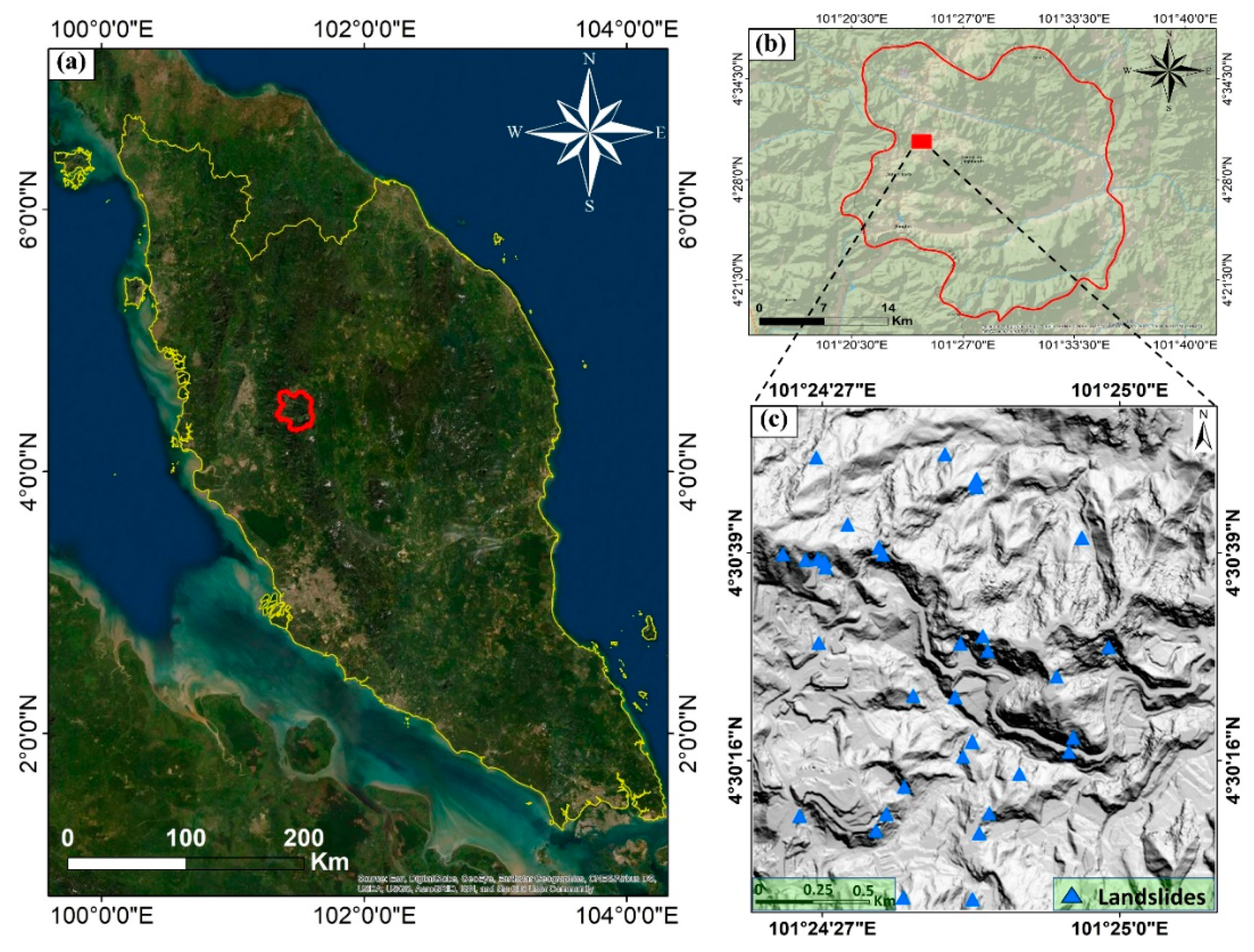
2.1. Study Area

The study area was chosen in a tropical area in the Cameron Highlands in the state of Pahang, Malaysia (Figure 1). This region has experienced numerous landslides and floods in the past, which were mainly caused by heavy and prolonged rainfall [2]. The predominant land cover of the area is a rainforest with dense vegetation. The geographic location of the area is between latitude 101°24′00″ E and 101°25′10″ E and longitude 4°30′00″ N and 4°30′55″ N. The mean annual rainfall in this region is 2660 mm. The day and night average temperatures are 24 °C and 14 °C, respectively. Geographically, the area is hilly, with elevation ranging from 1451.92 to 1838.23 m. The dominant lithology of the area is composed of granites, phyllite, and some schists layers [3].

2.2. Dataset

2.2.1. Landslide Inventory

Landslide susceptibility assessment requires landslide inventories for the training and validation of models. The inventories can be prepared through field surveys, past landslide events from news and government records, and remote sensing data. In this research, a landslide inventory identified 35 landslide locations (shallow landslides) in the Cameron Highlands, Malaysia (Figure 1), taken from the previous projects [2,3,29,41].
In addition, the light detection and ranging (LiDAR) data was used to derive the DEM over a 25 km2 area, and other associated conditioning parameters. The data was captured on the 15th of January 2015 using an airborne laser scanning system (RIEGL) with a point spacing of 8 points per square meter and an altitude of 1510 m [2,42].
The DEM was formed with 0.5-m spatial resolution from the last return LiDAR point clouds, and it was derived using the ArcGIS Pro based on the multiscale curvature method (curvature filtering technique) [43]. In addition, the inverse distance weighting interpolation technique was used to convert the point clouds into a raster format.

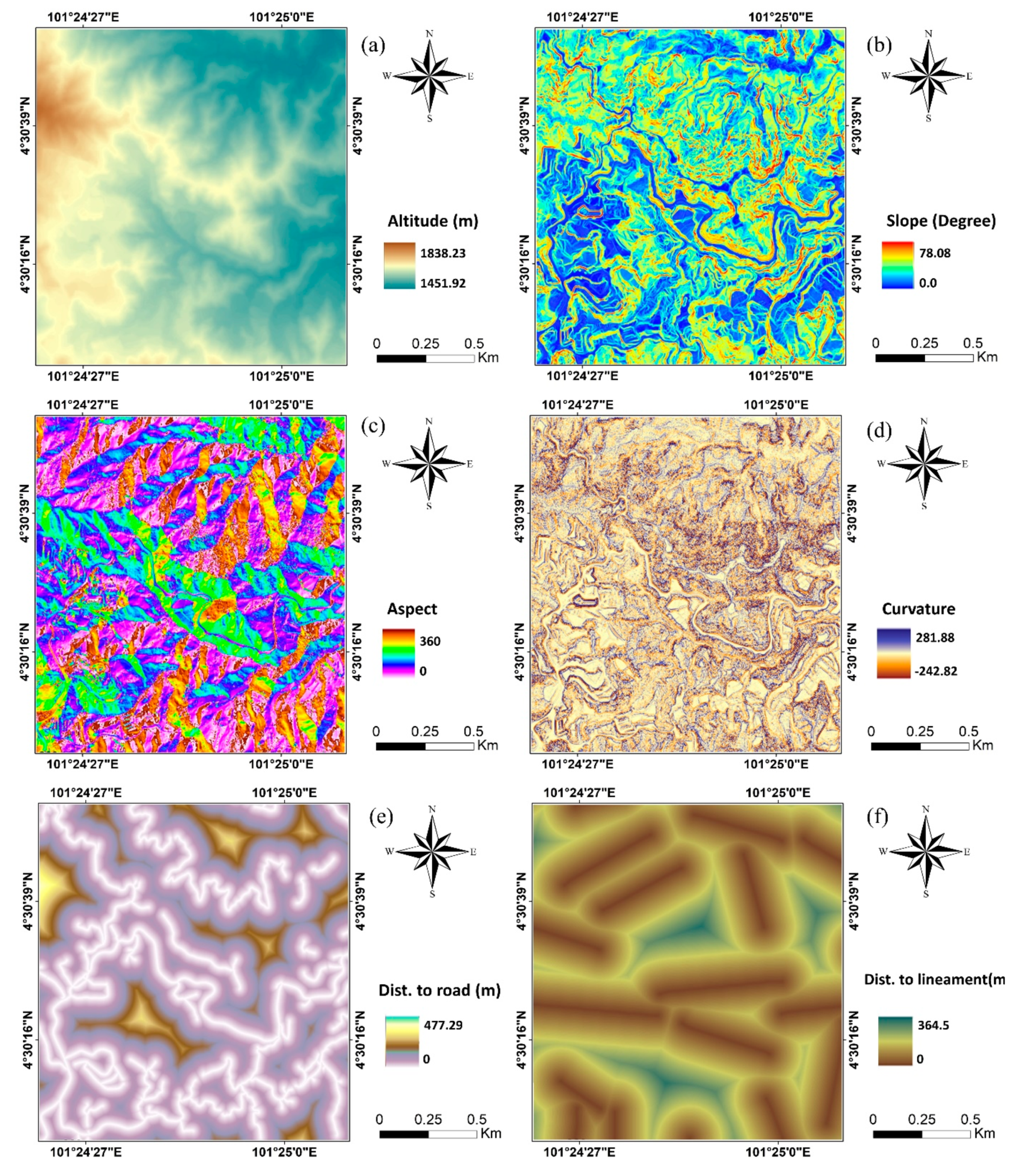
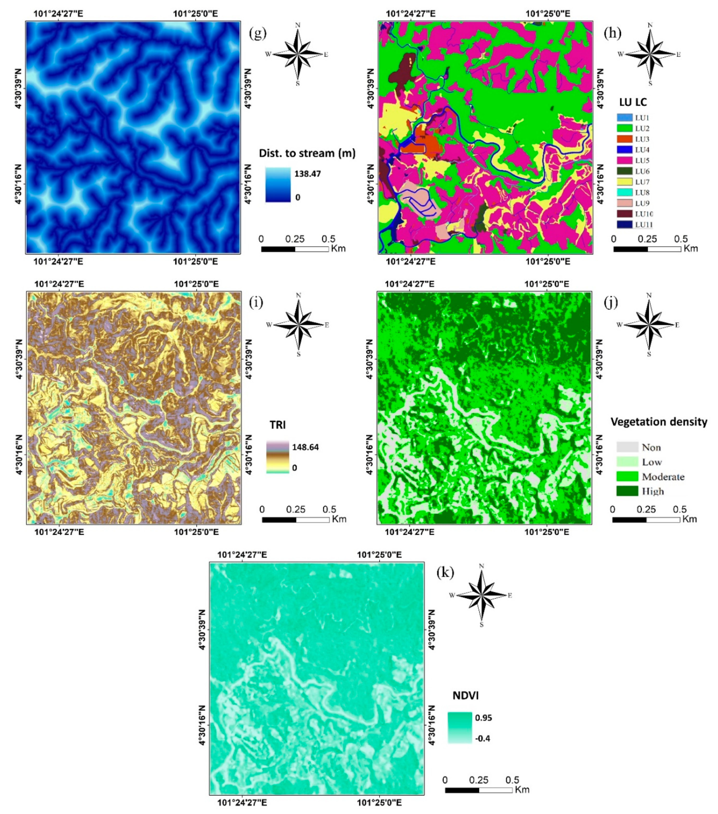
2.2.2. Landslide Conditioning Factors

Altitude, slope, aspect, curvature, distance to road, distance to lineament, distance to stream, land use and land cover, terrain roughness index (TRI), vegetation density, and the normalized difference vegetation index (NDVI) were used as geo-environmental factors due to the wide usage of these parameters in a large number of landslide susceptibility studies [33]. The effectiveness and functionality of each conditioning factor are provided in the following:
Altitude: variation in the elevation considerably influences the mapping of landslide susceptibility [30]. In the study area, the altitude varies between 1451.92 and 1838.23 m (Figure 2a);
Slope: Slope is one of the key parameters leading to soil instability, especially in extreme conditions. Generally, while the slope increases, the strength capacity of the soil decreases [44]. In this research, the slope of the investigation region was in the 0–70.08 degrees range (Figure 2b);
Aspect: It represents the downslope direction of the maximum rate of change in value from each cell to its neighbors (slope direction). It can also indicate specific measures for soil moisture, evaporation, and distribution of vegetation that requires large quantities of moisture [45]. It varies from 0 to 360 degrees (Figure 2c);
Curvature: The ground shape of the earth with the corresponding runoff is identified as surface curvature. It has a critical role in changing the characteristics of landforms. Thus, it is an important factor for landslide modeling. The convex surface instantly drains wetness, while for an extended duration, the concave surface keeps humidity [46]. The curvature (total curvature) is a combination of profile curvature (parallel direction with maximum slope) and plan curvature (perpendicular to the orientation of maximum slope). In this work, the curvature ranges from −242.82 degrees to 281.88 degrees (Figure 2d);
Distance to road: Excavations, the application of external loads, and the eviction of plants are common activities during construction along highways and roads. These occasions might be a direct or indirect impact of human activities and soil erosion in prone areas. The likelihood of landslide events is generally increased with the distance to road, stream, and lineament. The Euclidean distance analysis is used to generate these layers [44] (Figure 2e);
Distance to lineament: The geology of the area can be strongly affected by faults, fractures, and joints, providing ideal pathways for drainage and, therefore, the proximity to lineament has an influential impact on landslide occurrence [47] (Figure 2f);
Distance to stream: Furthermore, distance to stream as a raster layer was derived from the DEM utilizing the Euclidean distance analysis and existing topographic map of the study area [30] (Figure 2g);
Land use land cover: Human activities are also considered influential on landslides because they affect patterns of land use and land cover. The land use map of the study was taken from the department of the survey and mapping in Malaysia in the same year [30]. Eleven classes in the study area were identified as categorical classes, namely LU1: Water; LU2: Forest; LU3: Industrial; LU4: Infrastructure; LU5: Agriculture; LU6: Residential; LU7: Vacant; LU8: Transportation; LU9: Facilities; LU10: Mixed; LU11: Commercial (Figure 2h);
Terrain Roughness Index (TRI): TRI is one of the essential hydrological factors that contribute to identifying landslide-prone areas. It illustrates the changes in the height of adjacent cells in a DEM and affects the topographic and hydrological processes in the development of landslide events [44]. In the current study, the TRI values range from 0 to 148.64 (Figure 2i). The TRI was calculated using Equation (1) [45]:
T R I = m a x 2 m i n 2
where, min and max values represent the highest and lowest number of rectangular cells within nine DTM windows, respectively;
Normalized Difference Vegetation Index (NDVI): This index was extracted from a high-resolution SPOT 5 image (10 m) by applying the band ratio in Equation (2). The output of the NDVI raster (Figure 2j) often ranges from −1 to 1, where the negative rates imply non-vegetated regions and the high positive rates demonstrate a good condition of green vegetation [7]:
N D V I = N I R R E D ( N I R + R E D )
Vegetation density: Vegetation density, as a categorical conditioning factor, was determined using the NDVI index, which was reclassified by the quantile classification method in the ArcGIS Pro. The NDVI raster was then reclassified using the manual classification method into four classes with a range of values: (−1 to −0.5) as non-vegetation; (−0.51 to 0) as low density; (0.1 to 0.5) as moderate density; (0.51 to 1) as high density [7] (Figure 2k).

3. Methods

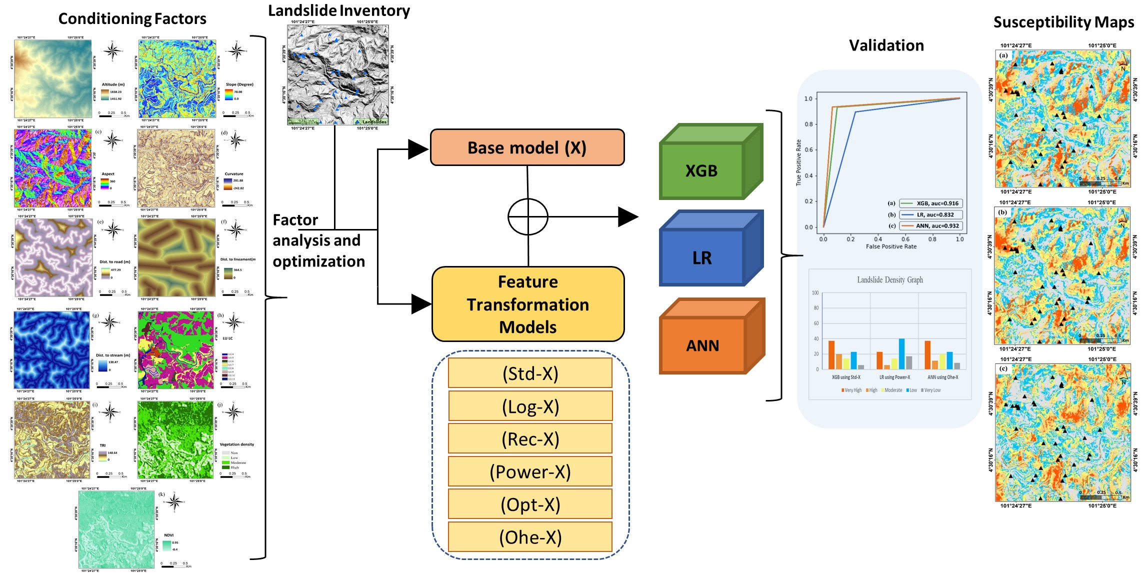
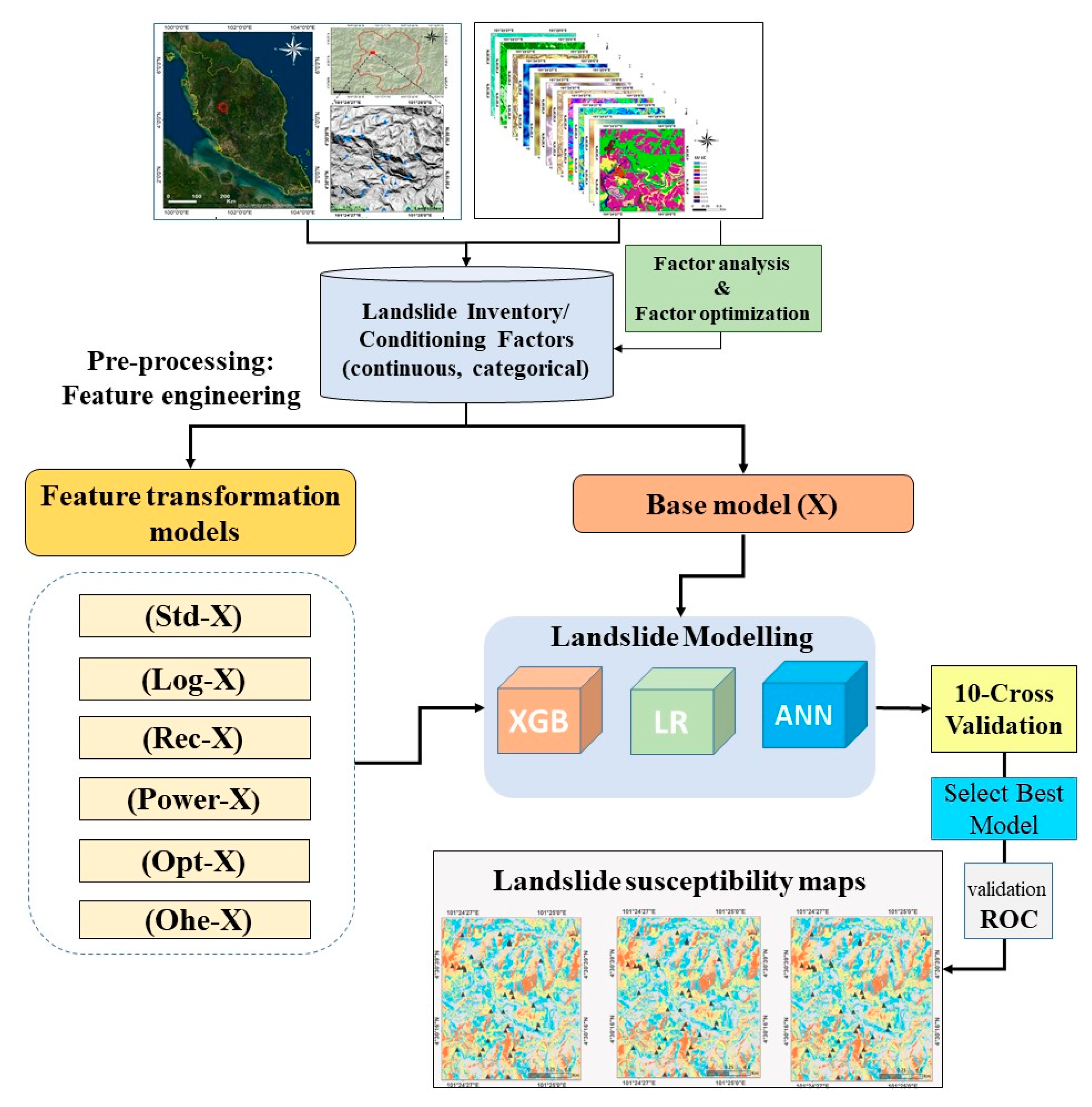
3.1. Overall Workflow

The overall workflow of the current study is shown in Figure 3. Initially, 11 conditioning factors (nine continuous factors and two categorical) were selected as input variables. Among them, ten influential conditioning factors (NDVI excluded) were set by considering the multicollinearity analysis based on previous research [3,7].
Moreover, 35 landslide (and 35 random non-landslide) events were identified to feed the models. Six feature transformation models, along with the base model, were considered for the landslide susceptibility assessment. Three benchmark algorithms from different ML families (i.e., XGB, LR, ANN) were chosen to assess which model obtains the benefits from the transformations. To evaluate and further reduce the effect of over/under promising prediction, 10-fold cross-validations were implemented. This validation can minimize the impact of over/under promising prediction results. Finally, three landslide susceptibility maps were produced and evaluated according to the highest accuracy models in each ML group.

3.2. Feature Transformations

Feature transformation is the process of modifying data but maintaining the information. These modifications can make understanding ML algorithms easier, delivering better outcomes by improving the performance and data integrity. In data points, for example, replacing a variable or feature “ x ” by a function of x (e.g., log x ) is a type of feature transformation [48]. The transformed feature will then be used as input to run models.
Feature transformation is a part of feature engineering. Feature engineering is a skill that extracts further information from the existing data. It does not add any data, but it makes the data more useful for ML models to learn and understand the models [8]. Feature engineering can be divided into two main stages, namely feature transformation and feature creation. The transformation refers to a process that replaces the distribution of a variable with others [48]. In contrast, the feature creation technique is an approach to create new features (variables) based on the existing variables [49]. In this study, the feature transformation technique was applied to the landslide conditioning factors as specific variables. The type of functions used for the transforming process is provided in Table 1. It describes the functionality of six transformations [50,51] used in the current study.

3.3. Modeling Methods

3.3.1. Extreme Gradient Boosting (XGB)

In the case of a small to medium range of data, decision tree-based methods are identified as one of the cutting-edge techniques. As such, the new popular tree-based boosting method is XGB, which has gained a great deal of attention in the latest studies [59,60,61]. Initially, it was introduced as a research project in 2016 as a scalable boosting system [59]. The prediction ability of XGB is high because the weightage is based on unexpected errors coming from the training process. This method utilizes distributed and parallel evaluation in data mining, such as classification, regression, and ranking. It offers a great advantage over the other methods by providing optimal usage of memory and low computational cost [62,63,64]. Moreover, Bayesian optimization constructs an influential approach for parameter optimization in XGB [60]. Considering K observations and P features for a specific dataset; H = { ( X i ,   Y i ) }   ( | H | = k ,   X i     R p   ,   Y i     R ) . The result of a tree ensemble model can be evaluated for M   additive functions as the following:
Y i =   ( X i ) = m = 1 M f m   ( X i ) ,   f m   S ,
where, a regression tree space is denoted as F , it is determined using the following equation:
S = { f ( x ) = w b ( x ) }   ( b :   R p   T ,   w R T ) ,
where, b   represents the framework of the tree,   T represents tree leaves, and f m is a function of b , and leaf weight is w . To reduce errors in the tree, the reduction function is computed in the XGB as below:
L ( t ) = k = 1 k l ( Y i Y ^ i t 1 + f t   ( X i ) ) + Ω ( f t ) ,
where ,   l is denoted as a dissimilar function of convex objective, resolving the error between measured ( Y ^ i ) and estimated values of ( Y i ); t is iteration for lessening the errors, and Ω is the regression tree complicatedness:
Ω   ( f k ) = γ T + 1 2 γ | | w | | 2
Generally, using a more regulated interpretation to limit overfitting problems makes the XGB as a unique and high-performance technique. It can be separated into three categories, namely, General Parameters, Task Parameters, and Booster Parameters [59]. In the present study, three common parameters were selected in XGB for landslide susceptibility application, Colsample_bytree (subsample ratio of columns when constructing each tree), Subsample (subsample ratio of the training instance), and Nrounds (max number of boosting iterations).

3.3.2. Logistic Regression (LR)

LR models are used to model the likelihood of a particular event or class, such as landslide/non-landslide events [65]. It categorizes the correlation between a variable and some dependent parameters, including binary, continuous, or categorical. No need for having normal distribution is one of the main advantages of LR models [42]. Independent variables can be assigned to 0 and 1, representing the existence or non-existence of landslide events. The outcome of the model ranges between 0 and 1, which indicates the landslide susceptibility. The logistic function is the basis of this model, which can be computed by Equation (7) [66]:
Y = 1 1 + e ( α + β 1 x 1 + β 2 x 2 + β n x n )
where, α is a constant number, n represents the number of independent numbers, X i ( i = 1 , 2 ,   ,   n ) denotes the variables of the predictor, and β i   ( i = 1 , 2   , 3 , ,   n ) represents the LR coefficient.

3.3.3. Artificial Neural Networks (ANN)

ANNs involve higher complexity in their design, hidden layers, and neutrons, compared with XGB models. The architecture of this model forms a set of neurons, initiated with an input layer, in which the required parameters can be entered for training, testing, and validating. The intermediate or hidden layers are located after the input layer, which are responsible for learning the complex function to extract the major features from input examples [67]. These hidden layers are responsible for landslide susceptibility measurements for a given pixel on a scale, resulting in ranges from low to high susceptibility (range from 0 to 1) [68].
Feedforward neural networks (Figure 4) are the most widely used network architecture, which is accepted as a useful neural network for landslide susceptibility [42]. Such a model is made of layers with an input layer to receive information, an output layer to transmit information to hidden layers, and the latter act as a feature extractor. The information in the input layer propagates to the next hidden layer. Hidden layers get weighted sums of incoming signals and process them using an activation function, most commonly sigmoid and hyperbolic tangent functions. In turn, hidden units send output signals to the next layer. This layer can either be another hidden layer or the output one. Information is propagated forward until the network produces output.

3.4. Evaluation Metrics

3.4.1. The 10-Fold Cross-Validation

Cross-validation is commonly used to evaluate the generalization of the prediction, avoiding the over-promising/under-promising predictions. It acts as a repeated random sub-sampling technique that no two test sets interfered with. The learning set is split up into a K-separated subset of almost equivalent size (fold). The training process is performed utilizing a subset of K-1 fold as the first training set, then the model is learned over the rest of the subsets. This process is repeated until every one of the K-folds has been filled as a validation set. The performance is then computed as an average of all K-fold executions [69]. In the current study, the average accuracy was computed 10-fold.

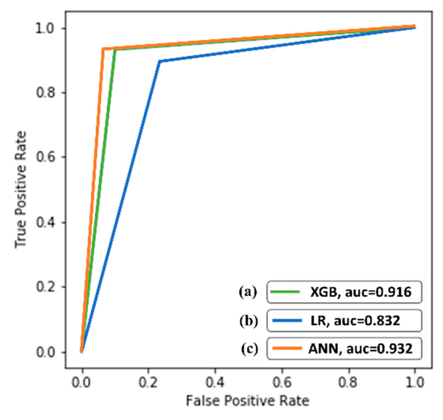
3.4.2. Receiver Operating Characteristics (ROC)

The landslide susceptibility analysis was performed using the receiver operating characteristics (ROC) curve, where the true positive rate is plotted counter to the false positive rate at some threshold settings. In landslide susceptibility analysis, the AUC defines the accuracy of the engaged model. The range of the AUC begins from 0.5 to 1, where 0.5 indicates weak performance, while a value of 1 denotes the ideal performance of a model [33].

4. Results

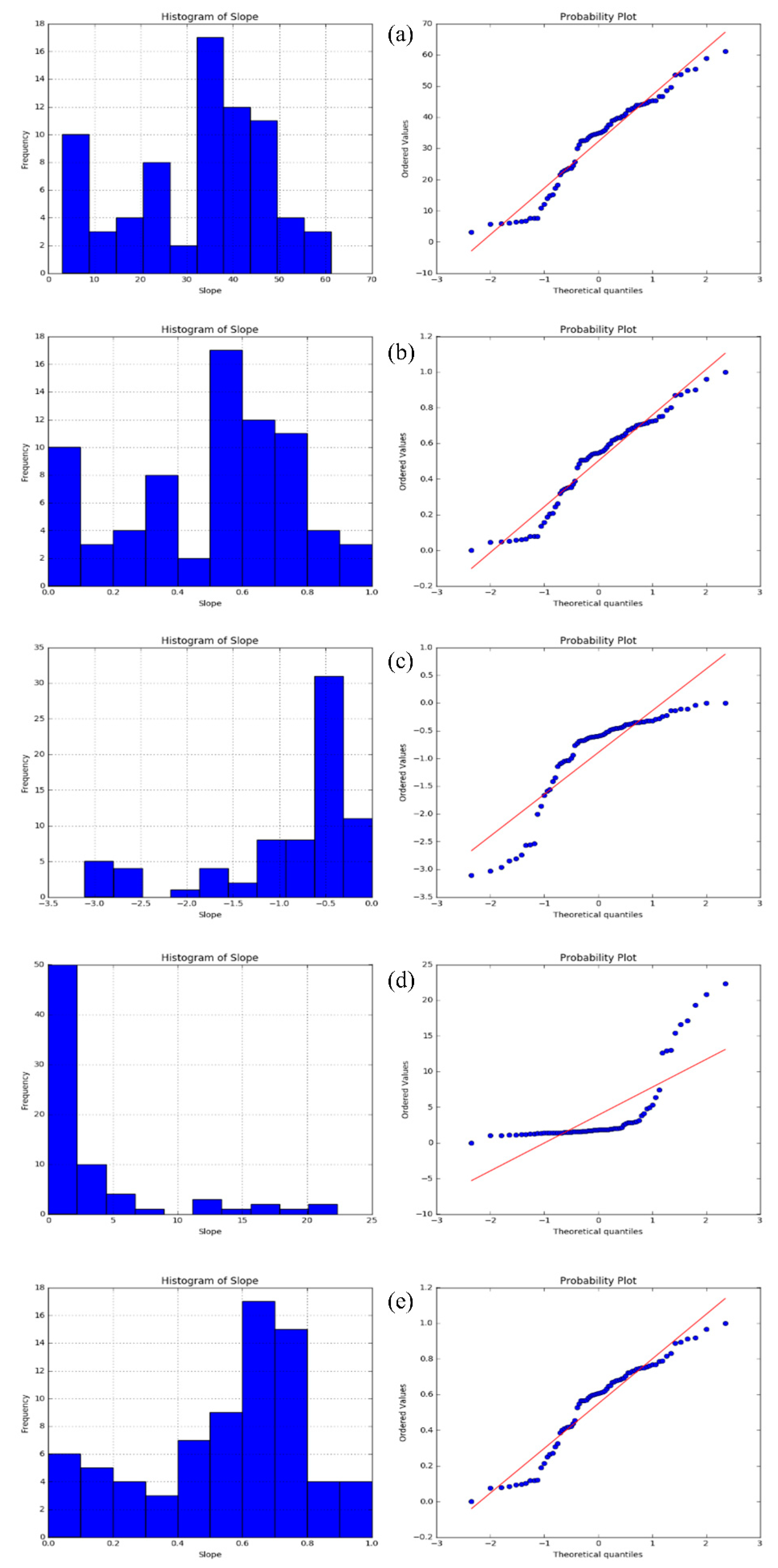
4.1. Descriptive Statistics of the Data

Each model might have a different and specific response to the variables and their transformation forms. Feature or variable transformations have the potential to enhance the training and performance of ML models, yet, it is not clear how these transformations affect the landslide modeling.
Initially, several extracted statistics from the continuous variables are needed to apply the transformation functions to different models. To this end, some common statistics such as mean, standard deviation, minimum, 25%, 50%, and 75% of probability, and maximum values of the conditioning factors (continuous variables) were generated. Table 2 shows the corresponding statistics for each continuous conditioning factor. These statistics were then applied to the transformation functions to generate transformed forms of the variables.
The significance of each factor (e.g., slope) in landslide occurrence varies with the other factors [2,45]. In many cases, the slope of prone areas is an essential part of landslide occurrence. Several studies on the same study area also suggested that the slope was the most dominant factor, and areas with a slope greater than 25 degrees are exceedingly prone to landslides [2,7]. To this end, slope variables derived from DEM were transformed into various forms of functions, namely Std-X, Log-X, Rec-X, and Power-X, and then were compared with the original slope values. Histograms and the Q-Q plots were employed to visualize the pattern and behavior of the samples after the transformations (Figure 5).
The Q-Q plot was used as a graphical tool, as it can evaluate a set of data plausibly following some theoretical distribution (e.g., normal or logarithmic). If an ML algorithm is run that assumes the dependent variables are normally distributed, the normal Q-Q plot can then be used to investigate that assumption. The Q-Q plots can be formed for any kind of variable distribution. It can be interpreted by plotting two sets of quantiles against each other. If both sets of quantiles came from the same distribution form, they should create a straight line. Figure 5a shows the histogram and the Q-Q plots of the original slope values (base case) of the current study. This base case acts as a benchmark for comparison with other transformation forms (Figure 5b–e).
The Q-Q plot of the base statues (Figure 5a) shows that variables roughly revolve around the straight line. This result indicates that the variables are practically close to the normal distribution; the corresponding histogram also confirms this form of data distribution. When the Std-X was applied to the data, the samples were normalized in a range from 0 to 1, and the Q-Q plot remained unchanged. This finding suggests that the data were similar to the normal form (Figure 5b), whereas employing the Log-X (Figure 5c), shows the points in the plot seem to fall about a straight line but are more distanced. The corresponding histogram also reflects the same ranging from −2 to 0. The Log-X could provide a better understanding of models that have an equal or close distribution with the logarithmic function. Using the Rec-X plot (Figure 5d), the points fall along a line in the middle of the graph but curve off in the extremities. This behavior generally suggests that data have more extreme values than would be expected if they truly came from a normal distribution. When the Power-X were used (Figure 5e), the points seem to fall about a straight line and the histogram shows the values normalized by a range from 0 to 1. This could provide a condition for the model to take advantage of a better understanding of the learning process.

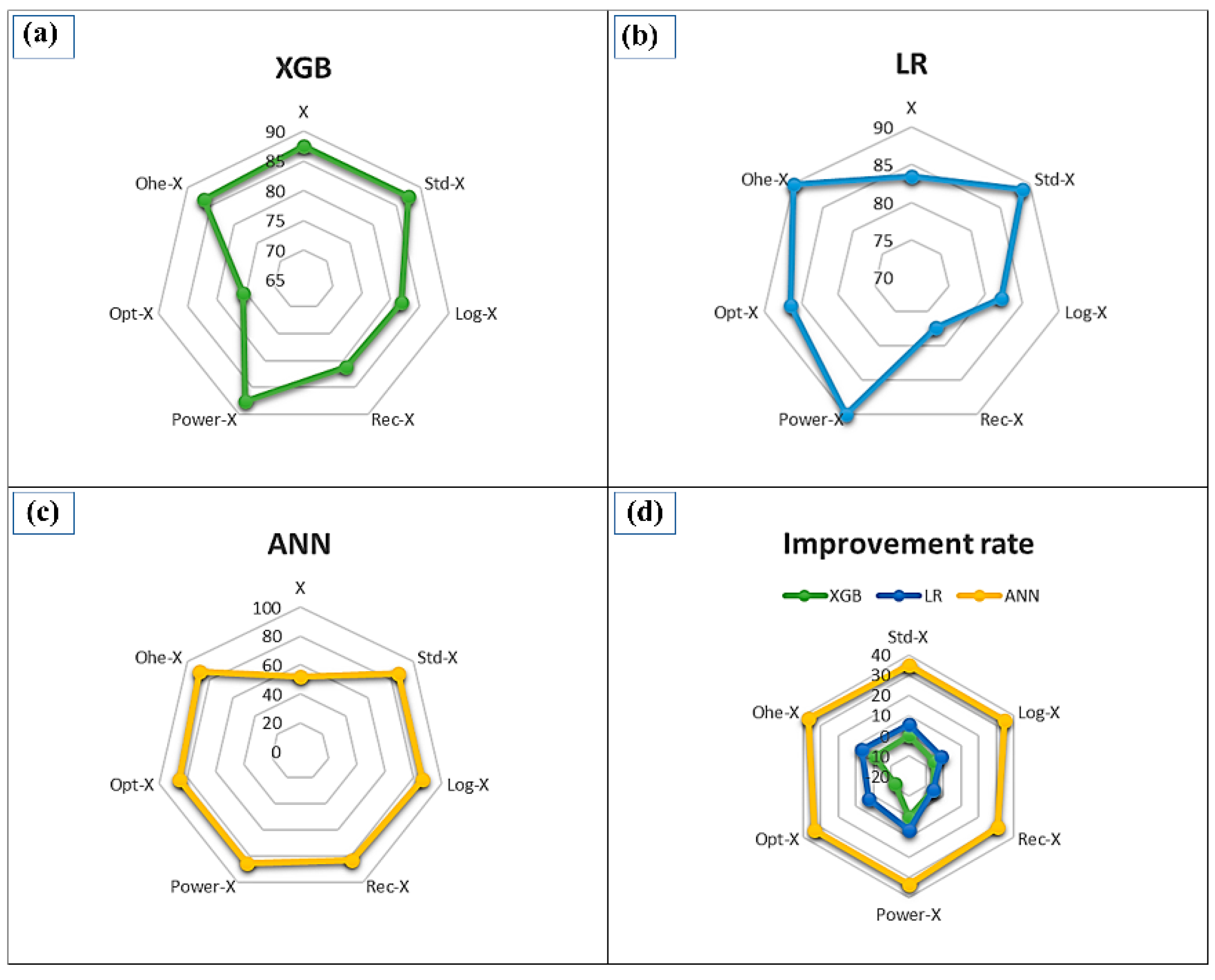
4.2. Impact of the Feature Transformations Applied to the Benchmark Models

The impact of six scenarios of feature transformations applied was compared with the base model (the default case often used in the landslide modeling). To this end, XGB, LR, and ANN were chosen from different ML families/groups as benchmark models for a fair comparison. The 10-fold cross-validation was selected due to its functional ability to better understand the training of samples and to avoid over/under prediction. Table 3 shows the comparative performance of the models with their corresponding transformation scenarios.

4.2.1. Impact of the Feature Transformations on XGB

XGB was executed using the XGBoost package in the R and the remaining parameters were used to the default value with Nrounds set to 10. The key parameters were selected as Subsample ratio of columns (colsample_bytree): 0.5; maximum tree depth (“max_depth”): 5; the proportion of data instances to grow tree (“subsample”): 0.7. The results from Table 3 show that using Power-X and Std-X, the performance stood unchanged by the accuracy of 87.546 whereas using the other remained transformations resulted in the performance of all models dramatically dropping (the worst performance was recorded as 75.427 using the Opt-X). This indicates that XGB has not received any advancement from the transformations; this is because XGB models are created in a way that predicts the residuals or errors of prior models and are then added together to make the final prediction. It also uses a gradient descent algorithm to minimize the loss when adding new models and it has proven to push the limits of computing speed. In general, XGB showed its tough resistance toward all feature transformations.

4.2.2. Impact of the Feature Transformations on LR

In LR, the landslide conditioning factors were first transformed into a logit variable. Following this, the maximum likelihoods were computed from the logit variables. When the Ohe-X functions were used, LR scored a comparable performance by the accuracy of 89.960. This result implies that LR worked better when the dependent variables were in a categorical/binary form. This privilege of LR provides a better condition to describe the data and to explain the relationship between one dependent binary variable and one or more nominal, ordinal, interval, or ratio-level independent variables. LR also had an efficient result in the base case with an accuracy of 83.434 and was useful in the Power-X condition with an accuracy of 89.983. We anticipated this as the variables in LR do not need to have a normal distribution.
Conversely, using the Rec-X function, the performance dropped to 77.365; this poor performance could happen as the classes are highly correlative or highly nonlinear, the coefficients of the model cannot correctly predict the gain/loss from each individual feature. Moreover, outliers and leverage points can sway the decision boundary, causing poor performance. In general, LR performance seems efficient because LR is easy and quick to implement, and simplifies the relationship between categorical data and certain dependent variables that can be categorical, continuous, or binary. In addition, it performs well when the dataset is linearly separable and less prone to over-fitting. The main limitation in LR is the assumption of linearity between the dependent variable and the independent variables.

4.2.3. Impact of the Feature Transformations on ANN

To establish the ANN model, the numbers of input, hidden, and output layers should be determined first. In this study, each of the input, hidden, and output layers consisted of a single layer. The activation function was set as a rectified linear unit (ReLU), the number of hidden layers was chosen as one, the number of hidden units in a hidden layer were 62 units and the learning rate was 0.01. Table 3 shows that, by engaging a diversity of feature transformations, the performance of ANN was remarkably improved. The ANN achieved the highest 10-fold cross-validation accuracy of 89.398 when the Ohe-x function was employed so that the improvement rate was raised by 37.154%. This implies that the model was able to better understand the learning scheme when the categorical features were employed. In contrast, ANN displays the worst performance of 52.244, when the base case (without transformation) was used. This indicates that ANN is highly dependent on the quality of the input data and its distribution forms. ANN received the most advantages from the transformations since these transformations could offer less complexity, providing more efficient training practice. Overall, ANN showed the highest accuracy in the feature transformations assessment.

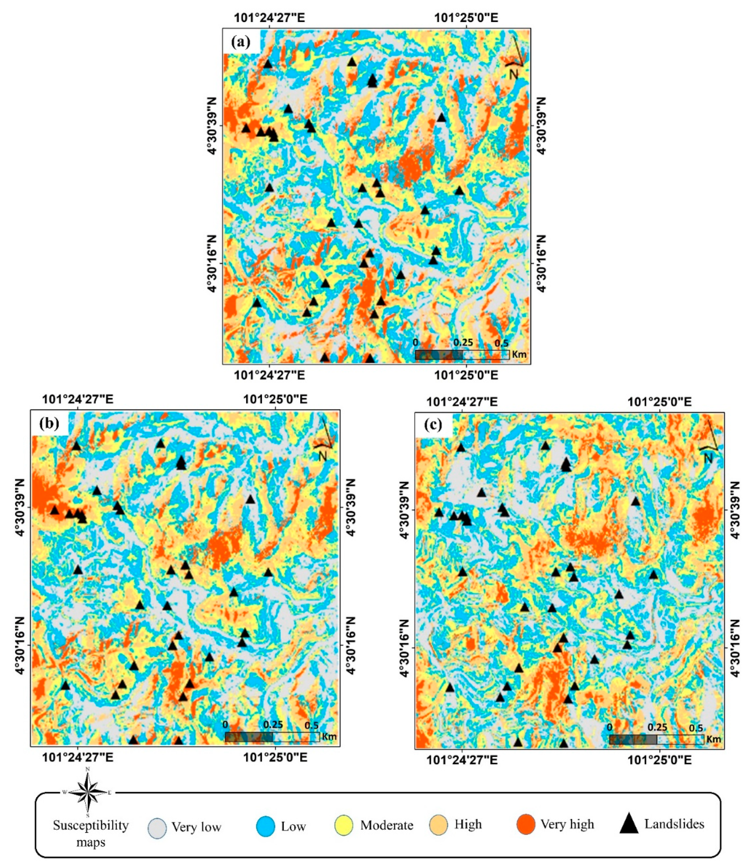
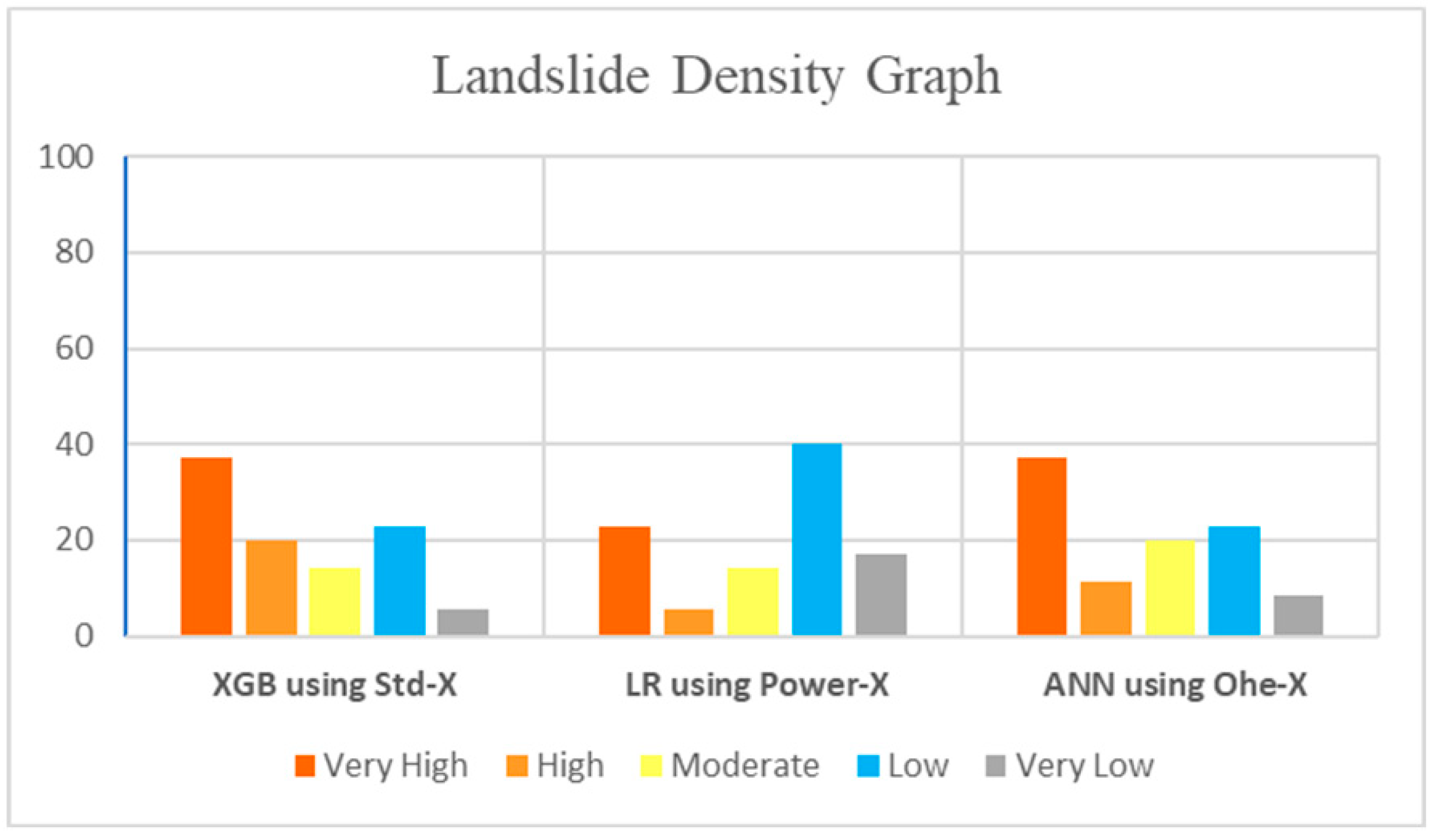
4.3. Landslide Susceptibility Maps

After assessing the models, the landslide susceptibility maps were generated based on the best result of each ML group (Figure 6). Five susceptible classes (i.e., very-low, low, moderate, high, and very-high) were categorized based on natural break classification carried out by ArcGIS software (Jenk’s method). Specifically, the values for each class were as follows: (very-low (<0.2), low (0.2–0.4), moderate (0.4–0.6), high (0.6–0.8), and very-high (>0.8). The natural break is a common method for preparing landslide susceptibility mapping and is designed to calculate the best value ranging in diverse classes [4]. This classification decreases the average deviation from the mean class’s value while increasing the deviation from the other classes’ mean. It is an iterative process that repeats the calculation in different breaks until it reaches the smallest variance in the class. From the visual interpretation, it can be observed that the ANN model showed comparable results with XGB and LR models. However, the overall performance of all models was relatively efficient (close to 90%).
The landslide susceptibility maps of the area were validated using the ROC curve (Figure 7). Furthermore, landslide density graphs were used to assess the validity of landslide susceptibility maps, showing the landslide percentage that occurred in landslide susceptibility classes [70]. The model evaluation determined by the density graph is shown in Figure 8.
The ROC curve was used to evaluate the predictive capability of the improved models (Figure 7). The curves demonstrated that the ANN model (using Ohe-X transformation) scored the highest ROC value of 0.932, followed by XGB (without transformation/Std-X), and LR (using Power-X) by values of 0.916 and 0.832, respectively. This quantitative assessment validated the significant improvement of ANN through transformations and less sensitivity of the XGB to transformations than LR and ANN.
Further model evaluation was carried out by generating landslide density graphs. According to the results in Figure 8, the number of landslides in each susceptibility class was calculated and plotted in a two-dimensional graph, where its horizontal axis exhibited the susceptibility class, and the number of landslides was shown on the vertical axis. The outcomes showed that the XGB using Std-X, and ANN using Ohe-X, models predicted the highest landslide ratio of (37.14%) in the very-high class. Additionally, the LR using the Power-X model predicted 23% of landslides in the very-high susceptibility class. The landslide density graph showed the robustness of these models in predicting landslide inventories at a very-high susceptible level.

5. Discussion

Due to the internal processes of ML methods, normalized input variables are often preferred for modeling as they provide a better practice for the training. That is why these models perform better when the distribution of input data is normal or normal-like. However, often the input data might not be normally distributed. This issue received less attention in most of the previous landslide susceptibility modeling, as in most cases, the default setting of ML was employed. Feature transformations, as pre-processing steps, are techniques that can deal with this problem and improve the training performance by transforming the input data into a more normal-like form [8]. This investigation can provide the required awareness and motivate landslide experts to pay more attention when building their robust models. For this purpose, we studied the influence of six feature transformation functions applied to three standard ML methods.
Earlier studies using the XGB, LR, and ANN methods led to several important findings. For a fair assessment, a cross-validation approach (that was carried out in the present study) is required/recommended for the selection of training samples by a random process [71,72]. Wang et al. [73] reported that the LR model outperformed the ANN model and that selecting appropriate landslide samples for training the models could improve the model’s accuracy. In their LR model, the higher percentage of landslide points concentrated in high and very-high classes (while in the current study, the performance of ANN was higher than LR using the benefit of Ohe-X transformation) [73]. In another work by Zhou et al. [66], the LR model showed a lower performance compared to the ANN model due to complex nonlinear problems (while in the current study, the LR outperformed the ANN when none of the transformations were used) [66]. Previous works also suggested optimizing the training dataset as well as the model parameters for better susceptibility modeling [72]. These ML models were widely implemented in landslide susceptibility assessments and were concluded to have promising predictive capabilities with certain limitations/challenges.
We studied the ML feature transformation methods for improving landslide modeling to further reduce the challenges that exist in landslide susceptibility. In this regard, if a model can learn its own model based on engineered features, there is no need to recreate the features to perform the best from the first step in the beginning. Therefore, most of the models are highly recommended to be fed by appropriately engineered data/variables. Figure 9 illustrates the benefits received from various transformation models applying to XGB (Figure 9a), LR (Figure 9b), and ANN (Figure 9c). Figure 8d visually depicts the percentage of the improvement rate of all models, indicating that the further the distance from the center, the more benefit a model receives from a particular transformation. The ANN received the most advantages from the feature engineering (Figure 9c,d) by an improvement rate of 37.154% when Ohe-X transformation was used, while the XGB demonstrated a solid resistance against all transformation models (Figure 9d). The lowest accuracy of XGB was recorded when Opt- X was used because only two categorical variables were involved in the transformation process (Figure 9a).
The LR worked relatively well in its base model, which could be an indication of the fact that the LR does not necessarily need a normal form of data distribution. This could be attributed to its nonparametric nature, which permits the model to perform with skewed distribution data, a phenomenon that can also be observed in the natural environment and landslide conditioning factors. Power-X (as the top performance) was able to increase the efficiency of the training, by providing a further normal-like condition to the data. The Rec-X had the worst impact on the LR because the model could not correctly predict the gain or loss from each individual feature due to highly nonlinear features (Figure 9b). Considering LR advantages, it requires a shorter processing time than ANN; moreover, it is fairly easy to implement, very efficient to train, and serves as a good option for starting the modeling as a benchmark and tries using more sophisticated algorithms from thereon. Nevertheless, it uses linear combinations of variables which is not proficient at modeling entirely complex nonlinear problematic.
Furthermore, the XGB recorded its maximum performance of 87.546, when no transformation was used (Figure 9a). This optimistic performance shows that XGB can learn to re-generate that feature with less error, which means that the model can learn the engineered feature with no additional support by transformers. This performance of XGB is due to the potential of performing three primary forms of gradient boosting (gradient boosting, stochastic boosting, and regularized boosting) and it is strong enough to maintain the fine-tuning and regularization factors. It is also speedy (parallel computation) and highly efficient due to its scalability. However, as a drawback, it only works with numeric features and could experience overfitting if hyperparameters are not adjusted appropriately. The current work suggests that careful pre-processing of the input data is required before the actual modeling. The outliers, highly correlated factors, and noisy data should be pre-processed to reduce the final training data selection product effects. Comparison of several models, the XGB model suggested a better option for accurate modeling because the knowledge domain is different from one area to another.
Overall, this study suggests that XGB can competently deal with the input variables/conditioning factors without using transformations. However, in the case of dealing with categorical variables, using the feature transformations seems more feasible and recommended. Regarding the continuous variables, using Std-X and Power-X are highly suggested. However, the one-hot encoding transformation is more valued when it comes to categorical condition factors.

6. Conclusions

The ML has been shown to be an effective landslide susceptibility mapping method in recent years. Diverse approaches have been made in the last few years, demonstrating the success of several algorithms to enhance landslide assessment, including different architectures, factor optimizations, and training/sampling practices. The effect of several pre-processing steps before the main landslide modeling, including normalization in the range of zero to one (such as minimax normalization), feature selection/elimination, multicollinearity analysis, and quality of training, were also investigated. Nevertheless, the impact of various feature transformations/engineering of the input data was not well studied. Most of the existing landslide modeling uses/assumes the normal distribution of input variables (default setting), which may not always be accurate. In this study, several feature transformation solutions were applied to three ML methods, such as XGB, LR, and ANN. The result suggested that the ANN model achieved the most significant advantages using the Ohe-X function by the advancement rate of 37.154%, reaching its best efficiency of 89.398. When the Power-X and Ohe-X functions were employed, the LR model showed an improvement rate of 6.5%. On the other hand, the XGB model achieved the best performance of 87.546 when the base model (without transformation) was used. The outcome of this research can help geoscientists and landslide experts to carefully consider the quality of input data before the primary modeling, as specific models might be considerably affected by certain types of transformation functions. By utilizing appropriate transformation strategies, further generalized state-of-the-art models can be formulated. While, in this paper, we carried out a comparative study on a small area, employing the model on a larger area would examine the robustness and transferability of the model. Moreover, the study could be replicated in other geographical set-ups with different geo-environmental factors and other types of landslides such as deep-seated landslides.

Author Contributions

Project administration: B.P.; Conceptualization: H.A.H.A.-N., B.P.; Methodology: H.A.H.A.-N., and M.I.S.; Modeling: H.A.H.A.-N., and M.I.S.; Writing original draft: H.A.H.A.-N. Supervision: B.P.; Validation: B.P.; Visualization: B.P.; Resources: B.P., and A.A.; Review and Editing: B.P., B.K., M.S., and A.A.; Funding acquisition: B.P., and A.A. All authors have read and agreed to the published version of the manuscript.

Funding

This research is funded by the Centre for Advanced Modelling and Geospatial Information Systems (CAMGIS), Faculty of Engineering and Information Technology, the University of Technology Sydney, Australia. This research was also supported by the Researchers Supporting Project number RSP-2021/14, King Saud University, Riyadh, Saudi Arabia.

Institutional Review Board Statement

Not applicable.

Informed Consent Statement

Not applicable.

Data Availability Statement

Raw data were generated at the University of Technology Sydney, Australia. Derived data supporting the findings of this study are available from the corresponding author [Biswajeet Pradhan] upon request.

Acknowledgments

The authors would like to thank the Faculty of Engineering and Information Technology, the University of Technology, Sydney, for providing all facilities during this research. We are also thankful to the Department of Mineral and Geosciences, the Department of Surveying, Malaysia, and the Federal Department of Town and Country Planning.

Conflicts of Interest

The authors declare no conflict of interest.

References

  1. Kavzoglu, T.; Colkesen, I.; Sahin, E.K. Machine learning techniques in landslide susceptibility mapping: A survey and a case study. Landslides Theory Pract. Model. 2018, 50, 283–301. [Google Scholar] [CrossRef]
  2. Pradhan, B.; Al-Najjar, H.A.H.; Sameen, M.I.; Mezaal, M.R.; Alamri, A.M. Landslide detection using a saliency feature enhancement technique from LIDAR-derived DEM and orthophotos. IEEE Access 2020, 8, 121942–121954. [Google Scholar] [CrossRef]
  3. Sameen, M.I.; Pradhan, B.; Bui, D.T.; Alamri, A.M. Systematic sample subdividing strategy for training landslide susceptibility models. CATENA 2019, 187, 104358. [Google Scholar] [CrossRef]
  4. Arabameri, A.; Pal, S.C.; Rezaie, F.; Chakrabortty, R.; Saha, A.; Blaschke, T.; Di Napoli, M.; Ghorbanzadeh, O.; Ngo, P.T.T. Decision tree based ensemble machine learning approaches for landslide susceptibility mapping. Geocarto Int. 2021, 2021, 1–35. [Google Scholar] [CrossRef]
  5. Napoli, M.D.; Martire, D.D.; Bausilio, G.; Calcaterra, D.; Confuorto, P.; Firpo, M.; Pepe, G.; Cevasco, A. Rainfall-induced shallow land-slide detachment, transit and runout susceptibility mapping by integrating machine learning techniques and GIS-based approaches. Water 2021, 13, 488. [Google Scholar] [CrossRef]
  6. Novellino, A.; Cesarano, M.; Cappelletti, P.; Di Martire, D.; Di Napoli, M.; Ramondini, M.; Sowter, A.; Calcaterra, D. Slow-moving landslide risk assessment combining Machine Learning and InSAR techniques. CATENA 2021, 203, 105317. [Google Scholar] [CrossRef]
  7. Pradhan, B.; Seeni, M.I.; Kalantar, B. Performance Evaluation and Sensitivity Analysis of Expert-Based, Statistical, Machine Learning, and Hybrid Models for Producing Landslide Susceptibility Maps. In Laser Scanning Applications in Landslide Assessment; Pradhan, B., Ed.; Springer: Cham, Switzerland, 2017. [Google Scholar] [CrossRef]
  8. Géron, A. Hands-On Machine Learning with Scikit-Learn, Keras, and TensorFlow: Concepts, Tools, and Techniques to Build. Intelligent Systems, 2nd ed.; O’Reilly Media: Sebastopol, CA, USA, 2019. [Google Scholar]
  9. Brownlee, J. Master Machine Learning Algorithms: Discover How They Work and Implemen Them from Scratch; Machine Learning Mastery: Vermont, Australia, 2016. [Google Scholar]
  10. Box, G.E.P.; Cox, D.R. An analysis of transformations. J. R. Stat. Soc. Ser. B 1964, 26, 211–243. [Google Scholar] [CrossRef]
  11. Bengio, Y.; Courville, A.; Vincent, P. Representation learning: A review and new perspectives. IEEE Trans. Pattern Anal. Mach. Intell. 2013, 35, 1798–1828. [Google Scholar] [CrossRef]
  12. Coates, A.; Ng, A.; Lee, H. An analysis of single-layer networks in unsupervised feature learning. In Proceedings of the 14th International Conference on Artificial Intelligence and Statistics, Ft. Lauderdale, FL, USA, 11–13 April 2011; pp. 215–223. [Google Scholar]
  13. Hinton, G.E.; Salakhutdinov, R.R. Reducing the dimensionality of data with neural networks. Science 2006, 313, 504–507. [Google Scholar] [CrossRef] [PubMed] [Green Version]
  14. Jolliffe, I.T. Principal component analysis for special types of data. Prin. Compon. Anal. 2002, 2002, 338–372. [Google Scholar]
  15. Olshausen, B.A.; Field, D.J. Emergence of simple-cell receptive field properties by learning a sparse code for natural images. Nature 1996, 381, 607–609. [Google Scholar] [CrossRef] [PubMed]
  16. Pechenizkiy, M.; Tsymbal, A.; Puuronen, S. PCA-based feature transformation for classification: Issues in medical diagnostics. In Proceedings of the 17th IEEE Symposium on Computer-Based Medical Systems, Bethesda, MD, USA, 25 June 2004. [Google Scholar] [CrossRef] [Green Version]
  17. Haixiang, G.; Yijing, L.; Shang, J.; Mingyun, G.; Yuanyue, H.; Bing, G. Learning from class-imbalanced data: Review of methods and applications. Expert Syst. Appl. 2017, 73, 220–239. [Google Scholar] [CrossRef]
  18. Kim, K.-J.; Lee, W.B. Stock market prediction using artificial neural networks with optimal feature transformation. Neural Comput. Appl. 2004, 13, 255–260. [Google Scholar] [CrossRef]
  19. Abe, M.; Aoki, K.; Ateniese, G.; Avanzi, R.; Beerliová, Z.; Billet, O. Lecture Notes in Computer Science (Including Subseries Lecture Notes in Artificial Intelligence and Lecture Notes in Bioinformatics); 3960 LNCS:VI; Springer: Berlin/Heidelberg, Germany, 2006. [Google Scholar]
  20. García, V.; Sánchez, J.; Mollineda, R. On the effectiveness of preprocessing methods when dealing with different levels of class imbalance. Knowl.-Based Syst. 2012, 25, 13–21. [Google Scholar] [CrossRef]
  21. Hussin, H.Y.; Zumpano, V.; Reichenbach, P.; Sterlacchini, S.; Micu, M.; van Westen, C.; Bălteanu, D. Different landslide sampling strategies in a grid-based bi-variate statistical susceptibility model. Geomorphology 2016, 253, 508–523. [Google Scholar] [CrossRef]
  22. Mezaal, M.R.; Pradhan, B.; Sameen, M.I.; Shafri, H.Z.M.; Yusoff, Z.M. Optimized neural architecture for automatic landslide detection from high-resolution airborne laser scanning data. Appl. Sci. 2017, 7, 730. [Google Scholar] [CrossRef] [Green Version]
  23. Merghadi, A.; Yunus, A.P.; Dou, J.; Whiteley, J.; ThaiPham, B.; Bui, D.T.; Avtar, R.; Abderrahmane, B. Machine learning methods for landslide susceptibility studies: A comparative overview of algorithm performance. Earth-Sci. Rev. 2020, 207, 103225. [Google Scholar] [CrossRef]
  24. Steger, S.; Brenning, A.; Bell, R.; Glade, T. Incompleteness matters-An approach to counteract inventory-based biases in statistical landslide susceptibility modelling. In EGU General Assembly Conference Abstracts; EGU: Vienna, Austria, 2018; p. 8551. [Google Scholar]
  25. Canoglu, M.C.; Aksoy, H.; Ercanoglu, M. Integrated approach for determining spatio-temporal variations in the hydrodynamic factors as a contributing parameter in landslide susceptibility assessments. Bull. Int. Assoc. Eng. Geol. 2018, 78, 3159–3174. [Google Scholar] [CrossRef]
  26. Samia, J.; Temme, A.; Bregt, A.K.; Wallinga, J.; Stuiver, J.; Guzzetti, F.; Ardizzone, F.; Rossi, M. Implementing landslide path dependency in landslide susceptibility modelling. Landslides 2018, 15, 2129–2144. [Google Scholar] [CrossRef] [Green Version]
  27. Hussin, H.; Zumpano, V.; Sterlacchini, S.; Reichenbach, P.; Bãlteanu, D.; Micu, M.; Bordogna, G.; Cugini, M. Comparing the predic-tive capability of landslide susceptibility models in three different study areas using the weights of evidence technique. In EGU General Assembly Conference Abstracts; EGU2013-12701; EGU: Vienna, Austria, 2013. [Google Scholar]
  28. Arnone, E.; Francipane, A.; Scarbaci, A.; Puglisi, C.; Noto, L. Effect of raster resolution and polygon-conversion algorithm on landslide susceptibility mapping. Environ. Model. Softw. 2016, 84, 467–481. [Google Scholar] [CrossRef]
  29. Mezaal, M.R.; Pradhan, B.; Rizeei, H.M. Improving landslide detection from airborne laser scanning data using optimized dempster–shafer. Remote. Sens. 2018, 10, 1029. [Google Scholar] [CrossRef] [Green Version]
  30. Pradhan, B. Laser Scanning Applications in Landslide Assessment; Springer: Berlin/Heidelberg, Germany, 2017. [Google Scholar] [CrossRef]
  31. Soma, A.S.; Kubota, T.; Mizuno, H. Optimization of causative factors using logistic regression and artificial neural network models for landslide susceptibility assessment in Ujung Loe Watershed, South Sulawesi Indonesia. J. Mt. Sci. 2019, 16, 383–401. [Google Scholar] [CrossRef]
  32. Feizizadeh, B.; Roodposhti, M.S.; Blaschke, T.; Aryal, J. Comparing GIS-based support vector machine kernel functions for landslide susceptibility mapping. Arab. J. Geosci. 2017, 10, 122. [Google Scholar] [CrossRef]
  33. Pradhan, B. A comparative study on the predictive ability of the decision tree, support vector machine and neuro-fuzzy models in landslide susceptibility mapping using GIS. Comput. Geosci. 2013, 51, 350–365. [Google Scholar] [CrossRef]
  34. Roy, A.C.; Islam, M. Predicting the Probability of Landslide using Artificial Neural Network. In Proceedings of the 5th International Conference on Advances in Electrical Engineering (ICAEE), Dhaka, Bangladesh, 26–28 September 2019; pp. 874–879. [Google Scholar] [CrossRef]
  35. Zhang, Y.; Ge, T.; Tian, W.; Liou, Y.A. Debris flow susceptibility mapping using machine-learning techniques in Shigatse area, China. Remote. Sens. 2019, 11, 2801. [Google Scholar] [CrossRef] [Green Version]
  36. Yousefi, S.; Pourghasemi, H.R.; Emami, S.N.; Pouyan, S.; Eskandari, S.; Tiefenbacher, J.P. A machine learning framework for multi-hazards modeling and mapping in a mountainous area. Sci. Rep. 2020, 10, 12144. [Google Scholar] [CrossRef] [PubMed]
  37. Nhu, V.-H.; Shirzadi, A.; Shahabi, H.; Singh, S.K.; Al-Ansari, N.; Clague, J.J.; Jaafari, A.; Chen, W.; Miraki, S.; Dou, J.; et al. Shallow landslide susceptibility mapping: A comparison between logistic model tree, logistic regression, naïve bayes tree, artificial neural network, and support vector machine algorithms. Int. J. Environ. Res. Public Health 2020, 17, 2749. [Google Scholar] [CrossRef] [PubMed]
  38. Schlögel, R.; Marchesini, I.; Alvioli, M.; Reichenbach, P.; Rossi, M.; Malet, J.-P. Optimizing landslide susceptibility zonation: Effects of DEM spatial resolution and slope unit delineation on logistic regression models. Geomorphology 2017, 301, 10–20. [Google Scholar] [CrossRef]
  39. Conoscenti, C.; Rotigliano, E.; Cama, M.; Arias, N.A.C.; Lombardo, L.; Agnesi, V. Exploring the effect of absence selection on landslide susceptibility models: A case study in Sicily, Italy. Geomorphology 2016, 261, 222–235. [Google Scholar] [CrossRef]
  40. Tsangaratos, P.; Ilia, I. Comparison of a logistic regression and Naïve Bayes classifier in landslide susceptibility assessments: The influence of models complexity and training dataset size. CATENA 2016, 145, 164–179. [Google Scholar] [CrossRef]
  41. Pradhan, B.; Lee, S. Landslide susceptibility assessment and factor effect analysis: Backpropagation artificial neural networks and their comparison with frequency ratio and bivariate logistic regression modelling. Environ. Model. Softw. 2010, 25, 747–759. [Google Scholar] [CrossRef]
  42. Pradhan, B.; Lee, S. Regional landslide susceptibility analysis using back-propagation neural network model at Cameron Highland, Malaysia. Landslides 2009, 7, 13–30. [Google Scholar] [CrossRef]
  43. Evans, J.S.; Hudak, A.T. A multiscale curvature algorithm for classifying discrete return LiDAR in forested environments. IEEE Trans. Geosci. Remote. Sens. 2007, 45, 1029–1038. [Google Scholar] [CrossRef]
  44. Jebur, M.N.; Pradhan, B.; Tehrany, M.S. Optimization of landslide conditioning factors using very high-resolution airborne laser scanning (LiDAR) data at catchment scale. Remote. Sens. Environ. 2014, 152, 150–165. [Google Scholar] [CrossRef]
  45. Al-Najjar, H.A.H.; Kalantar, B.; Pradhan, B.; Saeidi, V. Conditioning factor determination for mapping and prediction of landslide susceptibility using machine learning algorithms. In Proceedings of the Proceedings Volume 11156, Earth Resources and Environmental Remote Sensing/GIS Applications X, Strasbourg, France, 10–12 September 2019; p. 111560. [Google Scholar] [CrossRef]
  46. Wilson, J.P.; Gallant, J.C. Terrain Analysis: Principles and Applications; John Wiley & Sons: Hoboken, NJ, USA, 2000. [Google Scholar]
  47. Lee, S.; Ryu, J.-H.; Min, K.; Won, J.-S. Landslide susceptibility analysis using GIS and artificial neural network. Earth Surf. Process. Landforms 2003, 28, 1361–1376. [Google Scholar] [CrossRef]
  48. Zheng, A.; Casari, A. Feature Engineering for Machine Learning: Principles and Techniques for Data Scientists; O’Reilly Media, Inc.: Newton, CA, USA, 2018. [Google Scholar]
  49. Heaton, J. An empirical analysis of feature engineering for predictive modeling. In Proceedings of the SoutheastCon 2016, Norfolk, VA, USA, 30 March–3 April 2016; pp. 1–6. [Google Scholar] [CrossRef] [Green Version]
  50. Auer, T. Pre-Processing Data. 2019. Available online: https://scikit-learn.org/stable/modules/preprocessing.html#standardization-or-mean-removal-and-variance-scaling (accessed on 1 March 2021).
  51. Ray, S. A Comprehensive Guide to Data Exploration. 2016. Available online: https://www.analyticsvidhya.com/blog/2016/01/guide-data-exploration/ (accessed on 1 March 2021).
  52. sklearn.preprocessing.MinMaxScaler. 2020. Available online: https://scikit-learn.org/stable/modules/generated/sklearn.preprocessing.MinMaxScaler.html (accessed on 1 March 2021).
  53. Sarkar, D. Continuous Numeric Data. 2018. Available online: https://towardsdatascience.com/understanding-feature-engineering-part-1-continuous-numeric-data-da4e47099a7b (accessed on 15 December 2020).
  54. Calculus, F. Reciprocal Function. 2011. Available online: https://calculus.subwiki.org/wiki/Reciprocal_function (accessed on 10 April 2021).
  55. Power Functions. 2020. Available online: https://www.brightstorm.com/math/precalculus/polynomial-and-rational-functions/power-functions/ (accessed on 10 April 2021).
  56. Ronaghan, S. The Mathematics of Decision Trees, Random Forest and Feature Importance in Scikit-Learn and Spark. Towards Data Science. 2018. Available online: https://towardsdatascience.com/the-mathematics-of-decision-trees-random-forest-and-feature-importance-in-scikit-learn-and-spark-f2861df67e3 (accessed on 1 March 2021).
  57. Micheletti, N.; Foresti, L.; Robert, S.; Leuenberger, M.; Pedrazzini, A.; Jaboyedoff, M.; Kanevski, M. Machine learning feature selection methods for landslide susceptibility mapping. Math. Geosci. 2014, 46, 33–57. [Google Scholar] [CrossRef] [Green Version]
  58. Brownlee, J. Why One-Hot Encode Data in Machine Learning. Mach. Learn. Mastery 2017. Available online: https://machinelearningmastery.com/why-one-hot-encode-data-in-machine-learning/ (accessed on 1 March 2021).
  59. Chen, T.; Guestrin, C. Xgboost: A scalable tree boosting system. In Proceedings of the 22nd Acm Sigkdd International Conference on Knowledge Discovery and Data Mining, New York, NY, USA, 13–17 August 2016; pp. 785–794. [Google Scholar] [CrossRef] [Green Version]
  60. Dewancker, I.; McCourt, M.; Clark, S. Bayesian optimization for machine learning: A Practical Guidebook. arXiv 2016, arXiv:1612.04858. [Google Scholar]
  61. Sonobe, R.; Yamaya, Y.; Tani, H.; Wang, X.; Kobayashi, N.; Mochizuki, K.-I. Assessing the suitability of data from Sentinel-1A and 2A for crop classification. GIScience Remote. Sens. 2017, 54, 918–938. [Google Scholar] [CrossRef]
  62. Georganos, S.; Grippa, T.; VanHuysse, S.; Lennert, M.; Shimoni, M.; Kalogirou, S.; Wolff, E. Less is more: Optimizing classification performance through feature selection in a very-high-resolution remote sensing object-based urban application. GIScience Remote. Sens. 2017, 55, 221–242. [Google Scholar] [CrossRef]
  63. Liu, T.; Abd-Elrahman, A.; Morton, J.; Wilhelm, V.L. Comparing fully convolutional networks, random forest, support vector machine, and patch-based deep convolutional neural networks for object-based wetland mapping using images from small unmanned aircraft system. GIScience Remote. Sens. 2018, 55, 243–264. [Google Scholar] [CrossRef]
  64. Santos, L.D. GPU Accelerated Classifier Benchmarking for Wildfire Related Tasks. Ph.D. Thesis, NOVA University of Lisbon, Lisbon, Portugal, 2018. [Google Scholar]
  65. Mondini, A.C.; Chang, K.T.; Chiang, S.H.; Schlögel, R.; Notarnicola, C.; Saito, H. Automatic mapping of event landslides at basin scale in Taiwan using a Montecarlo approach and synthetic land cover fingerprints. Int. J. Appl. Earth Obs. Geoinf. 2017, 63, 112–121. [Google Scholar] [CrossRef]
  66. Zhou, C.; Yin, K.; Cao, Y.; Ahmed, B.; Li, Y.; Catani, F.; Pourghasemi, H.R. Landslide susceptibility modeling applying machine learning methods: A case study from Longju in the Three Gorges Reservoir area, China. Comput. Geosci. 2018, 112, 23–37. [Google Scholar] [CrossRef] [Green Version]
  67. Sharma, N.; Chakrabarti, A.; Balas, V.E. Data management, analytics and innovation. In Proceedings of the ICDMAI, Macao, China, 8–11 April 2019. [Google Scholar] [CrossRef]
  68. Lee, S.; Pradhan, B. Landslide hazard mapping at Selangor, Malaysia using frequency ratio and logistic regression models. Landslides 2006, 4, 33–41. [Google Scholar] [CrossRef]
  69. Berrar, D. Cross-validation. J. Math. Psychol. 2019, 1, 542–545. [Google Scholar] [CrossRef]
  70. Kalantar, B.; Pradhan, B.; Naghibi, S.A.; Motevalli, A.; Mansor, S. Assessment of the effects of training data selection on the land-slide susceptibility mapping: A comparison between support vector machine (SVM), logistic regression (LR) and artificial neural networks (ANN). Geomat. Nat. Hazards Risk 2018, 9, 49–69. [Google Scholar] [CrossRef]
  71. Huang, Y.; Zhao, L. Review on landslide susceptibility mapping using support vector machines. CATENA 2018, 165, 520–529. [Google Scholar] [CrossRef]
  72. Pham, B.T.; Bui, D.T.; Prakash, I.; Dholakia, M. Hybrid integration of multilayer perceptron neural networks and machine learning ensembles for landslide susceptibility assessment at Himalayan area (India) using GIS. CATENA 2017, 149, 52–63. [Google Scholar] [CrossRef]
  73. Wang, L.J.; Guo, M.; Sawada, K.; Lin, J.; Zhang, J. A comparative study of landslide susceptibility maps using logistic regression, frequency ratio, decision tree, weights of evidence and artificial neural network. Geosci. J. 2016, 20, 117–136. [Google Scholar] [CrossRef]
Figure 1. Location of the study area: (a) map of Malaysia; (b) map of Cameron Highlands, and (c) the study area including landslide inventories.
Remotesensing 13 03281 g001
Figure 2. Landslide conditioning factors used in this study: (a) altitude; (b) slope; (c) aspect; (d) curvature; (e) distance to road; (f) distance to lineament; (g) distance to stream; (h) land use land cover; (i) TRI; (j) NDVI, and (k) vegetation density.
Remotesensing 13 03281 g002aRemotesensing 13 03281 g002b
Figure 3. Overall flowchart of the current study.
Remotesensing 13 03281 g003
Figure 4. The architecture of a feed-forward neural network.
Remotesensing 13 03281 g004
Figure 5. The histogram and the Q-Q plots of the slope values: (a) original slope values; (b) Std-X; (c) Log-X; (d) Rec-X, and (e) Power-X.
Remotesensing 13 03281 g005
Figure 6. Landslide susceptibility maps: (a) XGB using Std-X; (b) LR using Power-X, and (c) ANN using Ohe-X.
Remotesensing 13 03281 g006
Figure 7. The ROC values of the three models: (a) XGB using Std-X; (b) LR using Power-X, and (c) ANN using Ohe-X.
Remotesensing 13 03281 g007
Figure 8. Landslide density graph of the models for XGB using Std-X, LR using Power-X, and ANN using Ohe-X.
Remotesensing 13 03281 g008
Figure 9. The quantity of the advantages acquired by various transformation models: (a) XGB; (b) LR, and (c) ANN. (d) Percentage of improvement rate from the base model (The distance from the center indicates quantity of benefit received from the transformations).
Remotesensing 13 03281 g009
Table 1. Transformation approaches and functions used in the current study.
Transformation ApproachFunctionDescription
Minimax normalization (Std-X) y   = ( x m i n ) / ( m a x m i n ) When x = m i n , y is equal to 0 , whereas when x = m a x , the value of y is equal to 1 . This implies that the total range of X varied in a range from 0 to 1 [52].
Logarithmic functions (Log-X) y   =   log   a x Logarithmic functions are the inverses of exponential functions. The reverse of the exponential function y = a x is x = a y [53].
Reciprocal function
(Rec-X)
f ( x ) = 1 / x The reciprocal function is a function characterized by the set of nonzero real numbers, which sends every real number to its reciprocal value [54].
Power functions
(Power-X)
y   = x ^ ( 1 / 1.2 ) ) All power functions pass through the point (1,1) on the coordinate plane. It is a function where, y   =   x n A = π r 2 n so that n is any real constant number [55].
Optimal features selected by random forest
(Opt-X)
R F f i i = j n o r m f i i j j ϵ a l l f e a t u r e s , k ϵ a l l t r e e s n o r m f i j k Random forests are comprised of from 4 to 12 hundred choices of trees. Each tree has an additional order of Yes/No inquiries dependent on a singular or mixture of features. The importance of each feature is extracted from how “pure” every lot is [56,57].
One-hot encoding (Ohe-X) applied to land use and vegetation densityLand use and vegetation density encodingFor categorical variables, no ordinal relationship exists, and the integer encoding is not sufficient. One-hot encoding is applied to the integer representations. This is the place the integer encoded variable is unconcerned and another paired variable is added for every unique integer number [58].
Table 2. Summary statistics of the data used in the current study. The samples include a total of 70 events including 35 landslides (positive) and 35 random non-landslides (negative).
ItemSlopeCurvatureAspectDistance to
Lineament
Distance to
Road
Distance to StreamAltitudeTRI
mean32.16−1.05180.18108.4374.1937.921581.6549.53
std14.9619.61107.9375.3780.2827.7376.8614.64
min3.08−83.544.311.412.240.001466.2817.17
25%22.59−12.2887.7251.2417.5613.971520.7442.97
50%34.89−0.88175.7489.2248.5231.961574.0253.12
75%43.146.97281.97150.93100.1656.191620.1958.46
max61.1447.95359.57298.65343.42107.011795.6088.25
Table 3. Result of 10-cross-validation accuracy for XGB, LR, and ANN models by implementing different feature transformation techniques.
ModelAccuraciesPercentage of Improvement from the Base Model
XGBLRANNXGBLRANN
X87.54683.43452.244---
Std-X87.54688.76086.8070.0005.32634.563
Log-X81.88082.12586.974−5.666−1.30934.730
Rec-X81.28277.36582.888−6.264−6.06930.644
Power-X87.54689.98385.7080.0006.54933.464
Opt-X75.42786.41186.101−12.1192.97733.857
Ohe-X86.54489.96089.398−1.0026.52637.154
Publisher’s Note: MDPI stays neutral with regard to jurisdictional claims in published maps and institutional affiliations.

