1. Introduction
Studies aimed at analyzing the evolution of the high and rocky coasts are less numerous than those dedicated to the low and sandy coasts because of their greater economic interest. However, the high and rocky coasts are the main type of Italian coast [
1]. In recent decades, many rocky coastal areas of the Mediterranean coast have been affected by frequent and very intense geomorphological events. These include the phenomenon of erosion, which is increasing due to climate changes. In some Italian rocky coasts such as those of the Abruzzo region, the phenomenon is producing a significant increase in danger and risk for settlements, infrastructure, and residential and tourist buildings [
2]. This high level of risk was related both to anthropogenic factors (cut-slopes and deforestation) on the upslope and to an accelerated upslope cliff retreat due to the sea-level rise, increased winter rainfall, and more intense storm activity [
3].
Therefore, in order to identify more effective integrated strategies to preserve the coastlands and to prevent damage to human heritage, extensive modern geomorphological studies, based on detailed field surveys, multi-temporal aero-photogrammetric analyses, digital geomorphological maps, and qualitative geomorphological modelling, are carried out by the experts [
2,
4]. All these studies, cited in the overview by Guzzetti et al. [
5], are in some cases supported by engineering numerical stability analysis. If the expert-based geomorphological map, which is based on the operator’s implicit terrain-related knowledge of the area being studied [
6], requires skills derived from long training and experience [
7], this expert-based approach is subjective and it is difficult to carry out comparative analyses among land maps produced by different expert analysts or even by the same analyst in different places and times [
8]. Moreover, the interpretation and mapping of land components are extremely time consuming, difficult, and expensive tasks [
9].
In order to be effective, geomorphological analysis requires the prior creation of a numerical contour map, derived from a Digital Elevation Model (DEM), which describes in details and reliably the trend of the ground surface to be analyzed. From the point of view of data acquisition, in the case of areas of limited extension (tens of hectares) and with suitable sun exposure, the survey can be effectively carried out by means of Terrestrial Laser Scanner (TLS) that allows both high detail and high accuracy [
10,
11,
12,
13,
14]. For wide areas, the TLS technique is very demanding in terms of time and costs both for the operations of measurement on the ground and for data processing. Alternatively, it may be more appropriate to use the Aerial Laser Scanner (ALS) from a helicopter or aircraft [
15,
16,
17,
18]. The data acquired by lidar (Light Detection and Ranging) technique in terms of point cloud that are interpolated to build the DEM are very versatile as they can be used for various applications (landslides, basins, and roads). It is becoming increasingly common for local authorities to commission topographical surveys, also carried out periodically, on the territory for which they are competent. This provides scientists with the availability of updated and free of charge data [
19].
In addition to lidar surveying technique, a number of satellite sensors (Ikonos, Pleiades, Quickbird, Worldview, etc.) provide images at high metric and radiometric resolutions as well as short revisit times [
12,
20,
21,
22]. A stereo pair of commercial High-Resolution Satellite Images (HRSI) with metric resolution up to 0.30 m ground sampling distance (GSD) can be expensive but covers large areas of the order of 100 km
2, which are often sufficient for the study of landslide complexes [
23,
24].
Morphometric studies are essentially based on DEM derived maps that describe the basic components of the geographical features, such as elevation, slope, and aspect [
9,
25]. Booth et al. [
26] demonstrated that the slope distribution can reflect the interaction between geomorphic processes occurring in the same area. Previous studies have shown that individual earthflows often have similar topographic gradients to the surrounding terrain, suggesting that earthflows have shaped a large fraction of the surrounding landscape [
27], whereas Iwahashi et al. [
28] think that curvature and roughness are both important in describing landform surfaces.
In some cases, for a more complete analysis of the landform unit spatial derivative, other indicators are useful for identifying and quantifying hydrological and geomorphological processes, such as the topographic wetness index [
29], the stream power index [
30], and the aggradation and degradation index [
31]. Geological, geotechnical, and engineering approaches usually focus on studies on natural slope stability, hazard assessment, and landslide risk mitigation, considering only the landslide as a target object of interest and its short-term evolution. On the other hand, the engineering geomorphological approach considers both landslides and their spatial and temporal contexts, including sudden changes in control factors and determinants [
4].
The availability of DEM and feature maps derived from it has allowed the elaboration of digital object-oriented geomorphological maps. These geomorphological objects can be represented following a hierarchical and multiscale procedure according to precise ontological rules [
32]. Nevertheless, this objective map not only is less affected by human error but also can be used to objectively and quantitatively compare terrain units [
33,
34] and to allow us to obtain numerical descriptions of the topographic forms of the Earth at different spatiotemporal scales. For this purpose, engineering geomorphology uses different approaches, methods, and techniques, including classification of morphometric parameters, filtering techniques, cluster analysis, and multivariate statistics [
9,
25,
35,
36,
37].
However, although maps are widely used as a basis for these analyses, no particular attention is paid to their actual suitability as a support to geomorphological maps and physical modelling as well as to their accuracy. The lack of these requirements can lead to confusing possible errors in the maps with real geomorphological signals. It should be clear that the quality of the product obtained with these techniques depends on the correctness and precision of the data processing, so it is mandatory to develop a careful procedure for the elaboration of raw measures, focused on this particular application.
In this respect, we have been working on how to optimize the process of elaboration of multisource and multi-temporal remote sensing data to obtain DEM and derived feature maps. Our paper aims to underline the importance of having an accurate topographic base map, essential for a correct geomorphological spatiotemporal interpretation. This is particularly useful for hazard assessment and risk mitigation actions in areas in which morphology is rapidly evolving, such as the study area. In this perspective, the work aims to address the issue using an interdisciplinary approach that uses topographic and geomorphometric methods to correctly perform a detailed geomorphological digital mapping following the Salerno Method described in Dramis et al. [
32].
The results of this integrated and interdisciplinary analysis carried out on base maps derived from different sources and referred to different times allow to discriminate processing errors from the actual spatial and temporal variations of the topographic surface.
These maps have been useful to characterize, from a geomorphometric point of view, some contiguous areas that have been gradually modified because of morphodynamic activity due to active geomorphic processes, coastally, hilly, and gravitationally recognizable as a residue of a Pleistocene evolution. In this perspective, geomorphometric analyses are considered not only as a quantification of the spatial expression of a specific landscape but also as its progressive changes over time.
In the case study, a traditional, landslide-centric approach was previously used, focused on surface investigation, boreholes, and geotechnical monitoring [
38]. Less attention has been paid to the adjacent coastal slope, where there are tourist beaches and waterways also affected by active and retrogressive shallow and deep-seated landslides.
The goodness of the achieved result is tested through the expert-based geomorphological analysis of the area performed with the criteria indicated above, comparing the results of the geomorphometric analysis on three adjacent coastal sectors. Two survey techniques have been used and compared: ALS (archive data covering the Campania Region, Italy) and photogrammetry from stereo pairs of HRSI (Pleiades images). Particular attention is paid to the transition from Digital Surface Model (DSM) to Digital Terrain Model (DTM) by applying and comparing filtering methods. Once the DTM has been obtained, the residuals between the points of the cloud and the interpolated filtered surface are identified and analyzed using the cross-validation procedure. The distribution that better fits the histograms of frequency of the residuals is that of Laplace; potential outliers are identified and studied. Starting from the DTM obtained, a few geomorphological features are extracted.
2. Case Study Analysis
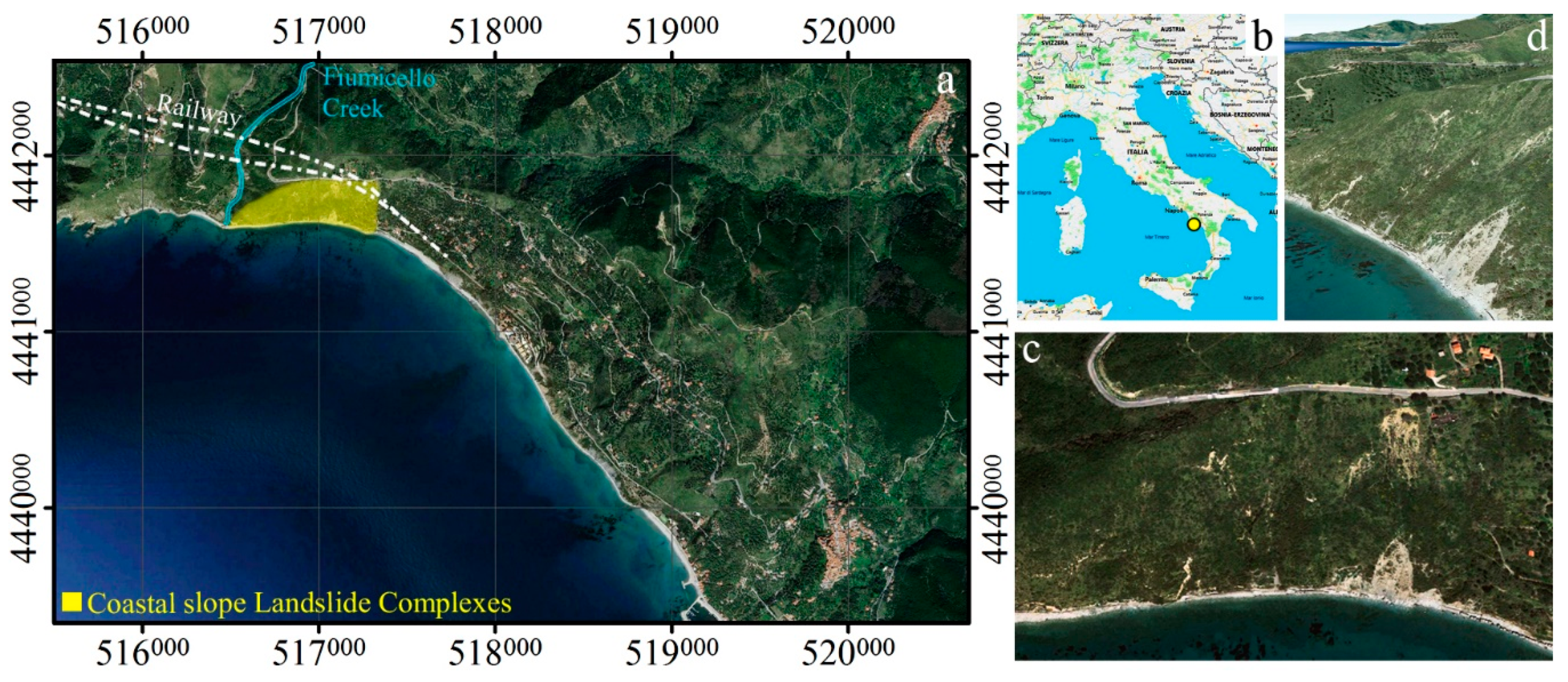
The study area is located in the municipality of Pisciotta along the Cilento coast of the Campania Region (Southern Italy), from the mouth of the Fiumicello creek to the Pisciotta Marina village harbor (
Figure 1). This coastal area is located on the south side of a hill, and has already been studied by the authors [
12,
38,
39], because it has been affected by a landslide system that has caused huge damage to the main road ‘Palinuro’ and the two sections of the railway line that connects Italy from north to south.
Given the importance of the integrity and functionality of the main railway lines, significant works for risk mitigation are being made at the toe of the landslide system along the stream (
Figure 1a). Less attention has been paid to the adjacent coastal slope, where there are beaches and water pipelines affected by active and retrogressive both shallow and deep-seated landslides (
Figure 1c,d). More recently, unpublished field surveys carried out by the authors and ongoing analyses on remote sensing images show both an enlargement toward southern of the landslide system flank and a retrogressive evolution by gravity-driven movements on the head coastal slope (
Figure 1c). Considering a paroxysmal evolution of two gravity-driven accelerated processes, a dramatic scenario characterized by a general collapse of both the slopes involving the railway line and all the valley-coastal systems is not to be excluded.
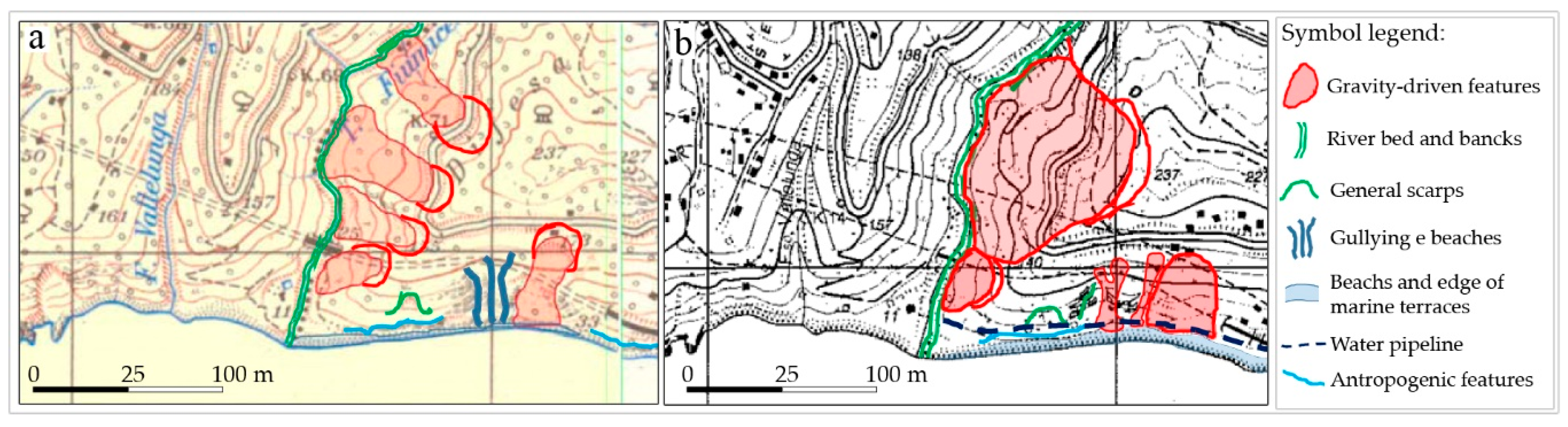
From a geomorphological point of view, previous research has identified many coastal slopes similar to the studied one as a typical “slope-over-wall” model [
1], composed of a convex, colluvial, debris upper slope laying on remnants of a buried, uplifted marine platform covered by rounded, gravelly marine deposits hanging on the cliffed bedrock toe slope (
Figure 2). The original, longer convex–concave profile was connected to a lower sea level (about 130 m below present-day sea level) during the last ice age. The cliffed toe slope has been progressively modeled by both the pure cliff retreat and the successive replacement and, finally, by the mechanisms of decline due to the postglacial rise in sea level up to present time. A threshold geomorphic behavior of the entire profile of the coastal slopes occurs after the complete breakage of the buried marine platform, with an intermediate gullying and channelized rapid earthflow stage and a subsequent general collapse due to gravity. By reinterpreting the above geomorphological evolution model in terms of spatiotemporal geomorphological zoning, three coastal sectors can be recognized and delimited, as shown in
Figure 2. This model will be used as a reference for the subsequent engineering geomorphological analyses performed on the topographic base maps.
3. Materials
In order to carry out a detailed geomorphometric analysis focused on distinguishing the topographical changes that affect the forms caused by processes that are no longer active from those resulting from ongoing processes or potentially triggering, it is necessary to do an archive research to find both technical documentation and survey campaigns in situ. In the literature, there are several geological and geomorphological studies on that stretch of coast, but there are no specific studies on the morphodynamics of that area. Consequently, we have analyzed the multi-temporal aerial photos, orthophotos, and topographic maps available on that area. Finally, high-resolution optical satellite images were analyzed and geo-referenced by Global Navigation Satellite System (GNSS) surveys. Another important source of metric data comes from a lidar survey.
3.1. Archive Data: Topographic Maps, Aerial Photos and Images
In order to reconstruct the relevant multi-temporal changes in topography, morphology, and land use, a number of aerial photographs have been analyzed, starting from the historical one taken in 1943 by the U.S. Army (
Figure 3a) up to the most recent orthophotos and Google Earth© images dating back to 2017 (
Figure 3b–f). On the images, significant morphological changes due to geomorphic processes are progressively highlighted in red. All the topographic maps available at the national level, relating to different period of survey, have been found and analyzed for multi-temporal environmental reconstruction. The first source of data is the 1:25,000 scale cartography from the IGM (Istituto Geografico Militare) archives, from the oldest published in 1956 to the recent 1994 edition (
Figure 4a,b). As in
Figure 3, significant morphological changes and other features due to geomorphic processes have also been highlighted on the topographic maps.
The analysis of the topographic maps shows, both for the hills inside the valley and for the coastal hillslopes, a medium-term geomorphic dynamic by gravity-driven, erosional, marine processes. Many of these processes affect anthropogenic features (roads, aqueducts, buildings, and managed tourist beaches), causing permanent damage and risks to life and the transport system as well as economic losses for the local population.
3.2. Lidar Data
The multitemporal analysis, in time steps, was also made using the images available on the National Cartographic Portal of the Italian Ministry of the Environment. The DEM obtained from a 2012 lidar survey was downloaded from the portal. The lidar data used are part of the database of the National Geoportal within the project Not-ordinary Plan of Environmental Remote Sensing of the Ministry of Environment and Protection of Land and Sea. As part of the project, aimed at verifying and monitoring areas of high hydrogeological risk, lidar flights were carried out over the river poles of the main network and the coastal strip. The characteristics of the data, declared by the authority that distributes the data, are as follows: density of points greater than 1.5 points per square meter, planimetric accuracy (2σ) of 30 cm, and altimetric accuracy (1σ) of 15 cm. The point clouds provided are already georeferenced in the UTM/ETRF00 system.
3.3. HRSI Data
The satellite images acquired belong to Pleiades-HR (High-Resolution Optical Imaging Constellation of centre national d’études spatiales—CNES). They have a nadir GSD of 0.5 m and a radiometric resolution of 11 bits. They were acquired in stereo mode on September 14, 2015 at 14:36 Greenwich Mean Time (GMT). Some characteristics of the stereo pair used are listed in
Table 1.
For georeferencing of the images and to obtain the stereo model, we used the software package Socet GXP ver. 4.2.0 by Bae Systems [
40], which implements a rigorous model of the sensor. The Ground Control Points (GCPs) were surveyed using GNSS receivers in nRTK (Network Real Time Kinematic) mode. To obtain a homogeneous distribution of GCPs, we designed a network in which the vertices are close to the nodes of a regular 2D grid. Thanks to the high speed of the NRTK surveys, we were able to measure more than one point near the nodes of the grid, so that we can choose among these points that are both better collimable on the image and characterized by the best measurement accuracy. We measured 70 GCPs, in our case, they are points which correspond to details of the ground or artefacts, 39 of which were used for image georeferencing. The reference system used is the ETRF00 with ellipsoidal heights.
To build the DEM, starting from the matching algorithms implemented in Socet GXP, we used the algorithm ASM (Automatic spatial modeler) recommended to extract dense clouds of 3D points from stereo images in highly vegetated areas at different heights [
40]. This software allows to have in output a file containing the coordinates of the matched points instead of those interpolated on a grid, allowing the operator to choose the interpolation algorithm to build the DEM at a later time with different software. To provide an indicator of the success of image digital matching, the software provides a numerical value, called figure of merit (FOM), ranging from 0 to 99, which is an index of correlation between homologous points. In the dark and shaded areas of the image, the FOM value obtained is obviously bad, it falls in the range 20–40. It is good practice to keep only the points with a FOM value higher than 40. Autocorrelated points with an FOM value under 40 have not been used to build the DEM.
Figure 5a shows one of the two stereo images with the distribution of the GCPs (small red circles) superimposed.
Figure 5b,c shows respectively the computed FOM values over the entire image and a zoom on a small area, including the landslide. The residuals of the georeferencing in the east (E), north (N), and height (h) are shown in
Figure 5d.
The values of the standard deviations of the residuals of the georeferencing of the images are rather low: σ
E = 5 cm, σ
N = 4 cm, and σ
h = 1 cm. However, they are not representative of the accuracy achieved. More significant is the standard deviations associated with the residuals computed on a number of Check Points (CPs), about 35 uniformly distributed over the surface. The average residue value and the associated standard deviations (σ
E = 18 cm, σ
N = 11cm, and σ
h = 47 cm) are shown in the box in
Figure 6.
Both the Pleiades and lidar point clouds have been aligned using the iterative closest point (ICP) algorithm, using the Pleiades point cloud as a reference. For the alignment, we used a much larger area than the one under study to include areas not subject to landslide movements and are therefore stable over time and common to both data sets.
4. Methods
To perform effective geomorphometric analysis and to produce digital geomorphological maps and geomorphic evolution models, engineering geomorphology needs very detailed contour maps and feature maps derived from high-resolution, high-accuracy numerical models. In some cases, input data are raw point clouds acquired by remote sensing techniques with very different characteristics and resolution. In general, to pass from the original point cloud to the numerical model (DEM), it must be filtered to remove all objects (vegetation, artifacts, etc.) that do not belong to the bare ground and then interpolated on the grid.
Both processes (filtering and interpolation) must be tested, and the accuracy of the result must be verified. In our case, it must also be taken into account that the data used are acquired at different times and, in that period, the topographic surface has changed because of the geomorphic processes ongoing. An analysis of the outliers made from an interdisciplinary point of view allows to identify some topographic singularities that are otherwise not identifiable and that are significant for the modeling and production of microscale geomorphological maps.
The following subsections describe the techniques used for filtering the raw data from lidar and Pleiades for the production of DEMs and for the evaluation of accuracy and modelling-oriented geomorphometric analysis.
4.1. Filtering of Lidar and Pleiades Data
The point clouds from lidar and photogrammetry are made of three components: bare ground, aboveground objects, and noise. Ground filtering should be able to isolate the points belonging to the ground from all the others in the cloud and to model the ground surfaces based on physical characteristics [
41]. The choice of the most effective filtering algorithm is not trivial. Three different filtering methods have been tested, with the aim of choosing the most suitable algorithm for the characteristics of our data: “GroundFilter”, implemented in the open source software FUSION; “LasGround” implemented in LAStools, a powerful library of scripts for ALS processing; and the Multiscale Curvature Classification (MCC) algorithm by Evans and Hudak [
42], implemented in MCC–lidar, a command-line tool for processing lidar data.
FUSION v. 3.30 software was developed by Forest Service of the U.S. Department of Agriculture (USDA). The “GroundFilter” command used to generate a surface corresponding to the bare ground belongs to the category of so-called interpolation-based filters. It has been adapted by Kraus and Pfeifer [
43] and is based on a linear prediction [
44].
It is an iterative process; in the first iteration, all points have equal weight and an average surface model is computed, so as to compute the residuals of the points with respect to the generated surface. Points above the generated surface will have less influence (less weight) than points below. Weights are used to generate the new surface in subsequent iterations. The number of iterations i can be set by the user (default i = 4). To create a ground surface, a few initial parameters must be provided such as the cell size and switches like the values of the g, w, a, and b parameters; tolerance for the final filtering; etc. The parameters a and b determine the slope of the weight function. The shift value g determines which points are assigned a weight of 1.0 (the maximum weight value). The ground offset parameter w is used to establish an upper limit for points to have an influence on the intermediate surface. Points above the level defined by (g + w) are assigned a weight equal to zero.
LAStools, a software suite by rapidlasso GmbH Company, is a collection of batch-scriptable, multicore command line tools. The tool used for the bare-earth extraction (LasGround) implements the method proposed by Axelsson [
45] and is based on a grid simplification.
The algorithm divides the whole-point dataset into tiles and selects the lowest points in each tile as the initial ground points. Then, a triangular irregular network (TIN) of those ground points is constructed as the reference surface. For each triangle of the TIN, a point that has not yet been classified is added to the set of ground points if it respects two threshold values relative to the distance of the point from the TIN facet and the angle between the TIN facet and the line connecting the point to the nearest vertex of the facet. At the end of any iteration, all points classified as terrain are added to the TIN. In this way, the triangulation is progressively densified until all points are classified as ground or any other.
The main parameters to set are the step size, the maximal offset up to which points above the current ground estimate get included, the maximal standard deviation for planar patches, and the threshold at which spikes get removed. Also, in this case, we initially set the default values of the parameters. The choice of step size is a function of the size of the largest object in the area to be filtered. Especially the spike parameter has a significant influence on the results. By reducing this parameter, small objects and objects not belonging to the terrain are removed but, at the same time, the roughness of the terrain can be misclassified. Again, to remove objects that are very close to the ground, it is advisable to use a small standard deviation value (inside the decimeter).
The Multiscale Curvature Classification (MCC) algorithm is the one that gave the best results, as also confirmed by other authors who have carried out a number of tests with excellent results in terms of accuracy and a success rate of 83.3% [
42,
46]. The MCC algorithm is an iterative multiscale algorithm for classifying lidar returns using a spline-based technique for data interpolation and smoothing (Thin plate splines, TPS).
There are two parameters that the user must set: the scale parameter λ, which defines the cell resolution and sampling interval (density) of the point cloud and is a function of the size of objects on the ground, and the curvature threshold t. Several tests have been carried out, both with lidar data and with photogrammetric data, starting by setting the parameters to the values recommended by the guidelines. Afterwards, they were varied: in detail, the λ scale from 0.1 to 5 m in steps of 0.1 m and the curvature threshold t from 0.01 to 0.1 in steps of 0.005.
4.2. DEMs Production and Accuracy Evaluation
The proposed method requires as input data a point cloud, acquired with lidar technique or coming from a stereo-pair of Pleiades. Both clouds will be interpolated using the same algorithm on the nodes of a grid, and the DEMs produced will be compared. To generate the grid DEM, it is necessary to choose the interpolation method and to set the relative parameters, such as the grid size and the search radius around each node. These parameters strongly depend on the spatial distribution and density of each point cloud. Lidar and Pleiades point clouds have a very homogeneous density before the application of filtering processes to obtain the bare ground.
For the spatial interpolation of the data and the building of the DEM, we have used the kriging gridding method that, unlike other methods, uses the variogram model to compute Z values throughout the map area and requires a priori the study of the spatial distribution of the data [
12,
47]. The study of the variogram to be used to interpolate our data and the main parameters used for its estimation were discussed in a previous work [
12], which was the starting point of the work presented in this paper.
The adaptation of the data to the DEM-filtered surface can also be evaluated with the analysis of the residuals, which are computed on each single point with respect to the interpolated surface without that point; the deviation sample therefore has almost the same amount of data sample obtained by filtering. A statistical analysis of the residuals was carried out to evaluate the accuracy of the chosen model. The cross-validation process was run on both data sets. The residuals are distributed around zero, but in some cases, they assume very high values. The identification of outliers that are considered not congruent with the sample (and therefore indicators of gross errors or peculiar situations) can be carried out using a statistical criterion, which consists in fixing a given probability of the data to belong to the frequency distribution of that data sample and to determine the extremes of the confidence interval corresponding to that probability.
Previous tests carried out in relation to other measurements [
48] have shown that the frequency distribution of the values follows a characteristic trend, far from that of a normal distribution and better described by a Laplace distribution. If we accept the hypothesis of the Laplace distribution L (
x| μ,
b) with a position parameter equal to the median and scale parameter
b equal to the MAD (median absolute deviation), it is possible to identify a confidence interval relative to a prefixed level
p using the inverse of the Cumulative Distribution Function
F(
x) expressed by the following relation:
where
sgn(t) indicates the sign of
t.
4.3. Geomorphometric Analysis
Three training areas (I, II, and III in
Figure 2) were chosen and delimited on the base of the conceptual geomorphological evolution model [
49], as explained in the introduction section. The starting morpho-evolutive stage, corresponding to the Pleistocene coastal slope-over-wall model, is referred to the decline evolution model, a well-known diffusion equation. Following the pre-Holocene sea level rising, the toe of the previous coastal slope was affected by coastal erosion in the form of coastal cliff retreat, governed by the advection model. Area II, due to toe erosion, has the mid and upper slope progressively affected by superposed erosional geomorphic processes (gullying and sapping erosion), governed by the stream power model. Area III is the ultimate morpho-evolutive stage of the area II, where the erosion processes are superposed by several cycles of shallow and deep-seated landslides.
To achieve a good knowledge of the behavior of the three processes and resulting landforms, the above cited laws governing them and the key geo-morphometric parameters which better represent their evolution models should be known. In the following, the models of geomorphic evolution are briefly illustrated. The original theoretic evolution model influencing the landform generation of the three areas is the diffusion process [
49], governed by the following formula:
This formula derives from the combination of the slope-proportional transport and conservation of mass that imply that any change in the sediment flux along a hillslope corresponds to an increase or decrease of the hillslope considering a hillslope profile, composed by three landforms units: on the upper slope as a convex form, at the toe slope as a concave unit, and between them as a linear form. The maximum sediment flux occurs on the upper, where the erosion process causes a decrease in elevation and of the gradient. Conversely, the flux decreases at the bottom of the scarp, indicating that the material moves more in that segment than outside it. The result is an increased surface elevation (deposition) at the base of the scarp, where the curvature is positive. In the time, we expected that the hillslope goes to a regularized profile where less differences between the crest and the bottom of scarp appears with a tendency to a linear form (
Figure 7).
The second process governing the evolution of the cliffs downslope area I, inducing the creation of areas/stages II and III, is the advection or wave equation. In its simplest form, the process is explained by the following formula:
where term c represents the speed at which the elevation h is advected (unit length divided by time). Compared to the diffusion process, where the transport-limited hillslope depends on the change in gradient or curvature and involves a smoother topography over time, in the advection model, the rate of erosion is directly proportional to the elevation gradient, deposition is not allowed, and the slope breaks undergo a lateral translation upstream/upslope with no change in shape. A similar evolution of the advection model in the rock channel is the so-called flow-power model given by the following formula:
The action of the bedrock stream incision can be quantified by advecting the topography upstream with a local rate proportional to the discharge. The term σh/σt is always negative, and no negative sign is required in front of Kw if x is the distance from the divide or ridge to the outlet.
The third area is the subsequent evolution of the advection and stream-power processes (acting on area II) in the form of gravity-driven processes which, by the filling of rills and gullies (stream-power process) from colluvial debris, trigger successively the mobilization of these deposits as debris flow and then in deep-seated slope movements. This last evolution is not easy to describe with the geomorphologic processes, and no widely accepted geomorphic law for landslides exists [
26]. According to the above three models and considering up-to-date research achievements, the slope parameter frequency distribution gives information on the nature and intensity of the geomorphic processes occurring in the area.
5. Results
5.1. Optimized Base Maps
GroundFilter is the first filtering method that we have tested on our data. In the first iteration, we set the values of the parameters suggested by the guidelines [
50], that is
g = −1.5,
w = 1.63,
a = 1,
b = 10, and
i = 4. These parameters are recommended for wooded regions with no large artifacts. Depending on the first results obtained, we have varied the values of some parameters. The parameters
a and
b determine the slope of the weight function. The tests carried out have shown that, when the parameter
a changes, all other parameters being equal, there were no particular variations in the output surface. Tests also showed that parameter
b had a greater impact than parameter
a; as parameter
b increased and all other parameters were equal, the output surface was smoother and a much greater number of points was removed as was the natural roughness of the ground. With regard to the shift value
g, our tests have shown that the resulting surface is not very dependent on its value but its combination with the parameter
w is significant.
We made a visual comparison among the results obtained by varying the parameters a, b, and (w + g). For values of (w + g) greater than 50 cm, with the other parameters being unchanged, the surface was much more rugged than at lower values; the roughness of the soil is preserved, but the dense, low-stemmed vegetation (Mediterranean scrub) is not filtered properly.
To analyze the quality of the filtering carried out with the tool “lasground”, a series of tests have been carried out, again varying the values of the parameters. Starting from the default parameters (“stepsize” = 0.80 m, “stddev” = 1 cm, “offset” = 0.02 m, and “spike” = 0.35 m), those that proved to be most influential on the filtering process have been changed: the parameters “spike” and the “stepsize”. Different step sizes completely change the surface area resulting from the filtering, so it is necessary to choose the right size. With sizes between 3 and 5 m, most of the “no ground” elements were removed with the same value as that of the parameter “spike”; artifacts with planimetric dimensions greater than half of the step were not removed. As the step size increased, both the ridge areas and those without vegetation were also removed. As the step size increased, the surface was smoother but, at the same time, some soil characteristics (more rugged areas) were removed. “Spike” values between 0.2 and 1 m were used [
50]. By reducing the value, the objects closest to the ground were removed, especially in areas with a high concentration of vegetation.
As far as HRSI data is concerned, the filtering algorithm has not produced good results; again, some structures, including the railway bridge, have not been removed correctly. In areas with high density of vegetation, the algorithm did not produce efficient results comparable to the lidar data; the variation of the parameters did not produce satisfactory results, in particular, when the “Step” parameter increased, the data in areas with high density of vegetation were completely removed.
As for the MCC algorithm, the guidelines recommend specific values for some parameters (
λ = 0.55 and t = 0.05) in a wooded area without large artefacts, such as that of our test [
42]. From the visual evaluations, it was found that the choice of a higher value for the parameter
t leads to classification some artefacts as points of the ground but, at the same time, better preserves the natural morphology of the ground, so it correctly classifies the points of the ground. The higher the value of the parameter
λ, the smoother the surface is, and therefore, the natural forms of the soil (hills, banks) are not properly modelled but the fewer point objects are incorrectly classified.
For lidar data, the values chosen for the parameters, after several tests, were λ = 0.55 and t = 0.095. The value given to the parameter t which was higher than the recommended one is justified by the fact that the soil of our test area is very rough so using a higher value of t better preserves the natural morphology of the soil. The λ scale factor is congruent with the resolution of the initial data (about 1.5 points/m2). By setting λ values greater than 0.55, all areas with strong slope variations and those along the cliff were removed and a part of the road was removed too.
The MCC algorithm has also produced good results on the photogrammetric point cloud. However, the input parameters used for the lidar data were not satisfactory for the photogrammetric data, mainly in areas with high density of vegetation and low-stem shrubs. For the point cloud obtained from HRSI, the values of the parameters used are λ = 5 and t = 0.095. If values of λ lower than 5 were set, some artifacts, including the railway bridge, were not removed. In areas with high vegetation density, values of the scale factor lower than the one chosen did not produce efficient results comparable to those obtained by lidar. The lidar data was used as a reference surface for stable areas and for comparison in areas with a high density of vegetation. The visual evaluation was carried out on the orthophoto produced from the stereo pair of satellite images. Moreover, the choice of these parameters led to the removal of some outliers present in areas with low FOM values, i.e. poorly correlated.
In conclusion, MCC and LASTools have produced better results on roads and steep slopes with great roughness. The algorithm implemented in the FUSION software works well in areas characterized by high-stemmed vegetation, but it was not possible to obtain good results for other areas characterized by high roughness and low-stemmed vegetation.
On a manually edited subarea, as the most significant parameters vary, the differences between the height values of the points filtered with the three algorithms and the reference surface have been computed (with the “cloud to cloud” tool of the Cloud Compare open source software).
Table 2 shows, for the tests run, the number of points extracted and the standard deviations (st.dev.) of the computed elevation differences. The combinations considered to be the best are highlighted in green, even on the basis of visual analyses.
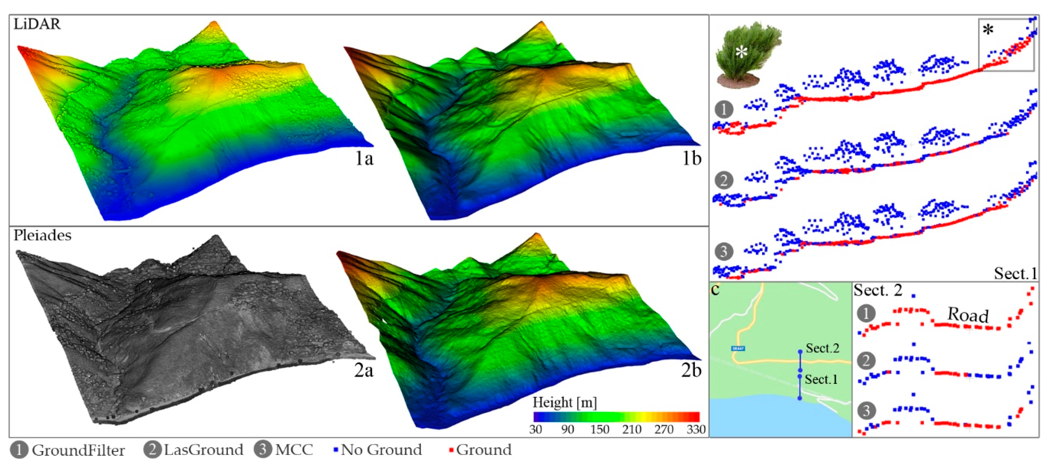
Figure 8 shows a comparison between the raw surfaces (panels 1a, 2a) and the filtered ones (panels 1b, 2b). In
Figure 8c, the planimetric position of two sections analysed in detail is reported, using the parameters considered best for each filter used. The red dots identify the profile of the filtered surface and the blue dots identify that of the original surface. As already pointed out, the algorithm that best interprets both the terrain and the anthropic areas (road) is the MCC (profile 3 of
Figure 8).
We have therefore decided to use the MCC algorithm to filter both data (lidar and HRSI) since it is the one that has brought the best results on both datasets.
5.2. Quality Assessment of the Grid Data, Outlier Identification and Detection
After filtering, the sample data was analyzed in order to detect any points that deviate significantly from the interpolated surface. The residuals have been computed as described in
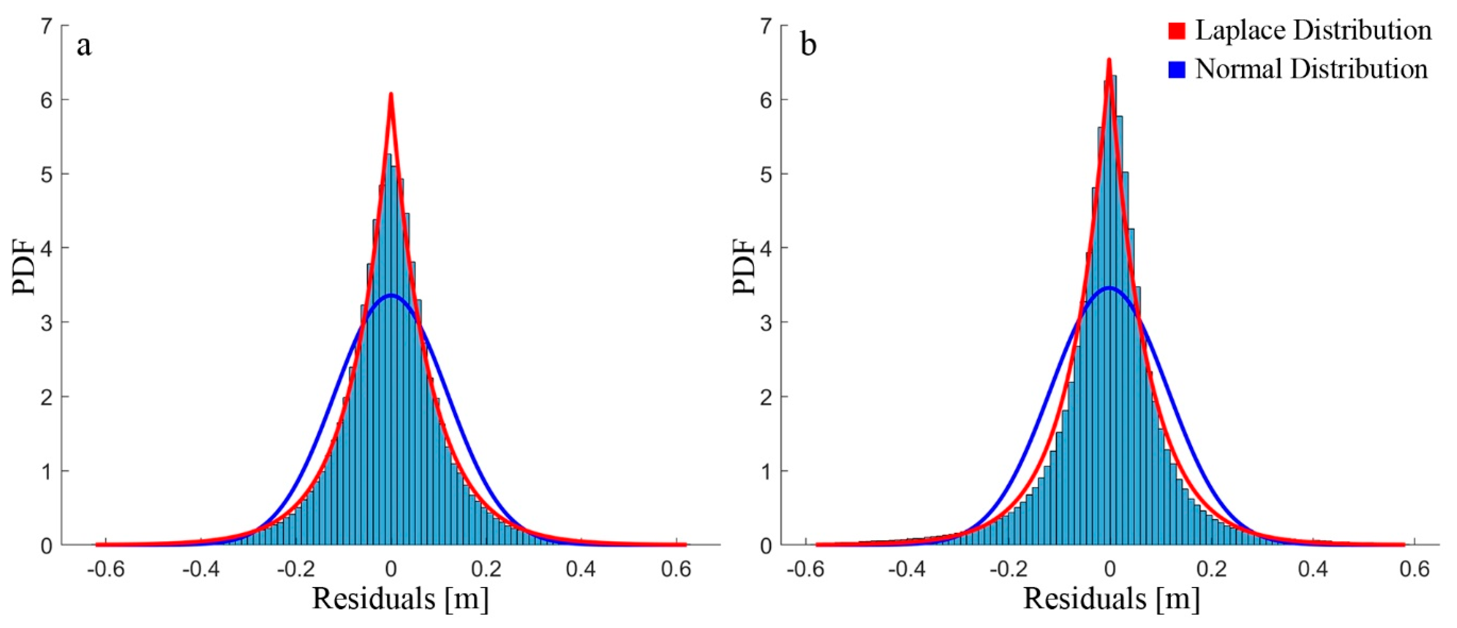
Section 4.2; the frequency histograms of the residuals are shown in
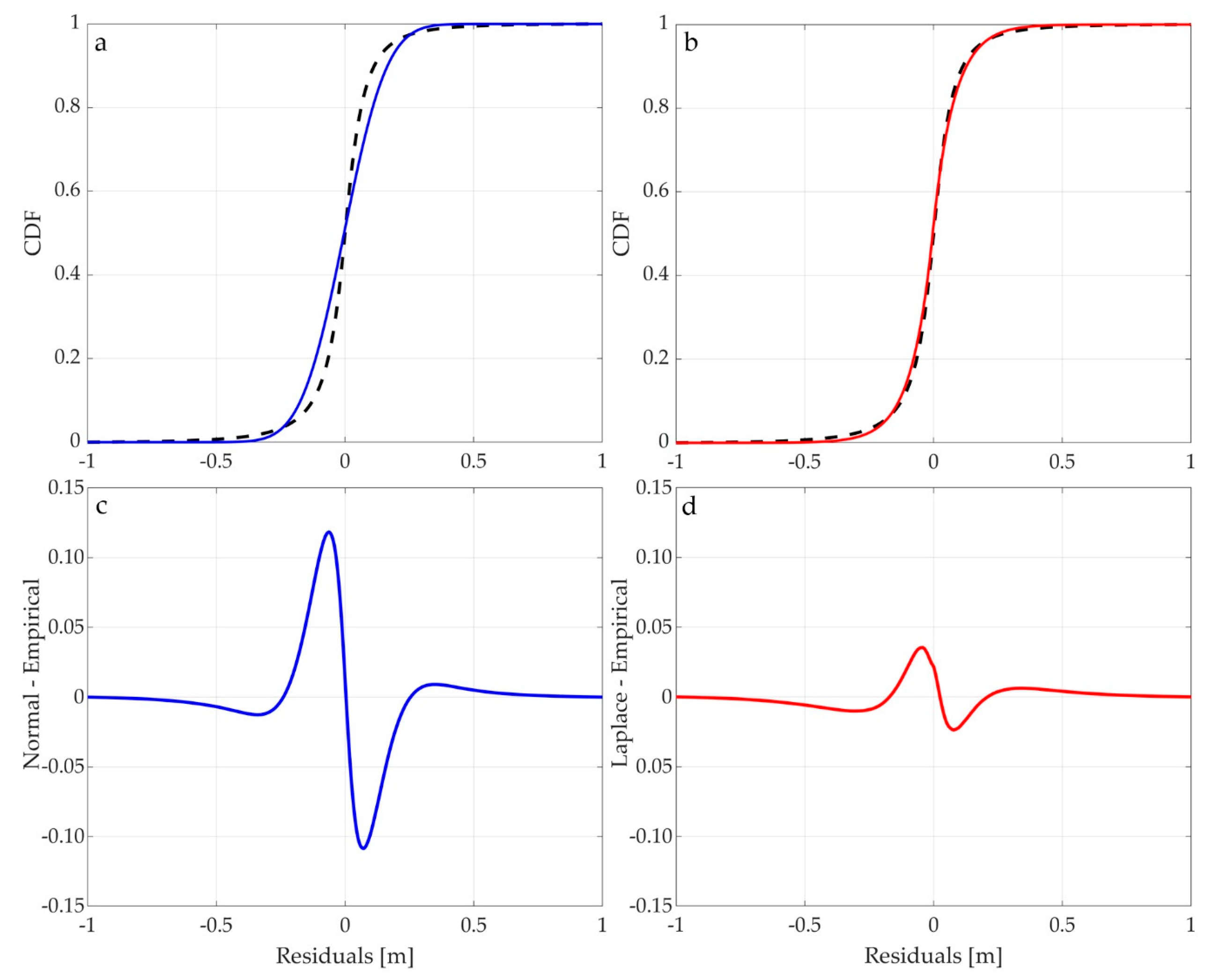
Figure 9. It should be noted that, for both lidar and Pleiades, they follow a trend that differs significantly from a normal frequency distribution. In the figure, the probability density function (PDF) curves of the normal (blue) and Laplace (red) distributions computed on the basis of the sample parameters are superimposed on the frequency histogram of the residuals.
Figure 10a,b respectively shows the cumulative distribution function (CDF) of the normal distribution and of the Laplace distribution superimposed to the empirical cumulative distribution. Since the empirical distribution and the Laplace are barely distinguishable, the differences between the distributions are reported in
Figure 10c,d (normal minus empirical and Laplace minus empirical, respectively).
In
Table 3 are given some statistical parameters for both the normal distribution and Laplace. Note that the kurtosis value of the samples is much higher (79 and 57, respectively) than expected for a normal distribution.
We ran a test of Kolmogorov Smirnov under the null hypothesis that the sample follows a certain distribution (once Normal and once Laplace). The null hypothesis Ho is rejected in both cases (the sample distribution is neither Normal nor Laplace). The parameters value of the statistics Kolmogorov–Smirnov (ksstat) and critical value, which are reported in
Table 4, are very different (ksstat is much higher for normal testing). We can therefore conclude that the trend of the samples (made up of 260,000 and 800,000 elements, respectively) is much closer to the distribution of Laplace than to a normal frequency distribution.
Once the distribution that best fit the trend of the residuals was estimated, it was possible to identify the confidence interval corresponding to a particular confidence level.
Table 5 shows the limits of the interval in relation to some confidence levels
p for the sample of lidar data; it should be noted that high values of
p (e.g., 99.5%) correspond to threshold values around 0.5 m. The identification of the confidence interval allows to remove from the sample some points resulting as outliers.
Table 6 shows, for a confidence interval of 99.9% and a cut value of 1 m, the limits, the number of outliers outside the limits (upper and lower), and the number of points within the interval.
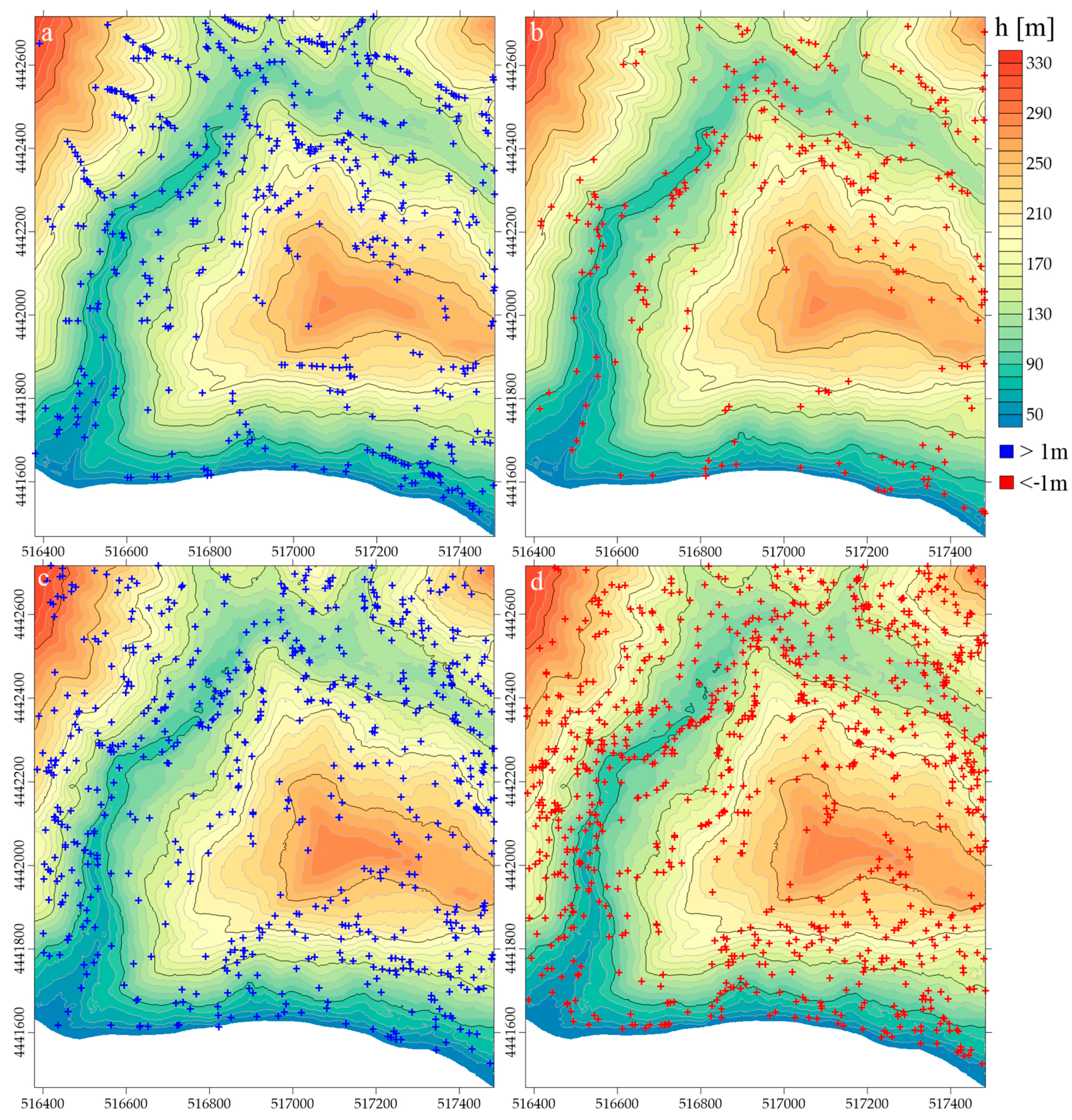
Statistical analysis has made it possible to identify outliers; this is important to understand their genesis. In order to facilitate the analysis of the data, wider limits have been considered to study only the highest deviations, greater in absolute value than 1 m; the positive deviations (
Figure 11a) and the negative ones (
Figure 11b) are reported in separate figures in relation to the lidar data only. In the case of Pleiades data, the filtered sample contains a greater number of points and even more outliers have been identified; those greater than 1 m in absolute value are shown in
Figure 8c,d.
5.3. Comparative Geomorphometric Analysis
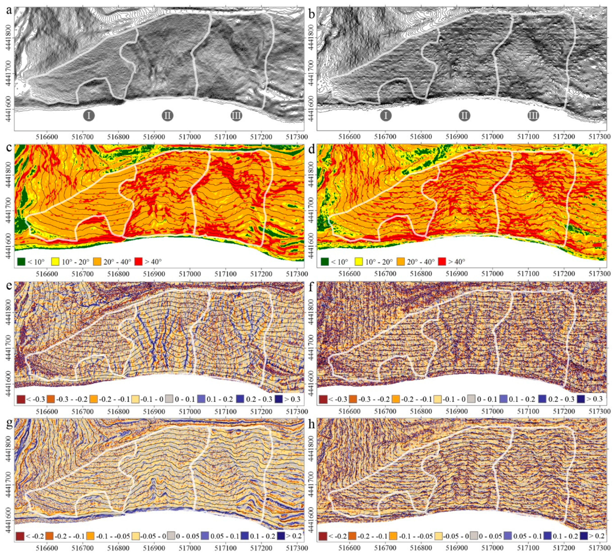
In order to analyze the surface of the terrain from a morphometric point of view, a series of feature maps derived from the DEMs can profitably complement the contour maps. Starting from the built grid DEM, we derived some feature maps: slope, plan, and profile curvature on the test area (
Figure 12). The slope maps have been reclassified into four classes: very gentle slopes for slope values <10°, gentle slopes for values between 10° and 20°, intermediate slopes for values between 20° and 40°, and steep slopes for values above 40°. The two types of curvature, plan and profile, were computed as the second derivative of the surface. The profile curvature is in the direction of the maximum slope, and the plan curvature is perpendicular to its direction.
Generally, values close to zero indicate a flat area; for this reason, the first class for plan curvature has been set between ±0.1 and 0 and, for profile curvature, between ±0.05 and 0. For both curves, positive values identify areas where concavity, in particular, planar curvature, which induces convergence of the surficial and sub-surficial flow, occurs for values equal to or greater than 0.3. Negative values, instead, identify convex areas, in particular, the planar curvature, which controls the divergence of the runoff and occurs for values equal to or less than −0.3.
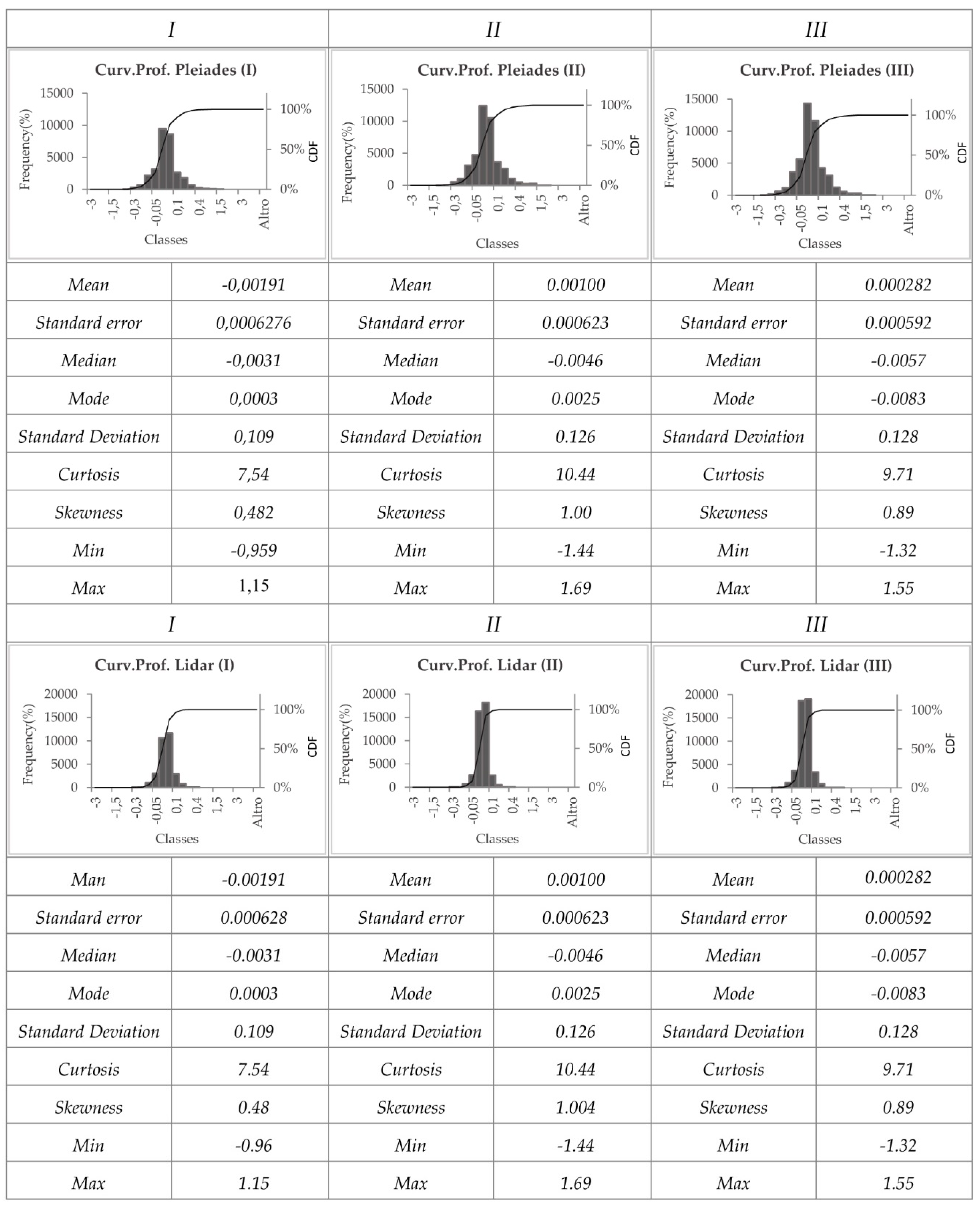
Afterwards, a geomorphometric analysis was carried out on the frequency distribution of the slope and curvature values (
Figure 13) separately for the three areas highlighted in
Figure 2, using comparatively the DEMs from lidar (2012) and Pleiades (2015). In the analysis of the three areas, the areas corresponding to the upper slope and the noses, considered not significant in the comparative analysis of the coastal slope, were excluded.
The angles of slope and the plan and profile curvatures are shown in the box plots of
Figure 13, where descriptive statistical parameters are summarized such as the upper, median, and lower quartile; mean; and maximum and minimum values. The values are categorized with respect to the three areas and for each DEM (green for lidar and blue for Pleiades).
The data set shows a wide range of variability. In particular, the slope derived from Pleiades has a standard deviation value that decreases from area I to area III, unlike the slope from lidar for which the standard deviation is comparable for the three areas. A considerable difference in the frequency distribution of the plan curvature values with regard to the lidar data is also evident; specifically, areas I and II have a smaller dispersion of values compared to area III. Instead, the range of variability of the plan curvature values relative to Pleiades is very wide but not too different for the three areas; the difference can only be seen in the extreme values of the three areas.
The profile curvature for lidar has very similar frequency distribution among the three areas, and this does not highlight the different geomorphological behaviors among them, unlike what happens to the plan curvature for Pleiades.
Figure 14,
Figure 15 and
Figure 16 show the slope, plan, and profile curvature distributions derived from the lidar and Pleiades base maps in order to evaluate how much each frequency distribution of data reflects the temporal variation of the morphologic processes that occurred in the three areas. For each map, the descriptive statistics parameters for the three areas are summarized. Moving from area I to area III, the topographic gradients show an increase in the amplitude of distributions that reflects the diversity of processes. In particular, a narrow distribution centered on a steep threshold slope, shown in Area I especially in slope values related to Pleiades data, indicates that only one or a few geomorphic processes occur (diffusion by soil creep modelling), as opposed to areas II and III which have a wider range of slopes than Area I, resulting from interactions between erosive processes and landslides, respectively. The distribution of the plan curvature of the maps from Pleiades for areas I and II shows a skewed distribution with respect to area III with a large distribution because the earthflow has shaped a large portion of the surrounding landscape. In fact, direct geomorphological surveys show that the landforms of area III are strongly influenced by gravity-driven processes. In most areas where several geomorphic processes overlap, the corresponding probability density distribution shows that the data are very dispersed around the mean value. For the distribution of data from lidar, in our case, the plan curvature values have a greater dispersion in area I (diffusion process) than in area III, where several overlapping geomorphic processes occur. For this reason, the authors believe that the distribution is not representative of the processes acting in the three areas.
The analysis of the profile curvature distribution, performed using the same classes, showed differences between the Pleiades and lidar data sources. The first shows an amplitude of distributions reflecting the increase in positive values (see continuous distribution function, CDF), while the second does not show an increase in amplitude of distribution. This condition may be due both to the excessive filtering of the lidar point cloud and to the different acquisition time of the remote sensed images (2012 and 2015) which reflect the evolution of geomorphic processes.
6. Discussion and Conclusions
The achievements of an appropriate level of accuracy in the processing of DEM from remotely sensed data is of certain interest for geodesy and topography [
48]. The analysis of the dynamics of geomorphic processes using the DEMs is one of the main interests of geomorphometry [
51,
52]. Finally, the use of both accurate DEM and quantitative geomorphometric results for geomorphological purposes enables the landform recognition and the development of landscape evolution models for research and engineering purposes [
32]. Often, the three disciplines operate separately and sometimes are in contrast, as discussed in Reference [
48]. As effectively pointed out by Sofia et al. [
53], geomorphometry analysis is a twofold process of knowledge: i) data extraction and accuracy assessment consider that error propagation in derived maps must be minimized as the usefulness and validity of geomorphometric applications are strongly related to the quality of the original data used; ii) these optimized data are used to derive basic and compound indices for mapping and modelling specific processes of interest. They also outline the advantages and disadvantages of each disciplinary approach as well as the existence of significant weaknesses and limitations due to cascade-like cognitive processes (multidisciplinarity).
In our opinion, a true interdisciplinarity could instead guarantee more robust methods and better results, overcoming the separation between field-based, grid-based, and object-based methodologies. Consistent with this premise, a fairly relevant result of our research and its application on a test case, which we would like to discuss in this section, concerns an indirect result of the interdisciplinary research (geomatics, geomorphometry, and geomorphology) that we have performed. According to Guida et al. [
54], the results of this interdisciplinary research based on the so-called GmIS_UNISA method combined with the accuracy analysis of the maps [
48] show that the peer-to-peer approach between the judgement based on geomorphological experience and the analysis of geomatics greatly improves the subsequent geomorphometric computations and the final morphogenetic, morpho-dynamic, and morpho-chronological interpretations. This confirms the call launched by Sofia et al. [
53] for best practices in all disciplines, highlighting new technical developments and showing innovative applications of geomorphometry to multiple applications and practices of engineering geomorphology.
The results of our analyses, already discussed in the previous section, show how an overall difference between areas with different rates of geomorphic evolution and current processes correspond to different geomorphic signals and geomorphological space–time signatures.
Figure 17 shows the contour line maps plus the positions of the points characterized by residual values greater than 1 m (both in positive, blue crosses and in negative, red crosses), considered outliers. Analyzing the residuals, it is possible to notice how specific combinations of the same represent specific configurations of ongoing erosive processes. The combined erosive action of runoff and sub-surficial flows is most concentrated in the areas of greatest erodibility and incohesiveness, corresponding to bedrock beds and joints and/or loose debris horizons, where the processes of subsurface erosion such as sapping are accelerated. The analysis of the maps allowed the expert judgement to identify specific natural and anthropic geomorphic features recognizable through outlier configurations, also known for the direct surveys that were carried out in situ. For both datasets (lidar and Pleiades), the areas with the highest percentage of negative values are the most anthropized. For example, such negative values are often found in areas where road cuts and fills have been made. It should be noted that the map of the left panel of the figure is related to the analysis of outliers on the 2012 lidar data, apparently characterized by greater accuracy, while the map of the right panel is related to the 2015 Pleiades data.
A comparative analysis can be useful to discriminate possible errors in the building of DEMs from real geomatic signals caused by changes in the topography of the land that occurred from 2011 to 2015. In order to better explain the above concept, two areas related to maps derived from lidar, (boxes 1 and 2 on the map) have been analyzed in more detail. Also, in
Figure 17, for area 1, we show the location of a particular cluster of outliers, upstream from the coastal cliff (panel 1a). In correspondence with the section drawn on the map excerpt (panel 1a), panel 1b shows the point cloud in longitudinal profile. Note the overlapping and/or adjacency of positive (below DEM) and negative (above DEM) residuals. It is clear that there are two overhanging topography, one upstream attributable to erosive processes such as sapping and the other downstream to the undermining of the coastal cliff due to the action of sea waves. The simplified scheme of the sapping erosive mechanism is shown in panel 1c. The overhanging at the most erodible horizons is evident in the photograph shown, of which the camera position is shown in the figure. Moreover, areas with only positive residual values identify particular configurations that can be interpreted as tension crack systems or small trenches. Panel 2b shows the longitudinal profile of the point cloud at the section line drawn on the excerpt of the map in panel 2a, orthogonal to a series of aligned positive outliers. Note that the outlier (blue point) is located at the base of the fracture. The practical feedback attributes to this configuration tension cracks formed as a result of the landslide movements in evolution downstream (see scheme in panel 2c).
We have noted that the geomorphometric analysis of outliers, identified by statistical criteria, allows to identify and characterize the existence of a correlation between a number of alignments and clusters of outliers and some main geomorphological characteristics (or groups of main characteristics), which are significant for the recognition of the landform elements and the definition of specific processes. In other words, the outliers identified very often seem to correspond to morphological characteristics, which suggests that they may not be filtering errors or other gross errors.
The study on geomorphometric analysis is consistent with the expert geomorphological interpretation of the evolution processes that act on the three areas under study and confirms what has already been highlighted by other authors such as Iwahashia et al. [
28] and Booth et al. [
26]. The use of derived maps, slope and the plan and profile curvatures, represent the geomorphological expression of the evolution in progress according to the laws of diffusion and advection that depend respectively on the curvature and slope. The frequency distribution of the values of these maps shows, especially for the slope, a platykurtic form in passing from an area with lesser processes of alteration and erosion to an area completely modified by landslide processes; at the same time, even the standard deviation is greater given the overlap of the different erosive and geomorphic processes that coexist on the same area [
26].
Another aspect that we would like to highlight and discuss concerns the filtering of point clouds in order to build a DEM corresponding to the bare ground (therefore, a DTM) as a result of interpolation processes. All three filter methods tested have been developed for lidar data. The points of the cloud that go beyond the vegetation and correspond to the bare ground are, in this case, more numerous than for the photogrammetric data, where the point cloud comes from a processing of images acquired from passive sensors. For this reason, the filtering of lidar data was more effective and the DEMs and maps derived from them were better, although the data was less resolute than the photogrammetric one.
The filtering method that gave the best results, for both data sets, is the MCC. The two main parameters to set are the scale parameter λ and the curvature threshold
t. The results depend strongly on their correct balance. However, since the scale parameter is to be set to a value having the order of magnitude of the resolution of the input data and the resolution of the lidar data is not homogeneous, its choice in this case is not trivial. Once a certain scale parameter has been set, the process is run iteratively in a range of values between 0.5λ and 1.5λ until convergence is reached. Our tests show how effectively the optimal scale parameter is a function of the resolution of the input data, in our case, equal to the value suggested in the guidelines (0.55 m). As far as the tolerance value chosen following the results obtained is concerned, it is much higher than the default value (0.095 instead of 0.05) and is due to the uneven morphology of our area and to the presence of the Mediterranean scrub on steeply sloping areas. To use the same algorithm on the photogrammetric data, it was necessary to set a scale parameter much higher than the average resolution of the data; this involved the removal of large areas in areas with high vegetation density. It has also been shown that, even in the areas of bare ground adjacent to the high-stemmed vegetation, the reliability of the points of the photogrammetric cloud is still lower than that of the points of the lidar cloud in the same area. This is evident by observing the maps of the FOM (correlation index of the images) shown in
Figure 5; in proximity of the wooded areas or with medium/high vegetation, the values of FOM are around 40% while lower values (around 20%) are in the areas near the vegetation due in particular to the effect of the shadows produced by the same. The most reliable areas, in line with the results from lidar, are the stable ones, in correspondence with those that have not in ancient times undergone major displacements.
Figure 18 shows the classified map of the differences in absolute value of elevation of the filtered point clouds, in correspondence to zone I of
Figure 12. The uncertainty of the differences in elevation can be estimated to be about 0.97 m, taking into account those associated with the two data sets (15 cm for ALS, 47 cm for HRSI). Differences of less than 1 m were therefore not considered significant while greater differences can be attributed to erosive processes. From these considerations, it results that the data coming from photogrammetric point clouds in areas where vegetation is not present allow a more effective identification of some of the main features, as shown in
Figure 17, especially because of the higher resolution of the point cloud.
The presence of a higher percentage of outliers (
Figure 11 and
Figure 17) in the photogrammetric data is also due to the higher resolution of the data in non-wooded areas while, in wooded areas, the presence of outliers is due to the excessive “smoothing” of the point cloud as a result of a failed filtering. For these reasons, the expert judgement focused on tracing the features in correspondence with the only reliable zones. Based on what we have been discussing, a hypothesis of research line for future activities in the geomorphological field arises. Starting from the results of morphometric analysis, these activities aim at the objective multi-temporal identification of landforms (object-based landforms recognition) according to a hierarchical and multiscale approach in line with the geomorphic phenomena identified in the study areas. The reinterpretation of outliers in geomorphic terms is an interesting field to be explored in order to optimize and automate the recognition of certain landforms, which are currently difficult to recognize on an objective basis. It is therefore planned to continue the geomorphological interpretation of outliers and the identification and delimitation of geomorphic elements such as sapping or cracks, which is difficult to achieve on excessively filtered cartographic bases that, at the same time, eliminate values that would seem anomalous on statistical and topographical bases but which have a real match with the field surveys.

 ,
, 


