Capital Preservation and Current Spending with Sovereign Wealth Funds and Endowment Funds: A simulation Study

Abstract

We simulate the future performance of the Norwegian Government Pension Fund Global as a leading example of sovereign wealth funds intended both to preserve wealth and provide regular budget contributions. Withdrawals are limited to the fund’s expected real returns; however, deviations are allowed to fund automatic stabilizers as well as discretionary fiscal policy. It also allows smoothing to avoid abrupt changes. Except for the fiscal policy part, many endowment funds are subject to similar rules. The main findings are: (i) Even if withdrawals matching expected returns maintain the fund’s value in expectation, the fund will be depleted eventually. (ii) Because the fund is invested in foreign currency, long-run purchasing power parity introduces an element of mean reversion and hence a negative serial correlation in the rates of return, so that the fund’s value is not even preserved in expectation. (iii) The use of the fund for fiscal policy introduces a substantial risk of depletion in finite time. (iv) Smoothing raises the risk of depletion after large negative financial returns, though only modestly so. Risk reduction and withdrawal rates below expected returns are explored as remedies. Risk reduction postpones the eventual depletion but does not eliminate it. Lower withdrawal rates help sustainability more fundamentally, but bounds on fiscal policy are needed for depletion risk to be eliminated.

1. Introduction

Recent decades have seen a wide buildup of government-owned investment funds, commonly called sovereign wealth funds (SWF). As discussed by Braunstein (2022), the context of their origins varies. In some cases, such as a number of Asian countries, they have emerged from large export surpluses, especially after the Asian financial crisis in 1997–1998. In another important set of cases, they serve as deposits of temporary government revenues from the harvesting of non-renewable natural resources, such as oil and gas in Norway, Australia, and the Middle East, or copper in the case of Chile. In a third set of cases, such as Singapore, Hong Kong, and some Persian Gulf countries, they have resulted from domestic debates and power struggles on how to organize domestic finances after independence from former colonial powers.

The purposes of establishing SWFs vary as well. For natural-resource states, the saving objective typically dominates, i.e., preservation of wealth for future resources. Stabilization in response to natural-resource price fluctuations and other macroeconomic disturbances frequently is added to the saving objective. In many cases, especially in emerging economies, domestic development, such as investment in infrastructure, may be more important than financial saving. Finally, a number of developed economies, such as France and Italy, have established SWFs as instruments of industrial policy, including ensuring national ownership of key companies.

Investment strategies naturally vary as well. Some funds, such as Singapore’s Temasek, focuses on direct ownership in global companies. Others, such as many Arab SWFs, concentrate their ownership in domestic strategic industries, as studied by Arouri et al. (2018). A third group, including Singapore’s GIC and Norway’s Government Pension Fund Global, do not own their assets, but manage global financial portfolios on behalf of their respective governments.

As a group, and in some cases individually, SWFs are large enough to affect the functioning of global financial markets. Boubaker et al. (2018) investigated their effects on equity prices. Baldwin (2012) discussed their political as well as financial impact in a historical context. Other important contributions include Alhashel (2015); Bernstein et al. (2013); Paltrinieri and Pichler (2013); Dreassi et al. (2017); and Johan et al. (2013).

This paper focuses on the issues and tradeoffs facing a SWF with a dual objective of saving for future generations and the stabilization of government finances. The case we study is the Norwegian Government Pension Fund Global (GPFG), currently the world’s largest SWF with assets under management of about USD 1.3 trillion. The tradeoffs result because, on the one hand, this fund is to be managed so as to preserve the wealth for future generations while, on the other hand, its financial returns are supposed to provide partial funding of government budgets on a regular basis. This raises not only the question of how large these contributions can be, but also about how they may or may not vary over time because, as argued by Barro (1979) and others, tax rates and public services ought to move smoothly.

With a complete representation of fund-owner preferences regarding these and other tradeoffs, we should be able to derive the optimal strategy for investing the fund and spending of the proceeds. Any such presentation would necessarily be complex and might not even be well defined considering that the relevant decisions are made by groups whose members might have conflicting interests. Furthermore, rational decision making is made difficult by the complexities of the consequences of many owner actions. We believe this makes a case for studying the implications of observed fund-owner behavior. In this paper, we do this by simulating the likely consequences of the rules and practices that have been implemented for the GPFG.

The relevance of these kind of tradeoffs is not limited to this kind of SWFs but is shared by a large number of private funds, especially endowment funds of private universities, museums, and the like, and to some extent also pension funds although they have less flexibility regarding payment obligations. We thus believe our results should be relevant for the management of such funds as well. University endowment funds have been studied, for example, by Barber and Wang (2013); Brown et al. (2014); and Dahiya and Yermack (2018).

The GPFG Act of 1990 (with subsequent amendments) stipulates its purpose as preserving the government’s temporary revenue from oil and gas extraction for future generations. A regulation passed by the Storting (Parliament) in 2001 furthermore stipulates the rules for spending of the fund’s proceeds. They can be summarized as follows:

• As a main rule, an amount corresponding to the fund’s expected financial return can be added to each annual budget. The expected rate of return was stipulated as 4 percent in 2001 and lowered to 3 percent in 2017.
• The rule applies to the structural budget balance, meaning that the rule does not restrict the funding of automatic fiscal stabilizers, whether positive or negative.
• Additional fiscal spending can be financed by the fund if desirable for stabilization of domestic business cycles, provided similar tightening is undertaken in good times.
• Smoothing can be applied to avoid sharp changes in annual withdrawals.

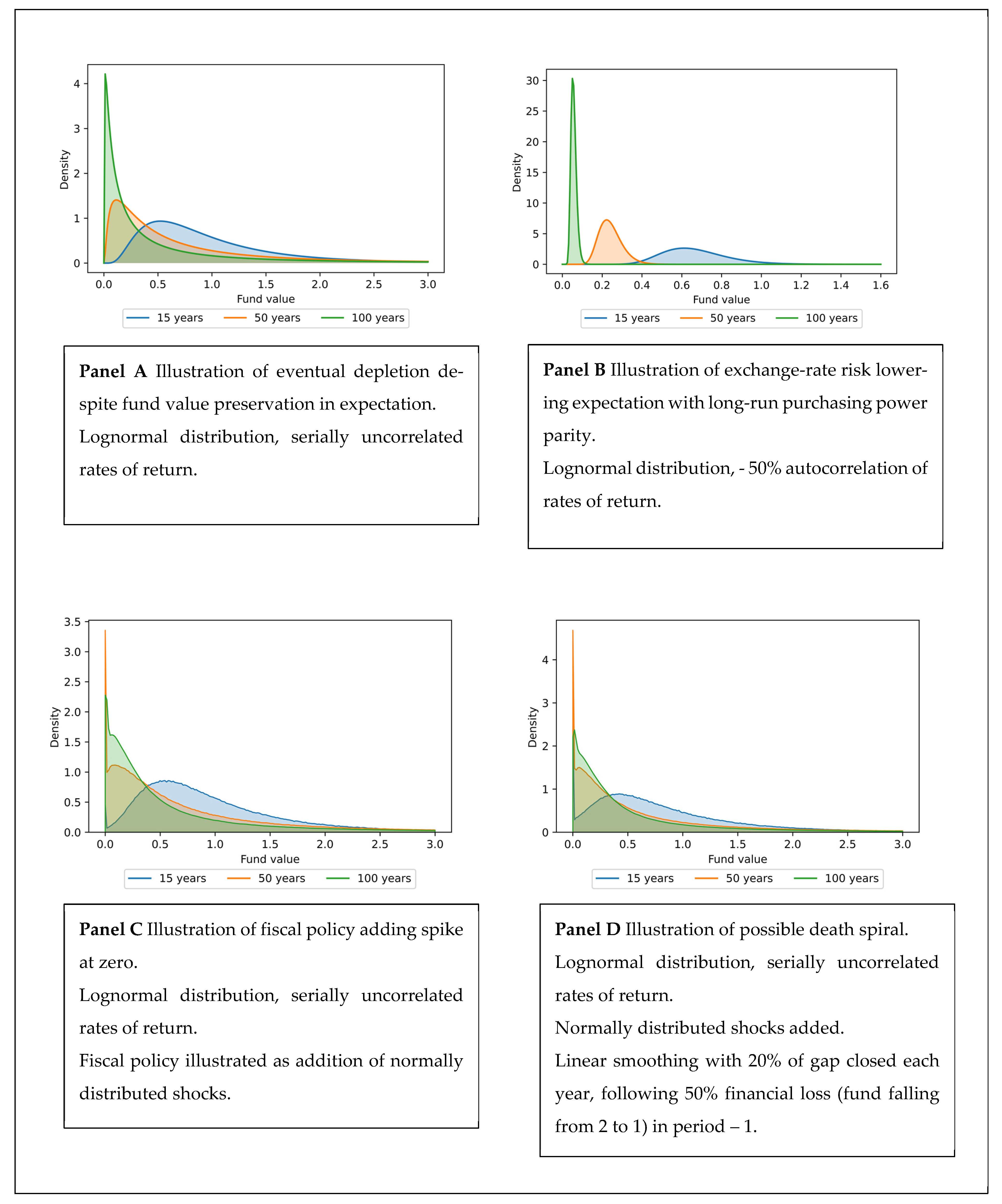
This paper simulates the likely implications of the practices based on this set of rules over time. We base the simulations on an econometric model of fiscal behavior and the relevant financial variables, estimated on data for 1991–2020. Our simulations reveal a number of challenges, illustrated in Figure 1, that arise from the observed behavior.

First, although the main rule of spending only the expected return is intended to maintain the fund’s value for future generations, it does not meet that intention. At best, it preserves the expected value, but with a variance that rises with the time horizon. However, preservation of the expectation does not make preservation of the current value likely. To the contrary, by concentrating more and more of the probability distribution next to its zero lower limit, it eventually depletes the fund with a probability approaching unity.

Second, because the fund is invested globally, but the proceeds spent locally in the national currency, exchange-rate risk with long-term purchasing power parity introduces an element of mean reversion and hence a negative serial correlation in the rates of return in the national currency. Then, the fund’s future value is not even preserved in expectation.

Third, the use of the fund for fiscal policy adds an additional risk factor, which may be positively correlated with financial market movements. Moreover, because fiscal actions tend to be normally rather than lognormally distributed, they are likely to widen the fund value probability distribution symmetrically except for a spike at zero, thus raising the risk of future depletion.

Fourth, smoothing after a major loss means that withdrawals as a percent of fund value will increase at the same time as fund value falls. That raises the question of whether the fund can be caught in a “death spiral” that make depletion unavoidable.

Although the fourth point does not seem a major threat, our results indicate that the first three of these challenges are quantitatively important for the Norwegian GPFG. However, we also propose remedies. Reducing financial risk taking by lowering the equity share to 50 percent from the current 70 reduces the need for smoothing of the withdrawals by smoothing the development of the fund itself. It also delays the tendency for the probability mass to be concentrated near zero but does not eliminate it. A better remedy for that problem would be to reduce the withdrawal rate to 1.5 to 2 percentage points below the expected return. Both remedies would result in lower withdrawals in early years, but this effect may be reversed over time, especially with a lower withdrawal rate, because the fund then is allowed to grow faster.

Reducing or eliminating the depletion risk associated with fiscal policy would require stricter limitation of the scope for fiscal stimulation during the recessions. Whether or not such limitations would be worth the cost of sharper recessions depends on policy makers’ preferences.

Fiscal sustainability is naturally at least as important for governments whose financial operations are mainly on the liability side of the balance sheet. Our paper is thus related to the vast literature on public debt, with Blanchard’s (2019) Presidential Lecture as a recent example. However, the issues faced by governments with negative financial wealth lie beyond the scope of this paper. We also do not go into the issues that arise for a government that draws down its financial wealth and starts borrowing.

Our paper adds to the literature on the tradeoffs involved in the management of persistent, yet temporary revenues from non-renewable natural resources, such as the studies by van der Ploeg and Venables (2011); van den Bremer et al. (2016); and Irarrazabal et al. (2020). However, unlike the former, we do not focus on developing economies. Unlike the latter two, we ignore the prospect of future fund deposits and focus instead on the management of and spending of revenues from the fund proper. Our approach is similar to the one taken by Lindset and Matsen (2018) but goes deeper into the consequences of the strategy set up by a government such as Norway’s. Unlike Aase and Bjerksund (2021) and Lindset and Mork (2019), we do not seek to derive optimal results, but seek instead to uncover the implications, perhaps unintended, of decisions actually made.

The rest of the paper is organized as follows. Section 2 gives a conceptual introduction to the challenges of long-term investing. Section 3 presents the relevant data and our time-series model of fiscal behavior and financial returns. Section 4 presents the simulation model, including our specification of the Norwegian fiscal rule. Section 5 presents the main simulation results, and Section 6 presents the implications of smoothing. Section 7 presents and discusses the possible remedies for the challenges that our analysis uncovers and Section 8 concludes the analysis.

2. Some Inconvenient Truths

The Norwegian fiscal rule allows annual withdrawals corresponding to the expected real return on the fund. Similar rules are practiced by a number of endowment funds. Such rules are intended to guarantee preservation of the fund for future users and generations. The intuition is as simple as it is appealing: By spending only the return, the principal is preserved.

In the absence of risk, this intuition is correct. With risk, returns will fluctuate around its expected value, but the fluctuations should average to zero over time, as suggested by the law of large numbers. It would then seem to follow that the value of the fund should be preserved over time as well. That turns out to be true only in a very limited sense. That is, provided the rate of return is serially uncorrelated, the fund value will be preserved in expectation; however, the preponderance of probability is for the fund to gradually lose value over time. Furthermore, this preponderance rises with the time horizon. Eventually, the fund will be depleted with a probability approaching unity.

The main explanation for this result, which was proved by Dybvig and Qin (2021) and presented in the context of the Norwegian GPFG by Aase and Bjerksund (2021), is that the law of large numbers applies to sums, not products, and the dynamic development of an investment fund depends on products of the type:

$$A_{t+1}=\left(1+r_t\right)\left(A_t-D_t\right),$$

(1)

where $A_t$ denotes the fund value, $D_t$ withdrawals, and $r_t$ the rate of return. Simply put, a 50 percent loss is not canceled out by a subsequent 50 percent gain. Although the effects of gains and losses will outweigh each other in expectation, the probability distribution of future fund values become increasingly skewed to the left the further one looks into the future. The increasing uncertainty is a case of a mean-preserving spread. Whereas spreads to the right (toward higher values) are unlimited, spreads to the left (towards lower values) are limited by the lower bound of zero, an absorbing barrier1. So, as the time horizon increases, more and more of the probability mass will agglomerate at values very close to zero. The expectation will be preserved by the possibility of extremely high values, but with low probabilities. In the limit, the entire probability mass collapses into a spike next to zero.

Formally, assume normally distributed and serially uncorrelated returns with constant means and variances in continuous time, so that $r\left(t\right)~\mathcal{N}\left(\mu ,{\sigma }^2\right)$. Withdrawals from the fund are made at the constant rate of $\delta$. Then, as proved by Dybvig and Qin (op. cit.), the expectation at time zero of the fund size $A\left(t\right)$ at a future time $t$, relative to the original fund size $A_0$ is:

$${\mathbb{E}}_0\left(\frac{A\left(t\right)}{A_0}\right)=e^{\left(\mu -\delta \right)t},$$

(2)

which is unity provided $\delta =\mu$.

Thus, withdrawing an amount corresponding to the expected return does indeed preserve the fund in expectation. However, with $\delta =\mu$, the probability of the future fund value falling short of an arbitrary positive number $a$ is:

$$P\left(A\left(t\right)<a\right)=\frac{1}{2}\left[1+\mathrm{erf}\left(\frac{\ln a+\frac{1}{2}{\sigma }^{2}t}{\sigma \sqrt{2t}}\right)\right],$$

(3)

where $\mathrm{erf}$ denotes the Gauss error function. Clearly, for $t\to \infty ,$ $P\left(A\left(t\right)<a\right)\to 1$. Thus, as the time horizon grows, the distribution will become increasingly more skewed to the right until all of its mass is concentrated near zero.

The increasing uncertainty as the time horizon grows takes the form of a mean-preserving spread. However, whereas this spread faces no upside limits, the downside is limited by the lower barrier of zero. So, although the mean remains preserved, an increasing accumulation of probability mass just above zero is balanced by some very high outcomes. However, the probability of the very high outcomes becomes increasingly small and eventually vanishes, so that the fund eventually is depleted almost surely. The only way to maintain sustainability is to withdraw a fraction that is lower than the expected return2, i.e., $\delta \le \mu -\frac{1}{2}{\sigma }^2$.

If the rates of return are negatively serially correlated, withdrawals equaling the expected return will not even preserve the fund’s value in expectation. Negative serial correlation arises if the fund is invested in securities denominated in a foreign currency (e.g., U.S. dollars), withdrawals are made as a fixed fraction of the fund’s value in the domestic currency (in our case, Norwegian kroner), and the exchange rate obeys purchasing power parity for the long term. Then, the real exchange rate can be modelled in continuous time as an Ornstein–Uhlenbeck process in logs, i.e.,

$$dv=\alpha \left(\kappa -v\right)+{\sigma }_{v}d{B}_v,$$

(4)

where $v$ is the log value of the foreign currency. As shown in a companion note (Mork and Trønnes 2022), the expectation at time zero of the relative fund size $A\left(t\right)/A_0$ then becomes:

$${\mathbb{E}}_0\left(\frac{A\left(t\right)}{A_0}\right)=e^{-\frac{1}{2}{\sigma }_v^2\left[t-\frac{1}{2\alpha }\left(1-e^{-2\alpha t}\right)\right]}<1.$$

(5)

The intuition behind this result starts by noting that the change of currency introduces a second risk factor for the fund in addition to the return risk in the global asset markets. Furthermore, unlike the risk from the global financial markets, the upside part of that risk is limited by the mean reversion implicit in the purchasing-power parity condition. As a result, not even the mean is preserved over time.

Purchasing power parity means that the real exchange rate is stationary in the statistical sense. The question of stationarity versus a unit root has not been settled in the literature. The well-known difficulty of reliably forecasting future exchange rates, as noted by Meese and Rogoff (1983) and further analyzed by many others3, supports a unit root. In our data, a unit root can be rejected with borderline significance, as explained in the next section. On an extended sample, going back to the end of the Bretton Woods system in 1971, the rejection becomes barely significant at the 10 percent level. In our simulation exercises, we find that a unit-root assumption results in projections of future real exchange rates that in some cases are too high and in other cases too low to be credible. When added to the long-sample econometric data and the theoretical purchasing-power argument, this convinces us to specify the real exchange rate as stationary.

Further complications arise if the fund owners allow occasional deviations from the fixed withdrawal rate. Endowment fund owners may, for example, permit larger draws at times where other sources of revenues, such as tuition or ticket sales, are lower than normal. Extraordinary SWF withdrawals may be used to maintain public services whenever tax revenues fall because of recessions, as codified in the Norwegian fiscal rule. Discretionary fiscal action to stabilize the economy may be added. A minimum requirement for such extraordinary draws to be sustainable would be that they are reversed in good times, statistically speaking that they are distributed symmetrically around zero. We consider it reasonable to view such withdrawal variations to be normally distributed rather than the typically lognormal distribution for the regular gross withdrawals. The support of the normal distribution is not limited by zero on the downside. However, we do not allow the fund value to fall below zero4. As a result, the distribution for the future fund value becomes a hybrid of a lognormal and a truncated normal with a spike at zero. Thus, the fund may be depleted in finite time and not just eventually.

3. Data and Time-Series Model

Simulation of fund behavior over time requires model specification of the time series behavior of financial returns as well as the fiscal variables that determine withdrawals. We estimate this behavior from historical data. Because the fiscal data are available on the annual frequency only, we use annual data for all our series.

For the financial data, we start by noting that the fund’s equity and fixed-income decisions are required to closely follow the FTSE Global equity index and the Bloomberg bond index, respectively, data for which our colleague Espen Henriksen graciously shared with us. Unfortunately, these index series are only available from 1991 on, which limits our sample to the 1991–2020 period. We thus base our moment estimates for the fund distribution on data for the total-return development of these indices. For each series, we compute annual nominal returns in U.S. Dollars (USD) as the log difference between the end-of-year values for the respective index values. We then deflate them by the December-to-December log changes in U.S. CPI (downloaded from the FRED database) to obtain real USD returns. For the exchange rate, we use the year-end daily bilateral USD/NOK nominal exchange rates, obtained from the Norges Bank, and deflate them by the December values of the relative U.S.-Norwegian CPI, the latter downloaded from Statistics Norway.

Data for the relevant fiscal data were available in the Norwegian government accounts (Statsrekneskapen). Because all non-oil deficits5 on the government budget are required by law to be covered by fund withdrawals for as long as there is money in the fund, the time series behavior of the withdrawals is identical to that of the non-oil deficit.

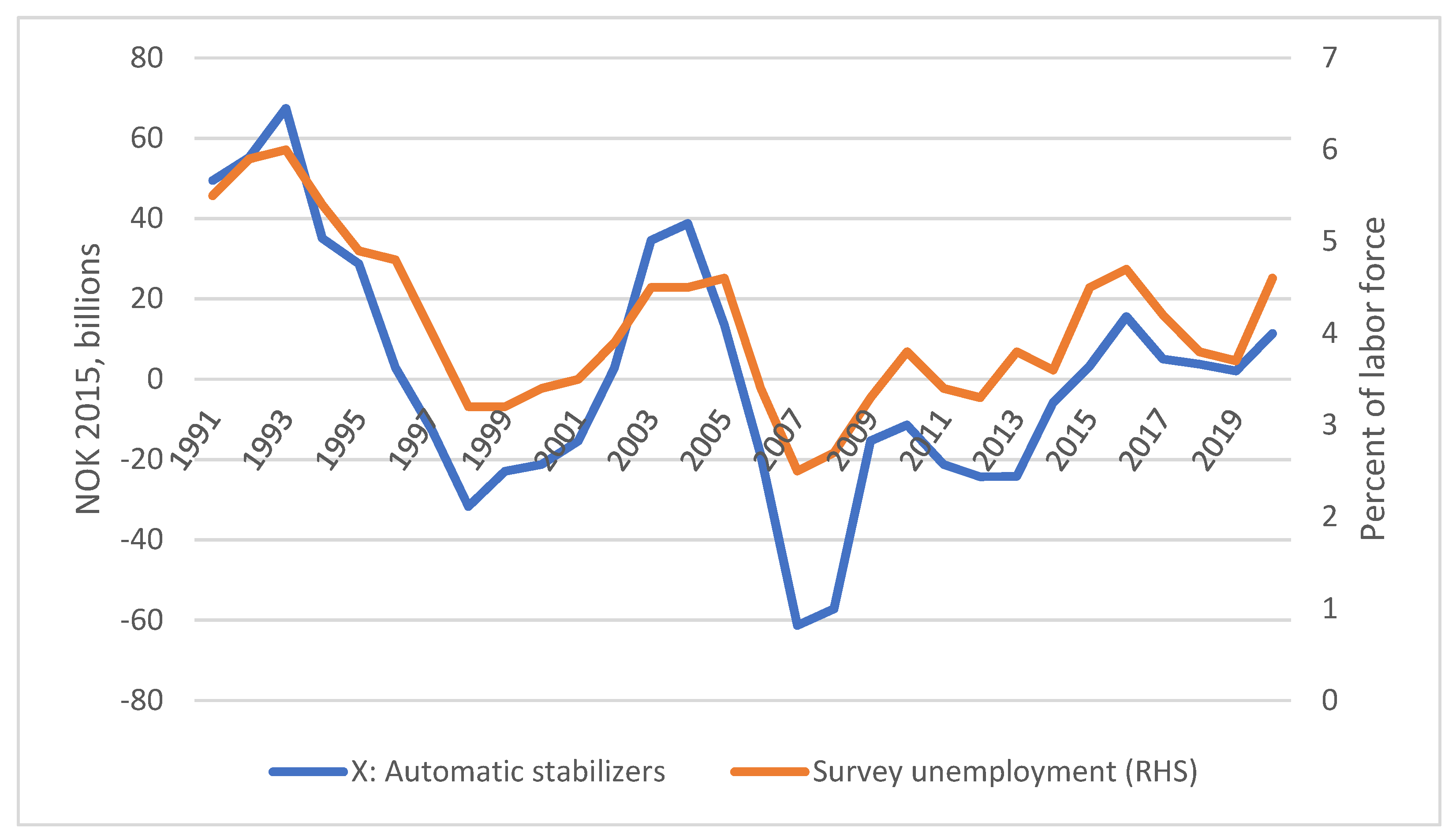
This deficit is furthermore decomposed into a structural and a cyclical component according to a set of algorithms developed by the Ministry of Finance. The cyclical component is supposed to represent the contribution—positive or negative—that is purely due to the cyclical movements in the overall economy and thus not caused by changes in tax rates or entitlement rules. Typically, recessions reduce revenues because incomes fall and increase expenditures on unemployment benefits, and vice versa. These movements are also referred to as automatic stabilizers. We denote this magnitude as $X_t$. Data for this variable, which may take on negative as well as positive values, can thus be taken directly from the government accounts6. As shown in Figure 2, the movements of this variable closely parallel those of the ILO-compatible survey unemployment. It can thus be interpreted as a fair (though inverse) representation of the Norwegian business cycle.

The automatic stabilizers can be interpreted as the cost of maintaining a smooth flow of government services in the face of cyclical variations in tax revenues and expenditures such as unemployment compensation. Foundations face similar challenges, wanting to maintain services and other activities, such as museum exhibitions or university teaching and research, at times when revenues from sources other than the endowment fund temporarily fail to arrive in their usual amounts. Recessions may, for example, hurt ticket revenues, charitable giving, student enrollment, or government funding. Thus, the presence of our variable $X$ does not limit the validity of our analysis to governments.

Fiscal spending or tax cuts, aimed at stabilizing the overall economy, is specific to governments, however. The specification of the rules governing Norwegian fiscal policy requires some care. The fiscal rule, introduced in 2001, allows the government to normally run a structural, non-oil deficit corresponding to the expected return on the fund, defined as the fund’s value at the beginning of the year multiplied by the expected rate of return. Letting $\overline{r}$ denote this rate and $A_t$ the beginning-of-year value of the fund, this normal, structural, non-oil deficit is defined as:

$${\overline{S}}_t=\overline{r}{A}_t.$$

(6)

However, the Storting (Parliament) may exceed this limit if the cyclical situation calls for discretionary fiscal stimulus, provided this excess is compensated by subsequent tightening as the economy normalizes. Letting $F_t$ denote the discretionary spending (or tax cut), the realized structural, non-oil deficit can then be written as the sum:

$$S_t={\overline{S}}_t+F_t,$$

(7)

where $F_t$ can have either sign.

The government accounts contain data for $S_t$ but not $F_t$. We construct them by using the formula in Equation (6) for ${\overline{S}}_t$ and subtract the resulting series from $S_t$. For 1991–2001, before the fiscal rule went into effect, we stipulate ${\overline{S}}_t=0$, so that $F_t=S_t$. For the subsequent years, we use ${\overline{S}}_t=\overline{r}{A}_t$. However, the official estimate for $\overline{r}$, which was stipulated at 4 percent for the 2001 decision, was cut discretely to 3 percent in 2017 for budgets from 2018 on. This cut came after a lengthy public debate starting with a speech7 by the Central Bank Governor in 2012, where he argued that the persistent decline in global interest rates called for a lower estimate. Although the Governor’s proposal at first was rejected by elected officials, the debate continued. During this debate, structural, non-oil deficits were persistently kept well below the bar set by the 4 percent criterion, by increasing margins. We interpret this trend as a growing realization that the 4 percent estimate had become excessive. For example, in its budget proposal for 2017, the Government warned8 that the real return likely would be lower in subsequent years. In view of such statements, we interpret this development as a gradual lowering of the effective criterion until the official change in the 2018 budget. In our calculations of ${\overline{S}}_t$, we have thus let $\overline{r}$ decline linearly by 0.2 percentage points starting in 2014 until it reached 3 percent in 2018.

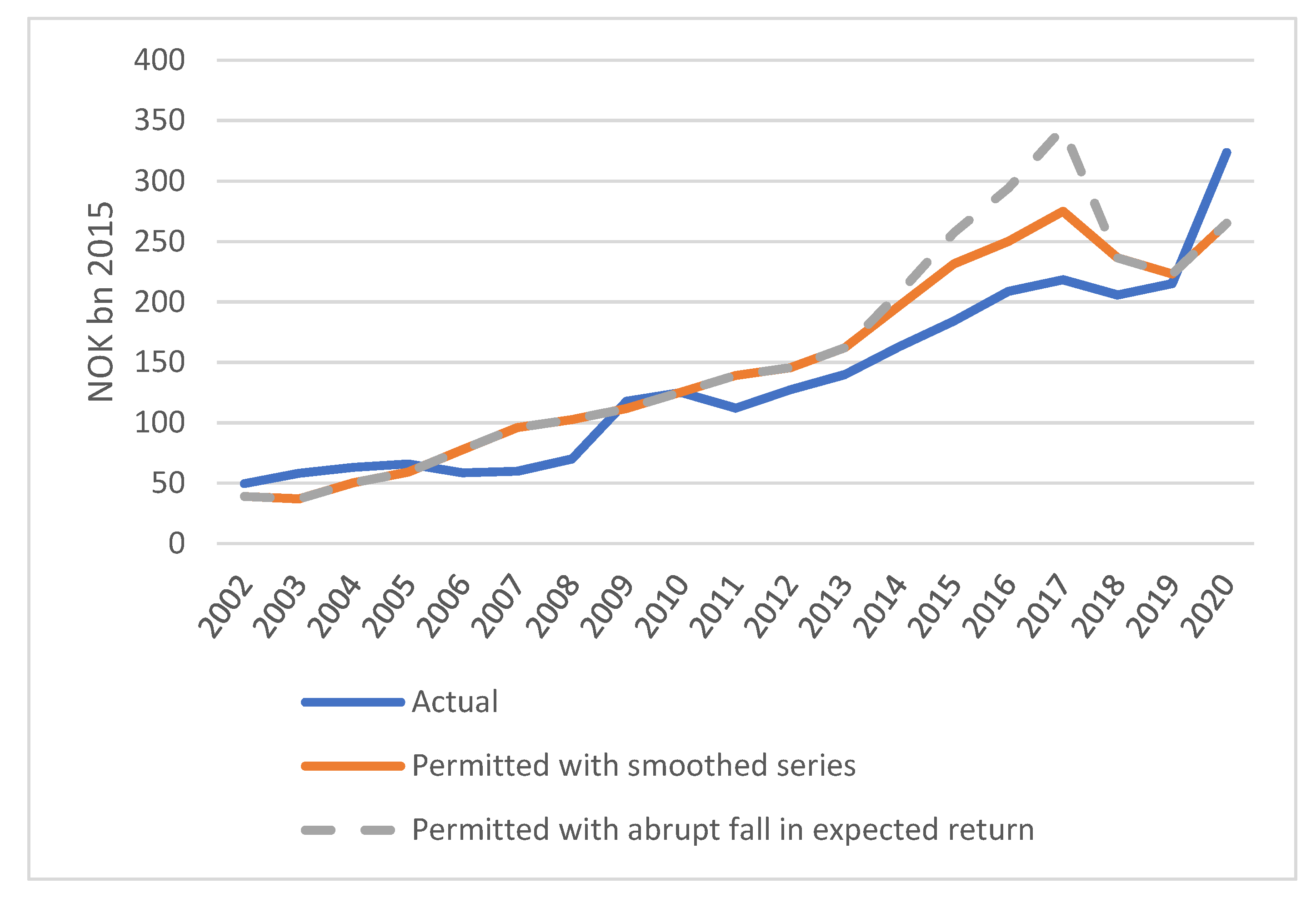
Figure 3 displays the movements in the actual structural deficits and the permitted levels according to our smoothed series as well as the raw series implied by the abrupt drop in $\overline{r}$ from 4 to 3 percent in 2018. The upward trend in all series reflects the persistent growth of the fund as new oil and gas revenues have been deposited. The graph furthermore shows how actual structural deficits increasingly fell short of the upper limit between 2013 and 2018. In fact, they also stayed below our smoothed series. The drop in the smoothed series from 2017 to 2018 is due to the negative real return on the fund that year and is thus not a result of smoothing. The 2020 performance is naturally dominated by the COVID-19 pandemic.

In simulating fund withdrawals, we need the fiscal variables in natural units, i.e., NOK trillions at fixed prices. However, for modeling their time-series behavior, we note that the absolute magnitudes of fiscal actions tend to follow the same trend as real GDP. In Norway’s case, we follow the common practice of using real mainland GDP, i.e., GDP for all sectors except oil and gas extraction9. With this motivation, we specify our time-series model for the fiscal variables in units of percent of trend mainland GDP, with the latter estimated from the same sample as the model, i.e., 1991–2020.

The variables included in our model are thus the real USD-denominated equity return, denoted $r_Q$, the corresponding period return on bond investments, $r_B$, the log real exchange rate, $v_t$, real automatic stabilizers as a percent of trend mainland real GDP, $x_t$, and discretionary fiscal spending (and/or tax cuts), also as a percent of trend mainland GDP, $f_t$.

The movements in the Norwegian business cycle are contained in the residuals of the equations for the two fiscal variables. They thus summarize the combined effects of the various shocks driving this cycle. Because our main contribution lies in the simulation of the possible future movements of the fiscal variables, we find this parsimonious representation of the business cycle preferable to a more comprehensive specification of the underlying shocks and transmission mechanisms behind these movements.

As a preliminary exercise, we use univariate Dickey–Fuller tests to examine the variables’ stationary properties. The results are presented in

Table 1. Dickey–Fuller test results.

Variable	$\widehat{\mathit{\rho }}$	$\left(\widehat{\mathit{\rho }}-1\right)/\mathit{s}.\mathit{e}.\left(\widehat{\mathit{\rho }}\right)$
${\mathit{r}}_{\mathit{Q}}$	−0.0943	−5.7011
${\mathit{r}}_{\mathit{B}}$	−0.0897	−5.8739
$\mathit{v}$	0.6980	−2.2487
$\mathit{x}$	0.7887	−2.2164
$\mathit{f}$	0.8689	−2.0542

Based on OLS equations including constant terms, but no time trends. Variables defined as in the text.

. For the two rates of return, we easily reject unit roots. For the exchange rate, a unit root cannot be rejected on the 10 percent level in our sample. However, as noted in Section 2, we obtain significance on this level when we extend the sample back to the end of the Bretton Woods system in 1971. Stationary is furthermore implied by the hypothesis of long-run purchasing power. Because specifying the exchange rate as stationary also helps us avoid unreasonably high or low exchange rate projections in the simulations, we maintain stationarity as our main hypothesis.

For the detrended fiscal variables, we are unable to reject unit roots on statistical grounds. However, because non-stationarity would be economically unsustainable, we treat them as stationary as well. As in the case of the exchange rate, the stationarity assumption saves our simulations from blowing up because of unreasonably large deviations from the historical experience.

Informal inspection of the data suggests that the Norwegian business cycle is somewhat correlated with the global financial markets. This correlation appears to be especially strong during periods of crisis; however, our sample is too short to allow modeling of time-changing correlations. As a substitute, we look for possible asymmetries by distinguishing between the effects of positive and negative rates of return.

We thus specify a VAR model for our five variables with the modification that the coefficients of lagged rates of return are allowed to be asymmetric. We limit the lag length to two years on a priori grounds. For the equity and bond rates of return, $r_Q$ and $r_B$, respectively, we are unsurprised to find no significant coefficients for their own lags or for those of any other variables.

The exchange rate shows signs of positive dependence on the two-year lags of stock returns. The implication would be that exchange-rate changes are forecastable two years in advance, over and above the eventual return to purchasing-power parity, which we find unreasonable for an asset price. Furthermore, the coefficient that we find is unstable across subsamples. When tested on rolling samples going back to the end of the Bretton Woods system in 1971, with the S&P 500 as a proxy for our equity-return variable, it seems to have arisen mainly during the bull market and subsequent dollar strengthening of the late 1990s and to have faded somewhat during the 2010s. When added to our a priori reasons, this instability convinced us to treat this in-sample correlation as spurious and thus restrict all the lagged variables for the exchange rate to zero, except only for its own lag as implied by stationarity.

For the fiscal variables, we hold no such prior notions. Thus, for the lag coefficients of these equations, we eliminate insignificant coefficients one by one, starting with the ones with the highest p-values, and continuing until all p-values are 0.1 or less. We then use bootstrapping to estimate 90 percent confidence intervals for the contemporaneous correlations of the residuals, constrain to zero those whose intervals contained zeros, and re-estimate the model as a system of seemingly unrelated equations with the resulting residual covariance matrix. The estimation results are presented in

Table 2. Estimation results, annual data 1991–2020.

	${\mathit{r}}_{\mathit{Q}\mathit{t}}$	${\mathit{r}}_{\mathit{B}\mathit{t}}$	${\mathit{v}}_{\mathit{t}}$	${\mathit{x}}_{\mathit{t}}$	${\mathit{f}}_{\mathit{t}}$
Constant	0.0600 (0.0328)	0.0286 (0.0106)	0.8901 (0.2891)		−0.0594 (0.0253)
${\mathit{r}}_{\mathit{Q},\mathit{t}-\mathbf{1}}^{+}$					0.0384 (0.0146)
${\mathit{r}}_{\mathit{Q},\mathit{t}-\mathbf{1}}^{-}$				−0.0309 (0.0060)	−0.0466 (0.0061)
${\mathit{r}}_{\mathit{B},\mathit{t}-\mathbf{1}}^{-}$					0.0962 (0.0267)
${\mathit{r}}_{\mathit{B},\mathit{t}-\mathbf{2}}^{-}$				0.0828 (0.0214)	0.0547 (0.0192)
${\mathit{v}}_{\mathit{t}-\mathbf{1}}$			0.6883 (0.1036)		0.0195 (0.0089)
${\mathit{x}}_{\mathit{t}-\mathbf{1}}$				1.1278 (0.1142)
${\mathit{x}}_{\mathit{t}-\mathbf{2}}$				−0.3716 (0.1172)	0.1528 (0.0705)
${\mathit{f}}_{\mathit{t}-\mathbf{1}}$					0.7760 (0.0471)
SEE	0.1766	0.0570	0.1054	0.0049	0.0045
Residual correlation matrix:
	${\mathit{r}}_{\mathit{Q}}$	${\mathit{r}}_{\mathit{B}}$	$\mathit{v}$	$\mathit{x}$	$\mathit{f}$
${\mathit{r}}_{\mathit{Q}}$	1	0	0	0	0
${\mathit{r}}_{\mathit{B}}$		1	−0.4395	0	0
$\mathit{v}$			1	0.3566	0.4750
$\mathit{x}$				1	0
$\mathit{f}$					1
	${\mathit{r}}_{\mathit{Q}}$	${\mathit{r}}_{\mathit{B}}$	$\mathit{v}$	$\mathit{x}$	$\mathit{f}$

Variables and estimation method defined as in the text. Heteroscedasticity-robust standard errors in parentheses.

.

Here, we note that the automatic stabilizer variable, $x_t$, which most closely (though inversely) parallels the Norwegian business cycle, rises whenever the global stock market declines. We interpret this effect as driven by the international transmission of the global business cycle, with the lag possibly reflecting the fact that the stock market tends to move before the real economy. Such impulses as well as domestic shocks then set off highly persistent movements in the left-hand variable. Perhaps surprisingly, we find no effect on this variable of lagged changes in discretionary fiscal policy, $f_t$, nor are the two significantly correlated contemporaneously.

The discretionary fiscal variable $f_t$ displays a more complex dependence on the lagged values of stock and bond returns. Although the structural meaning of each individual coefficient may not be immediately clear, the main point seems to be a somewhat similar sensitivity to global stock market movements as the automatic stabilizers. Persistence is high for this variable as well. The positive dependence on lagged movements in the automatic stabilizers, $x_t$, can be interpreted simply as fiscal action to stabilize the business cycle.

We note that discretionary fiscal spending tends to increase when the krone declines and vice versa. Because Norway does not have a specific exchange-rate target (at least not after 1999), we believe this coefficient reflects reactions to movements in the price of oil, as an oil price decline tends to weaken the krone while also giving rise to policy measures to counteract the negative effects on the domestic oil sector.

Although the residual variance is lower for the discretionary fiscal variable than for the automatic stabilizers, the total variation in the sample is significantly higher for the former. This difference becomes important in the simulations.

The negative contemporaneous correlation between the real bond return $r_B$ and the real exchange $v_t$ appears to reflect the weakening effect on the dollar of a softening in the global business cycle (recall that high period bond returns tend to reflect falling yields to maturity). The positive contemporaneous correlations between the exchange rate and both fiscal variables seem instead to reflect the likely weakening of the krone in response to weakening of the Norwegian business cycle.

4. Simulation Model

Our simulations are based on the model of the preceding section. For the vector of innovation terms, ${\epsilon }_t={\left({\epsilon }_{Qt},{\epsilon }_{Bt}{\epsilon }_{vt},{\epsilon }_{xt},{\epsilon }_{ft}\right)}^{\prime }$, we assume:

$${\epsilon }_t~\mathcal{N}\left(0,\mathsf{\Sigma }\right),$$

(8)

where the elements of $\mathsf{\Sigma }$ are as estimated in Table 2. From this distribution, we make one million different pseudo-random draws, each for 40-year or 80-year periods. To avoid sampling errors to cause differences between the scenarios, we use the same draws for all the cases we simulate. Spot checks indicate that no significant distortion has been introduced this way.

The normality assumption means that we ignore third and fourth order moments. This means, in particular, that we ignore possible fat tails in the distribution of the financial returns. We do this out of convenience; however, we note that ignoring fat tails tends to bias our results against finding extreme results10. Readers may find our results extreme enough.

Because the fiscal variables in our estimation model are defined as ratios relative to trend mainland GDP, we project future values of the same variables in NOK 2021 trillion by multiplication by the projected future mainland GDP, using the Government’s assumption of 1.4 percent growth per year11 from the actual 2020 trend level. We also consider alternative growth rate assumptions as robustness checks.

Because the Norwegian fiscal rule is based on the fund value in Norwegian kroner, we need to simulate the future development of the fund in the same unit. The annual log real return in real Norwegian kroner becomes, as indicated in Section 2:

$$r_t=\omega r_{Qt}+\left(1-\omega \right)r_{Bt}+v_t-v_{t-1},$$

(9)

where $\omega$ is the equity share, initially fixed at $\omega =0.7$.

The fiscal rule requires the annual withdrawals to equal the expected annual return, which we denote $\overline{r}$, currently officially estimated at 3 percent. We do not necessarily endorse this estimate, which is lower than implied by our estimates in Table 2. However, empirical estimates of first-order moments of financial variables are unlikely to be precise in general, as noted by Maenhout (2004); Pastor and Stambaugh (2012); and Sargent and Stachurski (2021). For this reason, and to analyze the internal consistency of the fiscal rule, we accept the official estimate for the purpose of our simulation exercises.

Letting $r_{Q0}$ and $r_{B0}$ denote the estimated expectations of $r_{Qt}$ and $r_{Bt}$ in Table 2, respectively, we modify the rates of adjustment for equity and bond returns, respectively, while maintaining the estimated equity premium, by choosing the number $z$ such that:

$$\omega \left(r_{Q0}-z\right)+\left(1-\omega \right)\left(r_{B0}-z\right)+\frac{1}{2}{\sigma }_r^2=\ln \left(1+\overline{r}\right),$$

(10)

where ${\sigma }_r^2$ is the variance of $r_t$ implied by the estimated parameters, and $\overline{r}=0.03$. Then, the annual gross return:

$$R_t=e^{r_t}$$

(11)

has the expectation $1+\overline{r}$.

However, implementing this modification in the equations for the two fiscal variables would modify their unconditional expectations as well, leading to simulated variables unreasonably far removed from the historical experience. To avoid that problem, we omit the modification in (10) when simulating the values of the equations for the two fiscal variables.

For a given draw of $r_t$, the fund develops according to:

$$A_{t+1}=\max \left\{A_t{e}^{r_t}-D_t,0\right\},$$

(12)

where the “max” specifies zero as an absorbing barrier. That is, if the withdrawal $D_t$ for any simulated scenario in any particular period $t$ exceeds the fund’s value before the draw is made, we constrain the fund’s value to zero for all subsequent periods in that scenario. This assumption means that we do not consider the possibility of borrowing.

Because our model has lags of up to two years, we assign values to the lagged variables equal to their respective unconditional expectations. For our first actual simulation year, we fix the initial fund value at 12 (2021 NOK trillion), roughly its magnitude at the time the research was done12. We present the simulated future fund values as percentages of this value.

4.1. Fiscal Rule Implementation

The specification of the withdrawal $D_t$ is key to our analysis. Because, in the Norwegian case, the law requires all non-oil government deficits to be drawn from the fund (as long as there is money in the fund), each annual draw equals the sum of the structural non-oil deficit and the automatic stabilizers:

$$D_t=S_t+X_t.$$

(13)

As explained in the preceding section, the structural, non-oil deficit can be separated into the structural, non-oil deficit permitted under the fiscal rule and discretionary fiscal spending that may make the actual structural, non-oil deficit deviate from that rule:

$$S_t={\overline{S}}_t+F_t.$$

(14)

Thus, the annal withdrawal can be decomposed into three parts:

$$D_t={\overline{S}}_t+F_t+X_t.$$

(15)

In the simulations, we compute ${\overline{S}}_t$ as $\overline{r}{A}_t.$ The draws of the model residuals, the definition of $r_t$, and the lag coefficients then yield values for $x_t$ and $f_t$, which in turn are multiplied by the projected future mainland GDP to obtain values for $X_t$ and $F_t$, respectively.

4.2. Specification of Smoothing

Fund owners typically prefer smooth withdrawals to choppy ones. Fiscal rules such as the Norwegian one aim to facilitate such smoothness by allowing withdrawals to be made according to expected rather than actual returns. Even so, the fiscal rule can produce large, abrupt changes in the structural, non-oil deficit in cases of substantial changes in the fund’s value. Similarly large changes could result if discretionary fiscal spending in one year is cut to zero the following year so as to bring the structural, non-oil deficit back to its stipulated value ${\overline{S}}_t$.

Such abruptness can be mitigated by one or both of the fiscal variables. However, the Norwegian fiscal rule allows for even more flexibility by permitting—indeed mandating—explicit smoothing of the structural, non-oil deficit13. We model this smoothing as a partial adjustment:

$$S_t=\lambda S_{t-1}+\left(1-\lambda \right){\overline{S}}_t+F_t, 0\le \lambda \le 1.$$

(16)

The last term in Equation (16) implies that discretionary fiscal spending in period $t$ comes on top of the structural, non-oil deficit implied by the smoothing rule. We consider this formulation realistic because we believe that decisions on this item will be made based on stabilization needs as perceived in period $t$ and are thus not part of a return to normal. The continuation of stimulation measures into 2022 because of the advent of the Omicron strain of COVID-19 illustrates this point. However, this formulation also means that the discretionary fiscal spending in our simulations may differ from the definition implicit in Equation (7), which we have applied to construct the data for $F_t$ used in our estimations. This difference is logically consistent if we also assume that smoothing was not practiced during our sample period. We return to this question in the next section.

It is worth noting that smoothing of the structural, non-oil deficit does not translate directly into smoothing of the actual withdrawals. The difference is made up by the automatic stabilizers in addition to new fiscal spending. Thus, the actual withdrawals with smoothing become:

$$D_t=\lambda D_{t-1}+\left(1-\lambda \right){\overline{S}}_t+X_t-\lambda X_{t-1}+F_t$$

(17)

5. Simulation Results

We simulate our model 40 years into the future, starting from a fund value of 12 (NOK trillions 2021).

Table 3. Simulation results, main scenarios. Distribution of fund value 40 years hence. Fund sizes are stated as percentages of the starting value. No explicit smoothing.

	No Fiscal Policy a	Automatic Stabilizers Only b	Full Fiscal Policy c
5%	14.5%	10.8%	3.5%
25%	31.9%	29.3%	26.0%
50% (median)	55.2%	53.4%	51.4%
75%	95.6%	94.7%	93.1%
95%	211.0%	212.1%	209.1%
Mean	76.9%	75.3%	72.4%
Depletion rate	0.0%	0.3%	3.5%

^a. The variables $X$ and $F$ are both constrained to zero. ^b. The values of $X$ are simulated as described in the text, whereas the values of $F$ are constrained to zero. ^c. Both $X$ and $F$ are simulated as described in the text.

displays the quantiles of the fund value after 40 years as well as its mean value, in percent of the starting value, and the percentage of scenarios where the fund is depleted by the end of the 40-year period. As a simplest first case, we constrain both fiscal variables to zero throughout the simulation period. Then, we add the automatic stabilizers and lastly also the discretionary fiscal policy. No further smoothing is added at this stage.

The first point to note in these results is the median fund value, which is little more than half of its current level. This is the very uncomfortable implication of the theorem by Dybvig and Qin (op. cit.) discussed in Section 2. The claim, often made by Norwegian policy makers, that adherence to the fiscal rule is “responsible” in the sense that it preserves the fund for future generations, simply does not hold water.

We secondly note that the mean fund value after 40 years is barely larger than three-quarters of its starting value. This difference reflects the result, also discussed in Section 2, that the negative serial correlation of financial returns induced by the long-term stationarity of the real exchange rate implies an expected future fund value that is lower than its current value even though the draws are restricted to equal the expected return. We are surprised to see the magnitude of this effect. Because we believe the stationarity assumption to be realistic, we feel this result raises a flag that has previously not been raised in the policy debate nor in the literature.

As a test of robustness, we estimated an alternative model where we required the exchange rate to follow a random walk. As expected, the mean fund value then equaled the starting value when no fiscal variables are included and only trivially lower with full fiscal policy. Interestingly, however, the median values were remarkably similar. The rest of the distributions are similar as well except for the 95 percent quantiles, which are larger with the random-walk specification, as expected. We thus venture to conclude that our results have not been distorted by the stationarity assumption for the exchange rate.

Although the distribution is heavily skewed to the right, we find no cases of actual depletion when both fiscal variables are constrained to zero. It remains minor also when the automatic stabilizers are added. However, discretionary fiscal policy raises the risk noticeably. The 3.5 percent chance of depleting the fund within 40 years may not be large, yet it seems more than high enough to raise some concern.

The effects of the fiscal variables clearly depend on the amplitude of the Norwegian business cycle. In our model, we assume that it rises over time at the same rate as the trend growth of mainland GDP.

Table 4. Simulation results with varying trend growth rates.

	Trend Growth Rate 0.7%		Trend Growth Rate 1.4%		Trend Growth Rate 2.1%
	40 Years	80 Years	40 Years	80 Years	40 Years	80 Years
5%	6.1%	0.0%	3.5%	0.0%	0.0%	0.0%
25%	27.1%	0.1%	26.0%	0.0%	24.6%	0.0%
50% (median)	51.9%	23.3%	51.4%	19.9%	50.9%	10.0%
75%	93.3%	59.9%	93.1%	60.6%	93.1%	62.5%
95%	209.1%	192.9%	209.1%	194.3%	209.2%	200.2%
Mean	73.1%	51.0%	72.4%	49.6%	71.7%	48.6%
Depletion rate	2.2%	25.0%	3.5%	35.1%	5.3%	45.9%

Distribution of fund value 40 and 80 years hence. Fund sizes are stated as percentages of the starting value. No explicit smoothing. Full fiscal policy in all cases.

presents the sensitivity to varying growth assumptions, where we look at cases with half or double the government’s official forecast of 1.4 percent. The case without fiscal policy is unaffected by this assumption, so we limit the presentation here to the realistic case of full fiscal policy. Paradoxically, the depletion risk rises with the growth rate. The reason is that when higher growth makes the economy larger in the later years, the fiscal demands on the fund during recessions become greater. With withdrawals equal to the expected return, on average, the fund will not, as a central tendency, grow with the economy, thus tending to make the fiscal strains on the fund more severe over time.

Because this effect grows over time, we find it useful to include the same cases simulated over 80 rather than 40 years. We then see how the mean and median shrink as the time horizon grows, as predicted by the theory in Section 2. After 80 years, the depletion risk becomes a substantial 46 percent.

The business-cycle amplitude can also change independently of the trend growth rate. Our model has been estimated on data from a period where the dominating industries in Norway were oil and gas extraction, with important additions of oil supply and service14. The cyclical movements of these industries have at times deviated from those of neighboring and other developed economies. Because fiscal policy typically aims to stabilize business cycles, Norwegian fiscal policy may behave differently from our estimated model once the country’s petroleum era comes to an end. Predictions of how this difference may look will necessarily be speculative, however, as long as we do not know the industry structure of the Norwegian post-oil economy.

What does seem clear is that the Norwegian business cycle has been significantly smoother over the last 30 years than that of neighboring Sweden and Denmark, as expressed, for example, by the GDP gaps estimated by the IMF. Based on the differences between these estimates, we add a simulation case where the residual standard deviations of the fiscal variables both are increased by 85 percent, while keeping the trend growth rate at 1.4 percent. The results for the 40-year horizon, including full fiscal policy, are displayed in

Table 5. Simulation results, wider business cycle fluctuations.

	Estimated Business Cycles	Wider Business Cycles
5%	3.5%	0.0%
25%	26.0%	25.6%
50% (median)	51.4%	52.8%
75%	93.1%	96.0%
95%	209.1%	214.0%
Mean	72.4%	73.7%
Depletion rate	3.5%	5.7%

Distribution of fund value 40 years hence. Fund sizes are stated as percentages of the starting value. No explicit smoothing. Full fiscal policy in all cases. Wider business cycles: Residual standard deviation in equations for X and F raised 85%. Trend growth rate: 1.4%. No explicit smoothing.

along with the original results in Table 3. Although the higher variability of fiscal policy increases the variability of the future fund value, the differences are much more modest than the ones in Table 4. The reason is that the wider business-cycle fluctuations now hit earlier, when the fund is larger in most scenarios. The fund size then acts as a cushion against greater losses.

Neither means nor medians change much. The slight increases in the median may perhaps be explained by the fact that the presence of the fiscal variables introduces an element of normality in a distribution that is otherwise lognormal, as noted in Section 2. However, the risk of depletion does increase from 3.5 percent to 5.7 percent. Although the results in Table 5 do not identify changes in the business cycle as a major risk, the higher risk of depletion may serve as an admonition for policy makers to watch for changes in the business cycle when oil and gas cease to be part of the picture.

6. Smoothing

As mentioned in Section 4.2, the fiscal rule itself implies a kind of smoothing in that draws are calibrated to the expected financial return, i.e., as a constant percentage of the fund value, rather than the highly variable percentages implied by the realized returns. The fiscal variables add further smoothing to the extent that the fund value is positively correlated with the domestic business cycle. Even so, the text of the Norwegian fiscal rule allows a third layer of smoothing to avoid large, abrupt changes in the structural, non-oil deficit. We specified a formula for such smoothing in Equation (16).

For that equation to be consistent with the rest of our model, we need to assume that smoothing has not influenced the data behind our estimated model in any important way. If it did, the observed non-oil, structural deficits would already have been smoothed, so that adding another layer of smoothing would make the model internally inconsistent.

One might hope to resolve this question empirically by estimating the value of the smoothing parameter $\lambda$ implied by the available data. An estimate close to zero would then imply little or no smoothing in the data, so that adding the smoothing feature in Equation (16) would allow simulation of future fund performance if behavior is changed from no smoothing to smoothing.

An estimation equation would have $\left(S_t-{\overline{S}}_t\right)\equiv F_t$ on the left and $\left(S_t-{\overline{S}}_{t-1}\right)$ on the right (or both variables divided by trend mainland GDP). However, by definition, the error term would then be identical to the left-hand variable and thus correlated with the right-hand variable if $\lambda >0$. Furthermore, even if this problem is ignored, we find the estimate of $\lambda$ to depend crucially on a few outliers in the sample. If they are ignored, the estimate would be close to unity; if they are included, it would be essentially zero.

Less technically, we would argue that the rapid growth of the fund’s value during our sample period has made smoothing superfluous even on occasions when it has been intended. The political process behind the 2010 budget may serve as an illustration of this point. When presented to the Storting in October of 2009, the government’s budget proposal implied a structural, non-oil deficit corresponding to 5.7 percent of the expected fund balance as of January 2010, significantly higher than the 4 percent that was then the norm15. The government projected this deficit to stay constant in real kroner for another seven years. The fund was not expected to grow enough for this deficit to be consistent with the fiscal rule until 2017. As things turned out, the economy recovered faster than expected, resulting in a 5 percent lower structural, non-oil deficit for 2010. The fund also grew much faster than expected, partly because of higher-than-expected oil and gas revenues, partly because of favorable exchange-rate movements, and partly because of a strong stock-market recovery after the global financial crisis. As a result, the structural, non-oil deficit stayed within the 4 percent norm already in 2010.

We interpret this episode as suggesting that our data are consistent with no significant realized smoothing, but that the political willingness to smooth nevertheless is strong enough to justify simulations with the smoothing in (16) added.

That leaves the question of an appropriate numerical value for the smoothing parameter $\lambda$. In the absence of reliable estimates, we treat $\lambda =0.5$ a reasonable guess, implying that half of a gap would be closed the first year. However, we also consider $\lambda =0.8$ as an alternative case. This much slower smoothing, where only one fifth of a gap is closed the first year, may serve as an approximate description of the decision making in the fall of 2010. It is furthermore consistent with the so-called MIT-Tobin rule, which reportedly is practiced by a number of U.S. university endowment funds16.

Table 6. Simulation results with and without smoothing.

	$\mathbf{No} \mathbf{Smoothing} (\mathit{\lambda } = 0)$		$\mathbf{Smoothing} (\mathit{\lambda } = 0.5)$		$\mathbf{Smoothing} (\mathit{\lambda } = 0.8)$
	No Fiscal Policy	Full Fiscal Policy	No Fiscal Policy	Full Fiscal Policy	No Fiscal Policy	Full Fiscal Policy
5%	14.5%	3.5%	13.4%	0.0%	9.7%	0.0%
25%	31.9%	26.0%	30.3%	19.1%	25.5%	0.0%
50% (median)	55.2%	51.4%	53.5%	47.6%	48.6%	35.2%
75%	95.6%	93.1%	94.2%	91.6%	91.1%	92.9%
95%	211.0%	209.1%	213.0%	211.1%	220.2%	234.2%
Mean	76.9%	72.4%	76.1%	69.0%	73.8%	65.1%
Depletion rate	0.0%	3.5%	0.0%	10.9%	0.0%	31.4%

Distribution of fund value 40 years hence. Fund sizes are stated as percentages of the starting value. Trend growth rate: 1.4%.

presents the implications of smoothing along with the results without smoothing, repeated from Table 3. In all cases, smoothing shifts the distribution to the left. The effects are distinctively stronger in the presence of full fiscal policy. A higher than 10 percent probability of depletion within 40 years if one-half of all gaps are closed within one year ($\lambda =0.5$) should cause some alarm. We consider this degree of smoothing fairly realistic for government use of sovereign wealth funds. The slower adjustment where only one-fifth is closed the first year ($\lambda =0.8$) may be more realistic for other endowment funds. However, for such funds, the nearly one-third probability of depletion may be less relevant because such funds are not responsible for countercyclical fiscal policy.

The contrast with the effects of smoothing in the absence of fiscal policy, which are also included in Table 6, suggests that smoothing of the effects of large changes in fund value present much less of a risk of fiscal sustainability than the smoothing back to normal after periods of extraordinary large fiscal spending. Interestingly, not even smoothing with $\lambda =0.8$ raises the depletion probability above zero if the government refrains completely from fiscal policy. Although we have not studied limits on fiscal policy, this finding suggests that such limits should be able to reduce the depletion risk even in the presence of smoothing.

Dybvig and Qin (op. cit.) raise the issue of so-called death spirals in the presence of smoothing. For example, after a large drop in fund value, smoothing would imply subsequent withdrawals at a higher percentage than the expected return. Such positive feedback could perhaps deplete the fund quickly. Dybvig and Qin conclude that such death spirals can indeed occur and propose limits on the smoothing process to avoid them. As an analysis of possible death spirals in our model, we consider a case where a substantial equity loss occurs in the second year of all simulated scenarios after establishing the common starting point in the first year, while keeping the real exchange rate unchanged between the first and the second year. The subsequent development could then be called a death spiral if all subsequent scenarios lead to depletion.

Table 7. Simulation of development with smoothing after initial equity shock.

	$\mathit{\lambda }=0.5$			$\mathit{\lambda }=0.8$
Shock size	10%	50%	90%	10%	50%	90%
5%	0.0%	0.0%	0.0%	0.0%	0.0%	0.0%
25%	16.3%	0.0%	0.0%	0.0%	0.0%	0.0%
50% (median)	43.0%	15.1%	0.0%	30.9%	0.0%	0.0%
75%	83.2%	40.8%	0.0%	85.7%	18.5%	0.0%
95%	190.8%	101.1%	0.0%	215.8%	102.4%	0.0%
Mean	62.1%	28.1%	0.0%	59.3%	18.8%	0.0%
Depletion rate	12.3%	33.8%	100.0%	33.5%	68.4%	100.0%

Distribution of fund value 40 years hence. Fund sizes are stated as percentages of the starting value. Full fiscal policy. Trend growth rate: 1.4%.

presents the results in the presence of full fiscal policy.

The results demonstrate, first of all, that large losses leave long shadows. That follows from the fact that withdrawals are calibrated to match the expected return on average, so that the fund will not be automatically replenished after a loss. In this sense, all losses are permanent (as are all gains). Second, the risk of depletion is high in all cases17. However, for losses as low as 10 percent, comparison with the fourth and sixth column in Table 6 suggests that the depletion risk is driven more by the smoothing than by the initial loss. Death spirals do occur in the sense of a 100 percent depletion risk. However, that only happens if the initial loss is extremely large, such as 90 percent. For losses limited to 50 percent, the depletion rate is limited to two thirds even with the very slow smoothing of $\lambda =0.8$. We thus dare conclude that the risk of true death spirals is very low. We also want to add that after an event that is dramatic enough to cause such a large, global stock-market decline, other concerns are likely to take priority over the preservation of the fund. That said, the risk of large losses should probably not be taken lightly.

7. Remedies

Despite the many challenges facing sovereign wealth funds and endowment funds, some of which have been studied in the preceding sections, they are not doomed to depletion. Good management can reduce the risk of depletion and even avoid it completely. Naturally, any such measure will carry costs. Whether or not the gains justify the costs will be a matter of investor preferences, which we do not specify in this paper.

One such step would be to take down risk by reducing the portfolio’s equity share. That would smooth out movements in the fund’s value and hence in withdrawals without explicit smoothing.

Table 8. Comparison of simulation results with 50–50 vs 70–30 portfolio.

No Smoothing	70% Equity		50% Equity
	No Fiscal Policy	Full Fiscal Policy	No Fiscal Policy	Full Fiscal Policy
5%	14.5%	3.5%	23.9%	13.0%
25%	31.9%	26.0%	42.9%	36.7%
50% (median)	55.2%	51.4%	64.3%	60.5%
75%	95.6%	93.1%	96.5%	94.2%
95%	211.0%	209.1%	173.5%	172.0%
Mean	76.9%	72.4%	77.2%	72.5%
Depletion rate	0.0%	3.5%	0.0%	1.0%
$\mathbf{Smoothing}, \mathit{\lambda }=0.5$	70% Equity		50% Equity
	No Fiscal Policy	Full Fiscal Policy	No Fiscal Policy	Full Fiscal Policy
5%	13.4%	0.0%	23.0%	0.0%
25%	30.3%	19.1%	41.9%	29.8%
50% (median)	53.5%	47.6%	63.4%	57.0%
75%	94.2%	91.6%	95.9%	93.6%
95%	213.0%	211.1%	174.4%	174.9%
Mean	76.1%	69.0%	76.6%	68.9%
Depletion rate	0.0%	10.9%	0.0%	5.6%

Distribution of fund value 40 years hence. Fund sizes are stated as percentages of the starting value. Trend growth rate: 1.4%.

shows the results of reducing the equity share from 70 percent to 50 percent in our model portfolio. The upper panel compares the results of 70 percent and 50 percent equity without smoothing, whereas the lower panel gives the same comparison with smoothing imposed with $\lambda =0.5$. Although the depletion risk is modest even with the 70–30 portfolio, especially without smoothing, we note that it is even lower with a less risky one. Furthermore, the medians are much higher and the expected values almost identical. The reason is that the lower volatility of the portfolio returns delays the concentration of probability mass near zero discussed in Section 2. It does not eliminate it, however.

The obvious cost of this strategy is that withdrawals are reduced with the expected portfolio return from 3 percent to 2 percent. Even this effect is cushioned somewhat by the fact that the fund’s value tends to be more safely preserved over time. However, lowering the equity share does not solve the fundamental problem of the almost sure eventual depletion if withdrawals are calibrated to the expected portfolio return.

To overcome this problem, the size of withdrawals must be lower than the expected return. The question is how much. In the absence of fiscal policy and smoothing, Section 2 gives the answer as one-half the variance of the instantaneous portfolio return in Norwegian kroner, which with our data works out as 1.4 percent, so that the maximum sustainable withdrawal rate would be 1.6 percent. With fiscal policy and smoothing, which we consider the realistic case in practice, the issue becomes trickier because the distribution of future fund sizes is no longer quite lognormal.

As a practical approach, we look instead for the withdrawal rate that would leave the median value of our fund equal to its starting value after 40 years with full fiscal policy and smoothing with $\lambda =0.5$. The result is 1.3 percent, just a little lower than in the absence of fiscal policy. The simulation results are displayed in

Table 9. Comparison of simulation results with withdrawal rates lower than vs equal to the expected rate of portfolio return.

40 Years Hence	$\mathbf{No} \mathbf{Smoothing} (\mathit{\lambda }=0)$		$\mathbf{Smoothing} (\mathit{\lambda }=0.5)$
	3% Withdrawal	1.3% Withdrawal	3% Withdrawal	1.3% Withdrawal
5%	3.5%	18.1%	0.0%	5.5%
25%	26.0%	56.3%	19.1%	50.1%
50% (median)	51.4%	103.5%	47.6%	100.0%
75%	93.1%	182.4%	91.6%	181.4%
95%	209.1%	402.4%	211.1%	405.1%
Mean	72.4%	143.8%	69.0%	140.4%
Depletion rate	3.5%	0.9%	10.9%	3.8%
80 Years Hence	$\mathbf{No} \mathbf{Smoothing} (\mathit{\lambda }=0)$		$\mathbf{Smoothing} (\mathit{\lambda }=0.5)$
	3% Withdrawal	1.3% Withdrawal	3% Withdrawal	1.3% Withdrawal
5%	0.0%	0.0%	0.0%	0.0%
25%	0.0%	33.8%	0.0%	6.2%
50% (median)	19.9%	100.5%	0.0%	88.2%
75%	60.6%	235.8%	57.7%	227.7%
95%	194.3%	738.5%	199.3%	736.7%
Mean	49.6%	204.3%	46.2%	194.6%
Depletion rate	35.1%	12.3%	51.0%	23.7%

Distribution of fund value 40 years hence. Fund sizes are stated as percentages of the starting value. Full fiscal policy. Trend growth rate: 1.4%.

. The upper panel shows the results after 40 years, with and without smoothing. The results with 3 percent withdrawals are also shown for comparison. The median value is indeed preserved with smoothing. Without smoothing, the median value is even higher, but only by 3.5 percent, suggesting that smoothing is not the big issue so far. Although the depletion risk has not been eliminated, it has been reduced significantly.

40 years may seem like a long horizon. However, a search for sustainability should look even further. The lower panel in Table 9 looks at the results after 80 years. In the absence of smoothing, the median still looks pretty good, with a preservation of 100.5 percent of the starting value. However, smoothing reduces this figure to 88.2 percent. Moreover, the depletion risk is now substantial. Even without smoothing, cutting the withdrawal rate from 3 percent to 1.3 percent results in depletion withing 80 years in about one-eighth of all cases.

The culprit is clearly fiscal policy. Now, our model specifies the fiscal policy variables as normally distributed. That means, among other things, that no limit is put on fiscal stimulus in times of recession. Our data sample is too small to test the realism of this assumption. However, because sustainability can be secured if fiscal policy is forsaken altogether, effective limits on fiscal deficits should go a long way towards the same goal. Many states, such as the United States and the EU member states, have imposed such limits, though with mixed success. Because the purpose of this paper is to provide policy analysis rather than policy advice, we leave this issue to policy makers’ political judgment.

A common argument in the debate about the Norwegian fiscal rule is that 3 percent is a conservative estimate of the expected real return. Indeed, as we noted in Section 4, reliable estimates of expected financial returns are hard to come by. However, if we accept the argument, we may want to ask what the true expected rate of return would have to be to make the 3 percent rule for withdrawals sustainable. We sought an answer to that question along the same lines as the exercise underlying Table 9. The answer is 4.8 percent, or 1.6 percentage points higher than 3 percent. We do not want to pass any judgement of the realism of expecting 4.8 percent real return on a 70–30 global portfolio. However, we do believe that many observers would put this estimate in the high range of their estimation intervals.

Would there not be warning signs along a path towards depletion? There probably would. If the fund loses much of its value over, say, the first 20 years, a correction could be implemented in the form of limits on fiscal spending, including regular withdrawals, until the fund has rebuilt itself. We suspect that such a strategy would be less efficient than setting a sustainable course from the beginning; however, to make such a judgement, we would again have to make assumptions about investor preferences.

8. Conclusions

Long-term investors face a number of challenges. Among the most important is the tradeoff between withdrawals to finance current spending needs and the preservation of the fund for future generations. The rule often used of allowing draws corresponding to the expected financial return is intuitively appealing. A board of supervision, a parliament, or voters at large may find it convenient to use as a disciplinary tool or as a yardstick to judge the soundness of spending decisions or proposals. In the context of the Norwegian Government Pension Fund Global, it is the essence of the fiscal rule. Its main appeal is that it can be claimed to preserve the mathematical expectation of the fund’s future value, seen from the present, at a level equal to the current fund value. It does not, however, guarantee the fund’s long-term survival even if strictly adhered to. In fact, it leads almost surely to the fund’s eventual depletion. This is not a hypothesis; it is a mathematical theorem.

Further complications are likely to pile up on top of this one. Small-country investors who diversify their assets in global markets, but make withdrawals for local use, face an additional risk factor from exchange-rate movements, which typically imply negative serial correlation for returns in the local currency. With such correlation, the fiscal rule does not even preserve the expected future value of the fund but biases it towards zero.

In practice, decision makers want flexibility to deviate from the rule. A seemingly innocent deviation is to allow countercyclical variations to ensure smooth funding of the services that the fund withdrawals are supposed to fund. In the Norwegian context, this flexibility is codified by applying the fiscal rule to the structural rather than the actual budget deficit, so that the automatic fiscal stabilizers are allowed to work freely. In practice, draws on a sovereign wealth fund will also be used to fund discretionary fiscal policy. The effects of such deviations from the main rule may not only be large. They also change the shape of the probability distribution of future fund values. Because policy innovations are likely to be more or less normally distributed, their inclusion transforms the distribution of future fund values from lognormal to a hybrid of lognormal and truncated normal with a spike at zero. As a result, depletion becomes a real risk over horizons of 40 years or shorter. Explicit smoothing on top of this flexibility, which is often favored by policy makers and codified in the Norwegian case, add to this risk.

The mean and median problems can be remedied by requiring withdrawals at substantially lower rates than the expected rate of portfolio return. The increase in depletion risks caused by fiscal policy can furthermore be reduced by choosing less risky assets, e.g., by lowering the equity share. However, eliminating depletion risks further requires bounds on fiscal policy.

Further advice on what to do would require some kind of specification of investor preferences regarding the various tradeoffs involved. A particularly sticky point is how to specify the desire for smoothness and discretionary fiscal policy. Although the preservation of fund value for future generations have been codified in the GPFG Act, this objective has not been accompanied by limitations of fiscal actions beyond the rather vague stipulation in the fiscal rule that excessive draws in times of need be followed by subsequent fiscal tightening. In a companion paper (Mork et al. 2022), we explore a possible specification of this tradeoff.

The experience of the Norwegian Government Pension Fund Global so far has been benign with steady growth in the fund’s value and no occasions where draws from the fund had to be curtailed, not even after the global financial crisis. However, this 20-year period has been unusual in that sizeable deposits from the government’s oil and gas revenues have been made every year. Real tests of smoothness and sustainability are much more likely to come once these revenues start to dry up.